Revisiting the multidecadal variability of North Atlantic Ocean circulation and climate

1 Introduction

The World Ocean and almost all its regions have been warming since the late 1960s, with a robust temperature rise in upper ocean heat content during that time, e.g (Kuhlbrodt et al., 2007; Levitus et al., 2012; Johnson and Lyman, 2020; Cheng et al., 2022). This indisputable fact implies that ocean currents also change in response to ongoing surface warming, e.g (Thorpe et al., 2001; Hu et al., 2004; Toggweiler and Russell, 2008; Johnson and Lyman, 2020). However, there is still no consensus about the strength or extent of these changes, especially in those assessed by climate models, e.g (Chen et al., 2019; Couldrey et al., 2023). Moreover, whether these changes are persistent and can be extrapolated into the foreseeable future or are at all predictable is still being determined. To meet this challenge, many eyes have been on the North Atlantic (NA)—one of the most potent drivers of the global ocean circulation and a great contributor to the Earth’s climate variability. Such an immense role of the NA is upheld by the most powerful ocean current system of the Northern Hemisphere—the Gulf Stream and its extensions comprising the upper arm of the Atlantic Meridional Overturning Circulation (AMOC), e.g (Kuhlbrodt et al., 2007; Saba et al., 2016; Bower et al., 2019; Zhang et al., 2019; Jackson et al., 2022); see comprehensive reviews of the NA research over decades and the AMOC functionality in (Lozier, 2012; Yashayaev et al., 2015; Buckley and Marshall, 2016; Frajka-Williams et al., 2019; Johnson et al., 2019; Jackson et al., 2022). There are clear indications that two intermingling processes comprise the recent decadal NA climate trajectory — a slow warming trend and multidecadal variability superimposed on that slow trend (Seidov et al., 2017). The conversion of warm and salty ocean waters transported to deep convection sites in high latitudes is responsible for the operation of the AMOC (Bower et al., 2019). Therefore, understanding the upper ocean’s circulation changes amid ongoing surface warming brings us closer to better grasping the overall ocean climate variability of the NA climate caused by upper-ocean warming. We approach the multidecadal variability of the NA ocean climate change and related variability of the AMOC by expanding our previous work reported in (Seidov et al., 2017) by adding salinity and density analyses to the sole temperature analysis. We also add a thermohaline circulation evaluation to illustrate thermohaline variability. Our main working hypothesis is that seawater temperature and salinity, and therefore density from long-term observations, can serve as fingerprints of the ocean circulation, including the AMOC changes over half a centennial time frame.

Many ocean parameters varying in time may be fingerprints of the ocean circulation and overall ocean climate change, e.g (Jackson and Wood, 2020). For example, sea surface temperature can be a fingerprint of the ocean circulation, e.g (Latif et al., 2004). The results of ocean models can be used to produce a fingerprint, for example, sea surface temperature emerging in a climate simulation model, e.g (Caesar et al., 2018), or combining sea surface elevations with subsurface hydrological observations, e.g (Zhang, 2008), or any combination of multiple observed or modeled ocean variables, e.g (Msadek et al., 2010; Mahajan et al., 2011; Zhu et al., 2023). According to (Jackson and Wood, 2020), a useful AMOC fingerprint should represent an aspect of the AMOC to monitor. The relationships between the variables selected as fingerprints and the AMOC should be understood physically, and these variables must be observable. The in-situ temperature, salinity, and density data covering the NA on a multidecadal time scale ideally satisfy those criteria because the ocean thermohaline circulation and, therefore, AMOC as one of its elements, are closely related. The circulation forms the thermohaline structure through heat and freshwater fluxes across the sea surface and wind stress, and in turn is shaped by the thermohaline structure via sea surface elevation and density gradients (Sarkisyan and Sündermann, 2009) (Gill, 1982; Pedlosky, 1996; Marshall and Plumb, 2007). Many authors have tried to predict the changes in the AMOC using selected fingerprints, e.g (Msadek et al., 2010; Mahajan et al., 2011), and most recently (Ditlevsen and Ditlevsen, 2023), who predict the collapse of the AMOC by the mid of 21^st century. The goal of this study is to not predict future AMOC changes, but instead to diagnose the changes in temperature, salinity, and density as fingerprints of the NA circulation variability. Through this diagnosis we can try to assess the changes in the upper limb of this circulation to evaluate possible AMOC alterations over several decades.

The surface NA circulation is a complex pattern of warm and cold currents. A schematic view of the NA currents system, based on the general knowledge of ocean currents in the North Atlantic, e.g (Schmitz and McCartney, 1993; Rossby, 1999; Richardson, 2001; Reverdin et al., 2003), is shown in Figure 1. As Figure 1 implies, the major elements of the NA surface circulation are two large gyres—the anticyclonic subtropical gyre of warm and saline water and the cyclonic subpolar gyre of colder and somewhat fresher water. The warm subtropical surface waters move poleward, cool down, lose buoyancy, sink, and return southward in deeper layers, typically below one-kilometer depth. The Gulf Stream and its extensions—the North Atlantic Current and, further to the east, the North Atlantic Drift, comprise the warm poleward flow of the AMOC upper limb. After downwelling in the deepwater formation sites in the deep ocean, return flow, which forms the deep limb of the AMOC, completes the overturning loop in the NA. The AMOC has been intensely investigated in various studies, and a few review papers analyze and summarize those efforts, e.g (Lozier, 2012; Buckley and Marshall, 2016; Weijer et al., 2019; Zhang et al., 2019; Caínzos et al., 2022; Johnson et al., 2022).

Figure 1

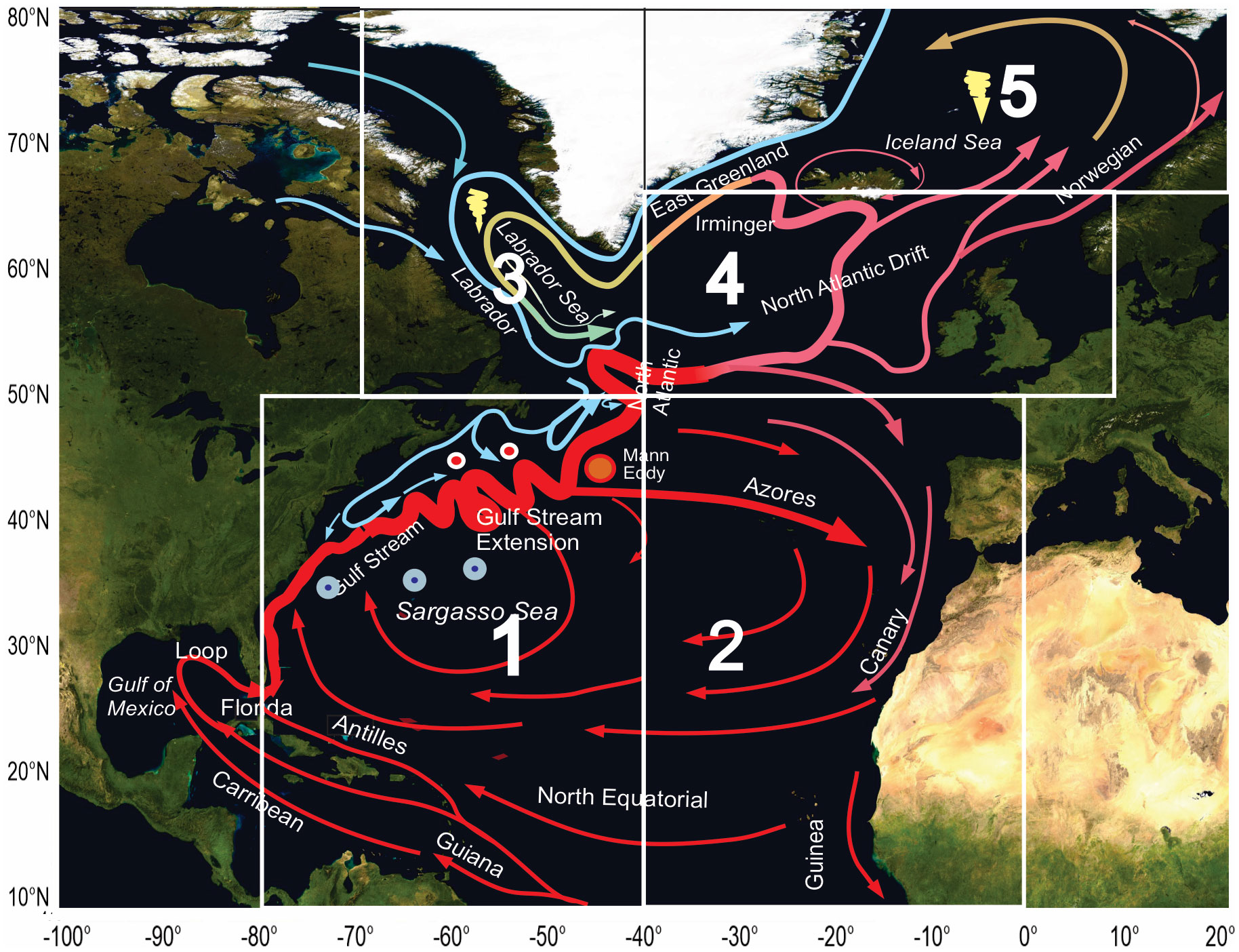
Figure 1 A scheme of the upper-layer circulation of the North Atlantic Ocean. Red – warm currents, blue – cold currents. White boxes 1 to 5 indicate five different areas of analysis where temperature, salinity, and current velocities presumably differ considerably. Comparative analysis of the averages of various variables in the entire NA and each box can shed additional light on how the NA climate system functions and help better understand how stable this system is as a whole and in its segments.

There are consensuses and differences in opinion on the AMOC’s dynamics and long-term variability. The uncertainties regarding the AMOC’s current state, recent changes, and its fate in the near and more distant future stem from the enormous complexity and strong variability on various time spans, from seasonal to multiyear, to centennial, and longer. In fact, the true 3-D version of the NA circulation on those time intervals with multiple interplaying factors, such as mesoscale eddies, ocean-atmosphere interactions, etc., is only attainable in eddy-resolving ocean circulation models, even better in coupled high-resolution climate models. A multitude of such modeling efforts addresses specifically the AMOC dynamics and variability, e.g (Cheng et al., 2013; Drijfhout, 2015; Zhu et al., 2015; Mecking et al., 2016; Sévellec and Fedorov, 2016; Chen et al., 2019; Megann et al., 2021; Lin et al., 2023), and many others. The Arctic Seas changes can also impact the AMOC functionality, e.g (Liu et al., 2019; Liu and Fedorov, 2022). Moreover, the feedbacks between the AMOC and the Arctic’s sea ice loss can be one of important feedbacks affecting the overall AMOC dynamics and thus NA ocean climate trajectory, i.e., the weekend AMOC can diminish recent sea ice loss (Liu et al., 2017; Lee and Liu, 2023).

The cited and other modeling efforts revealed many aspects of the AMOC functionality. They tried to hindcast and forecast AMOC’s variability and sensitivity to external sources, including the changes in atmospheric CO₂, sea surface salinity changes, changes in freshwater exchange across the sea surface, etc. The results of the very first model of the global ocean circulation response to freshwater fluxes across the sea surface were reported in (Manabe and Stouffer, 1988), showing that there could be two stable equilibria in a coupled ocean-atmosphere model. Since then, there have been many research efforts using the modeling approach to reveal the global meridional circulation and, in particular, the AMOC response to the impacts of freshwater release into the ocean in the NA high latitudes, either by specifying variable or constant freshwater fluxes or employing the so-called “hosing” numerical experiments, with low salinity patches applied at seas surface, e.g (Rahmstorf, 1994; Manabe and Stouffer, 1995; Rahmstorf, 1995; Seidov et al., 2005; Stouffer et al., 2007).

According to the IPCC, 2021 report, there is a wide range of uncertainty regarding the strength and timing of the AMOC, stemming from the models and reanalyses, ranging from subtle changes to nearly complete collapse by the end of the 21st century (IPCC, 2021). The observations present a highly variable view of the current and future states of the AMOC. However, unlike the models, they suffer from uneven data distribution in both space and time. The analyses of such direct observations of some proxies vary significantly in their assessments of the AMOC changes over short and long periods of time. Most often cited direct measurements of the AMOC intensity were reported in (Bryden et al., 2005). Since then, many observations, in sync with some of the above-cited (Ditlevsen and Ditlevsen, 2023) model experiments, indicated that the AMOC began to slow down during the last two decades, presumably due to the continued warming of the ocean surface and, possibly, to the accompanying changes in the salinity of the upper layers of the ocean (Srokosz et al., 2012; Smeed et al., 2018; Rhein et al., 2019; Lin et al., 2023). However, the magnitude of these changes is still under dispute, e.g (Jackson et al., 2022).

While the recent AMOC slowdown is hard to deny, the suggestion that the NA circulation has changed dramatically or at least very significantly requires further examination, and the messages about the possible collapse of the AMOC, e.g (Behrens et al., 2013; Drijfhout, 2015), cannot be ignored. Moreover, a number of the NA-specific features, such as the NA warming hole (or cold blob), can most easily be explained by the AMOC weakening (Rahmstorf et al., 2015), albeit the complexity of this phenomenon calls for full three-dimensional analysis that would combine eddy-resolving modeling, direct observations, and reanalyzes studies. Liu and co-authors (Liu et al., 2020) also provide compelling arguments that the AMOC slowdown is the cause of the North Atlantic warming hole. The key to understanding the AMOC dynamics is having a better insight into how the upper limb of the AMOC operates, especially in its origin—the Gulf Stream and its extensions.

A recent study has shown that the Gulf Stream, the central part of the upper arm of the AMOC, has been remarkably resilient over the last five decades (Seidov et al., 2019b). Moreover, the warming of the North Atlantic Ocean is uneven in space and time (Zika et al., 2021). The most significant accumulation of heat is, at least partially, associated with the sinking of the subtropical mode water or eighteen-degree water (EDW) at the southeastern flank of the Gulf Stream, e.g (McCartney and Talley, 1982; Talley and Raymer, 1982; Bindoff and McDougall, 1994; Hanawa and Talley, 2001; Huang, 2015; Häkkinen et al., 2016; Seidov et al., 2019a; b). Substantial transformation of the ocean circulation would supposedly be attested to a structural altering of density gradients, a function of both temperature and salinity. Therefore, these changes should be seen in decadal climatologies, such as those in the latest edition of the World Ocean Atlas published in 2018, which we refer to as WOA18 (Boyer et al., 2018). Although decadal variability is present in WOA18, it cannot be easily seen in temperature, salinity, and density maps. Even in the most recent high-resolution ocean climatologies of the Northwestern Atlantic region (Seidov et al., 2022), which can be perceived as “eddy-resolving” in-situ climatologies (Seidov et al., 2019a), the decadal variability is noticeable but not excessive. Therefore, the climate shift in the NA can be better assessed and visualized as anomalies, i.e., by comparing two climates (Seidov et al., 2017) or as deviations from an averaged state of several decades.

Thus, we consider the changes in multiple essential ocean variables—temperature, salinity, density, and current velocities over 60+ years. We analyze the decadal variability of the entire NA and its sub-regions and refer to each decadal average as a “decadal ocean climate” or simply “ocean climate.” Decadal climates are then referenced to the “climate normal,” which defines the Earth System climate (see more details in the following section).

To address this predicament, we employed the global decadal climatic fields of temperature, salinity, and density from the WOA18 (Boyer et al., 2018) and extracted the values for the NA domain comprised by the boxes 1 to 5 in Figure 1 (data are available at WOA18). These climatologies cover six decades from 1955–1964 to 2005–2017 (the last “decade” contains 13 years of data instead of ten as in all other decades, but for convenience, we refer to it as a decade nonetheless). We also used climate reanalysis data on decadal wind stress and sea surface height (SSH) fields from the Simple Ocean Data Assimilation project (SODA version 3.4.2, http://www.soda.umd.edu) (Carton et al., 2018). Since the SSH data from SODA were unavailable before 1980, these data were used only for the last three decades—1985-1994, 1995-2004, and 2005-2017. Despite this reanalysis record being shorter than some other reanalysis products, we use the same SODA data for consistency with our previous analysis in (Seidov et al., 2017; Seidov et al., 2019a).

2 Research strategy and methods

The research strategy can be broadly perceived as three significant steps to disentangle the critical factors controlling the NA climate change in response to long-term surface warming. By focusing on the thermohaline circulation variability on decadal time scales, we isolate the thermohaline components and concentrate on its decadal change amid ongoing surface warming. Therefore, the first step is to explore the wind field’s variability. The decisive wind field characteristic for large-scale ocean circulation is the wind stress curl (WSC) rather than the wind stress (Gill, 1982). The WSC is responsible for the geometry and intensity of the wind-driven ocean circulation. In the crudest approximation, the two most essential elements of the North Atlantic currents system - the subtropical and subpolar gyres - correspond to the negative (anticyclonic) and positive (cyclonic) WSC over the sea surface, respectively.

The WSC over the entire NA is shown in Figure 2A where a straight line indicates the approximate position of the zero WCS value. The position on zero WCS is very stable over time, which is illustrated by Hofmuller diagrams in Figure 2B – the small north-south drift of the zero WCS position (60°W, 40°W, and 20°W) is evident and plotted at three different longitudes over the 1980-2019 period. The differences in WSC between the two decades of 2005-2017 and 1985-1994 are shown in Figure 2C. The WSC defines the upward or downward Ekman pumping areas—the upward or downward vertical velocities at the base of the Ekman mixed layer. The downward pumping occurs in regions with negative WSC, and the upward pumping (or suction) in areas with positive WSC. These compensating vertical water motions are due to the diversion or conversion within the Ekman’s layer caused by the wind stress-induced flows. The downward Ekman pumping occurs mainly within the subtropical (anticyclonic) gyre, while the upward pumping takes place within the subpolar (cyclonic) gyre (see Figure 1 for schematic reference). The two gyres are separated (approximately) by the line of WSC=0 (Figure 2A). The differences in WSC in Figure 2C delineate where the pumping, upward or downward, has increased or decreased over 30 a 30-year period from 1985 to 2017.

Figure 2

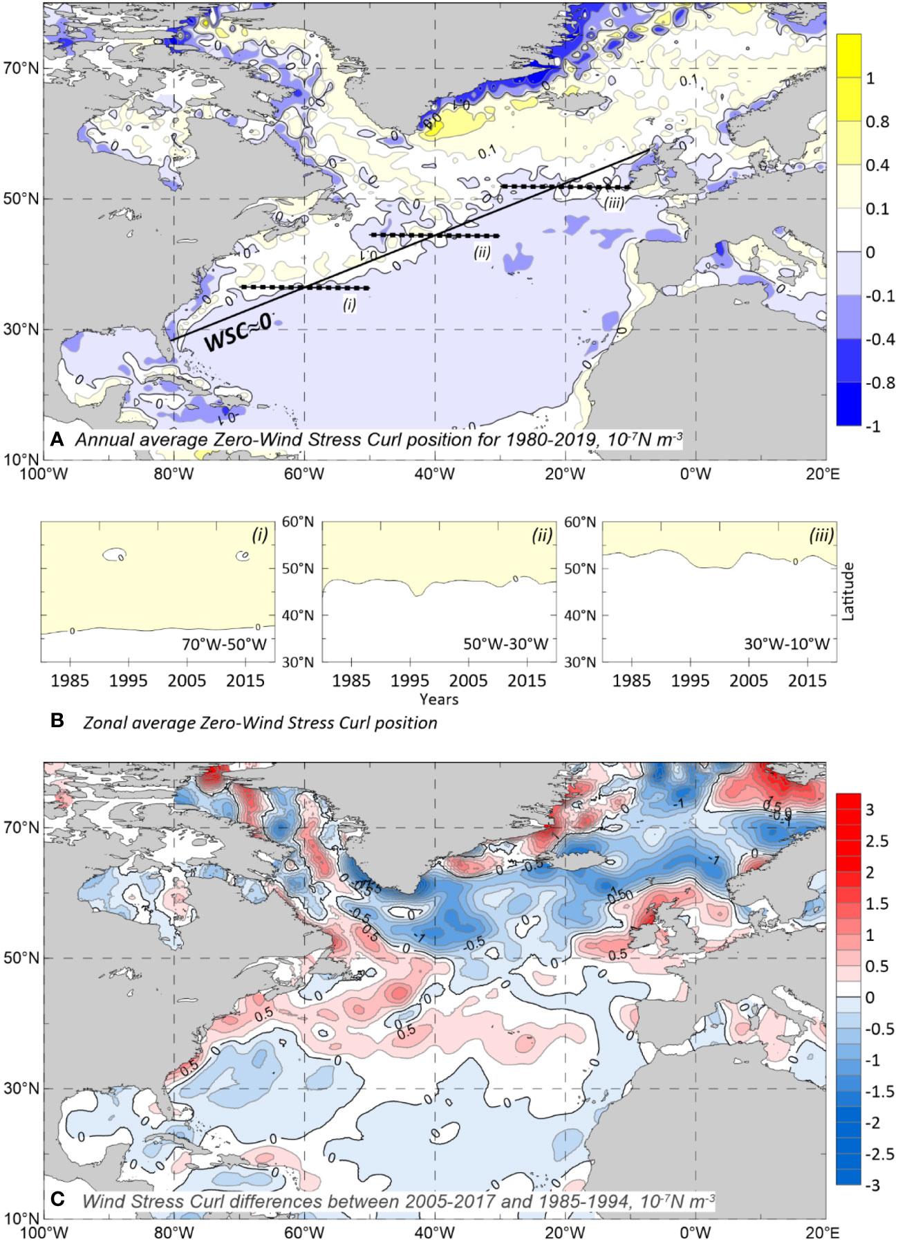
Figure 2 The average annual wind stress curl (WSC) over 1980-2017 (A), and changes in the zonal averages for three sections of zero line of the WSC position (B). A straight line approximates the zero WSC position; the zonal averages of the WSC≈0 position is shown by dotted consecutive lines in (A). WSC differences between 2005-2017 and 1985-1994 (C). The WSC and its differences are in 10^-7 N·m^-3.

The sign and magnitude of the WSC determine the main NA ocean gyres. Digging deeper, the position of the zero line of WSC controls the change in the size and shape of the aforementioned gyres. Using SODA data, we calculated the average WSC over the 1980-2017 period (Figure 2A) and the change in the zonal averages for three sections of the zero WSC line position (Figure 2B). The zero WSC position is approximated by a straight line in Figure 2A; the intervals over which the zonal averages of the WSC≈0 positions were computed are shown by dotted consecutive lines in Figure 2A. The large-scale features of the WSC are like those in (Chelton et al., 2004) and dissect the NA diagonally from Florida to the British Isles.

As seen from Figure 2B, there is practically no long-term trend in the average position of the zero line of the WSC at different longitudes. This outcome supports our assumption that the geometry of the circulation gyres produced by the wind changed very little over a long period. Thus, we can ignore the wind component variability if we focus on ocean circulation changes driven by surface thermohaline transformations.

Ignoring the wind-induced velocities (i.e., Ekman transport) does not mean that the influence of the wind is absent in our analysis. We do not imply that wind stress is not essential for the thermohaline circulation. Quite the opposite, the WSC is paramount for structuring the thermohaline ocean circulation via Ekman pumping and westward intensification of the density fields. Without the wind stress forming and maintaining the major ocean gyres, the AMOC would have been completely shut down (Timmermann and Goosse, 2004). Here, we argue that the decadal variability of the WSC and its most critical element—the position of its zero line—has not changed substantially. Thus, we can focus exclusively on the long-term variability of the thermohaline circulation. However, although Ekman drift velocity is not directly included in our calculations, Figure 2C is critically important for understanding and interpreting the thermohaline circulation changes. The WSC plays a crucial role in the formation and sustaining of the ocean-wide circulation gyres and in local impacts of Ekman pumping on heaving or upwelling warm or cold water. Therefore, Ekman pumping is responsible for creating local density gradients driving thermohaline currents.

Moreover, our previous work found that the WSC is critically important for the local accumulation of the ocean heat (Seidov et al., 2019a). The changes in the intensity and location of Ekman pumping are essential for local distribution and redistribution of ocean heat content, as Figure 2C suggests. However, despite some oscillatory behavior, the overall position of the zero line of the WSC did not change over the last 60+ years, and therefore the geometry of the wind-induced ocean gyres remained stable, which justifies our decision to exclude the Ekman velocities and transport from analysis of the decadal-scale circulation changes.

The second step of our study is to assess temperature, salinity, and density decadal variations relative to defined climate normals for these variables in the entire NA and the selected five regions. The World Meteorological Organization defines the climate normals using 30-year periods, routinely called “climate normals” (WMO, 2018). According to this definition, the Earth’s climate and, therefore, the climate of the upper ocean layers is approximated by a thirty-year average of any climate-forming parameters in the ocean. For this study, these are temperature, salinity, and density. For further analysis of the NA within the geographical limits shown in Figure 1, we define the reference climate or “climate normal” as the average fields of temperature, salinity, and density over the three “middle” decades, i.e., the period of 1965-1994, with all decadal climatologies referenced to these climate normals to produce decadal anomalies. Using earlier and cooler decades for computing the climate normal allows us to emphasize the rapid changes that occurred during the most recent decades of 1995-2017. It should be noted that if we used a different climate normal, the anomalies would have changed, but the change in anomalies between each decade would remain relatively constant, and therefore choosing a different climate normal would not matter.

The third step contains the calculation of the current velocities for analyzing the decadal changes of the ocean circulation caused by the upper ocean warming. As was mentioned above, the geometry of WSC did not change significantly, and substantial changes in the upper arm of the AMOC can mostly be due to the significant alteration of current velocities induced by seawater density gradients. Therefore, we calculate only the geostrophic component of the horizontal velocity vector. The equations for computing the horizontal components of the geostrophic velocity are:

$\begin{array}{ll}v=\frac{1}{{\rho }_{0 }f}\frac{\partial p}{\partial x}& (1)\end{array}$

$\begin{array}{ll}u=-\frac{1}{{\rho }_{0}f}\frac{\partial p}{\partial y}& (2)\end{array}$

$\begin{array}{ll} \frac{\partial p}{\partial z}=g\rho & (3)\end{array}$

where u and v are the west and north-directed components of the velocity vector, respectively; p is the pressure; ρ is the density of seawater: $\rho ={\rho }_0+{\rho }^{\prime }$; ${\rho }_0=1028$kg·m^-3; $f=2\text{Ω}sin\phi$ is the Coriolis force, where Ω is the Earth’s angular rotation speed; Ω = 7.5 10^-5s^-1 and φ is latitude; g is the Earth’s gravitational acceleration g=9.8ms^-1. In the numerical approximation of Equations (1) and (2) on a regular spherical grid $\delta x=\delta ycos\phi$; for a quarter-degree grid, the grid step along a meridian is δy=0.25°(2π/180°)R, i.e., δy≈ 27.8 km, where R is the Earth’s radius; R= 6378 km; depth z is counted downward from the undisturbed sea surface where z=0.

The pressure at any depth z can be computed using Equation (3):

$\begin{array}{ll}{p}_z=p_0+{\rho }_{0}gz+{\rho }_{0}g{\displaystyle {\int }_0^z}\rho \text{'}dz;& (4)\end{array}$

where p_z is the pressure at depth z, and p₀ is the pressure at the undisturbed sea surface level, i.e., at z=0; if the SSH is denoted as ζ relative to z=0, then $p_0={\rho }_{0}g\zeta$ (Sarkisyan and Sündermann, 2009). For the practical purposes, the second term in the right side of Equation (4) can be ignored because it does not contribute to the horizontal gradients of p in Equations (1) and (2), i.e., to use $p_z^{\text{'}}=p_z-{\rho }_{0}gz$, instead of $p_z$, instead of p_z in those two equations. Thus, the only two variables needed for computing the geostrophic currents are the SSH, i.e., ζ (positive upward) relative to z=0 and the density of seawater [more details can be found, e.g., in (Sarkisyan, 1977; Gill, 1982; Sarkisyan and Sündermann, 2009)].

The water density fields are extracted from the WOA18. For the SSH or the elevation of the sea surface relative to the sea surface level z=0, there are two options for its determination. The first and simplest way is to use the so-called dynamic method for calculating velocities relative to a certain “zero-velocity surface” or depth of “no-motion” z=D, where the pressure gradients vanish, e.g (Fomin, 1964; Sarkisyan and Sündermann, 2009). This approach to obtaining surface pressure is the same as in calculating the ocean dynamic topography relative to the no-motion level, here chosen to reside at 1500 m; for more information on the dynamic topography calculations and the dynamic method in oceanography see, e.g (Fomin, 1964; Church et al., 2001; Sarkisyan and Sündermann, 2009). This surface, computed relative to a chosen depth of no-motion, D, gives the value of p₀ in Equation (4), with the second term in the right side dropped:

$\begin{array}{ll}{p}_0={\rho }_{0}g{\zeta }^D;& (5)\end{array}$

where ${\zeta }^D=-\frac{1}{{\rho }_0}{\displaystyle {\int }_0^D}\rho \text{'}dz; D\text{=const, }$here D=1500 m.

The second and more advanced way to calculate sea level pressure at z = 0 is to use the SSH values from the SODA reanalysis data, where p₀ in Equation (5) s the pressure at an undisturbed sea level z=0, where ζ^T is the observed SSH from the SODA reanalysis. Due to the obvious constraints, such data have been available only for the last three decades, but the advantage is that no assumptions about a zero-motion surface in the deep ocean are required. In Equations (1) and (2), the pressure at the surface is either computed using the dynamic method ζ^D using Equation (5) or calculated using ζ^T, which is the SSH values extracted from the SODA dataset (see above).

The level of no-motion used in the dynamic method calculations does not mean there is no flow below z=D. Quite the opposite, the very nature of thermohaline overturning circulation presumes that the equator-to-poles flow of warm and salty water in the upper layers is compensated by a pole-to-equator return flow of cold and fresh water in deeper layers, e.g (Schmitz, 1995). The two flows comprise the thermohaline meridional overturning. The dynamic method assumes a return flow below the no-motion level. Although the method of computing velocities using observed sea surface elevation does not require a no-motion level, the main feature of thermohaline overturning remains intact, and there must be return flows from high to low latitudes.

The intensity of the ocean circulation can be estimated by analyzing the distribution of the specific kinetic energy (kinetic energy per volume of water; in the gridded field—per volume of a grid cell):

$\begin{array}{ll}KE=\frac{1}{2}{\rho }_0\left(u^2+v^2\right) & (6)\end{array}$

where KE is the specific kinetic energy of the geostrophic ocean currents calculated at any depth using Equations (1), (2), and (4). For convenience, in Equation (6) we refer to this specific kinetic energy simply as kinetic energy.

Finally, in addition to the three major steps outlined above, we computed the changes in the decadal northward and eastward oceanic water transport using the geostrophic currents in the upper 1500 m. The formulas for calculating the water transport across a latitudinal or meridional section are:

$\begin{array}{ll}{Q}_M={\displaystyle {\int }_0^D{\int }_{M_1}^{M_2}}vdxdz;& (7)\end{array}$

$\begin{array}{ll}{Q}_L={\displaystyle {\int }_0^D{\int }_{L_1}^{L_2}}udydz;& (8)\end{array}$

where Q_M and Q_L are the northward/eastward meridional/latitudinal water transports, respectively; in Equations (7) and (8) M₁ and M₂ are the western and eastern limits of a latitudinal section, and L₁ and L₂ are the southern and northern limits of a meridional section.

The current velocities play a supplemental and largely diagnostic role because either method of calculating the current velocities are somewhat flawed—the D velocities are far from what would be considered qualitative because of the “no-motion” level assumption that has no analogy in real ocean, while the T velocities, albeit more defendable, are still not what would be considered as a true diagnostic as, for example, in ocean diagnostic models, e.g (Holland and Hirschman, 1972; Sarkisyan, 1977; Mellor et al., 1982; Greatbatch et al., 1991; Sarkisyan and Sündermann, 2009). However, if the main concern is the changes in the circulation of the upper one thousand meters, i.e., the relative numbers, both methods can be used, although the D velocities can be calculated only where the ocean is deeper than 1,500 m. Given this disclaimer, our priorities focus on the thermohaline changes based on the data from WOA18. These changes reflect the circulation changes. The computed current velocities play a supportive role in illustrating those changes better.

3 Results and analysis

We excluded wind stress as a contributor to decadal changes in NA ocean circulation for our study on AMOC’s thermohaline component. Thus, we focused on temperature and salinity decadal variability and the changes in velocity generated by the variations in the density field (and in the alternative approach by the SSH variability). Using the SODA SSH implicitly includes both thermohaline and wind stress variability; it’s important to remember that the observed thermohaline fields from WOA18 already include the wind impact induced by Ekman pumping and advection via gradient and wind-induced currents.

The NA surface is getting noticeably warmer and saltier over the last 60 years (Table 1). Table 1 shows temperature and salinity for the entire NA and Box 1 (Gulf Stream system) for six decades at 50-m depth. The NA near-surface tendencies of both temperature and salinity in the Gulf Stream system (Box 1) and the entire NA are coherent (differences of thermal and salinity regimes in different boxed are discussed in more details further in the text).

Table 1

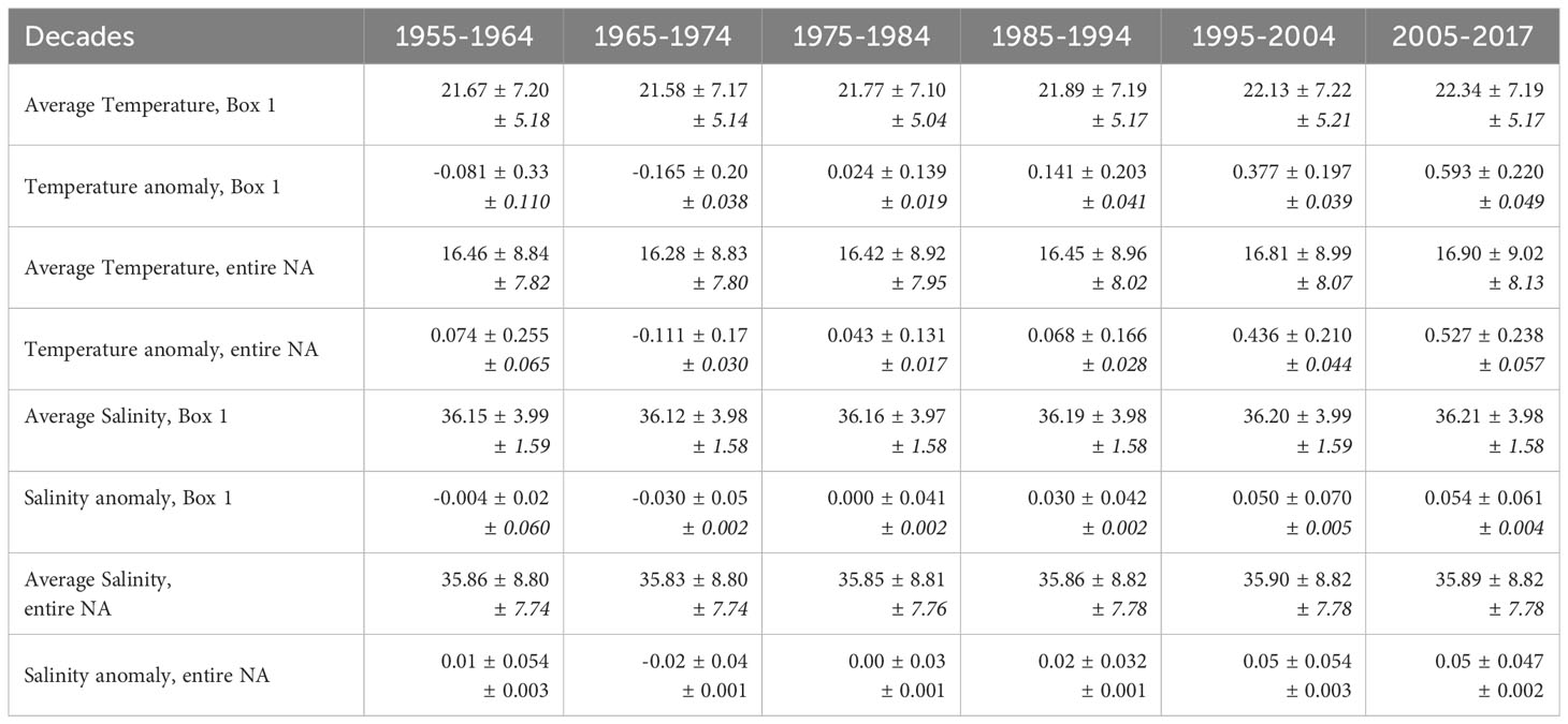
Table 1 Average decadal annual temperature (°C) and salinity and anomalies (vs 1965-1994 climate normals) taken from each 0.25-degree latitude-longitude cell over the Box 1 and the entire NA domain (80°W-20°E; 10°N-80°N) at 50-m depths along with decadal standard deviation (upper numbers) and yearly variance (lower numbers).

As an example, Figure 3 shows the annual climate normal field (1965-1994 average) in the NA and deviations from this normal for the 2005-2017 decade (i.e., values from 2005-2017 minus the 1965-1994 normal). Despite undeniable warming, salinization, and reduction in density of the upper-ocean layer, the deviations of the NA climate are not excessive. The largest deviations in temperature, found in the Gulf Stream region and in the Nordic Seas, are less than 1.5°C and salinity deviations, largely linked to temperature changes, are less than 0.3. The NA surface warms almost everywhere with corresponding density decreases (i.e., the water in the upper layer became warmer, saltier, and lighter). The question then becomes whether such changes lead to substantial variation in the circulation pattern, and whether the deeper layers followed the upper layer tendencies. Moreover, it is important to reveal climate changes in the sub-regions of the NA, and how severe and desynchronized those changes can be. The following analysis aims to show whether the NA ocean climate system has been resilient or fragile to the various changes it has experienced.

Figure 3

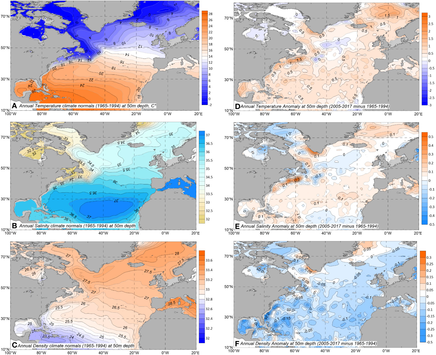
Figure 3 Annual climate normals fields (1965-1994 averages) in the North Atlantic at 50m depth: (A) temperature, °C; (B) salinity; (C) density as σ_t=ρ-1000 (kg·m^-3). Deviations from the climate normals: (D) temperature (°C); (E) salinity; (F) density (σ_t=ρ-1000; g·cm^-3) for the decade 2005-2017 minus 1965-1994 normals.

To reduce the volume of temperature, salinity, density, and velocity arrays to analyze, we looked at only the upper 1500 m of the ocean and only at four depths—z=50, 200, 500, and 1000 m. As all profiles below 200 m vary quasi-linearly with depth, the velocity at the selected levels can well represent the averaged velocity within the layers enclosing those levels. By limiting the maximal depth of data analysis to 1000 m, we focus on verifying whether the AMOC is either slowing down or speeding up within its upper arm, which is critical for the overall diagnostics of the AMOC dynamics. Figure 3 shows our ocean climate normals (decadal averages over 1965-1994) for temperature (A), salinity (B), and density (C), and the anomalies of these variables in the decade of 2005-2017 relative to the climate normals (D, E, and F) at 50 m depth.

Figure 4 depicts the velocity vectors at 50 m depth for the decade of 1995-2004. The D-velocity (Figure 4A) is the velocity calculated using the dynamic method relative to the level of no-motion at D=1500 m, where D stands for dynamic method. Figure 4B shows the T-velocity, where the T stands for the “true” velocity obtained using the SSH from the SODA reanalysis. Both D and T calculations use the density from WOA18.

Figure 4

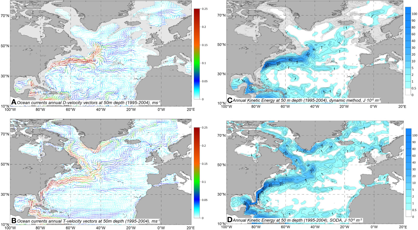
Figure 4 Ocean currents annual velocity vectors (ms^-1) and kinetic energy (J·10^-6m^-3) at 50 m depth for the decade of 1995-2004 calculated by different methods: (A) velocities calculated using the dynamic method relative to 1500 m reference depth; (B) velocities computed using SSH from SODA project; (C) kinetic energy calculated using the velocities obtained using the dynamic method; (D) kinetic energy calculated using the velocities obtained using the seas surface heights from the SODA project. The areas where the ocean is shallower than 1500 m are shown in (A, C) in light gray. Note that the D-velocity was calculated only for areas of the NA deeper than 1500 m; thus, the shelf’s shallow areas and the part of the slope shallower than that reference depth were excluded.

The T-velocity, in contrast, was calculated everywhere, including the shelf area deeper than 50 m. Hence different isobaths are shown in Figures 4C, D. Although noticeable differences exist, there is also a surprising similarity between the two velocity sets where they can be compared (i.e., everywhere the ocean is deeper than 1500 m). Figures 4C, D show kinetic energy at 50 m for the decade 1995-2004 calculated using the D-velocities (Figure 4A) and T-velocities (Figure 4B), respectively. Table 2 shows that, overall, the NA upper-layer circulation intensified from 1955-1964 to 1995-2004 (as revealed in the D-velocities) and then slowed down in the last decade of 2005-2017; SODA gives similar acceleration in 1985-2004 and then slowdowns in the last decade (as revealed in the T-velocity calculations).

Table 2

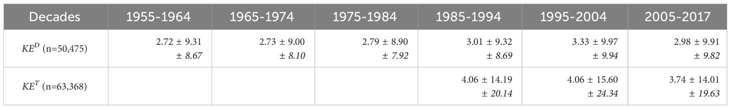
Table 2 Kinetic energy (J·10^-6m^-3) at z=50 m taken from each 0.25-degree latitude-longitude cell averaged over the entire NA domain for six decades computed using D- and T-velocities with standard deviation (upper numbers) and yearly variance (lower number); n shows how many points (cell numbers) were used for calculation of KE (fewer number for dynamic method).

To visualize the decadal variability in the NA (overall and in the five selected regions numbered 1 to 5 as shown in Figure 1), the average annual temperature, salinity, and density deviations from the established climate normal (1965-1994 period) are displayed as bar charts in Figure 5. The figure depicts averaged annual temperature values at 50 m, 200, 500, and 1000 m depth, while Figures 6 and 7 show salinity and density deviations, respectively.

Figure 5

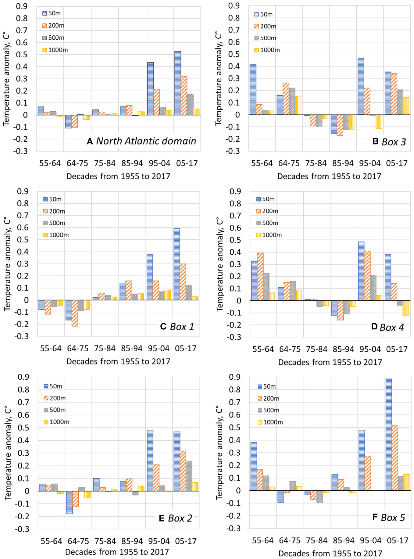
Figure 5 Decadal variability of the annual sea water temperature anomalies at the different depth relative to the climate normals (°C), i.e., the individual decades minus 1965-1994 climate normals: (A) in the entire North Atlantic; (B–F) in the selected boxes 1 through 5 shown in Figure 1. Vertical axis – temperature anomalies, °C; horizontal axis – decades.

Figure 6

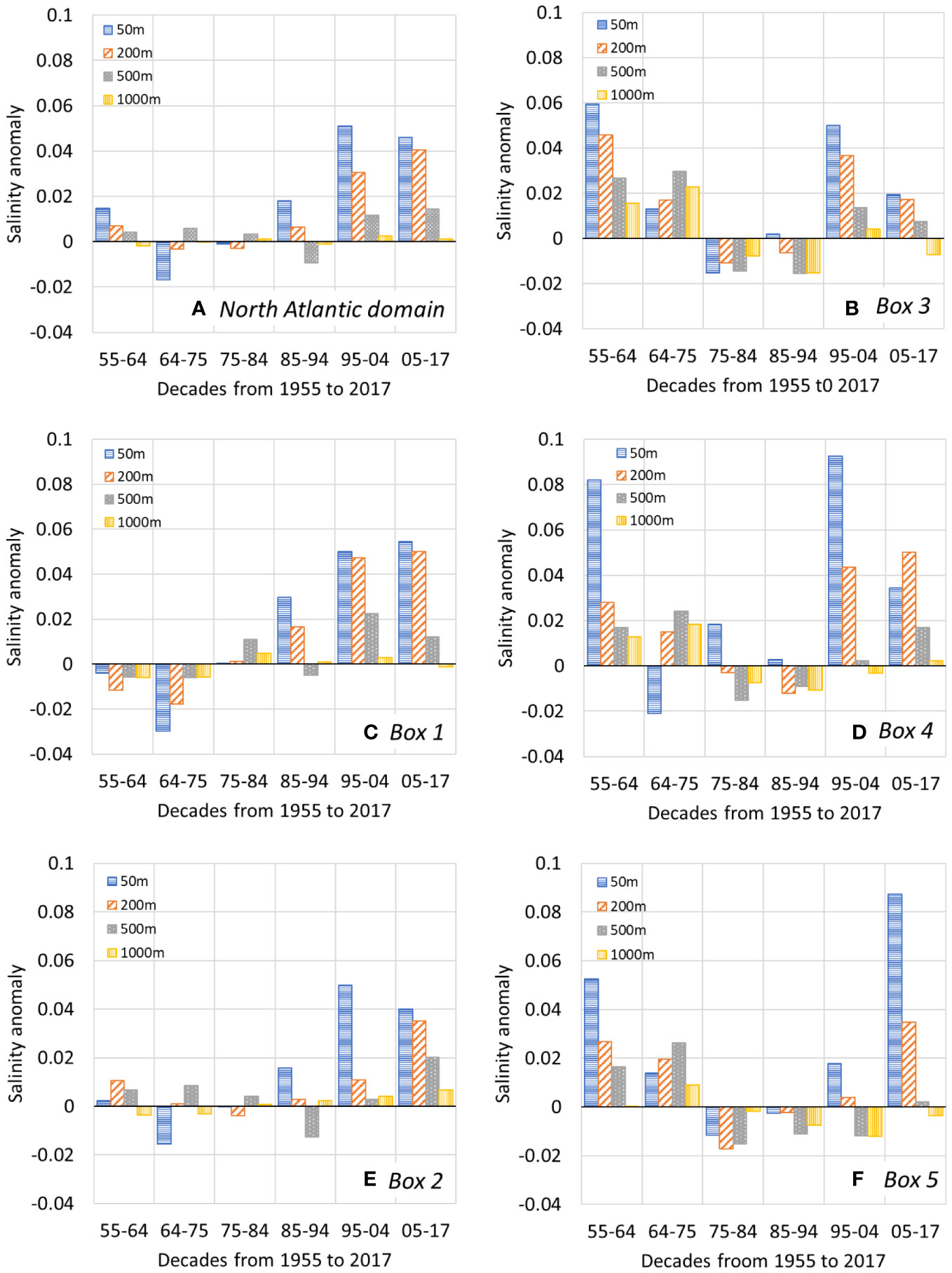
Figure 6 Decadal variability of the annual salinity anomalies at the different depth relative to the climate normals, i.e., the individual decades minus 1965–1994 climate normals: (A) in the entire North Atlantic; (B–F) in the selected boxes 1 through 5 shown in Figure 1. Vertical axis – salinity anomalies; horizontal axis – decades.

Figure 7

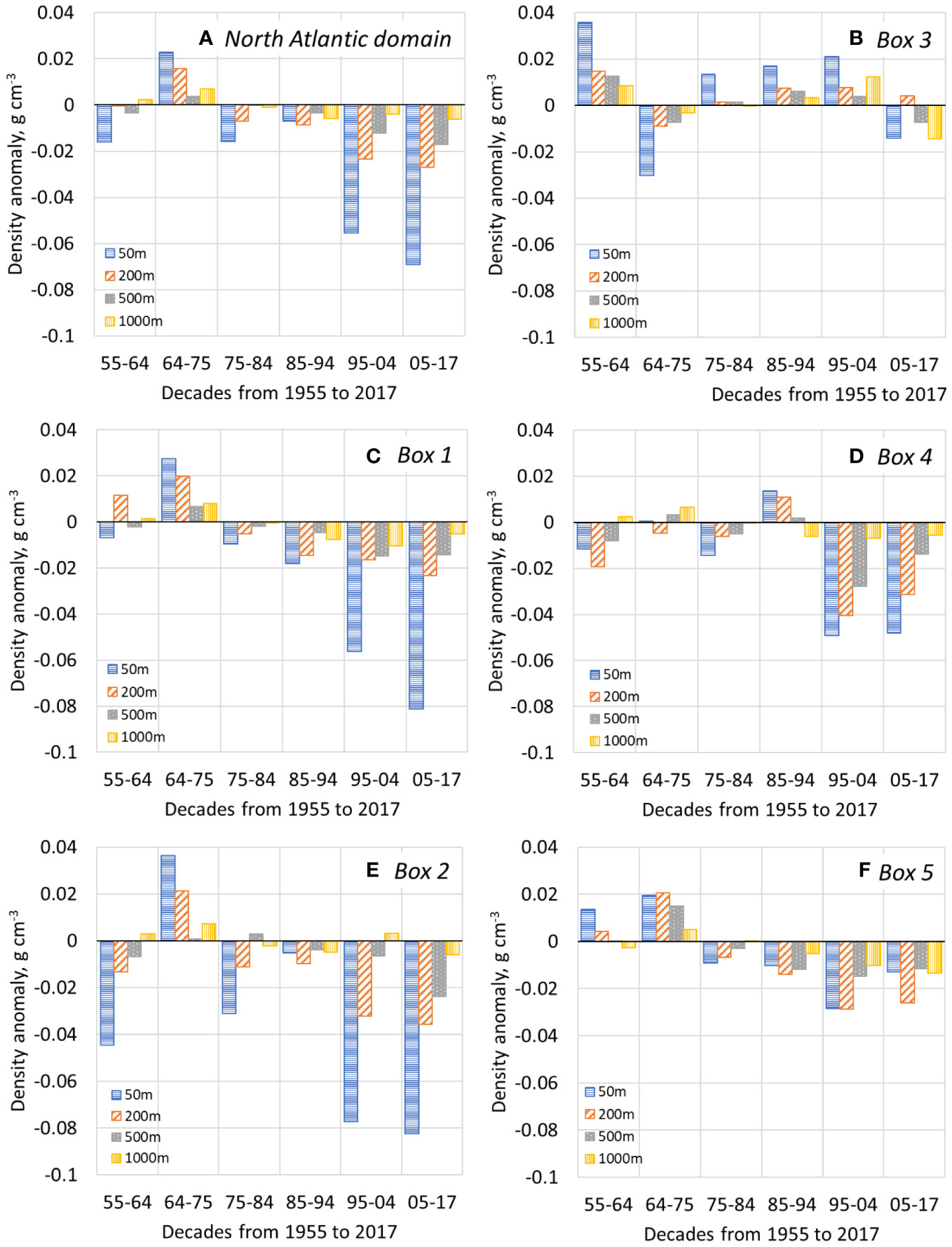
Figure 7 Decadal variability of the annual density anomalies at the different depth relative to the climate normals, i.e., the individual decades minus 1965–1994 climate normals: (A) in the entire North Atlantic; (B–F) in the selected boxes 1 through 5 shown in Figure 1. Vertical axis – (σ_t=ρ-1000 kg s^-1). Vertical axis – density anomalies; horizontal axis – decades.

In a preceding publication (Seidov et al., 2017), we discussed temperature and ocean heat content shifts in the NA in regions similarly approximated by the boxes in Figure 1. Here, the analysis of salinity and density is added to connect to possible causations of the suspected NA decadal circulation shifts. There is also an additional region embodying the Nordic Seas (Box 5) added, which may be important for the AMOC dynamics, e.g (Eldevik et al., 2009; Drange et al., 2013).

The plot in Figure 5A displays the temperature deviation from normals, which is the average temperature of the entire North Atlantic region. As per Figure 5A, the region has been experiencing a continuous temperature increase since 1965-1974. Additionally, Figure 6A indicates that the water in the region has also become saltier. It is important to note that for a given temperature, seawater tends to become denser when salinity increases. However, since density’s dependence is higher on temperature than salinity outside of the high latitudes (i.e., cold temperatures), the upper 1500 m in the NA is getting warmer and thus also becomes lighter (Figure 7A).

Although near-surface warming is more substantial than in deeper layers, the deep ocean is also warming, albeit much slower. However, these overall warming tendencies found in the NA are not experienced similarly by all subregions. Box 2 (Figure 5E; the eastern part of the subtropical gyre) and Box 5 (Figure 5F; Nordic Seas) reveal tendencies like those of Box 1 (Figure 5C; Gulf Stream). Box 3 (Figure 5B; Labrador Sea) and Box 4 (Figure 5D; the eastern part of the subpolar gyre dominated by the cold outflow from the Greenland Sea), experience radically different behavior. Box 1 demonstrates noticeably steep warming (Figure 5C) and salinization (Figure 6C) from 1965-1974. Boxes 2 and 5 and the entire NA have similar trends (Figures 5A, E, F, 6A, E, F). In the Labrador Sea, occupying most of Boxes 3 (Figure 5B), a warming trend did not begin until the 1985-1994 decade. The region within Box 4 (Figure 5D) is dominated by the cold East Greenland Current (EGC), East Greenland Coastal Current (EGCC), and Irminger Current. This region is only marginally impacted by the North Atlantic Drift in its most southeast part, east of the Reykjanes Ridge. Therefore, its thermal regime’s change resembles that of Box 3 (Figure 5B), to which Box 2 is connected via the cold West Greenland Current, a continuation of the outflow from the Greenland Sea. There is an essential difference between those two regions of the subpolar gyre—temperatures at the deeper layers in Box 4 (Figure 5D) began decreasing in the last decade (i.e., 2005-2017), while in Box 3 (Figure 5B) deep temperatures kept rising.

Despite the recent cooling of Box 4 (Figure 5D), Box 5 (Figure 5F, the Nordic Seas area) connected to Box 4 shows temperature changes most like Box 1 (Figure 5C, the Gulf Stream area) and Box 2 (Figure 5E, Azores Current area). We expect that it is due to the direct flow of the Gulf Stream water via the North Atlantic Drift through the southeastern part of Box 4 (Figure 5D) and the Azores Current (Box 2, Figure 5E). As was mentioned above, the northwestern part of Box 4 is mainly controlled by cold EGC and EGCC and the relatively cool Irminger Current (warm branch of the North Atlantic Drift mixing with EGC). Therefore, Box 4 reveals cooler trends than the subtropical gyre and the Nordic Seas, which are dominated by the warm Atlantic water inflow, e.g (Yashayaev and Seidov, 2015); see Figure 1. More detailed maps of surface currents in the Box 4 area can be viewed in (Sarafanov et al., 2012) and (Fontela et al., 2016). The southeastern part of Box 4 is the transit zone for the warm Atlantic water flowing toward the Nordic Seas.

It has recently been shown that the thermohaline and dynamic signal in the Azores Current correlates with the signal in the Gulf Stream with a lag of approximately two years (Frazão et al., 2022). This period is much shorter than the decadal averaging, which could explain the decadal similarity between Boxes 1 (Figure 5C) and 2 (Figure 5E). A similar connection exists between the Gulf Stream and the Norwegian Current where the warm Atlantic water enters the Nordic Seas (Yashayaev and Seidov, 2015). The early multidecadal cooling in Box 3 (Figure 5B), mostly occupied by the Labrador Sea, may be related to the cold currents flowing clockwise around Greenland. These cold currents, the EGC, EGCC, and the West Greenland Current, carry cold and fresh water from the Greenland Sea to the Labrador Sea. This may be the reason why there was cooling in the middle and western parts of the subpolar gyre when the remainder of the NA was warming.

We have already reported striking differences between climate change in the Gulf Stream and Labrador Current regions (Seidov et al., 2017). Still, our initial study lacked a combined temperature and salinity analysis. Salinity and density have quite similar tendencies in concert with temperature in all boxes (Figures 6, 7), though salinity changes primarily compensate (from a density perspective) for temperature changes. It agrees with model results showing that the NA warming is accompanied by an increase in salinity, e.g (Saba et al., 2016). Salinity in Boxes 3 and 4 (Figure 6B; Labrador Sea, and Figure 6D; Irminger Sea) is as different from the other three boxes as temperature. We argue that the radical difference between Boxes 3 and 4 and Boxes 1, 2, and 5 is because the subpolar gyre is dominated by upward Ekman pumping, bringing cold deep water to the surface, and because of the cold currents around Greenland, while Boxes 1 and 2 (the Gulf Stream and Azores currents areas) are comprised of the subtropical gyre and are dominated by downward Ekman pumping of the warm water. The line between the cold and fresh waters in Boxes 3 and 4 and warm and saline waters in Boxes 1 and 2 roughly follows the zero line of the WSC (Figure 2). The Nordic Seas (Box 5) is a standalone case because despite having upward Ekman pumping there, the Nordic Seas is overwhelmed by the Atlantic water inflow, and thus, in general, mimics Box 1 trend. The Atlantic Water intrusion into the Norwegian Sea also depends on the strength of those currents, and therefore, the changes in the Nordic Seas follow those in Boxes 1 and 2. There are lags in signal traveling across the Atlantic, but as discussed earlier, those lags are short (i.e., ~2 to 3 years) when compared to our decadal time scales (Frazão et al., 2022).

The salinization of seawater leads to density increase. However, because the temperature is high enough in the NA and all five boxes to govern the density, the latter followed temperature tendencies, and in the last two decades the ocean’s upper layers became noticeably lighter compared to the density normals (Figure 7). In three boxes (Boxes 1, 2, and 5) and the overall NA (Figures 7A, C, E, F), the density began decreasing concurrently with warming—from 1965-1974 and all the way up through 2005-2017. Decreasing of seawater density in Boxes 3 (Figure 7B) and 4 (Figure 7D) lagged the rest of the NA by two decades. Note that the salinity changes in the NA depend on both circulation and the hydrological cycle, i.e., evaporation minus precipitation over the NA. The NA intra-basin near-surface salinity contrast and intra-basin moisture transport are connected and may play an important role in maintaining the AMOC functionality (Reagan et al., 2018). However, we are not digging into this issue as it would further complicate our analysis and because the near surface in situ salinity already reflects the freshwater balance. What is important here, as Figures 6 and 7 imply, is that the near-surface salinity was reduced, but the near-surface density increased in Boxes 3 and 4 (Labrador and Irminger basins, respectively) between the 1975-1994 period because the near-surface temperature also decreased and overcompensated the near-surface freshening. Importantly, this densification of the new-surface water preceded the AMOC slowing in the last two decades.

Finally, to complete the analysis of the changes in the NA climate, water transports were computed across the vertical sections from the sea surface to 1500 m depth at 40°N (not shown) and 50°N (Figure 8). The transports were calculated using the D-velocity and T-velocity data (see Research Strategy and Methods). Figure 8 shows the northward water transport in the upper 1500 m in Sverdrups (1Sv=10⁶ m³s^-1). The northward water transport estimates are shown across the latitudinal section between the meridians 45°W and 20°W (Figure 8). The transports are estimated by integrating velocities at 50, 200, 500, and 1000 m from the sea surface to 1500 m using Equation 7. Since the T-velocities are from SODA, the earliest available decade for comparison to D-velocity transport is 1985-1994. The western edge of the sections is determined by the dynamic method calculation requiring the ocean depth to be greater than 1500 m. The portion of the latitudinal section at 50°N was selected in the area with predominant northward flows (see Figures 3A, B).

Figure 8

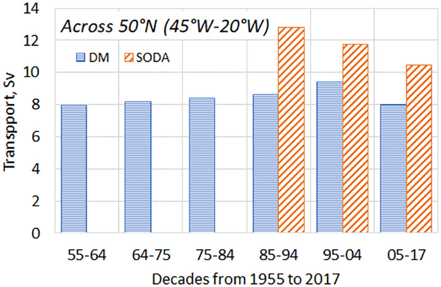
Figure 8 Decadal variability of the water transports (Sv) within 0-1500 m layer across 50°N between 45°W – 20°W calculated by dynamic method (blue bars) and SODA (orange bars). Vertical axis – water transport (Sv); horizontal axis – decades.

The transports in Figure 8 are consistent with those found in other transport assessments (Buckley and Marshall, 2016). There is no systematic decrease of the northward transport across the selected sections of the flow between the 1955-1964 and 1995-2004 decades. However, there is a clear decline of transport since 1985-1994 and 2005-2017 in SODA reanalysis.

We also estimated the eastward decadal water transport within the upper 1500 m across the section within the Gulf Stream along the 65°W meridian and between 35°N-43°N parallels (Figure 9). Figure 9 shows the eastward transport across the Gulf Stream continuation before it splits into the Azores Current and, after turning north, the North Atlantic Current. The northward transport shown in Figure 8 correlates well with the kinetic energy in Box 1, as Figure 10 reveals (compare Figures 8, 10), with the correlation coefficients 0.775 for D- and 0.848 for T-velocities.

Figure 9

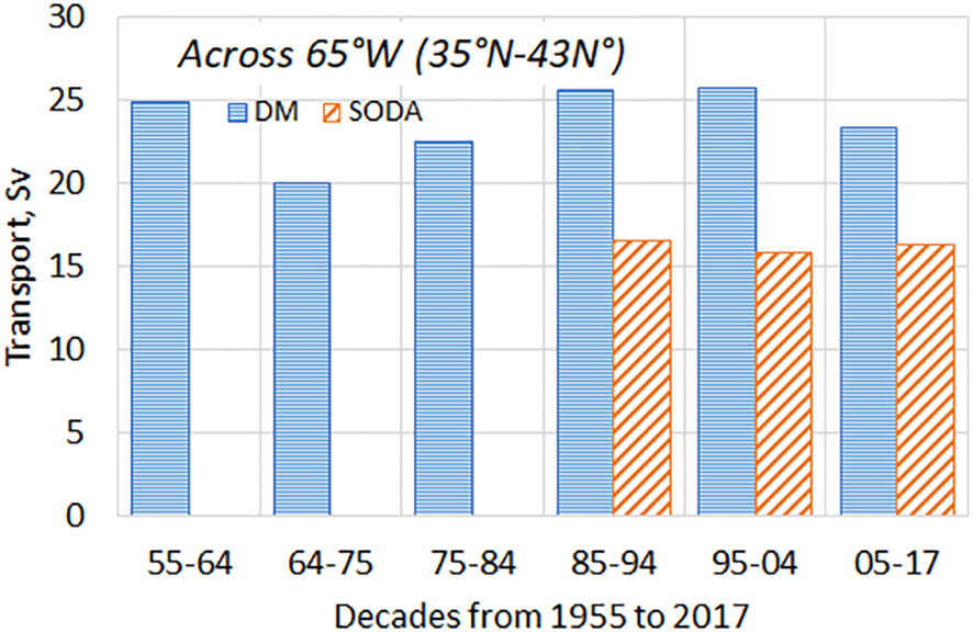
Figure 9 Decadal variability of the water transports (Sv) within the upper 1500 m layer across 65°W between 35°N – 43°N calculated by dynamic method (blue bars) and SODA (orange bars). Vertical axis – water transport (Sv); horizontal axis – decades.

Figure 10

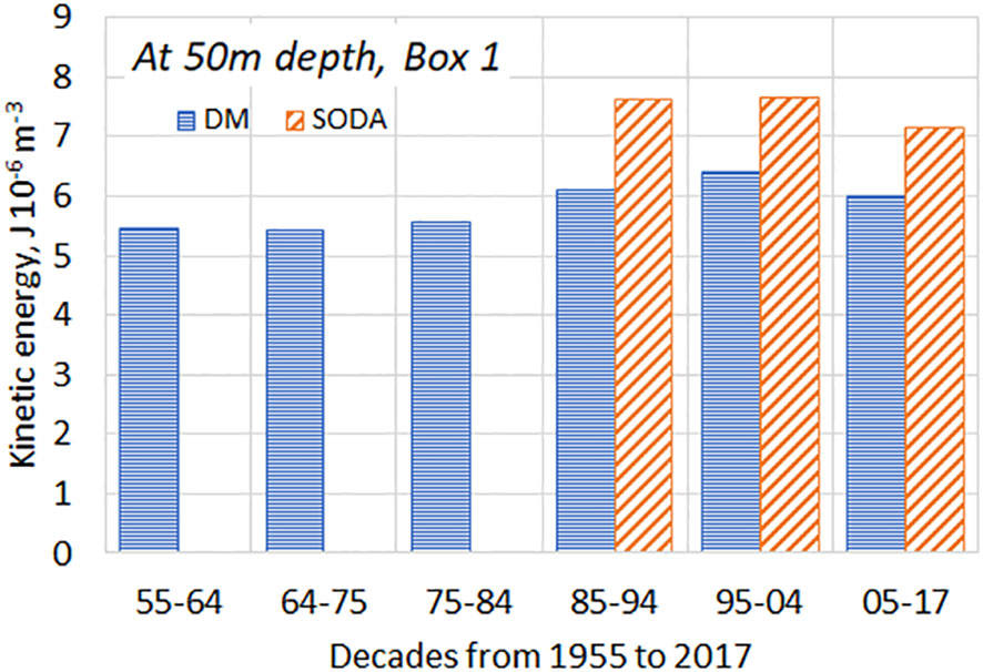
Figure 10 Decadal variability of the kinetic energy in Box 1 is calculated by the dynamic method (blue bars) and SODA (orange bars). Vertical axis – kinetic energy (J·10^-6m^-3); horizontal axis – decades.

The meridional water transports [Q_M in Equation (7)], in both D-velocity and T-velocity cases, are of the same order of magnitude, with T-velocity transport decreasing from 1985-1994 to 2005-2017 from ~12 Sv to ~10 Sv (Figure 8), while the D-velocity transport slightly increases from 8 Sv in the early decade of 1955-1964 to 9 Sv in 1995-2004 and then decreasing to less than 8 Sv in 2005-2017. Note, although the pattern and, in some cases, the intensity of the D- and T-velocities are similar (Figures 8, 9), a direct comparison between the two should be avoided since the D-velocities are computed relative to the level of no motion and only where the ocean is deeper than the depth of that level (i.e., 1500 m).

In contrast to the D-velocities, the T-velocities are not constrained by the limits of the dynamic method and can be calculated for most of the NA (see Research Strategy and Methods). However, the tendencies of the water transports and kinetic energy in Figures 8 and 9 are coherent in most places where both D- and T-velocities are computed.

In both cases, there is a noticeable decrease in the northward transport of warm and salty Gulf Stream water to the subpolar gyre and further to the Nordic Seas. However, the rise and fall of this transport is not severe. On the contrary, the maximum difference between the high transports in 1985-1994 and the lowest in 2005-2017 is only 20% (in the data from SODA in Figure 8; the dynamic method gives even smaller changes). Noteworthy, however, is the fact that both methods yield a slowing down of the upper arm of the AMOC and confirm that the AMOC upper limb is controlled by the Gulf Stream, which was shown to be resilient to ongoing upper ocean warming (Seidov et al., 2019b, Seidov et al., 2021).

Figure 11 shows the differences in the specific kinetic energy (computed using the T velocities) between the decades of 2005-2017 and 1985-1994 at 50-m (a) and 200-m depths (b). At both depths, the kinetic energy maps suggest that there is a substantial decrease of KE in the transition zone (the zone of the confluence of the Gulf Stream and Labrador Current). Generally, the kinetic energy in the entire upper ocean of the NA increased until 1995-2004 (Figure 10; Table 2), with noticeable decreases afterward. The decrease in KE in the last decade relative to 1985-1994 happens almost everywhere in the subtropical gyre, but especially in the transition zone and along the line where the northward AMOC upper-ocean transport is both maximal and most vulnerable, confirms that the AMOC was slowing down in the recent decades.

Figure 11

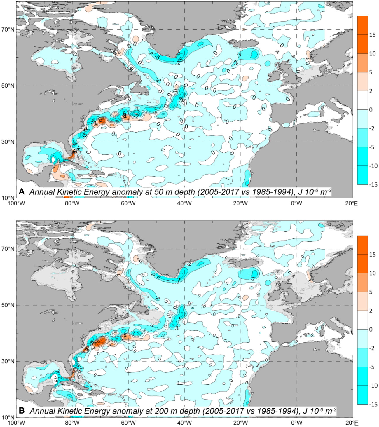
Figure 11 Differences of annual specific kinetic energy between 2005-2017 and 1985-1994 at (A) 50 m and (B) 200 m depths. Kinetic energy was calculated using T velocities; KE is in J·10^-6m^-3.

4 Discussion and conclusions

The results of quantifying the changes in ocean circulation, both in intensity and structure, confirm the conclusions from our previous work on the NA multidecadal variability and climate shift (Seidov et al., 2017). The ocean heat content in the cited publication in the four regions of the NA (approximately Boxes 1 through 4 in this study) and the temperature anomalies shown in Figure 5 look quite similar. The trends of salinity and density (Figures 6, 7), along with those of temperature, imply that the NA is split into two main parts—the Labrador Sea (Box 3), including the adjacent area of the western part of the subpolar gyre (northwestern part of Box 4), and the eastern part of the subpolar gyre (southeastern part of Box 4) coupled with the subtropical gyre (Boxes 1 and 2) and the Nordic Seas (Box 5) which is connected to Box 1 via the North Atlantic water intrusion into the Norwegian Sea (Yashayaev and Seidov, 2015).

We show that there are two climates—the western subpolar gyre climate, dominated by the cold currents (i.e., the EGC, EGCC, West Greenland, and Labrador currents), and the subtropical gyre climate, dominated by the Gulf Stream, North Atlantic Drift, and Azores currents. Furthermore, the Nordic Seas also exhibits similar variability as the subtropical gyre climate which may be explained by being directly connected to the subtropical gyre via the Norwegian Current.

It is also clear that the zero line of the WSC roughly separates these two climates approximated by a straight line in Figure 2, dissecting the two climates along a line generally following the water flow stemming from the Gulf Stream and continuing toward the British Isles as the North Atlantic Current and further as the North Atlantic Drift. As we previously argued (Seidov et al., 2019a), the Ekman pumping is responsible for the Eighteen Degree Water (EDW) heaving and thus accumulating disproportionally large amounts of OHC southeast of the Gulf Stream. It is argued to be the main stabilizing factor in the Gulf Stream resilience over multiple decades (Seidov et al., 2019b).

We also conclude that because the WSC did not significantly change structurally (Figure 2B), the only cause of the thermohaline circulation variability is the increase or decrease in density gradients maintained by the currents and Ekman pumping (Figure 2C). Density has continuously decreased in the subtropical gyre and the Nordic Seas since 1965-1974. Temperature and density changes in the subtropical gyre dominate the entire NA amid the different climate trajectories of the subpolar gyre (roughly separated from the subtropical gyre by the line of zero WSC, as shown in Figure 2). Based on previous findings (Seidov et al., 2017; Seidov et al., 2019b; Frazão et al., 2022), we argue that the Gulf Stream and its continuation dominates the climate of the subtropical gyre, the eastern part of the subpolar gyre, and the Nordic Seas (Yashayaev and Seidov, 2015).

However, the NA circulation and the Gulf Stream are resilient to the ongoing warming. First, the path of the Gulf Stream jet is a very stable (Seidov et al., 2019b) possessing a feature that can be characterized as a “stiffness” (Rossby, 1999; Rossby et al., 2014). Second, the Gulf Stream resilience is also due to the dampening effect of the EDW heaving and ocean heat content accumulation trapping within the EDW bowl (Seidov et al., 2019b). However, it was noticed that the amplitude of the latitudinal spread of the Gulf Stream Cold Wall annual position increased in the most recent decade of 2005-2017 without any significant deviation of the corresponding decadally averaged Gulf Stream pathway (Seidov et al., 2019b). This can be an additional factor of rather moderate variability of the water transport in the Gulf Stream extension (in the meridional section across 65°W) displayed in Figure 9.

The mild alteration of the flow patterns and intensity over the past six decades also demonstrates the overall resilience of the NA climate. The water transport and kinetic energy across the 50°N section reveal a definitive slowdown of the AMOC in the last decade and perhaps even since the late 1990s. Nonetheless, none of the climate parameters—temperature, salinity, density, transports, or kinetic energy differences between the decades suggest dramatic changes in the NA climate over the past 60 years. The only dissonances between AMOC changes and temperature (salinity, density) are: (i) the evident slowdown of the upper arm of the AMOC manifested in weakening the northward water transport within the upper 1500 m across 50°N in the last decade and (ii) continued warming everywhere in the NA, except the western part of the subpolar gyre. Therefore, echoing the recent discussion in (Seidov et al., 2021), we can argue that there is an indication that the current situation may not be entirely indicative of what the future may hold.

The results showing the Gulf Stream resilience do not imply that the situation will continue to be stable in the future. Indeed, in (Seidov et al., 2019b), we argued that the Gulf Stream’s influence over the AMOC on the decadal and longer timescales may stem from (a) strong decadal variability of the Gulf Stream volume transport (and thus kinetic energy) within a stiff and resilient jet between 75°W and 50°W (some authors debates this possibility), (b) wandering of the Gulf Stream extension and North Atlantic Current east of 50°W, or (c) some combination of the two. At the time of the analysis reported in (Seidov et al., 2019b), verifying whether this hypothesis holds was not viable because we did not consider the variability of density and velocity within the Gulf Stream system and based our arguments solely on temperature records. Now we have much greater confidence in the hypothesis that a combination or synergy of those two factors—variability in the transport or kinetic energy and wandering of the Gulf Stream extension—does play a combined role in possible AMOC slowing, as Figure 11 suggests.

A word of caution is needed here regarding the future of the NA circulation and climate tied to the AMOC dynamics. The decade of 2005–2017 has undergone an unprecedented northward excursion of warm near-surface Gulf Stream water in summer (Seidov et al., 2021), which may signal that the resilience of the Gulf Stream system is wading. There is no clear sign that this behavior will persist, further accelerate, or noticeably diminish in the next decade and beyond. Scenarios with a very serious slowdown or even a total collapse of the AMOC, such as in (Boers, 2021; Ditlevsen and Ditlevsen, 2023) and a few other studies, cannot be completely dismissed.

There is another aspect of the state of resilience of the Gulf Stream system. The last decade witnessed an “abnormal” behavior of the Gulf Stream, which did not occur during the previous 50 years. It manifested in accelerated warming of the Slope Water over the past decade (Seidov et al., 2021). Based on our analysis of the AMOC fingerprints—temperature, salinity, and density of the upper 1500 m—we cannot yet be sure that the NA ocean climate will remain resilient if it drifts towards a warmer and lighter upper ocean state. It is also unclear if a slower upper arm of the AMOC state will ignite less resilient and more fragile modes of the NA ocean climate. We also cannot be sure that the trends of sea surface temperature and density continue toward much warmer and lighter surface ocean water for the foreseeable future. Whether they do or not, the AMOC’s fate remains unclear. However, our analysis implies that the current North Atlantic Ocean circulation and climate remain relatively stable amid observed surface warming and possibly related recent AMOC slowing.

Data availability statement

Publicly available datasets were analyzed in this study. This data can be found here: https://www.ncei.noaa.gov/products/world-ocean-atlas and http://www.soda.umd.edu.

Author contributions

AM: Data curation, Formal analysis, Investigation, Software, Visualization, Writing – review & editing. DS: Conceptualization, Investigation, Methodology, Project administration, Resources, Supervision, Validation, Writing – original draft. JR: Data curation, Software, Validation, Writing – review & editing.

Funding

The author(s) declare financial support was received for the research, authorship, and/or publication of this article. This study was partially supported by NOAA grant NA19NES4320002 (Cooperative Institute for Satellite Earth System Studies -CISESS) at the University of Maryland/ESSIC. Further support was provided by NOAA’s Climate Program Office’s Ocean Observing and Monitoring Division.

Acknowledgments

We want to thank the scientists, technicians, data center staff, and data managers for their contributions of data to the IOC/IODE, ICSU/World Data System, and NOAA/NCEI Ocean Archive System, which provided a foundation of in situ oceanographic data for this work. We are especially thankful to Sydney Levitus (retired, formerly of NOAA/NCEI) for his pioneering work on the World Ocean Climatology that initiated all subsequent efforts in building WOD and all ocean climatologies founded on this database. We also thank our colleagues at NOAA/NCEI for many years of data processing and constructing the World Ocean Database and World Ocean Atlas and especially to Tim Boyer of NOAA/NCEI for his leadership role in the WOD project and to Kirsten Larsen of NOAA/NCEI for her support of the NCEI Regional Climatology and the first author’s work. We thank Scott Cross of NOAA/NCEI for his useful comments and suggestions. The scientific results and conclusions, as well as any views or opinions expressed herein, are those of the authors and do not necessarily reflect those of NOAA or the Department of Commerce.

Conflict of interest

The authors declare that the research was conducted in the absence of any commercial or financial relationships that could be construed as a potential conflict of interest.

Publisher’s note

All claims expressed in this article are solely those of the authors and do not necessarily represent those of their affiliated organizations, or those of the publisher, the editors and the reviewers. Any product that may be evaluated in this article, or claim that may be made by its manufacturer, is not guaranteed or endorsed by the publisher.

Author disclaimer

The views, opinions, and findings in this report are those of the authors and should not be construed as an official NOAA or US Government position, policy, or decision.

References

Behrens E., Biastoch A., Böning C. W. (2013). Spurious AMOC trends in global ocean sea-ice models related to subarctic freshwater forcing. Ocean Model. 69, 39–49. doi: 10.1016/j.ocemod.2013.05.004

CrossRef Full Text | Google Scholar

Bindoff N. L., McDougall T. J. (1994). Diagnosing climate change and ocean ventilation using hydrographic data. J. Phys. Oceanography 24, 1137–1152. doi: 10.1175/1520-0485(1994)024<1137:DCCAOV>2.0.CO;2

CrossRef Full Text | Google Scholar

Boers N. (2021). Observation-based early-warning signals for a collapse of the Atlantic Meridional Overturning Circulation. Nat. Climate Change 11, 680–688. doi: 10.1038/s41558-021-01097-4

CrossRef Full Text | Google Scholar

Bower A., Lozier S., Biastoch A., Drouin K., Foukal N., Furey H., et al. (2019). Lagrangian views of the pathways of the atlantic meridional overturning circulation. J. Geophysical Research: Oceans 124, 5313–5335. doi: 10.1029/2019JC015014

CrossRef Full Text | Google Scholar

Boyer T. P., Garcia H. E., Locarnini R. A., Zweng M. M., Mishonov A. V., Reagan J. R., et al. (2018). World ocean atlas 2018 (Silver Spring, MD, U.S.A.: NOAA/NESDIS).

Google Scholar

Bryden H. L., Longworth H. R., Cunningham S. A. (2005). Slowing of the Atlantic meridional overturning circulation at 25°N. Nature 438, 655–657. doi: 10.1038/nature04385.

PubMed Abstract | CrossRef Full Text | Google Scholar

Buckley M. W., Marshall J. (2016). Observations, inferences, and mechanisms of Atlantic Meridional Overturning Circulation variability: A review. Rev. Geophysics 54, 5–63. doi: 10.1002/2015RG000493

CrossRef Full Text | Google Scholar

Caesar L., Rahmstorf S., Robinson A., Feulner G., Saba V. (2018). Observed fingerprint of a weakening Atlantic Ocean overturning circulation. Nature 556, 191–196. doi: 10.1038/s41586-018-0006-5

PubMed Abstract | CrossRef Full Text | Google Scholar

Caínzos V., Hernández-Guerra A., McCarthy G. D., McDonagh E. L., Cubas Armas M., Pérez-Hernández M. D. (2022). Thirty years of GOSHIP and WOCE data: atlantic overturning of mass, heat, and freshwater transport. Geophysical Res. Lett. 49, e2021GL096527. doi: 10.1029/2021GL096527

CrossRef Full Text | Google Scholar

Carton J. A., Chepurin G. A., Chen L. (2018). SODA3: A new ocean climate reanalysis. J. Climate 31, 6967–6983. doi: 10.1175/JCLI-D-18-0149.1

CrossRef Full Text | Google Scholar

Chelton D. B., Schlax M. G., Freilich M. H., Milliff R. F. (2004). Satellite measurements reveal persistent small-scale features in ocean winds. Science 303, 978–983. doi: 10.1126/science.1091901

PubMed Abstract | CrossRef Full Text | Google Scholar

Chen C., Liu W., Wang G. (2019). Understanding the uncertainty in the 21st century dynamic sea level projections: the role of the AMOC. Geophysical Res. Lett. 46, 210–217. doi: 10.1029/2018GL080676

CrossRef Full Text | Google Scholar

Cheng W., Chiang J. C. H., Zhang D. (2013). Atlantic meridional overturning circulation (AMOC) in CMIP5 models: RCP and historical simulations. J. Climate 26, 7187–7197. doi: 10.1175/JCLI-D-12-00496.1

CrossRef Full Text | Google Scholar

Cheng L., von Schuckmann K., Abraham J. P., Trenberth K. E., Mann M. E., Zanna L., et al. (2022). Past and future ocean warming. Nat. Rev. Earth Environ. 3, 776–794. doi: 10.1038/s43017-022-00345-1

CrossRef Full Text | Google Scholar

Church J. A., Gregory J. M., Huybrechts P., Kuhn M., Lambeck K., Nhuan M. T., et al. (2001). “Changes in sea level,” in Climate change 2001: the scientific basis. Contribution of working group I to the third assessment report of the intergovernmental panel on climate change (Cambridge, UK: Cambridge University Press), 640–693.

Google Scholar

Couldrey M. P., Gregory J. M., Dong X., GAruba O., Haak H., Hu A., et al. (2023). Greenhouse-gas forced changes in the Atlantic meridional overturning circulation and related worldwide sea-level change. Climate Dynamics 60, 2003–2039. doi: 10.1007/s00382-022-06386-y

CrossRef Full Text | Google Scholar

Ditlevsen P., Ditlevsen S. (2023). Warning of a forthcoming collapse of the Atlantic meridional overturning circulation. Nat. Commun. 14, 4254–4265. doi: 10.1038/s41467-023-39810-w

PubMed Abstract | CrossRef Full Text | Google Scholar

Drange H., Dokken T., Furevik T., Gerdes R., Berger W., Nesje A., et al. (2013). “The nordic seas: an overview,” in The nordic seas: an integrated perspective (Washington, D.C., U.S.A.: American Geophysical Union), 1–10.

Google Scholar

Drijfhout S. (2015). Competition between global warming and an abrupt collapse of the AMOC in Earth’s energy imbalance. Sci. Rep. 5, 14877. doi: 10.1038/srep14877

PubMed Abstract | CrossRef Full Text | Google Scholar

Eldevik T., Nilsen J. E. O., Iovino D., Anders Olsson K., Sando A. B., Drange H. (2009). Observed sources and variability of Nordic seas overflow. Nat. Geosci 2, 406–410. doi: 10.1038/ngeo518.

CrossRef Full Text | Google Scholar

Fomin L. M. (1964). The dynamic method in oceanography (New York: Elsevier).

Google Scholar

Fontela M., García-Ibáñez M. I., Hansell D. A., Mercier H., Pérez F. F. (2016). Dissolved organic carbon in the North Atlantic meridional overturning circulation. Sci. Rep. 6, 26931. doi: 10.1038/srep26931

PubMed Abstract | CrossRef Full Text | Google Scholar

Frajka-Williams E., Ansorge I. J., Baehr J., Bryden H. L., Chidichimo M. P., Cunningham S. A., et al. (2019). Atlantic meridional overturning circulation: observed transport and variability. Front. Mar. Sci. 6. doi: 10.3389/fmars.2019.00260

CrossRef Full Text | Google Scholar

Frazão H. C., Prien R. D., Schulz-Bull D. E., Seidov D., Waniek J. J. (2022). The forgotten azores current: A long-term perspective. Front. Mar. Sci. 9. doi: 10.3389/fmars.2022.842251

PubMed Abstract | CrossRef Full Text | Google Scholar

Gill A. E. (1982). Atmosphere-ocean dynamics (New York: Academic Press).

Google Scholar

Greatbatch R. J., Fanning A. F., Goulding A. D., Levitus S. (1991). A diagnosis of interpentadal circulation changes in the North Atlantic. J. Geophysical Res. 96, 22009–22023. doi: 10.1029/91JC02423

CrossRef Full Text | Google Scholar

Häkkinen S., Rhines P. B., Worthen D. L. (2016). Warming of the global ocean: spatial structure and water-mass trends. J. Climate 29, 4949–4963. doi: 10.1175/JCLI-D-15-0607.1

CrossRef Full Text | Google Scholar

Hanawa K., Talley L. D. (2001). “Mode waters,” in Ocean circulation & climate: Observing and modelling the global ocean, Eds. Siedler G., Church J., Gould J. (New York: Academic Press), 373–386.

Google Scholar

Holland W. R., Hirschman A. D. (1972). A numerical calculation of the circulation in the North Atlantic Ocean. J. Phys. Oceanography 2, 336–354. doi: 10.1175/1520-0485(1972)002<0336:Ancotc>2.0.Co;2

CrossRef Full Text | Google Scholar

Hu A., Meehl G. A., Washington W. M., Dai A. (2004). Response of the atlantic thermohaline circulation to increased atmospheric CO2 in a coupled model. J. Climate 17, 4267–4279. doi: 10.1175/JCLI3208.1

CrossRef Full Text | Google Scholar

Huang R. X. (2015). Heaving modes in the world oceans. Climate Dynamics 45, 3563–3591. doi: 10.1007/s00382-015-2557-6

CrossRef Full Text | Google Scholar

IPCC. (2021). Climate change 2021: the physical science basis. Contribution of working group I to the sixth assessment report of the intergovernmental panel on climate change (Cambridge, United Kingdom and New York, NY, USA: Cambridge University Press).

Google Scholar

Jackson L. C., Biastoch A., Buckley M. W., Desbruyères D. G., Frajka-Williams E., Moat B., et al. (2022). The evolution of the North Atlantic Meridional Overturning Circulation since 1980. Nat. Rev. Earth Environ. 3, 241–254. doi: 10.1038/s43017-022-00263-2

CrossRef Full Text | Google Scholar

Jackson L. C., Wood R. A. (2020). Fingerprints for early detection of changes in the AMOC. J. Climate 33, 7027–7044. doi: 10.1175/JCLI-D-20-0034.1

CrossRef Full Text | Google Scholar

Johnson H. L., Cessi P., Marshall D. P., Schloesser F., Spall M. A. (2019). Recent contributions of theory to our understanding of the atlantic meridional overturning circulation. J. Geophysical Research: Oceans 124, 5376–5399. doi: 10.1029/2019JC015330

CrossRef Full Text | Google Scholar

Johnson G. C., Lumpkin R., Boyer T., Bringas F., Cetinić I., Chambers D. P., et al. (2022). Global oceans. Bull. Am. Meteorological Soc. 103, S143–S192. doi: 10.1175/BAMS-D-22-0072.1

CrossRef Full Text | Google Scholar

Johnson G. C., Lyman J. M. (2020). Warming trends increasingly dominate global ocean. Nat. Climate Change 10, 757–761. doi: 10.1038/s41558-020-0822-0

CrossRef Full Text | Google Scholar

Kuhlbrodt T., Griesel A., Montoya M., Levermann A., Hofmann M., Rahmstorf S. (2007). On the driving processes of the Atlantic meridional overturning circulation. Rev. Geophys. 45, RG2001. doi: 10.1029/2004RG000166

CrossRef Full Text | Google Scholar

Latif M., Roeckner E., Botzet M., Esch M., Haak H., Hagemann S., et al. (2004). Reconstructing, monitoring, and predicting multidecadal-scale changes in the North Atlantic thermohaline circulation with sea surface temperature. J. Climate 17, 1605–1614. doi: 10.1175/1520-0442(2004)017<1605:RMAPMC>2.0.CO;2

CrossRef Full Text | Google Scholar

Lee Y.-C., Liu W. (2023). The weakened atlantic meridional overturning circulation diminishes recent arctic sea ice loss. Geophysical Res. Lett. 50, e2023GL105929. doi: 10.1029/2023GL105929

CrossRef Full Text | Google Scholar

Levitus S., Antonov J. I., Boyer T. P., Baranova O. K., Garcia H. E., Locarnini R. A., et al. (2012). World ocean heat content and thermosteric sea level change (0–2000 m), 1955–2010. Geophys. Res. Lett. 39, L10603. doi: 10.1029/2012GL051106

CrossRef Full Text | Google Scholar

Lin Y.-J., Rose B. E. J., Hwang Y.-T. (2023). Mean state AMOC affects AMOC weakening through subsurface warming in the labrador sea. J. Climate 36, 3895–3915. doi: 10.1175/JCLI-D-22-0464.1

CrossRef Full Text | Google Scholar

Liu W., Fedorov A. (2022). Interaction between Arctic sea ice and the Atlantic meridional overturning circulation in a warming climate. Climate Dynamics 58, 1811–1827. doi: 10.1007/s00382-021-05993-5

CrossRef Full Text | Google Scholar

Liu W., Fedorov A., Sévellec F. (2019). The mechanisms of the atlantic meridional overturning circulation slowdown induced by arctic sea ice decline. J. Climate 32, 977–996. doi: 10.1175/JCLI-D-18-0231.1

CrossRef Full Text | Google Scholar

Liu W., Fedorov A. V., Xie S.-P., Hu S. (2020). Climate impacts of a weakened atlantic meridional overturning circulation in a warming climate. Sci. Adv. 6, eaaz4876. doi: 10.1126/sciadv.aaz4876

PubMed Abstract | CrossRef Full Text | Google Scholar

Liu W., Xie S.-P., Liu Z., Zhu J. (2017). Overlooked possibility of a collapsed atlantic meridional overturning Circulation in warming climate. Sci. Adv. 3, e1601666. doi: 10.1126/sciadv.1601666

PubMed Abstract | CrossRef Full Text | Google Scholar

Lozier M. S. (2012). Overturning in the North Atlantic. Annu. Rev. Mar. Sci. 4, 291–315. doi: 10.1146/annurev-marine-120710-100740.

CrossRef Full Text | Google Scholar

Mahajan S., Zhang R., Delworth T. L., Zhang S., Rosati A. J., Chang Y.-S. (2011). Predicting Atlantic meridional overturning circulation (AMOC) variations using subsurface and surface fingerprints. Deep Sea Res. Part II: Topical Stud. Oceanography 58, 1895–1903. doi: 10.1016/j.dsr2.2010.10.067

CrossRef Full Text | Google Scholar

Manabe S., Stouffer R. J. (1988). Two stable equilibria of a coupled ocean-atmosphere model. J. Climate 1, 841–866. doi: 10.1175/1520-0442(1988)001<0841:TSEOAC>2.0.CO;2

CrossRef Full Text | Google Scholar

Manabe S., Stouffer R. J. (1995). Simulation of abrupt change induced by freshwater input to the North Atlantic Ocean. Nature 378, 165–167. doi: 10.1038/378165a0.

CrossRef Full Text | Google Scholar

Marshall J., Plumb R. A. (2007). Atmosphere, ocean and climate dynamics: an introductory text (New York: Academic Press).

Google Scholar

McCartney M. S., Talley L. D. (1982). The subpolar mode water of the North Atlantic Ocean. J. Phys. Oceanography 12, 1169–1188. doi: 10.1175/1520-0485(1982)012<1169:tsmwot>2.0.co;2

CrossRef Full Text | Google Scholar

Mecking J. V., Drijfhout S. S., Jackson L. C., Graham T. (2016). Stable AMOC off state in an eddy-permitting coupled climate model. Clim. Dyn. 47, 2455–2470. doi: 10.1007/s00382-016-2975-0

CrossRef Full Text | Google Scholar

Megann A., Blaker A., Josey S., New A., Sinha B. (2021). Mechanisms for late 20th and early 21st century decadal AMOC variability. J. Geophysical Research: Oceans 126, e2021JC017865. doi: 10.1029/2021JC017865

CrossRef Full Text | Google Scholar

Mellor G. L., Mechoso C. R., Keto E. (1982). A diagnostic calculation of the general circulation of the Atlantic Ocean. Deep Sea Res. Part A. Oceanographic Res. Papers 29, 1171–1192. doi: 10.1016/0198-0149(82)90088-7

CrossRef Full Text | Google Scholar

Msadek R., Dixon K. W., Delworth T. L., Hurlin W. (2010). Assessing the predictability of the Atlantic meridional overturning circulation and associated fingerprints. Geophysical Res. Lett. 37, 19–24. doi: 10.1029/2010GL044517

CrossRef Full Text | Google Scholar

Pedlosky J. (1996). Ocean circulation theory (New York: Springer). doi: 10.1007/978-3-662-03204-6.

CrossRef Full Text | Google Scholar

Rahmstorf S. (1994). Rapid climate transitions in a coupled ocean-atmosphere model. Nature 372, 82–85. doi: 10.1038/372082a0.

CrossRef Full Text | Google Scholar

Rahmstorf S. (1995). Bifurcations of the Atlantic thermohaline circulation in response to changes in the hydrological cycle. Nature 378, 145–149. doi: 10.1038/378145a0.

CrossRef Full Text | Google Scholar

Rahmstorf S., Box J. E., Feulner G., Mann M. E., Robinson A., Rutherford S., et al. (2015). Exceptional twentieth-century slowdown in Atlantic Ocean overturning circulation. Nat. Climate Change 5, 475–480. doi: 10.1038/nclimate2554

CrossRef Full Text | Google Scholar

Reagan J., Seidov D., Boyer T. (2018). Water vapor transfer and near-surface salinity contrasts in the North Atlantic Ocean. Sci. Rep. 8, 8830. doi: 10.1038/s41598-018-27052-6

PubMed Abstract | CrossRef Full Text | Google Scholar

Reverdin G., Niiler P. P., Valdimarsson H. (2003). North Atlantic Ocean surface currents. J. Geophysical Research: Oceans 108, 2–1-2-21. doi: 10.1029/2001JC001020

CrossRef Full Text | Google Scholar

Rhein M., Mertens C., Roessler A. (2019). Observed transport decline at 47°N, Western Atlantic. J. Geophysical Research: Oceans 124, 4875–4890. doi: 10.1029/2019JC014993

CrossRef Full Text | Google Scholar

Richardson P. L. (2001). “Florida current, gulf stream, and labrador current,” in Encyclopedia of ocean sciences, Ed. Steele J. H. (Amsterdam: Elsevier Ltd), 1054–1064.

Google Scholar

Rossby T. (1999). On gyre interactions. Deep Sea Res. Part II: Topical Stud. Oceanography 46, 139–164. doi: 10.1016/S0967-0645(98)00095-2

CrossRef Full Text | Google Scholar

Rossby T., Flagg C. N., Donohue K., Sanchez-Franks A., Lillibridge J. (2014). On the long-term stability of Gulf Stream transport based on 20 years of direct measurements. Geophysical Res. Lett. 41, 2013GL058636. doi: 10.1002/2013GL058636

CrossRef Full Text | Google Scholar

Saba V. S., Griffies S. M., Anderson W. G., Winton M., Alexander M. A., Delworth T. L., et al. (2016). Enhanced warming of the Northwest Atlantic Ocean under climate change. J. Geophysical Research: Oceans 121, 118–132. doi: 10.1002/2015JC011346

CrossRef Full Text | Google Scholar

Sarafanov A., Falina A., Mercier H., Sokov A., Lherminier P., Gourcuff C., et al. (2012). Mean full-depth summer circulation and transports at the northern periphery of the Atlantic Ocean in the 2000s. J. Geophys. Res. 117, C01014. doi: 10.1029/2011JC007572

CrossRef Full Text | Google Scholar

Sarkisyan A. (1977). “"The diagnostic calculations of a large-scale oceanic circulation,",” in The sea, vol. 6 . Eds. Goldberg E. D., McCave I. N., O’Brien J. J., Steele J. H. (Wiley, New York), 363–458.

Google Scholar

Sarkisyan A. S., Sündermann J. (2009). Modelling ocean climate variability (Dordrecht, Netherlands: Springer). doi: 10.1007/978-1-4020-9208-4.

CrossRef Full Text | Google Scholar

Schmitz W. J. Jr. (1995). On the interbasin-scale thermohaline circulation. Rev. Geophysics 33, 151–173. doi: 10.1029/95RG00879.

CrossRef Full Text | Google Scholar

Schmitz W. J. Jr., McCartney M. S. (1993). On the North Atlantic circulation. Rev. Geophysics 31, 29–49. doi: 10.1029/92RG02583.

CrossRef Full Text | Google Scholar

Seidov D., Mishonov A. V., Baranova O. K., Boyer T. P., Nyadjro E., Bouchard C., et al. (2022). Northwest Atlantic Regional Ocean climatology version 2, (Silver Spring, MD, U.S.A.: NOAA Atlas NESDIS 88), 75 pp. doi: 10.25923/c6fz-fp67

CrossRef Full Text | Google Scholar

Seidov D., Mishonov A., Parsons R. (2021). Recent warming and decadal variability of gulf of maine and slope water. Limnology Oceanography 66, 3472–3488. doi: 10.1002/lno.11892

CrossRef Full Text | Google Scholar

Seidov D., Mishonov A., Reagan J., Parsons R. (2017). Multidecadal variability and climate shift in the North Atlantic Ocean. Geophysical Res. Lett. 44, 4985–4993. doi: 10.1002/2017GL073644

CrossRef Full Text | Google Scholar

Seidov D., Mishonov A., Reagan J., Parsons R. (2019a). Eddy-resolving in situ ocean climatologies of temperature and salinity in the Northwest Atlantic Ocean. J. Geophysical Research: Oceans 124, 41–58. doi: 10.1029/2018JC014548

CrossRef Full Text | Google Scholar

Seidov D., Mishonov A., Reagan J., Parsons R. (2019b). Resilience of the Gulf Stream path on decadal and longer timescales. Sci. Rep. 9, 11549. doi: 10.1038/s41598-019-48011-9

PubMed Abstract | CrossRef Full Text | Google Scholar

Seidov D., Stouffer R. J., Haupt B. J. (2005). Is there a simple bi-polar ocean seesaw? Global Planetary Change 49, 19–27. doi: 10.1016/j.gloplacha.2005.05.001.

CrossRef Full Text | Google Scholar

Sévellec F., Fedorov A. V. (2016). AMOC sensitivity to surface buoyancy fluxes: stronger Ocean meridional heat transport with a weaker volume transport? Climate Dynamics 47, 1497–1513. doi: 10.1007/s00382-015-2915-4

CrossRef Full Text | Google Scholar

Smeed D. A., Josey S. A., Beaulieu C., Johns W. E., Moat B. I., Frajka-Williams E., et al. (2018). The North Atlantic Ocean is in a state of reduced overturning. Geophysical Res. Lett. 45, 1527–1533. doi: 10.1002/2017GL076350

CrossRef Full Text | Google Scholar

Srokosz M., Baringer M., Bryden H., Cunningham S., Delworth T., Lozier S., et al. (2012). Past, present, and future changes in the atlantic meridional overturning circulation. Bull. Am. Meteorological Soc. 93, 1663–1676. doi: 10.1175/BAMS-D-11-00151.1

CrossRef Full Text | Google Scholar

Stouffer R. J., Seidov D., Haupt B. J. (2007). Climate response to external sources of freshwater: North Atlantic versus the Southern Ocean. J. Climate 20, 436–448. doi: 10.1175/JCLI4015.1.

CrossRef Full Text | Google Scholar

Talley L., Raymer M. (1982). Eighteen degree water variability. J. Mar. Res. 40, 757–775. Available at: https://elischolar.library.yale.edu/journal_of_marine_research/1666.

Google Scholar

Thorpe R. B., Gregory J. M., Johns T. C., Wood R. A., Mitchell J. F. B. (2001). Mechanisms determining the atlantic thermohaline circulation response to greenhouse gas forcing in a non-flux-adjusted coupled climate model. J. Climate 14, 3102–3116. doi: 10.1175/1520-0442(2001)014<3102:MDTATC>2.0.CO;2

CrossRef Full Text | Google Scholar

Timmermann A., Goosse H. (2004). Is the wind stress forcing essential for the meridional overturning circulation? Geophysical Res. Lett. 31, L04303. doi: 10.1029/2003GL018777

CrossRef Full Text | Google Scholar

Toggweiler J. R., Russell J. (2008). Ocean circulation in a warming climate. Nature 451, 286–288. doi: 10.1038/nature06590.

PubMed Abstract | CrossRef Full Text | Google Scholar

Weijer W., Cheng W., Drijfhout S. S., Fedorov A. V., Hu A., Jackson L. C., et al. (2019). Stability of the atlantic meridional overturning circulation: A review and synthesis. J. Geophysical Research: Oceans 124, 5336–5375. doi: 10.1029/2019JC015083

CrossRef Full Text | Google Scholar

WMO (2018). World meteorological organization: guide to climatological practices (Geneva, Switzerland: WMO).

Google Scholar

Yashayaev I., Seidov D. (2015). The role of the Atlantic Water in multidecadal ocean variability in the Nordic and Barents Seas. Prog. Oceanography 132, 68–127. doi: 10.1016/j.pocean.2014.11.009

CrossRef Full Text | Google Scholar

Yashayaev I., Seidov D., Demirov E. (2015). A new collective view of oceanography of the Arctic and North Atlantic basins. Prog. Oceanography 132, 1–21. doi: 10.1016/j.pocean.2014.12.012

CrossRef Full Text | Google Scholar

Zhang R. (2008). Coherent surface-subsurface fingerprint of the Atlantic meridional overturning circulation. Geophys. Res. Lett. 35, L20705. doi: 10.1029/2008GL035463

CrossRef Full Text | Google Scholar

Zhang R., Sutton R., Danabasoglu G., Kwon Y.-O., Marsh R., Yeager S. G., et al. (2019). A review of the role of the atlantic meridional overturning circulation in atlantic multidecadal variability and associated climate impacts. Rev. Geophysics 57, 316–375. doi: 10.1029/2019RG000644

CrossRef Full Text | Google Scholar

Zhu J., Liu Z., Zhang J., Liu W. (2015). AMOC response to global warming: dependence on the background climate and response timescale. Climate Dynamics 44, 3449–3468. doi: 10.1007/s00382-014-2165-x

CrossRef Full Text | Google Scholar

Zhu C., Liu Z., Zhang S., Wu L. (2023). Likely accelerated weakening of Atlantic overturning circulation emerges in optimal salinity fingerprint. Nat. Commun. 14, 1245. doi: 10.1038/s41467-023-36288-4

PubMed Abstract | CrossRef Full Text | Google Scholar

Zika J. D., Gregory J. M., McDonagh E. L., Marzocchi A., Clement L. (2021). Recent water mass changes reveal mechanisms of ocean warming. J. Climate 34, 3461–3479. doi: 10.1175/JCLI-D-20-0355.1

CrossRef Full Text | Google Scholar