Dynamic typhoon visualization based on the integration of vector and scalar fields

1 Introduction

As a result of the rapid changes in the global climate in recent years, many countries have experienced frequent disasters caused by extreme weather, resulting in significant loss of human and material resources (Li, 2022). Among them, typhoons are one of the most frequent and destructive meteorological disasters in the world, this cyclonic system, known for its powerful winds, torrential rains, and sea waves, poses a great threat and loss to many countries and is one of the global problems that mankind has to face for its survival and development nowadays (Xie et al., 2021; Chen et al., 2023). China is one of the countries in the world that are seriously affected by typhoons (Jiwei, 2023), and the northern part of the South China Sea, the Taiwan Strait, Taiwan Province, and its eastern coast, the western part of the East China Sea, and the Yellow Sea are all high-frequency zones through which typhoons pass, posing a serious threat to China’s social and economic development (Sui and Tang, 2015). To reduce the losses caused by disasters and to ensure the stable life of hundreds of millions of people and the steady development of society, it is crucial to carry out disaster prevention and mitigation of typhoons and other extreme weather (Guihua, 2017; Xina, 2017). Meteorological departments at all levels should closely monitor the movement of typhoons, issue timely monitoring and warning information on typhoons, make forecasts of future trends, and put forward specific analyses and forecasts of typhoon development trends, emphasizing the importance of typhoon meteorological monitoring, analyses, and forecasts (Lin et al., 2023; Yasir et al., 2024).

The visualization and analysis of typhoon is an important part of typhoon forecasting and prediction, strengthening the effect of typhoon visualization and analysis, improving the ability to utilize typhoon observation data, converting abstract typhoon meteorological data, drawing typhoon patterns and their spatial and temporal changes on the screen. It can help people understand the evolutionary pattern of typhoons and formulate precautionary measures, which is of great practical significance for disaster prevention and mitigation work in extreme weather, such as typhoons, and for rationalizing water resources (Lu et al., 2024). However, the typhoon is a complex vortex, and typhoons in different regions and at different moments have their uniqueness, which increases the difficulty of typhoon data processing and visualization of typhoon elements (Wanwan, 2023).

To effectively solve the problems of the typhoon’s many elements and the difficulty of visualization, this study is carried out with the multi-factor collaborative visualization of typhoon data. Since the proposal of scientific computing visualization, it has been widely used and developed in many fields such as geography, medicine, architecture, etc (Kehrer and Hauser, 2013), the scientific computing visualization of typhoon data presents the typhoon observation data and the data obtained in the process of scientific computation on the screen in the form of images or graphs (Zirui, 2020), which makes it convenient for researchers to interact, process, and analyze. The multi-dimensional, large-scale, complex structure and other characteristics of the current typhoon data make the traditional two-dimensional visualization methods not able to meet the demand for accurate expression of the typhoon, the need to take three-dimensional dynamic visualization techniques, such as volume data drawing, three-dimensional particle system, etc., the use of graphics processing unit(GPU) acceleration to improve the efficiency of the visualization of data (Li et al., 2023), to be able to characterize the morphology of the typhoon in a three-dimensional environment and its spatial-temporal evolution of the law. Dissecting the internal structure of typhoon data (Hao, 2020), predicting the movement and influence range of the typhoon, facilitating meteorologists to summarize the meteorological laws of the current typhoon, assisting in the decision-making of typhoon warning and personnel evacuation, and contributing to the cause of disaster prevention and mitigation.

Although existing research has made many improvements to the visualization of typhoons, the multi-dimensional, large-scale, and complex structure of the current typhoon remote sensing data makes the traditional visualization methods unable to meet the demand for an accurate representation of the typhoon (Yasir et al., 2023). To characterize the morphology of typhoons and their spatial and temporal evolution patterns in a three-dimensional environment, and to analyze the internal structure of typhoon data, it is convenient for meteorologists to summarize the meteorological laws of the current typhoon, to assist in the decision-making of typhoon warnings and evacuation of personnel, and to contribute to the cause of disaster prevention and mitigation, this study adopts the render volume method and particle system method for the visualization of typhoon volume data to realize the integration of vector and scalar fields of typhoon for dynamic visualization. The important contributions of this paper are listed below.

A volume rendering method based on the ray casting method is used, a hybrid interpolation method is proposed to accelerate the sampling time, and the Sobel operator is combined with the edge enhancement of the visualization effect to visualize the wind speed of the typhoon.

Realizes a particle system based on Web Graphics Library (WebGL), divides the calculation of massive particles into two parts: particle parallel tracking and particle dynamic rendering and implements a particle trace calculation method based on Lagrangian field to achieve the dynamic rendering of typhoon wind direction.

Based on the frame caching technique to achieve the fusion of the visualization effect of volume rendering and the visualization effect of particle system, the correct occlusion relationship is derived by calculating the blending color during rendering through the depth texture.

2 Related work

2.1 Volume rendering of scalar fields

Volume rendering is a scalar field visualization method, a technique that presents all the volume details simultaneously on a two-dimensional screen based on three-dimensional volume data. In the field of marine meteorology, scalar field visualization is the process of converting relevant scalar field data in meteorology (e.g., temperature, barometric pressure, humidity, etc.) into a visual form. Volume rendering is capable of sampling and synthesizing three-dimensional(3D) volume data directly and displaying different components and details inside the volume data by setting opacity values. Based on the condition of whether or not intermediate elements are required, volume rendering techniques can be categorized into two ways, which are direct volume rendering and indirect volume rendering techniques (Mady and Seoud, 2020).

Because the ray casting algorithm can yield high-quality rendering and has good parallelism, it has become the most popular volume rendering algorithm. Its principle is shown in Figure 1. The ray casting method is a direct volume rendering method based on physical ray simulation, proposed by Levoy in 1987, the algorithm is simple in principle, easy to realize perspective projection, and the quality of the rendered image is better (Zhang and Yuan, 2018).

Figure 1

Figure 1 Schematic of ray casting.

To accelerate the calculation speed of the ray casting method and improve its visualization effect, scholars at home and abroad have carried out in-depth research and improvement on it. Lee et al. ( 2010) proposed a fast ray casting algorithm that uniformly reconstructs the intensity values using a high-order convolution filter as the rays pass through the volume data, which reduces the number of sampling points as well as the computation steps for the color of the sampling points, and increases the sampling rate (Zanarini et al., 1998) proposed an optimization algorithm for the early cutoff of opacity, where the opacity iterates to 1 when the opacity stops subsequent sampling, eliminating invalid sampling and increasing sampling efficiency (Li et al., 2023) proposed an adaptive step-size sampling algorithm that arranges each layer in volume data according to its depth, shrinks the sampling step size for denser regions of data, increases the sampling points to obtain detailed information about the region of data changes, and increases the sampling step size for sparse regions of data to accelerate the sampling step. Chi (2012) proposed an adaptive multiple pre-integrated volume rendering algorithm. Firstly, the scalar values and positions of the sampling points on the sampling section are calculated, and the directional derivatives between the inlet and outlet points of the sampling section are obtained, further, the mutation positions of the transfer function on the sampling section are obtained, and the sampling step size is reduced proportionally according to the information of these positions. Meanwhile, some scholars optimized the computational efficiency of the ray casting algorithm, Lachlan J. Deakin et al. (Deakin and Knackstedt, 2020) computed the occupancy map of the data in the cube and the distance map between the data in advance by using the volume data, accelerating the speed of the light passing through the blank area in the cube, and reducing the sampling time (Li et al., 2011) proposed an octree-based dynamic volume rendering method that can visualize a large range of meteorological data.

2.2 Rendering of vector fields

Visualizing large-scale vector marine meteorological data can intuitively show the spatial and temporal changes of meteorology, which helps scholars to understand and predict weather conditions, and also has important applications for aviation, marine, and agriculture. However, vector field visualization of large-scale data is a very challenging application, and its excellent visualization effect needs the support of higher-performance computer hardware and software environment. Different visualization methods are often used to visualize data in different ways, and the appropriate method can make the best use of its strengths and avoid its weaknesses to present the data as well as possible. particle systems have emerged because of their unique advantages in imitating natural phenomena and physical phenomena, and have been widely used and researched.

Particle systems, first proposed by Reeves (Reeves, 1983), are based on the basic idea of modeling fuzzy irregular objects using a large number of particles with specific properties, randomly distributed and in constant motion, and continuously and dynamically plotting the motion state of a set of particles, which has been widely used in the representation of vector fields. The structure of the particle system is shown in Figure 2, in which each particle undergoes the three processes of generation, movement, and extinction, and a large number of particles carry out the three processes together to simulate the concrete form and movement characteristics of the abstract vector field. The particles are generated by the random point function, and get the initialized size, speed, direction, and other attribute information from the data, and continuously calculate the motion state of the next moment during the motion, and the particles that meet the extinction conditions will stop moving and be removed from the scene.

Figure 2

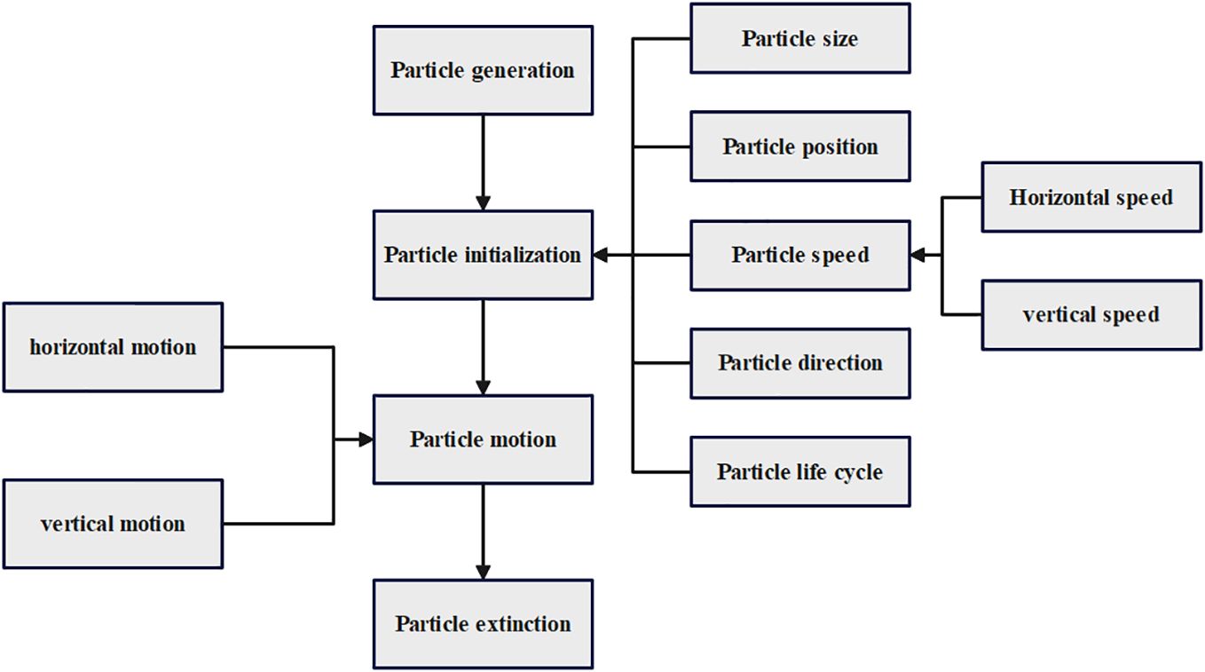
Figure 2 The structural composition of a particle system.

In the application of particle systems, many scholars have studied and improved it. Qian et al. (2005) dynamically reflect the wind field velocity direction as well as size through the position change of particles, and at the same time map the strength of the wind field vorticity into the rotational state of the particles themselves, and use algorithmic acceleration technology to visually represent the changing characteristics of the three-dimensional wind field. Shuai (2020) constructed a particle management system, and from the optimization of the particle system data structure, designed a three-layer structure of view volume index, flow field data grid, and particles, to quickly retrieve and render the particles in the current view volume, which greatly reduces the volume of particle visualization calculations, and improves the efficiency of the particle system to simulate the flow field (Shi et al., 2021) proposed a new method to visualize multilevel flow field dynamics based on a particle system, researched parallel particle tracking and efficient rendering, and proposed a viewport adaptive tuning algorithm that can efficiently express vector field features in multiscale situations (Zhang et al., 2019) computed the differences between the data at adjacent time points in different frames to change the attributes and introduced a Compute Unified Device Architecture (CUDA) parallel computing model to visualize large-scale particle changes, which reduced the Central Processing Unit (CPU) load and significantly improved the frame rate (Dai et al., 2023) used the smooth particle hydrodynamics (SPH) method to simulate the free surface problem in ocean engineering and reproduced the whole process of submarine landslide propagation and tsunami occurrence.

However, with the current particle system visualization technology, more research still stays on the single-moment two-dimensional expression effect. Vector data such as wind fields in the real world, characterized by multiple sources, multiple scales, and multiple dimensions, are in the process of constant spatial and temporal changes. With the change of time dimension, the direction and value of vector data change dynamically; with the improvement of observation equipment, the data height or depth level increases. The scale and complexity of vector data have gradually increased, and the demand for time-varying 3D visualization has also gradually increased. The current traditional two-dimensional Euler field particle system can only achieve the expression of multi-dimensional data by reloading the data of the next moment or the next level, which greatly increases the computational complexity, and the visualization is not coherent, and it cannot express the vector field changes in the three-dimensional scene. To express and convey the rich information contained in the wind field, more effective visualization and analysis tools and graphical algorithms are needed, and there is an increasing demand for high-performance, multi-scale, multi-dimensional, and time-varying visualization technological tools.

3 Proposed improved methodology

3.1 Scalar field visualization based on ray-casting method

3.1.1 GPU-based ray casting algorithm implementation

The ray-casting algorithm simulates the propagation and interaction of light rays in the scene by tracing the path of the rays to calculate the final color value. The principle of the algorithm is to emit a ray from the current viewpoint or observer position along the direction of each pixel, if the ray intersects with an object, the incidence point, the egress point, and the direction of the ray are calculated, the part of the ray located inside the volume data is sampled at equal distances and assigned a color value, and the color value of each pixel is synthesized with opacity into the final image, which is outputted to the screen.

This study implements a GPU-based ray casting algorithm based on WebGL, in which the vertex shader is responsible for processing the data enclosing the box and the coordinate transformation at the sampling points, and passes the coordinate information to the fragment shader, the specific flow is shown in the Figure 3. In the fragment shader, ray casting direction and distance calculation, texture resampling, and image synthesis are performed according to the acquired vertex information. The process is as follows:

Figure 3

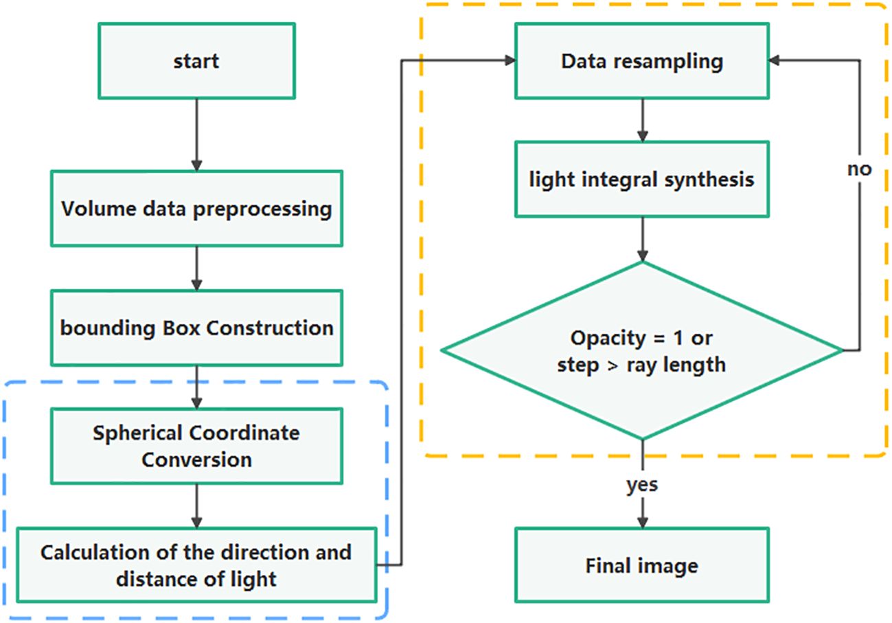
Figure 3 Ray casting Algorithm Flow.

Figure 4

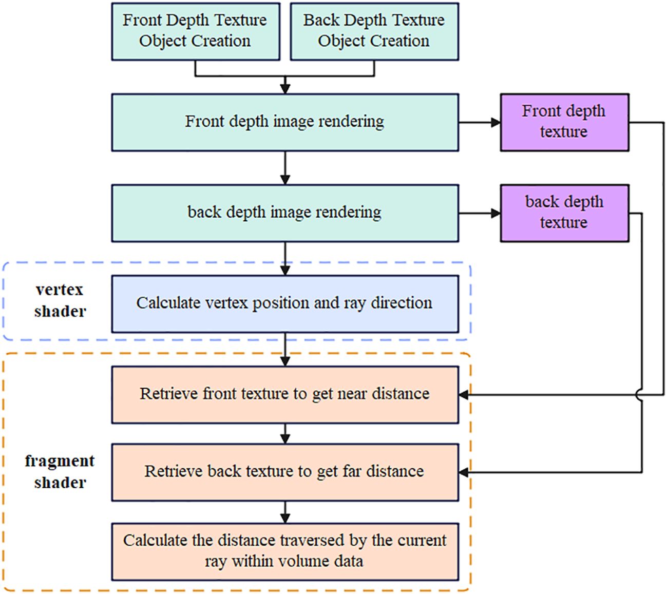
Figure 4 Light direction and distance calculation process.

1) Calculation of the direction and distance of ray casting.

In the volume rendering process, a bounding box is initially constructed to determine the final rendering. If the bounding box identifies that a voxel is not empty, the intersection points of the light ray with the data bounding box, i.e., the starting and ending points of the light ray, must be determined before texture resampling. This is essential for calculating the direction and length of the light ray. GPU-based volume rendering methods typically employ off-screen rendering and frame buffer object technology as is shown in Figure 4. The specific process involves:

① Generating a front depth texture object and a back-depth texture object to store the front and back depth information of the bounding box, respectively.

② Enabling the depth culling function in WebGL for front-side culling, rendering the data bounding box, and storing the back-side texture in the created back-side depth texture object.

③ Enabling the depth culling function in WebGL for back-side culling, rendering the data bounding box, and storing the front-side texture in the created front-side depth texture object.

Through the steps mentioned above, the color values stored in the front depth texture object and the back depth texture object are read to obtain the coordinates of the entry and exit points of the light. The distance and direction of the current light are then determined by subtracting these coordinates.

2) Texture Resampling

The ray casting method achieves volume rendering by uniformly sampling data at intervals throughout the 3D dataset through which the light passes. It blends the colors of sample points to determine the final displayed color for the current pixel. However, the typhoon volume data, stored in a grid format, is discrete in nature. Direct texture resampling won’t yield continuous rendering. Therefore, an interpolation function is introduced in the sampling process to convert the discrete data into continuous data.

This study utilizes the trilinear interpolation algorithm for interpolating three-dimensional discrete data as the interpolation function during the sampling process (Schulze and Lang, 2003). Its interpolation results typically do not exhibit significant deviations. The schematic of trilinear interpolation is depicted in Figure 5, and the interpolation value for the sampling point C(i,j,k) is related to its eight neighboring pixels as described in the following Equation 1:

Figure 5

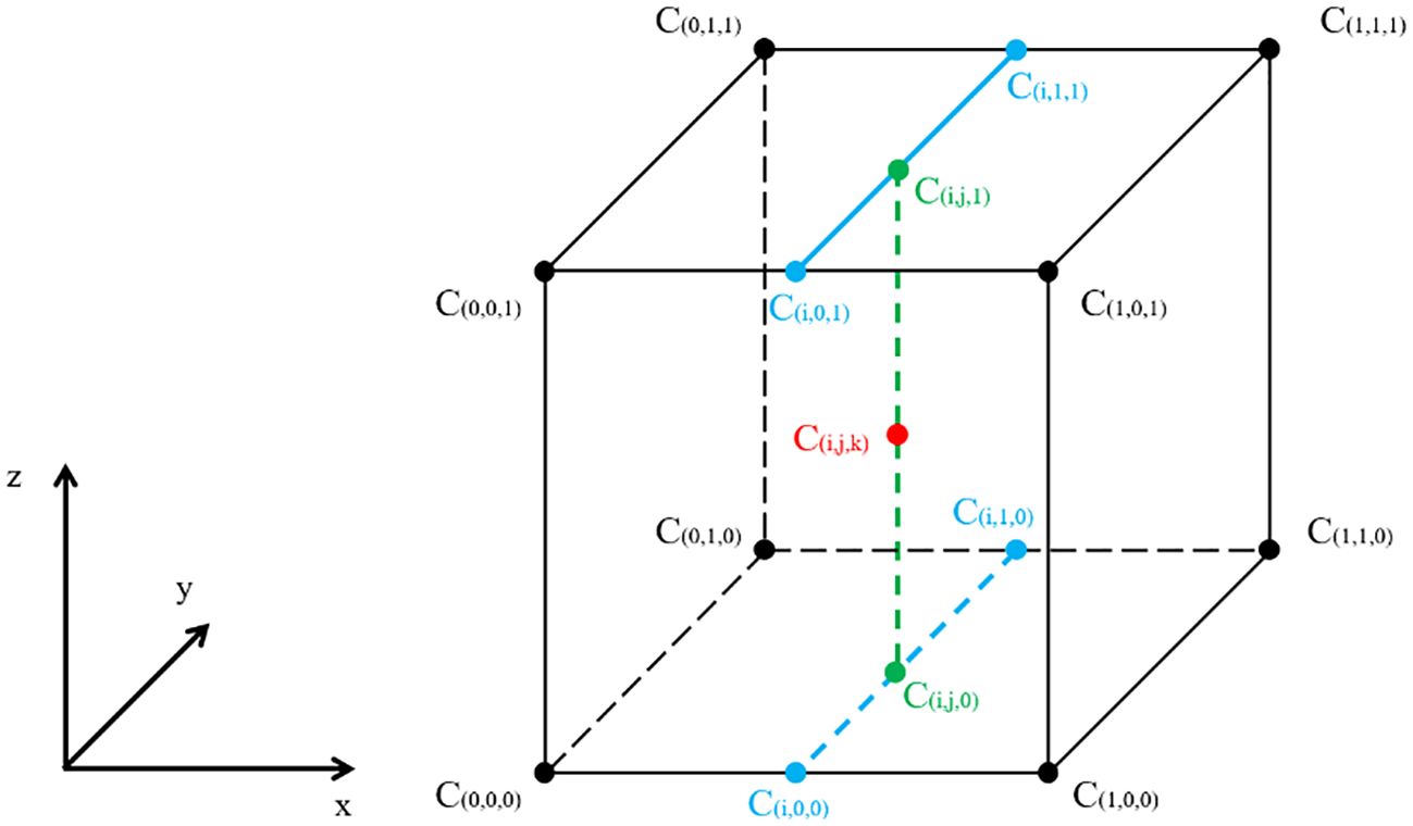
Figure 5 Trilinear Interpolation.

$\begin{array}{ll}\begin{array}{l}{C}_{(i,j,k)}=C_{(0,0,0)}(1-i)(1-j)(1-k)+C_{(1,0,0)}(1-j)(1-k)+C_{(0,1,0)}(1-i)j(1-k)+\\ C_{(1,1,0)}ij(1-k)+\\ C_{(0,0,1)}(1-i)(1-j)k+C_{(1,0,1)}i(1-j)k+\\ C_{(0,1,1)}(1-i)jk+C_{(1,1,1)}ijk\end{array}& (1)\end{array}$

In Equation 1, i, j, k∈[0, 1], are the fractional offsets of the sample positions in the x, y, and z directions. The results of trilinear interpolation are independent of the order of the interpolation steps along the three axes; any other order, e.g., along x, then y, and finally z, will yield the same values.

3) Integral synthesis of rays

In the preceding steps, color values for all the sampled points along the rays are acquired through texture resampling. These color values for all the rays are then combined to generate the final image (Hua, 2011). This process can be carried out for each pixel, and by sampling and averaging multiple pixels, the image’s quality and realism can be further enhanced.

Depending on the calculation direction, the synthesis process can be divided into two methods: front-to-back synthesis and back-to-front synthesis. In this study, the front-to-back synthesis method is employed (as depicted in Figure 6). This method facilitates the convenient assessment of cumulative opacity, allowing the algorithm to terminate prematurely when the cumulative opacity reaches 1. This acceleration technique improves the speed of volume rendering. The formula for color synthesis at each sampling point along a light ray is as follows:

Figure 6

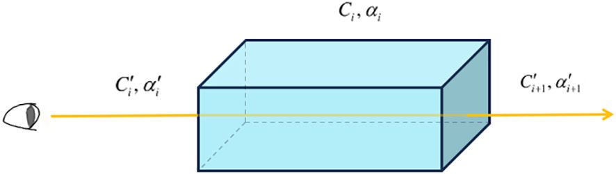
Figure 6 Integral synthesis of light from front to back.

$\begin{array}{ll}C={\displaystyle \sum _{i=1}^{\text{n}}{C}_i{\alpha }_i{\displaystyle \prod _{j=1}^{i=1}(1-{\alpha }_j)}}& (2)\end{array}$

where C is the final synthesized color, and C_i and α_i are the color and opacity of sampling point i along the light direction, respectively. From the Equation 2, the iterative formula for color synthesis from front to back can be derived:

$\begin{array}{ll}\{\begin{array}{c}{C}_{\text{i}+1}^{\text{'}}=C_i^{\text{'}}+(1-{\alpha }_i^{\text{'}})C_i{\alpha }_i\\ {\alpha }_{i+1}^{\text{'}}={\alpha }_i^{\text{'}}+(1-{\alpha }_i){\alpha }_i^{\text{'}}\end{array}& (3)\end{array}$

In Equation 3, $C_i^{\text{'}}$ is the color value accumulated from the 1st to the ith sampling point. ${\alpha }_i^{\text{'}}$ is the current cumulative opacity.

3.1.2 Sobel operator-based edge enhancement

In existing volume rendering visualizations, issues such as transparency iteration and color similarity often lead to blurring effects, especially when viewing the edge part of the rendered volume at tilted angles. This blurring diminishes the three-dimensional perception of the rendered volume, especially in scenes with colorful backgrounds like a 3D virtual Earth. It doesn’t contribute to enhancing the 3D visualization effect. To address this, this study introduces the Sobel operator to calculate the edge part of the volume rendering and enhance the edge colors to intensify the three-dimensional perception. The edge part of the volume rendering is where pixel colors exhibit significant variations. Edge detection aims to identify pixels with substantial changes and form a pixel point set to determine the target edge (Huanhuan et al., 2023). The Sobel operator is a commonly used technique for edge detection in two-dimensional (2D) images.

$\begin{array}{ll}X\text{ direction}:\left[\begin{array}{ccc}-1& 0& 1\\ -2& 0& 2\\ -1& 0& 1\end{array}\right] Y\text{ direction}:\left[\begin{array}{ccc}-1& -2& -1\\ 0& 0& 0\\ 1& 2& 1\end{array}\right]& (4)\end{array}$

As shown in Equation 4, the Sobel operator consists of two sets of 3x3 matrices. The values within these matrices represent the weighting factors for the corresponding pixels. Horizontal gradient values and vertical gradient values are obtained by convolving these matrices with the image in the horizontal and vertical directions, respectively (Chieh-Yang, 2016). Consider a point P (x, y) and its neighboring pixels in the image as shown in Equation 5:

$\begin{array}{ll}\left[\begin{array}{ccc}{P}_1& P_2& P_3\\ P_4& P(x,y)& P_6\\ P_7& P_8& P_9\end{array}\right]& (5)\end{array}$

Then the gradient values in the x and y directions can be obtained after plane convolution of P (x, y) with the matrices in both directions, as shown in Equation 6:

$\begin{array}{ll}{G}_{\text{x}}=\left[\begin{array}{ccc}-1& 0& 1\\ -2& 0& 2\\ -1& 0& 1\end{array}\right]*P(x,y) G_y=\left[\begin{array}{ccc}-1& -2& -1\\ 0& 0& 0\\ 1& 2& 1\end{array}\right]*P(x,y)& (6)\end{array}$

$\begin{array}{ll}G(x,y)=\sqrt{G{(x)}^2+G{(y)}^2}& (7)\end{array}$

The approximate gradient magnitude and gradient direction of pixel point P (x, y) can be calculated using Equation 7. If the value of G (x, y) is greater than a predefined threshold, then pixel point P (x, y) can be identified as an edge point. Subsequently, the color of the detected pixel point can be modified to make it stand out from the surrounding colors.

In the volume rendering process of this study, data is processed for rendering by reading it from the texture and retrieving the pixel colors from the texture, the specific process is shown in the Figure 7. After incorporating the edge enhancement method based on the Sobel operator, edge computations are performed on the texture before data processing. Since the data-free region in the texture lacks color, the pixels located at the edge of the data-free region can be computed, color-enhanced, and then rendered to the screen. This enhances the visibility and prominence of edges in the rendered volume.

Figure 7

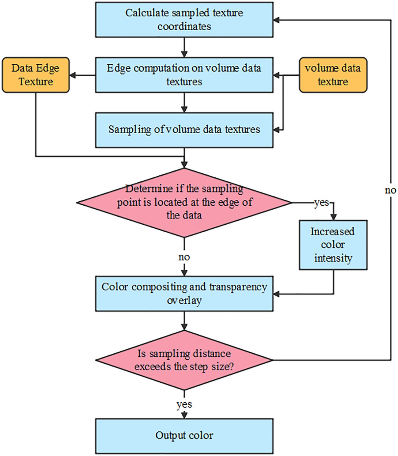
Figure 7 Flow of ray casting computation introducing edge detection.

3.1.3 Texture resampling hybrid interpolation

The traditional texture resampling method is to read the texture data of eight points around the point for each point of the light and then perform the tri-linear interpolation calculation, which requires 19 times of addition and subtraction and 24 times of multiplication to get the target value for each sampling, which greatly occupies the computational resources and reduces the drawing efficiency. Assuming that the light traverses n voxels and each voxel is sampled c times, with T₁ being the time required for the addition and subtraction operations and T₂ being the time required for the multiplication operations, the total resampling time T is shown in Equation 8:

$\begin{array}{ll}T=c\times n\times (19T_1+24T_2)& (8)\end{array}$

When c and n increase, the total time T also increases, and when T is too large, it is difficult to realize the effect of time-sequential dynamic volume rendering for a large range of volume data, which will lead to incomplete drawing effect, unsmooth dynamic effect and other problems, and it is necessary to reduce the computational complexity. The traditional texture resampling method is to sample the points inside the voxel with equal spacing, and this study proposes a resampling hybrid interpolation method to accelerate the sampling time, improve the drawing efficiency, and guarantee the effect of time-sequential dynamic drawing.

Figure 8, assuming that a ray of light (the blue line segment in the figure) traverses the voxel (the green cube in the Figure 8), with A as the point of incidence and B as the point of egress, c samples will be taken on the line segment AB, with the sample points i=1,2,3…c. Firstly, triple linear interpolation is performed on points A and B to obtain the values of V_A and V_B, and the incoming parameter s is received from outside to be used as the spacing of s to The sampling points on the line segment that satisfies i is a multiple of s (red points in the figure) are calculated by the trilinear interpolation method to obtain the values V_s,V_2s…,V_ns of these points, where n=1,2,3…. Afterward, a simple linear interpolation method is applied to the sampling points where i is not a multiple of s (yellow points in the figure) to compute the values. The overall Equation 9 is shown below:

Figure 8

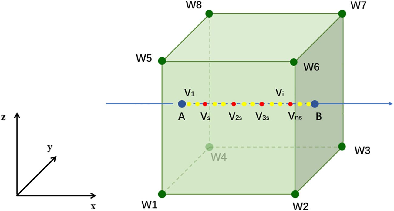
Figure 8 Resample hybrid interpolation.

$\begin{array}{ll}\{\begin{array}{l}{V}_{(i,j,k)}= W_1(1-i)(1-j)(1-k)+W_{2}i(1-j)(1-k)+W_3(1-i)j(1-k)+W_{4}ij(1-k)\\ +W_5(1-i)(1-j)k+W_{6}i(1-j)k+W_7(1-i)jk+W_{8}ijk, i\%s=0\\ V_i = V_{ns}+(V_{(n+1)s}-V_{ns})\times \frac{i-ns}{s}, i/s=n \& ns<i<(n+1)s\end{array}& (9)\end{array}$

A custom parameter s is used in Equation to be able to perform the trilinear interpolation computation with a larger spacing, after which a simple linear interpolation computation is performed for the remaining points, in particular, when i is smaller than s, the computation of linear interpolation is performed using V_A with V_s, and when (n+1)s is larger than c, the computation of linear interpolation is performed using V_ns with V_B. Let the light traverses n voxels and each voxel is sampled c times, T₁ is the time required for addition and subtraction operations and T₂ is the time required for multiplication operations, then the total resampling time T of the algorithm proposed in this study is shown in Equation 10:

$\begin{array}{ll}T=c\times n\times [\frac{1}{s}\times (15T_1+18T_2)+(4T_1+6T_2)]& (10)\end{array}$

Assuming that the number of samples c=30, the number of voxels n=100, and the customization spacing s=3, the sampling time T=57000T₁ + 72000T₂ obtained from the formula of the traditional trilinear interpolation method, and the sampling time T=27000T₁ + 36000T₂ of the hybrid interpolation method proposed in this study, it can be seen that the computational complexity in this study is low, and it can achieve the plotting effect and the efficiency of the plotting balance of the plotting effect and plotting efficiency.

3.2 Dynamic visualization of particle systems based on Lagrangian fields

3.2.1 Algorithms and architectures for particle systems

Particle system is a commonly used technology in computer graphics for simulating and presenting the movement of massive tiny particles, particle system is based on the concept of particles, each particle is a virtual point or object with some attributes, such as position, speed, color, life span and so on (Thomas and John, 2010). These attributes can be changed over time to simulating the movement and performance of particles in the scene. The spatial distribution of a large number of particles in the particle system can reflect the intensive degree of the phenomenon and the regular movement of a large number of particles can reflect the change rule and change trend of the phenomenon (Wenjun, 2017).

The particle system algorithm of this study is shown in Figure 9, which can be divided into the stages of data parsing, initial parameter acquisition, particle life cycle control, particle dynamic tracking and rendering.

(1) Data resolution stage: this study uses the typhoon wind field data in NetCDF format as the data source of the particle system, and because the raw data has the characteristics of multi-layer and large time resolution, its processing includes data dimensionality reduction, time interpolation and other steps. Finally, color space mapping is performed on the data, and the U-direction values and V-direction values in the wind field data information stored in the grid dataset are converted to the corresponding RGB color values, which are then stored into the picture to form the data texture, so as to perform high-speed reading and data deciphering in the particle system to obtain the original data values.

(2) Initial Parameter Acquisition Stage: This stage receives incoming customized particle parameters from the outside, including the number of particles, particle speed multiplier, particle lifetime, particle width, etc. These parameters determine the final particle system rendered into the scene particle density, the total length of the particle traveling line and other rendering effects.

(3) Particle life cycle control phase: after obtaining the particle life in the initial parameters, randomly lay down the initial particles, drive the particles to move, judge the life state of the particles every time they move, delete the particles that meet the conditions of extinction and create new particles at a random location within the data area, and cycle the algorithm to ensure that the density of particles in the scene is uniform.

(4) Particle Dynamic Tracking and Rendering Stage: This stage is responsible for updating the position of particles and rendering them to the scene. During the particle movement, the next moment position and velocity of the particle are constantly calculated to drive the next frame of the movement of the particle, and the corresponding color and step size are calculated according to the particle velocity.

Figure 9

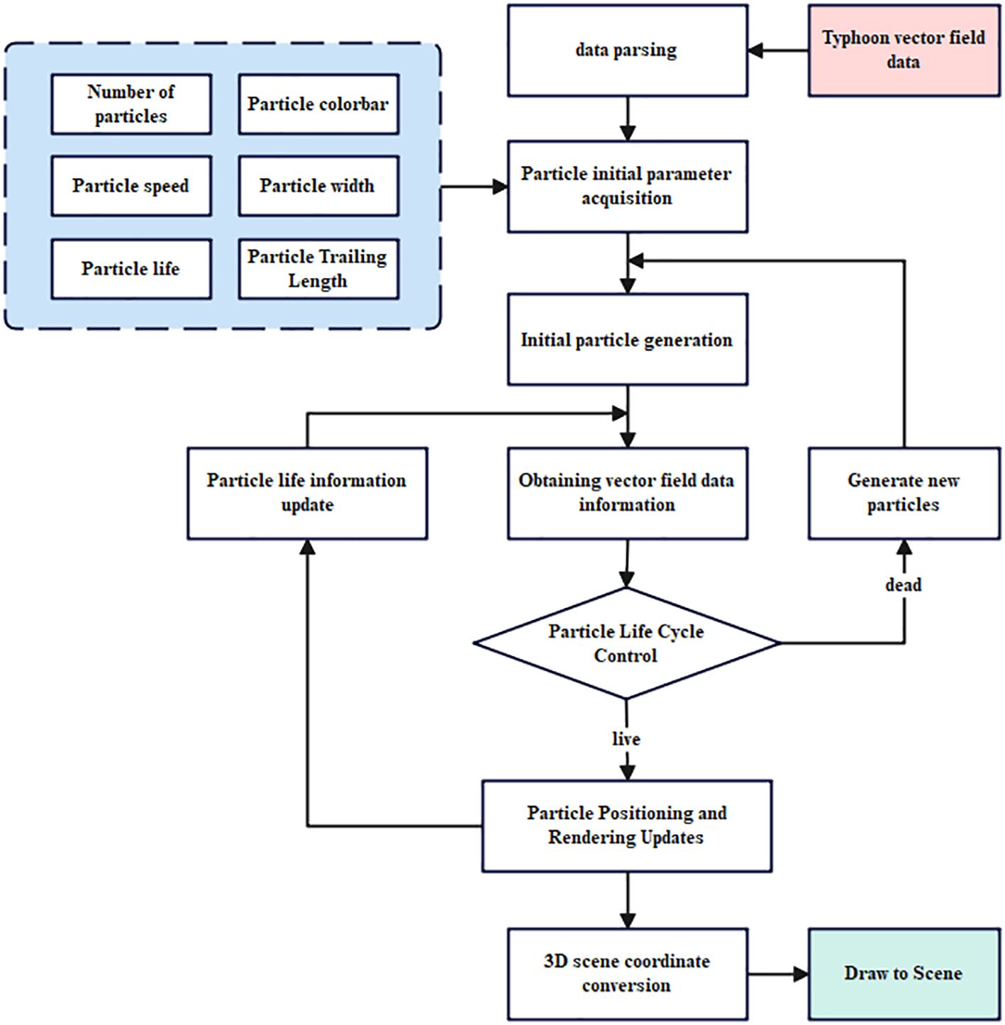
Figure 9 Particle System Algorithm Flow.

This study implements a particle system based on WebGL technology, and the work in GPU is mainly divided into particle parallel tracking computation and particle dynamic rendering, the architecture of the particle system based on WebGL is shown in Figure 10.

Figure 10

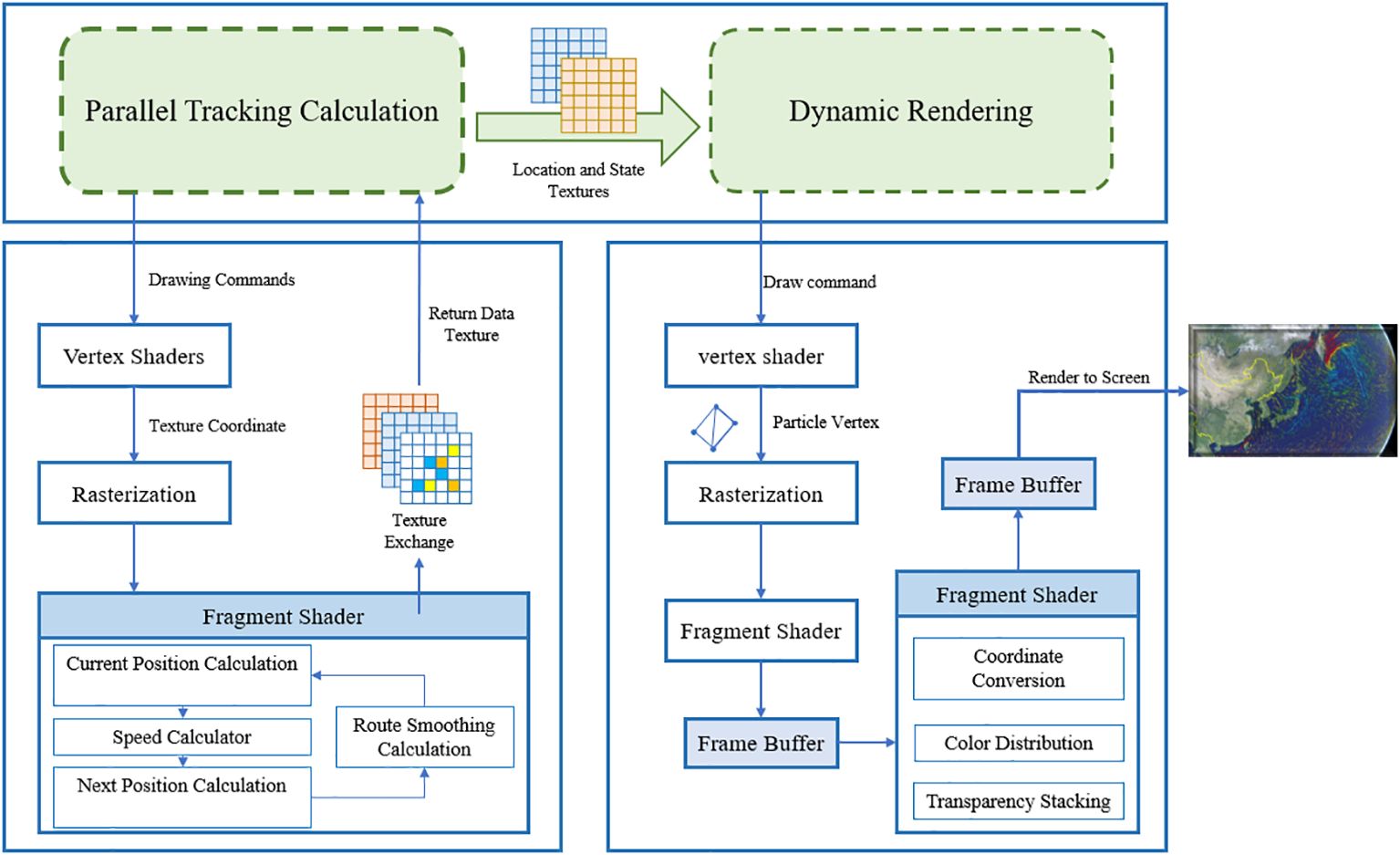
Figure 10 Particle system architecture.

The parallel tracking computation part processes the vertices to get the rasterized data, by creating four textures and constantly exchanging the texture of the next moment, it completes the parallel computation of the position and motion of a large number of particles. Then, it exchanges textures with the previous moment to realize real-time update of the data state, and then passed into the particle dynamic rendering process, which realizes the symbolization and dynamic rendering of particles by creating the head of particles, calculating the tail of particles, and iterating the opacity of the tail of particles. In terms of parallel computing, this study considers the motion calculation of each particle as a separate task, and the processing of texture in GPU is executed in parallel, with no influence between particles, thus realizing the simultaneous calculation and driving of massive particles.

3.2.2 Parallel tracking of particles

After receiving the draw command, the vertex shader outputs the coordinates of the processed data texture vertices and enters the rasterization stage to process the vertices into pixels. This study writes the kernel function in the piecewise shader, and by calculating and replacing the four textures, the mass particle parallel tracking computation task is divided into four subtasks, namely, current position calculation, velocity calculation, next moment position calculation, and state management calculation, and cycle executes the subtasks to compute the motion of the mass particles. The specific steps are shown in Figure 11.

(1) Create a particle current position texture, randomly generate initial particles in the texture and record the coordinates of the particles. Create velocity texture, next moment position texture and particle state texture, pass them into the slice shader together with the typhoon vector field data texture.

(2) Calculate the current velocity texture of the particle. The current position texture of the particle coincides with the incoming wind field data texture, then each particle can read the U and V values of the wind field on the corresponding pixels in the wind field texture, and calculate to get the velocity of the motion, which is stored into the velocity texture.

(3) Calculate next moment position texture. After obtaining the current position and velocity of the particle, we can calculate the new position that the particle will move to in the next moment, store it in the next moment texture, and exchange the next moment texture to the current position texture, change the coordinate of the particle to the new position, and then return to (2) to calculate the velocity, and so on will realize the continuous movement of the particle.

(4) Performs life state management of particles. Judge the life state of the particle before the velocity calculation, if the particle reaches the extinction condition, then remove the particle, and at the same time generate a new initial particle in the data area to participate in the velocity calculation. If the particle moves to the empty data area and exceeds the boundary of the data area, it will also be removed.

Figure 11

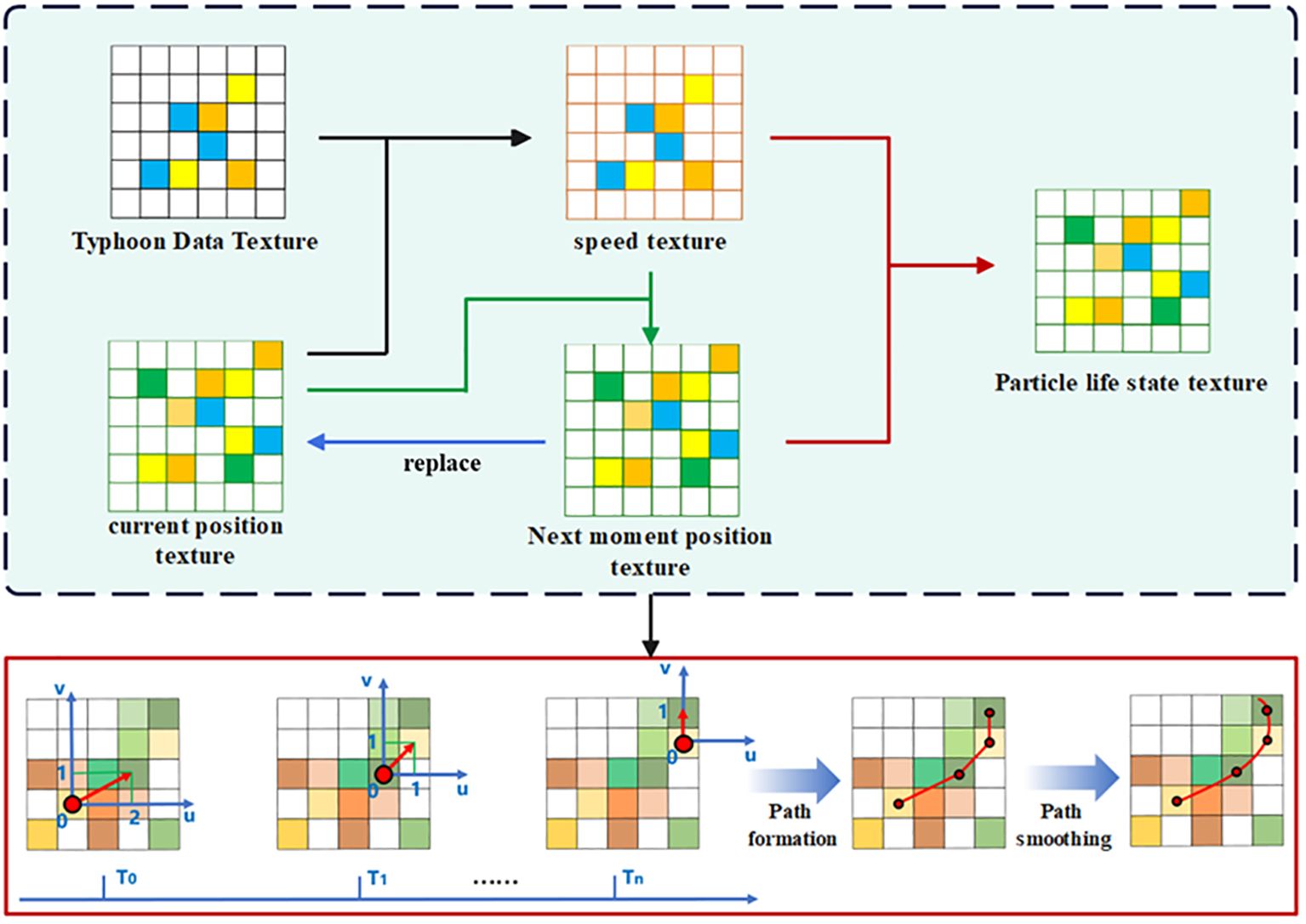
Figure 11 Particle Parallel Tracking Process.

In the process of particle movement, if the linear movement is carried out strictly by the position of the next moment derived from the calculation, there will be a huge number of particles with folded trajectories, which reduces the visualization effect of the particle system. To solve this problem, this study, after comprehensively comparing the effect and computational speed of path smoothing algorithms such as spline curve, least squares method and Bessel curve, Bessel curve is chosen to generate smooth paths through the control points, which has a simple computation and high quality of smoothing, and the computational formulas are shown in Equation 11.

$\begin{array}{ll}\begin{array}{l} p(t)={\displaystyle \sum _{i=0}^n{P}_i{B}_{i,n}(t) \mathrm{0\le t\le 1}}\\ B_{i,n}(t)=C_n^{i}i(1-t{)}^{n-i},C_n^i=\frac{\mathrm{n!}}{\mathrm{i!}(n-i)!} (i=0,1,\dots \dots ,n)\end{array}& (11)\end{array}$

3.2.3 Dynamic rendering of particles

After obtaining the motion path of each particle by parallel tracking calculation, if it is directly rendered to the screen, only a series of colorless motion points can be obtained, which can’t reflect the mobility of the typhoon well, so it is necessary to symbolize the motion points, generate the head and tail of particles, and match the transparency change with the color band to realize the visualization of the wind field of the typhoon. In this study, we use the texture obtained from the parallel tracking calculation to create the particle dynamic rendering task, which is divided into four sub-tasks: particle head creation, particle tail creation, particle tail transparency calculation, and particle color calculation, and the specific steps are shown in Figure 12.

(1) Particle head creation: Get the two positions of the particle in the current position texture and the next moment position texture, connect them and make a vertical line through these two points, and get two points on the vertical line as the offset points of the original points, so as to create two triangles, and then splice them together to form a rectangle particle head, as shown in Figure 12(1). Finally, the particle head is created and stored in the head texture.

(2) Particle trailing creation: after getting the head texture from the previous step, create an empty trailing texture for each particle. When the particle moves to the next moment, the position of the particle head in the head texture is updated, but before updating, the original position of the head is copied to the particle tail texture, and the process is looped to get a series of tail rectangles until the particle dies or reaches the maximum length of the particle’s tail, as shown in Figure 12(2).

(3) Particle Tail Transparency Calculation: After obtaining the particle tail texture obtained in the previous step, the transparency of the trailing rectangle stored in the particle tail texture will be increased by a certain percentage after each unit of time, and the trailing rectangle will be cleared when the transparency is zero to form a trailing effect that will fade away, as shown in Figure 12(3).

(4) Particle color calculation: according to the current speed of the particle, get the corresponding color in the ribbon and assign it to the head texture, so that the particle can react to the speed of movement by the color.

Figure 12

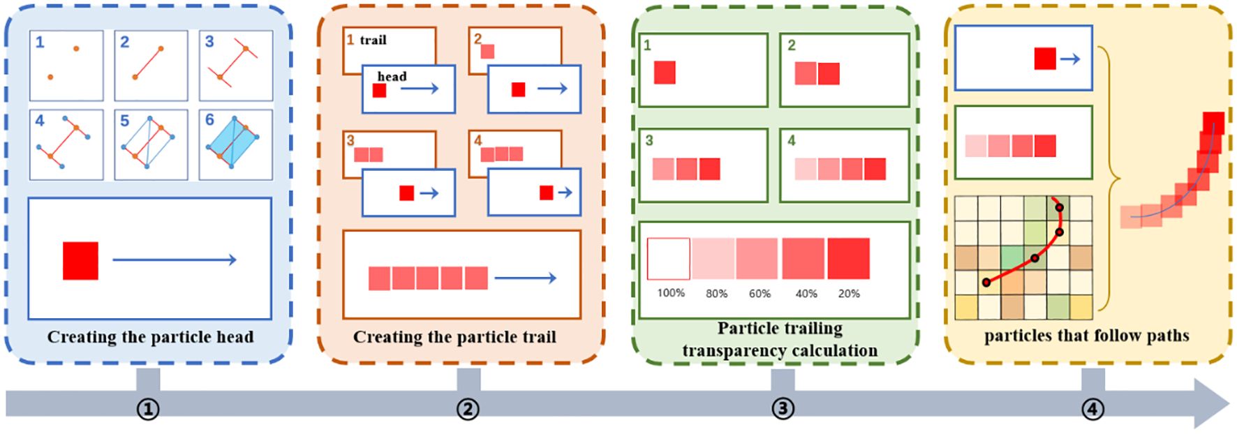
Figure 12 Particle dynamic rendering steps.

Finally, the particle head texture is combined with the trailing texture to move according to the path obtained by parallel tracking, as shown in Figure 12(4), which can realize the dynamic rendering of a large number of particles.

3.2.4 Calculation of particle trajectories based on Lagrangian fields

Most of the current studies of particle systems are Euler field particle systems, which can only show the instantaneous vector field and cannot simulate the time-series dynamic motion of the vector field, which needs to be tracked and computed for the long time-series motion of the particles. There are two main particle tracking methods, Lagrangian and Eulerian, and this study is based on the Lagrangian method, which introduces the Lagrangian field that describes the motion of nonlinear particles into the visualization of typhoons to mine the characteristics of typhoon changes in consecutive moments.

Lagrangian fields have their origins in the theory of dynamical systems and are used to describe the variation of fluids in nonlinear dynamical systems using unsteady fields to study the variation of particles in space over time. Considering each particle in the particle system as a mass point, the particle can be tracked continuously over time to obtain its position at different moments and thus form a trace, which realizes the effect of continuous dynamic visualization of a large number of particles.

Trace is the method of describing the flow with Lagrangian method, it is the same particle in space when the motion of the curve depicted, can also be understood as the particle at different moments in the location of the formation of the curve, as shown in the Figure 13. In the particle system of this study, firstly, the data texture of consecutive moments is looped into the particle system to obtain the data of consecutive moments, and the array of positions of the particles over time is calculated, so as to compute the trajectory of each particle, which is carried out in the following steps:

(1) Generate particles randomly and obtain the initial coordinates of the particles.

(2) In the parallel tracking part of the particle system, calculate the current position and the next moment position of the particle with the data of T₀ moment, store it into the texture, and hand it over to the dynamic rendering part to realize the movement of the particle.

(3) Pass the data of T₁ moment into the parallel tracking part, calculate the next moment position of the data of T₁ moment, and store it into the texture to realize the movement of the particle in the new moment.

Figure 13

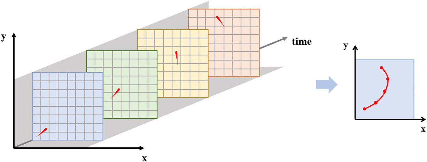
Figure 13 Formation of trace lines.

Repeat the execution of step (3) to calculate the motion direction and position of the current particle at each moment, and integrate to derive the trajectory of the particle. The Lagrangian field expression of the particle system can be realized by tracking the trajectory of each particle in parallel.

3.3 Frame buffer-based hybrid drawing method

In this study, a typhoon is drawn on a 2D canvas using WebGL and then visualized on a 3D sphere through coordinate transformation. When simply superimposing the scalar and vector fields, a problem arises: incorrect occlusion between the graphics, causing all the particles to appear above the volume data. As shown in Figure 14, the left side of the figure demonstrates the occlusion issue between the two layers of scalar and vector fields, while the right side illustrates the actual drawing process, revealing that particles from all layers are rendered above the volume rendering effect. This results in a failure to merge the scalar and vector fields, negatively impacting the visualization effect.

Figure 14

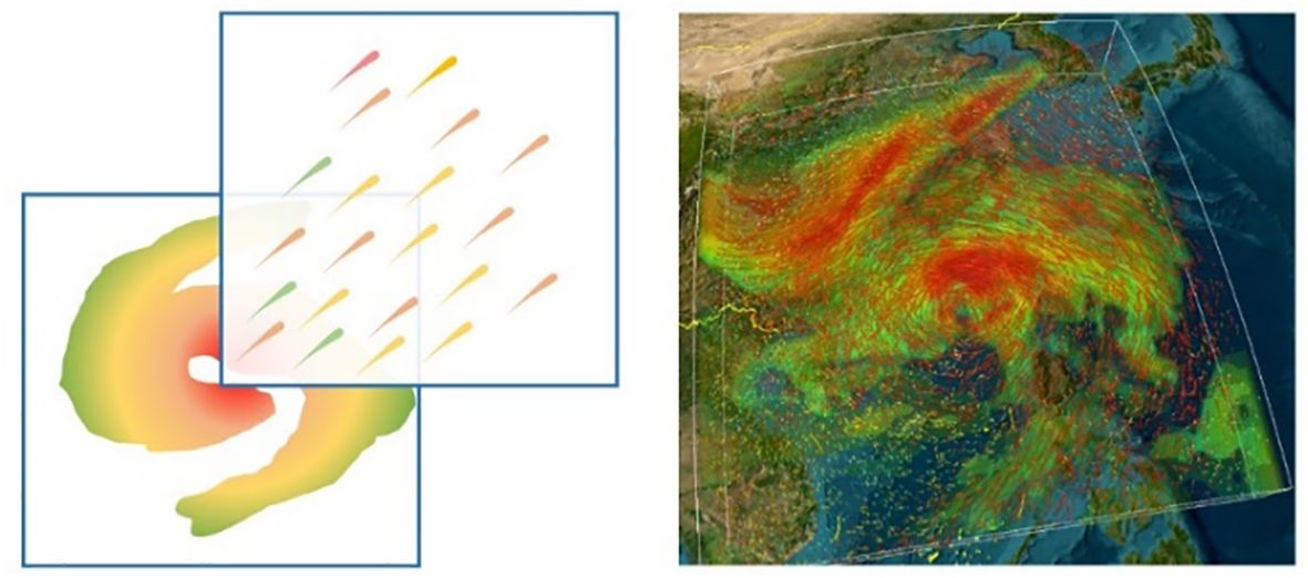
Figure 14 Graphic masking schematic.

To address this issue, this study proposes a fusion drawing method that uses depth values to determine the occlusion relationship between the scalar and vector fields. By calculating the blending color, this method ensures that the final image displayed on the screen maintains the correct occlusion relationship, achieving the fusion of the scalar and vector fields. The fundamental concept of this method is to render the particles in the vector field twice during the rendering of the scalar and vector fields. In the first rendering pass, depth and color information of the particles is drawn into the depth buffer and color buffer of the frame buffer object. In the second rendering pass, particles and the scalar field volume model are drawn based on the depth and color information generated in the previous step. The Z-Buffer algorithm is utilized to achieve depth-based fusion of volume rendering and particles, ensuring the correct occlusion relationship.

In the rendering pipeline of WebGL, data and textures are ultimately transformed into two-dimensional pixels that will be displayed on the screen. The frame buffer is a crucial component in this process, serving as the final stage before actual rendering. It contains pixel-related information about the image to be rendered. The frame buffer encompasses various buffers, including a depth buffer, a color buffer, and a stencil buffer, which collectively enable post-processing of the image before it’s displayed on the screen. Frame buffer objects provide a means to render to a texture that can be subsequently used as input for the next shader (Jiani, 2013). They are often a more straightforward and efficient choice compared to other similar techniques for rendering and post-processing in WebGL.

The Z-Buffer algorithm used in the hybrid drawing method of this study operates at the pixel level, which helps avoid problems related to complex occlusions. As depicted in Supplementary Figure 2, the algorithm begins by allocating an array called the “Buffer”, where the size of the array corresponds to the number of pixels. Each element in the array represents the depth and starts with an initial depth value of infinity (Siting, 2017). The algorithm then proceeds to traverse each pixel point [x, y] on each object. If the depth value “z” of that pixel point is less than the value in Buffer [x, y], the Buffer [x, y] value is updated with the depth value “z” of that point, and the color of the pixel point [x, y] is also updated.

The hybrid volume drawing method in this study is based on direct volume rendering and requires special blending based on cached depth information during color blending. In traditional ray casting, which is a direct volume rendering algorithm, there is no depth test with alpha blending during the color mixing and accumulation process. The drawing process in this study utilizes a frame buffer object and the Z-Buffer algorithm. When determining the drawing color of screen points, a ray is emitted from the observation point into the scene, and the following cases are considered:

1) When the ray does not intersect with the volume model and the particles, the screen color is the background color.

2) When the ray only intersects with the volume model, the traditional ray casting algorithm is used.

3) When the ray only intersects with the particles, the particle system is drawn.

4) When the ray intersects with the volume data and the particles, the hybrid volume drawing method is employed.

The specific steps for the hybrid volume drawing method are as follows:

1) Store the information of particles in the frame buffer object (FBO), where the color value is saved in the color buffer, and the depth value is saved in the depth buffer.

2) Calculate the sampling ray R, the sampling start point P₁, and the sampling end point Pn.

3) Retrieve the color value C and depth value D from the FBO.

4) Cyclically sample the texture and synthesize colors while using the Z-Buffer algorithm to compare the depth values D_i and D for each sampling point i. If i< n and D_i< D, it means the volume data at the current point is closer to the observation point than the particles. In this case, the colors are blended based on the volume data value, and the corresponding colors are searched for in the color table. Sampling proceeds to the next point. If i< n and D_i > D, it means the particles at the current point are closer to the observation point than the volume data. The color C from the FBO is used as the color of the current point, and since the particle blocks the volume data on the ray R located after the point, no further sampling is performed, and the loop is skipped. When i = n, the loop is also skipped.

5) Mix the color values obtained from sampling and finally output the final color of the point on the screen as shown in Equation 12:

$\begin{array}{ll}{C}_{\text{f}}=C_s+[1.0-C_s·\alpha \times (1.0-\lambda )]\times C& (12)\end{array}$

Where, $C_f$ is the final color of the pixel in the screen, $C_s$ is the cumulative color of the light passing through the volume data, $\alpha$ is the cumulative opacity, $\lambda$ is the adjustment parameter for the opacity, and $C$ is the color value of the point stored in the FBO. If the ray passes through only the particle, $C_s$ has no value and the final color is the particle color; if the ray passes through only the volume data, $C$ has no value and the final color is the cumulative color of the volume data; if the ray passes through the volume data and the particle, the final color is calculated by $C_s$ and $C$ together.

4 Result and discussions

In this study, based on the research proposal in the previous section, a series of experiments are designed to evaluate the effectiveness and efficiency of the dynamic visualization of the integration of vector and scalar fields for typhoons.

4.1 Dataset and processing

4.1.1 Dataset

In this study, Super Typhoon Hato is chosen as the subject for typhoon visualization. Super Typhoon Hato was first identified to have developed at 14:00 on August 20, 2017, in the Northwest Pacific Ocean. Its intensity continuously increased, reaching the highest level, 15. It was officially recognized as a powerful typhoon and made landfall in Zhuhai City, Guangdong Province, China, around 12:50 p.m. on the 23rd. The data used for this study comprise various meteorological parameters, including cloud cover, wind speed, wind direction, air temperature, and air pressure. Since Super Typhoon Hato has a high hazard level, a wide range of influence, and a large movement, which has caused serious economic and social losses, and is representative, for the purposes of this study, we specifically focus on wind speed and wind direction data, which are utilized to visualize the scalar and vector fields, respectively.

The experimental data utilized in this study are derived from ERA5 reanalysis data produced by the European Centre for Medium-Range Weather Forecasts (ECMWF). The raw data is provided in GRIB format and includes wind speed and wind direction data, with the latter being split into u-direction and v-direction components. To adapt this data for our study, we conducted file format conversion and spatial cropping, resulting in NetCDF formatted data tailored to our specific region of interest. Detailed information about the dataset can be found in Table 1.

Table 1

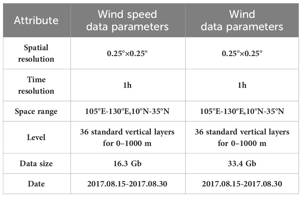
Table 1 Summary of the experimental datasets.

4.1.2 Data processing

Before undertaking the actual process of dynamic typhoon visualization, the initial dataset must be organized and transformed into corresponding texture images. Data preprocessing involves several essential steps, including data dimensionality reduction, time interpolation, and color space mapping. The specific procedures are illustrated in Supplementary Figure 4.

(1) Data dimensionality reduction: Typhoon volume data cannot be directly used in volume rendering algorithms and particle systems, so it’s necessary to reduce the data’s dimensionality (Ayesha et al., 2020). First, the multidimensional typhoon volume data are downscaled along the time dimension, breaking down the original data into 3D volume data with the same spatial range based on temporal resolution. Subsequently, these acquired 3D volume data are further downscaled according to the data’s height hierarchy, transforming them into 2D mesh data with the same horizontal range. Finally, the resulting 2D mesh data is organized into a 2D mesh dataset.

(2) Temporal interpolation: The 2D grid data has time intervals, and if dynamic visualization is performed directly according to the time sequence, the rendering frame rate may not meet the requirements for smooth frame animation. This can result in a lagging screen and a failure to achieve the desired coherent simulation of typhoon movement. To achieve a smoother animation effect, temporal interpolation is necessary (Li and Revesz, 2004). It involves interpolating the time series data along the time axis to obtain data between two observation time points and rendering them in real time. This approach enables a smooth transition between two key frames (Xuequan, 2020). In this study, a simple linear interpolation calculation is employed to resample data between frames in the time series. Assuming that a certain data in the grid data D_n at one moment is represented as V_n, and the data in the grid data Dn+1 at the next moment is Vn+1, the data V_x at a specific time between these two frames is calculated as shown in Equation 13:

$\begin{array}{ll}{V}_x=V_n+(V_{n+1}-V_n)\ast \frac{T_x-T_n}{T_{x+1}-T_n}& (13)\end{array}$

(3) Color space mapping: Following data dimensionality reduction and temporal interpolation, the data must undergo color space mapping to transform the discrete voxel information stored in the grid dataset into a coherent texture for storage (Lei et al., 2022). In the GLSL rendering process employed in this study, images are used as a data format, as they can be quickly read. Therefore, images serve as the medium for volume texture storage. Initially, an empty image with the same resolution as the 2D grid data is created. Subsequently, the data stored at each grid point is deposited into the RGB color channel of the corresponding pixel in the image.

4.2 Experiments on typhoon visualization effects

This study validates the effectiveness of the integration of vector and scalar fields for dynamic visualization using reanalysis data from Super Typhoon Hato. The data covers a height range from 1 meter to 1000 meters, which is relatively flat compared to the latitude and longitude range of the data, approximating surface mapping. To enhance the stereoscopic effect of the volume rendering and the 3D particle system, the height range of the data volume is exaggerated.

The volume rendered visualization is depicted in Supplementary Figure 5, where the colors ranging from red to blue represent wind speed from high to low. Supplementary Figure 5A displays the visualization from a top view, while Supplementary Figures 5B, C present the visualization from two side views. These images clearly depict characteristic information and internal details of the typhoon, including the eye of the typhoon and the outer strong wind zone. Additionally, the three-dimensional visualization showcases the variation in wind speed at different altitude levels and the three-dimensional structure of the vortex. Moreover, this study provides customized sectioning effects along the x, y, and z axes in the rendering, as shown in Supplementary Figure 5D for the x-axis, Supplementary Figure 5E for the y-axis, and Supplementary Figure 5F for the z-axis in Supplementary Figure 5, facilitating the study of internal changes within the typhoon.

The particle system visualization effect is presented in Supplementary Figure 6, where the colors range from red to blue to represent wind speed from high to low. Supplementary Figure 6A displays the visualization effect from a top view, while Supplementary Figures 6B, C showcase the visualization effect from two side view perspectives. In this figure, it’s evident that the particle system-based typhoon visualization method effectively conveys wind direction and wind speed at different altitude levels within the typhoon. This approach provides a more intuitive representation of the spatial characteristics of the typhoon’s eye region. Additionally, this study incorporates the Lagrangian field concept within the particle system, enabling the particles to continuously update their motion speed and direction at any given time sequence, resulting in a dynamic particle tracking effect. This feature allows for the visualization of the typhoon’s motion trajectory over time and the characteristic changes in its movement, as demonstrated in Supplementary Figure 6A.

The dynamic visualization of the integration of vector and scalar fields for the typhoon is presented in Supplementary Figures 7A–C showcase the visualization effects from a top view and two side view perspectives, respectively. This approach combines volume rendering to accurately depict the morphology and internal details of the typhoon with a particle system to convey the detailed flow of the typhoon, resulting in a three-dimensional dynamic visualization that enhances the sense of realism.

Furthermore, Supplementary Figure 7D demonstrates the time-series visualization, where clicking the play button opens the dynamic time-series visualization of the data. This visualization effectively illustrates the entire lifecycle of Super Typhoon Hato, including its generation, movement, typhoon eye formation, landfall situation, and the smooth change of peripheral wind bands. It allows for the analysis of specific characteristics of the typhoon, including:

1) Small Typhoon Radius: The visualization shows that Super Typhoon Hato had a relatively small wind radius of about 40 to 50 km. This made it challenging to assess its intensity based solely on its size. The high winds brought by the typhoon only became evident shortly before landfall, and ground-based meteorological stations couldn’t observe them earlier.

2) Dramatic Path Changes: The time-series visualization reveals that Super Typhoon Hato initially approached the eastern part of Guangdong Province, China, on August 21, 2017, but then shifted its path to the Pearl River Estuary on August 22, 2017. Its movement speed increased in the South China Sea, which posed significant challenges for defense and navigation (Luo et al., 2020).

3) Intensity Variations: The intensity of the typhoon underwent dramatic changes. While forecasts initially predicted a tropical storm, the typhoon’s winds surged significantly in a short period. It rapidly escalated from a Category 1 typhoon to a Category 5 super typhoon in less than a day, catching forecasters off guard.

4) Unfavorable Path: Super Typhoon Hato’s path brought it to the right side of the densely populated Pearl River Delta (PRD) city clusters in southern China. This positioning resulted in severe damage to cities like Guangzhou, Shenzhen, Zhuhai, and Foshan, all located in the PRD region.

Regarding the fusion experiment of vector and scalar fields, the effect is depicted in Supplementary Figure 8A illustrates the effect without the fusion of scalar and vector fields. In this scenario, the vector field appears to float above the volume rendering effect, resulting in incorrect occlusion between data layers. Additionally, the particles in the typhoon’s eye region appear above the volume rendering. Supplementary Figure 8B demonstrates the effect of the fusion plotting of scalar and vector fields, which rectifies the shading relationship between the two, and particles in the typhoon’s eye region interact dynamically with the volume model. The fusion plotting method used in this study effectively addresses these issues.

4.3 Typhoon visualization efficiency experiments

To validate the overall rendering performance of the proposed method in this study, rendering efficiency experiments are designed to evaluate the performance of the proposed method in this paper, using the average frame rate in a 3D scene as an evaluation criterion for efficiency. Performance test machine performance is: CPU model AMD Ryzen 9 5900HX with Radeon Graphics (3.00GHz), GPU model NVIDIA GeForce RTX 3060 Laptop, and the size of the running memory is 32GB.

During the time-sequence rendering process of the volume rendering method and the particle system rendering method, the change of the data volume at different moments and the selection of the rendering method will affect the rendering frame rate. In this study, the average change of the frame rate of the Super Typhoon Hato time-sequence dynamic visualization is recorded by fixing the height of the viewpoints, and the time period of the largest data change is selected as shown in Supplementary Figure 9.

As can be seen from the figure, the average frame rate of the three visualizations fluctuates over time as the data changes, but is not lower than 44.7. In human visual perception, a smoothing effect can be achieved when the frame rate is greater than 24, so this study’s dynamic visualization method for Super Typhoon Hato data can maintain a smooth visual effect.

Meanwhile, to test the plotting efficiency of the texture resampling hybrid interpolation method proposed in this study, the traditional trilinear interpolation sampling algorithm is set up as a comparative experiment, and the average frame rate is tested for the consecutive moments of Super Typhoon Hato’s landfall in the South China Sea, and the customized spacing s of the hybrid interpolation method is set to be 3.

Supplementary Figure 10, the typhoon has just traveled to the South China Sea at the moments of t0 and t1, and at this time, the amount of data is less, and the hybrid interpolation sampling method is slightly better than the traditional sampling method in the frame rate test. At moments t2 to t4, the typhoon travels and makes landfall in the South China Sea, and the data volume is large, this study’s hybrid interpolation sampling method shows high efficiency by improving the frame rate by an average of 21.9% compared with the traditional sampling method. At moments t5 to t7, the typhoon gradually weakens after making landfall, the data volume decreases, and the gap between the two algorithms decreases.

4.4 Verification of accuracy and generalizability

To verify the accuracy of the visualization effect of this study, we obtain the satellite images of Super Typhoon Hato’s real cloud amount in chronological order, and make a comparison with the temporal dynamic visualization effect of this study, and the effect is shown in the Supplementary Figure 11.

It is concluded that the range of typhoon in this study is consistent with that in the satellite cloud map, and the motion path and rotation direction of the typhoon shown in the cloud map are consistent with the motion of the visualized wind effect in this study. In addition, the detailed features such as the location and morphology of the typhoon eye and the morphology of the peripheral wind band shown in the visualization effect of this study are similar to the detailed features of the cloud shown in the cloud diagram. It can be seen that the visualization effect in this study has good accuracy and can simulate the motion pattern of the real typhoon.

In addition, to verify the generality of the visualization method in this study, another typhoon Pakhar is selected as the visualization object, the data of this typhoon include wind speed and direction with a resolution of 0.25x0.25 and a time resolution of 1h. The effect is shown in the Supplementary Figure 12.

Supplementary Figure 12, Typhoon Pakhar was located in the South China Sea on August 27, 2017, and the visualization effect of Typhoon Pakhar in this study is shown in Supplementary Figure 12C, which is able to clearly observe the direction of the typhoon, the change of the wind and the change of the typhoon’s shape. Moreover, the distribution of clouds in the satellite cloud map of Typhoon Pakhar matches the visualization effect of this study. It can be seen that the visualization method in this study has good versatility and is capable of visualizing other typhoons.

5 Conclusion

Most of the existing volume rendering schemes are single-moment and static expressions, and they are weak in expressing the structural characteristics and wind direction of typhoons. And although the particle system is widely used to express the wind field as a kind of meteorological data, the method is mostly a two-dimensional expression effect, which is not suitable for the three-dimensional expression of the typhoon at multiple levels. To enhance the three-dimensional dynamic visualization of typhoon, clearly show the structural change and moving trend of typhoon, and make up for the respective disadvantages of volume rendering and particle system, this study focuses on the integration of vector and scalar fields expression to improve the visualization effect and efficiency of typhoon based on the existing research scheme, and the main contributions are as follows:

Based on the ray casting method to realize the visualization effect of volume rendering for typhoon scalar data, the hybrid interpolation method during ray resampling is proposed to improve the computational efficiency of volume rendering, which shows high efficiency with an average increase of 21.9% in the frame rate compared to the traditional sampling method. Meanwhile, the Sobel operator is introduced to enhance the clarity of data edges and improve the comprehensive visualization effect.

A WebGL-based particle system is implemented for the visualization of typhoon vector data. The process of calculating the motion of multi-layer massive particles is divided into two parts: parallel tracking and dynamic rendering, which improves the computational efficiency, and the trajectory calculation of the Lagrangian field is introduced, which realizes the time-series dynamic visualization of the three-dimensional particle system.

The fusion representation of the typhoon vector field and scalar field is realized based on the frame caching technique. The depth texture of the particles is generated, the intersection of the particle and volume data of each ray in the ray casting method is judged, and the blended color accumulated by the ray is calculated based on the judgment result, and the correct shading relationship between the vector field and the scalar field is obtained. Based on the above method, the Lagrangian field expression of the wind speed and direction of the typhoon is realized, which can reflect the evolution of the typhoon and its travel route, and the rendering frame rate is greater than 44, which can achieve a stable and smooth rendering effect.

However, the study area of this study is limited to the vicinity of the South China Sea, and it needs to be expanded to realize the large-scale dynamic visualization of the typhoon vector scale as a whole. Meanwhile, the vertical velocity of the wind field should be added to the 3D particle system to obtain a better three-dimensional effect. In addition, it should be optimized for the lateral layering phenomenon of volume rendering effects, which is a future research direction.

Data availability statement

Publicly available datasets were analyzed in this study. This data can be found here: https://www.ecmwf.int/en/forecasts/datasets.

Author contributions

CF: Data curation, Formal analysis, Methodology, Software, Validation, Visualization, Writing – original draft, Writing – review & editing, Investigation. TQ: Data curation, Formal analysis, Investigation, Writing – review & editing, Project administration, Supervision. BA: Data curation, Formal analysis, Writing – review & editing, Conceptualization, Funding acquisition, Investigation. JD: Project administration, Resources, Supervision, Writing – review & editing. TW: Data curation, Formal analysis, Investigation, Software, Visualization, Writing – review & editing. MY: Data curation, Formal analysis, Investigation, Visualization, Writing – review & editing.

Funding

The author(s) declare that financial support was received for the research, authorship, and/or publication of this article. The research presented in this article was funded by: 1)National Natural Science Foundation of China, [grant number No.62071279 (General Program) & No.41930535 (Key Program)]; 2)Support Plan for Scientific Research and Innovation Team of Shandong University of Science and Technology, [grant number No.2019TDJH103].

Conflict of interest

The authors declare that the research was conducted in the absence of any commercial or financial relationships that could be construed as a potential conflict of interest.

Publisher’s note

All claims expressed in this article are solely those of the authors and do not necessarily represent those of their affiliated organizations, or those of the publisher, the editors and the reviewers. Any product that may be evaluated in this article, or claim that may be made by its manufacturer, is not guaranteed or endorsed by the publisher.

Supplementary material

The Supplementary Material for this article can be found online at: https://www.frontiersin.org/articles/10.3389/fmars.2024.1367702/full#supplementary-material

References

Ayesha S., Hanif M. K., Talib R. (2020). Overview and comparative study of dimensionality reduction techniques for high dimensional data. Inf. Fusion 59, 44–58. doi: 10.1016/j.inffus.2020.01.005.0

CrossRef Full Text | Google Scholar

Chen W., Liu W., Liang H., Jiang M., Dai Z. (2023). Response of storm surge and M2 tide to typhoon speeds along coastal Zhejiang Province. Ocean Eng. 270, 113646. doi: 10.1016/j.oceaneng.2023.113646

CrossRef Full Text | Google Scholar

Chi Z. (2012). Research on sampling method of volume mapping (Zhejiang, China: Zhejiang University of Technology).

Google Scholar

Chieh-Yang. (2016). Research on CT image edge extraction algorithm and quality assessment analysis (Southwest Jiaotong University).

Google Scholar

Dai Z., Li X., Lan B. (2023). Three-dimensional modeling of tsunami waves triggered by submarine landslides based on the smoothed particle hydrodynamics method. J. Mar. Sci. Eng. 11, 2015. doi: 10.3390/jmse11102015

CrossRef Full Text | Google Scholar

Deakin J. L., Knackstedt A. M. (2020). Efficient ray casting of volumetric images using distance maps for empty space skipping. Comput. Visual Med. 6 (8), 1–11. doi: 10.1007/s41095-019-0155-y

CrossRef Full Text | Google Scholar

Guihua L. (2017). Research on typhoon 3D modeling and interactive visualization analysis method (Fujian, China: Fujian Normal University).

Google Scholar

Hao S. (2020). Research and implementation of typhoon three-dimensional visualization technology (Zhejiang, China: Zhejiang University of Technology). doi: 10.27463/d.cnki.gzgyu.2020.001640

CrossRef Full Text | Google Scholar

Hua G. (2011). Research on visualization and analysis of seismic volume data (Zhejiang, China: Zhejiang University).

Google Scholar

Huanhuan Z., Zhidong F., Ruihua L. (2023). Edge detection algorithm for road image based on sobel operator. J. Yulin Coll. 33, 60–63. doi: 10.16752/j.cnki.jylu.2023.02.014

CrossRef Full Text | Google Scholar

Jiani W. (2013). Research on key technology of medical data visualization based on GPU (Jiangsu, China: Nanjing University of Aeronautics and Astronautics).

Google Scholar

Jiwei S. (2023). Research on typhoon simulation and visualization based on Cesium platform (Jiangsu, China: Nanjing University of Information Engineering). doi: 10.27248/d.cnki.gnjqc.2023.000180

CrossRef Full Text | Google Scholar

Kehrer J., Hauser H. (2013). Visualization and visual analysis of multifaceted scientific data: a survey. IEEE Trans. Vis. Comput. Graph 19, 495–513. doi: 10.1109/TVCG.2012.110

PubMed Abstract | CrossRef Full Text | Google Scholar

Lee B., Yun J., Seo J., Shim B., Shin Y.-G., Kim B. (2010). Fast high-quality volume ray casting with virtual samplings. IEEE Trans. Vis. Comput. Graph. 16, 1525–1532. doi: 10.1109/TVCG.2010.155

PubMed Abstract | CrossRef Full Text | Google Scholar

Lei Y., Tong X., Qu T., Qiu C., Wang D., Sun Y., et al. (2022). A scale-elastic discrete grid structure for voxel-based modeling and management of 3D data. Int. J. Appl. Earth Observ. Geoinform. 113, 103009. doi: 10.1016/j.jag.2022.103009

CrossRef Full Text | Google Scholar

Li B. (2022). Measurement of economic losses and policy responses to typhoon disasters in China (Beijing, China: Party School of the Central Committee of the Communist Party of China). doi: 10.27479/d.cnki.gzgcd.2021.000228

CrossRef Full Text | Google Scholar

Li L., Revesz P. (2004). Interpolation methods for spatio-temporal geographic data. Comput. Environ. Urban Syst. 28, 201–227. doi: 10.1016/S0198-9715(03)00018-8

CrossRef Full Text | Google Scholar

Li J., Wu H., Yang C., David W., Xie J. (2011). Visualizing dynamic geosciences phenomena using an octree-based view-dependent LOD strategy within virtual globes. Comput. Geosci. 37 (9), 1295–1302. doi: 10.1016/j.cageo.2011.04.003

CrossRef Full Text | Google Scholar

Li W., Liang C., Yang F., Ai B., Shi Q., Lv G. (2023). A spherical volume-rendering method of ocean scalar data based on adaptive ray casting. ISPRS Int. J. Geo-Inform. 12 (4), 153. doi: 10.3390/ijgi12040153

CrossRef Full Text | Google Scholar

Lin X., Zhu G., Qiu D., Ye L., Liu Y., Chen L., et al. (2023). Stable precipitation isotope records of cold wave events in Eurasia. Atmos. Res. 296, 107070. doi: 10.1016/j.atmosres.2023.107070

CrossRef Full Text | Google Scholar

Lu S., Zhu G., Meng G., Lin X., Liu Y., Qiu D., et al. (2024). Influence of atmospheric circulation on the stable isotope of precipitation in the monsoon margin region. Atmos. Res. 298, 107131. doi: 10.1016/j.atmosres.2023.107131

CrossRef Full Text | Google Scholar

Luo Y. P., Fu J. Y., Li Q. S., Chan P. W., He Y. C. (2020). Observation of Typhoon Hato based on the 356-m high meteorological gradient tower at Shenzhen. J. Wind Eng. Ind. Aerodynam. 207, 104408. doi: 10.1016/j.jweia.2020.104408

CrossRef Full Text | Google Scholar

Mady S. A., Seoud E. A. S. (2020). An overview of volume rendering techniques for medical imaging. Int. J. Online Biomed. Eng. (iJOE) 16. doi: 10.3991/ijoe.v16i06.13627

CrossRef Full Text | Google Scholar

Qian L., Yin F. A. N., Liu J. (2005). Research on wind field visualization method based on particle tracking. Modern Survey. Mapp. S1), 43–45.

Google Scholar

Reeves W. T. (1983). Particle systems—a technique for modeling a class of fuzzy objects. ACM SIGGRAPH Comput. Graphics 17, 359–375. doi: 10.1145/357318.357320

CrossRef Full Text | Google Scholar

Schulze J.P., Lang U. (2003). The parallelized perspective shear-warp algorithm for volume rendering. Parallel Comput. 29, 339–354. doi: 10.1016/S0167-8191(02)00250-8

CrossRef Full Text | Google Scholar

Shi Q., Ai B., Wen Y., Feng W., Yang C., Zhu H. (2021). Particle system-based multi-hierarchy dynamic visualization of ocean current data. ISPRS Int. J. Geo-Inf 10, 667. doi: 10.3390/ijgi10100667

CrossRef Full Text | Google Scholar

Shuai F. (2020). Design and implementation of global flow field visualization system for particle systems using GPU acceleration. Mar. Inf. 35, 15–19. doi: 10.19661/j.cnki.mi.2020.04.003

CrossRef Full Text | Google Scholar

Siting L. (2017). Research on GPU-based hybrid drawing rendering (Sichuan, China: Chengdu University of Technology).

Google Scholar

Sui G., Tang D. (2015). Typhoon disaster assessment and emergency management Vol. 3 (Beijing: Science Press).

Google Scholar

Thomas P., John D. (2010). Introduction to focus issue: Lagrangian coherent structures. Chaos (Woodbury N.Y.) 20. doi: 10.1063/1.3278173

CrossRef Full Text | Google Scholar

Wanwan C. (2023). A visual analysis method for time-series marine multidimensional data (Shanghai, China: Shanghai Ocean University). doi: 10.27314/d.cnki.gsscu.2022.000860

CrossRef Full Text | Google Scholar

Wenjun F. (2017). Research on dynamic mapping method of flow field based on particle system (Shandong, China: Shandong University of Science and Technology).

Google Scholar

Xie X., Xie B., Cheng J., Chu Q., Dooling T. (2021). A simple Monte Carlo method for estimating the chance of a cyclone impact. Natural Hazards 107, 2573–2582. doi: 10.1007/s11069-021-04505-2

CrossRef Full Text | Google Scholar

Xina W. (2017). Research on Storm Surge Disaster Risk Assessment and Event Early Warning (Hubei, China: Wuhan University).

Google Scholar

Xuequan Z. (2020). A multi-dimensional dynamic visualization and analysis method of hydrometeorological field based on virtual earth (Hubei, China: Wuhan University). doi: 10.27379/d.cnki.gwhdu.2020.001757

CrossRef Full Text | Google Scholar

Yasir M., Liu S., Mingming X., Wan J., Pirasteh S., Dang K. B. (2024). ShipGeoNet: SAR image-based geometric feature extraction of ships using convolutional neural networks. IEEE Trans. Geosci. Remote Sens. 62, 1–13. doi: 10.1109/TGRS.2024.3352150

CrossRef Full Text | Google Scholar

Yasir M., Jianhua W., Shanwei L., Sheng H., Mingming X., Hossain M. (2023). Coupling of deep learning and remote sensing: a comprehensive systematic literature review. Int. J. Remote Sens. 44, 157–193. doi: 10.1080/01431161.2022.2161856

CrossRef Full Text | Google Scholar

Zanarini P., Scateni R., Wijk J. V. (1995). Visualization in Scientific Computing ’95. Eurographics. doi: 10.1007/978-3-7091-9425-6

CrossRef Full Text | Google Scholar

Zhang F., Mao R., Du Z., Liu R. (2019). Spatial and temporal processes visualization for marine environmental data using particle system. Comput. Geosci. 127, 53–64. doi: 10.1016/J.CAGEO.2019.02.012

CrossRef Full Text | Google Scholar

Zhang J., Yuan X. (2018). A survey of parallel particle tracing algorithms in flow visualization. Vis 21, 351–368. doi: 10.1007/s12650-017-0470-2

CrossRef Full Text | Google Scholar

Zirui W. (2020). Research and application of large-scale three-dimensional scalar field data visualization technology (Beijing: North China Electric Power University). doi: 10.27140/d.cnki.ghbbu.2020.001280

CrossRef Full Text | Google Scholar