Stereo-video landers can rapidly assess marine fish diversity and community assemblages

1 Introduction

Widespread anthropogenic impacts have led to declines in the diversity and abundance of many marine species (Selig et al., 2014). Fishing, direct and indirect habitat alterations, climate change, exploitation of marine mineral resources, and invasions of introduced species are occurring at accelerating rates (Masson-Delmotte et al., 2021; Yan et al., 2021; USGCRP, 2023). All these stressors can lead to reduced biodiversity and diminished ecosystem stability and resilience (Vergés et al., 2014; Worm and Lotze, 2021). In response, scientists have identified the need for resource management actions to stem the decline in biodiversity (Palumbi et al., 2009; Loreau et al., 2021). To develop appropriate management actions in rapidly changing environments, however, resource managers need information on relevant time scales. New tools and techniques are needed to quickly and efficiently detect changes in spatially-explicit patterns of marine biodiversity.

The California Current Ecosystem (CCE) is a highly diverse and dynamic ecosystem that spans several bioregions (King et al., 2011). Seasonal, annual, decadal, and longer cycles of productivity in the CCE create extensive heterogeneity in the distributions and relative abundances of many species at several different trophic levels. Additionally, the CCE is experiencing stronger and more frequent thermal perturbations (Gentemann et al., 2017), which increases the rate at which species compositions and distributions are changing in this dynamic ecosystem (Cavole et al., 2016). For example, the 2014–2016 marine heat wave in the eastern Pacific Ocean was typified by a persistent “Blob” of warm, nutrient-deficient water off the coast that significantly altered fish community compositions in California, both temporally and spatially (Smith et al., 2023; Ziegler et al., 2023). The speed at which the warm water event changed diversity indices emphasizes the need for tools that can quickly be deployed across broad areas, such as the CCE, to promptly identify community and biodiversity changes across heterogeneous habitats.

Knowledge of fish assemblages in deep-water, high-relief rocky habitats in the CCE has historically been derived from commercial fishing activities, human occupied submersible surveys (HOV), and remotely operated vehicle (ROV) surveys (Pearcy et al., 1989; Tissot et al., 2008; Yoklavich and O’Connell, 2008; Laidig and Yoklavich, 2016). HOV and ROV tools provide a video record that can be used with geographic information systems (GIS) to spatially orient fish observations to substrate types (Tissot, 2008). Both HOV and ROV systems have been used to investigate community assemblages at smaller scales along the California coastline, mainly to describe differences in species composition and densities among habitats or depth distributions of fishes (Yoklavich et al., 2002; Anderson et al., 2009; Laidig et al., 2009; Love et al., 2009), or to estimate stock sizes for fishery management (Yoklavich et al., 2007; Stierhoff et al., 2013).

Video survey systems have been deployed around the world. Sward et al. (2019) provided a systematic review of ROV surveys for visually assessing fish assemblages. Nalmpanti et al. (2023) reported that ROVs were the most common visual survey tool used in the Mediterranean Sea (33% of surveys), followed by Remote Underwater Video (RUV) systems (20%), Diver Operated Video (DOV) systems (20%) and Baited Remote Underwater Video (BRUV) systems (19%). Although HOV and ROV tools can provide information about fish community compositions and habitat associations, they are expensive. Often, HOV and ROV tools require a large support vessel, which increases survey costs and necessitates long planning time-frames. Less expensive tools, such as video landers, have become attractive alternatives for surveying benthic habitats that are too deep for SCUBA surveys, but still in relatively shallow marine environments.

Ellis and DeMartini (1995) were early users of video lander systems as they developed indices of abundance for benthic fishes in coral reef environments. Researchers in Oregon, United States of America (USA) developed a variety of video landers to survey coastal fish species (Hannah and Blume, 2012; Watson and Huntington, 2016). Cappo et al. (2006) summarized techniques for counting and measuring fish using video tools in Australia, and Mallet and Pelletier (2014) provided a review of how video tools have been used to survey biodiversity. Bornt et al. (2015) deployed BRUVs with stereo-video capability to assess trends in the abundance and length of fished species in areas open and closed to fishing in Western Australia. Video surveys have also been reported in the Caribbean (Brooks et al., 2011), Arabian Gulf (Jabado et al., 2021), New Zealand (Willis and Babcock, 2000), Denmark (Rhodes et al., 2020), Australia (Langlois et al., 2010) and Brazil (Rolim et al., 2022).

In the past decade, many of these stationary camera systems have been designed with multiple cameras to provide stereo-video (Langlois et al., 2012; Starr et al., 2016; Denney et al., 2017; Shafait et al., 2017; Langlois et al., 2020). Stereo-video systems provide accurate length and density measurements, in comparison to paired laser or human estimates (Harvey et al., 2002). Accurate length measurements are essential for determining fish biomass and therefore informing evaluations of the efficacy of marine protected areas. In the future, virtual reality video cameras may be used in marine environments for conducting studies of community composition and species interactions (Auster and Giacalone, 2021).

We developed and used new stereo-video tools to gather ecological information in rocky, high-relief habitats, with the primary goal of developing a method to quickly describe fish species assemblages across broad stretches of the California continental shelf, which is > 1300 kilometers (km) long. We worked with two different engineering groups to design and test tethered drop-camera systems that could be rapidly deployed and retrieved, thus enabling us to survey broad geographic areas in short time frames. The drop-cameras were designed to collect information that would enable the quantification of diversity indices, density, and length distributions of demersal fishes on the continental shelf and slope.

We identified several important design specifications prior to building the video lander systems. We wanted a video lander tool that was lightweight and portable to enable deployment from vessels of multiple sizes and types. We planned to transport the video system by a small truck or trailer to a port with a ship of opportunity that contained an A-frame, deck space, and power for an electric winch. Our goal was to utilize the large fleet of work vessels on the US West Coast that are 15-20 m long. The video system needed to be quickly deployed and reach an operating depth of 300 m or deeper on highly rugose rocky areas. Additionally, we required the system to have a live video feed to the surface, and cameras that provided stereo-video footage of all quadrants in a circular field of view. Lastly, we required lights to illuminate the seafloor out to a distance of 5 meters (m) while still accurately representing nuances in fish color (an important consideration when identifying Pacific rockfishes). Ultimately, we developed, tested, and deployed two different video systems to meet these goals. Here we explain the design process and describe how we used the tools to gather information about the diversity of fish assemblages in California.

2 Methods

2.1 Video lander design process

Engineers at Marine Applied Research and Exploration (MARE) developed our first camera system prototype in 2012. This system was rated to 300 m and was equipped with one pair of cameras (aligned to collect stereo video) with two LED lights (2600 lumens). The system contained a mechanical motor that rotated lights and cameras in a complete circle. The lander completed one 360-degree rotation in 60 seconds. Thus, we labeled the tool, the “Rotating Lander”. The Rotating Lander weighed 70 kg and was deployed with a 12 mm thick, high modulus polyethylene synthetic fiber rope, with a working load of 9.5 mt. A non-load bearing umbilical was clipped to the rope. Video signals were transmitted to the surface via twisted-metal cables in the 10 mm wide umbilical for real-time viewing and metadata collection onboard the support vessel. The lander was equipped with a break-away metal base to help cushion the landing in rocky habitats and was powered and controlled from a ship via a tether (Figure 1A). These surveys successfully provided information about demersal fishes (Starr et al., 2016), but brought several technical design issues to our attention. First, while the 1 m wide metal base protected the lander from damage, it did not allow us to land easily on or near rocks. Second, we ran the risk of double counting fishes due to the rotation rate of the cameras. Third, the mechanical noise from the motorized swivel mount seemed to attract some species while repelling others. Finally, the bulky build of the lander made it slow to ascend and descend and thus increased deployment and recovery time. These design issues, coupled with minimal control of the lander from the ship, limited the number of video samples we could acquire per deployment. After using the tool for three years, we sought to develop another lander that was easier to deploy and operate, and would therefore enable us to survey more sites per day.

Figure 1

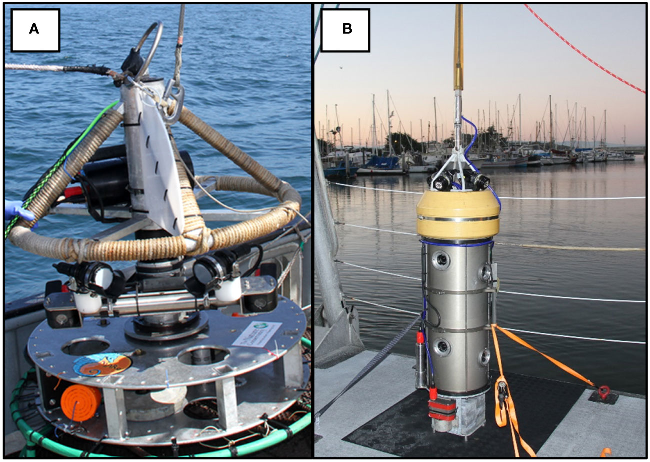
Figure 1 Schematic of video tools used to survey fishes on the continental shelf off California. (A) Rotating Lander and (B) Benthic Observation Survey System (BOSS).

In 2016, we started working with engineers and scientists from the Monterey Bay Aquarium Research Institute (MBARI) to develop a tool that addressed the issues with the first video lander. We conducted a design review with principal investigators from MBARI, MARE, and our project scientists that resulted in the development of the Benthic Observation Survey System (BOSS) tool (Figure 1B). The BOSS was built in a streamlined cylindrical shape to minimize resistance as it was lowered and raised in the water column, thus increasing speed of deployment and retrieval. The cylindrical design also limited the area of impact on the seafloor and made it easier to place the cameras close to rugose rocky habitats. Electronics and hardware are primarily internal to the cylinder, which minimizes damage due to contact with rock surfaces. The BOSS is equipped with four vertically-oriented camera pairs, mounted internally, and one down camera, mounted externally, that aids in lander placement on the seafloor (Figure 1B). All nine cameras are BlackMagic Design Micro Studio 4k cameras. There is a 24° gap in the field of view between each of the four camera pairs to prevent double-counting of fishes (Figure 2A). Each camera is toed in 7.5 degrees (vertically) to provide adequate camera overlap for stereo analysis (Figure 2B). Four lights (Deepsea Power & Light 160 W LED SeaLite, 3800 lumens) are mounted on top of the lander and a downward-facing light is mounted towards the bottom of the lander to help in placing the BOSS on the seafloor, up to its maximum operating depth of 400 m. The BOSS is controlled at the surface by a power distribution unit that generates the electrical power for the lander, decodes and distributes all video and data from the lander to computers on deck, and directly controls the cameras, lights, and other lander instrumentation via a touch screen.

Figure 2

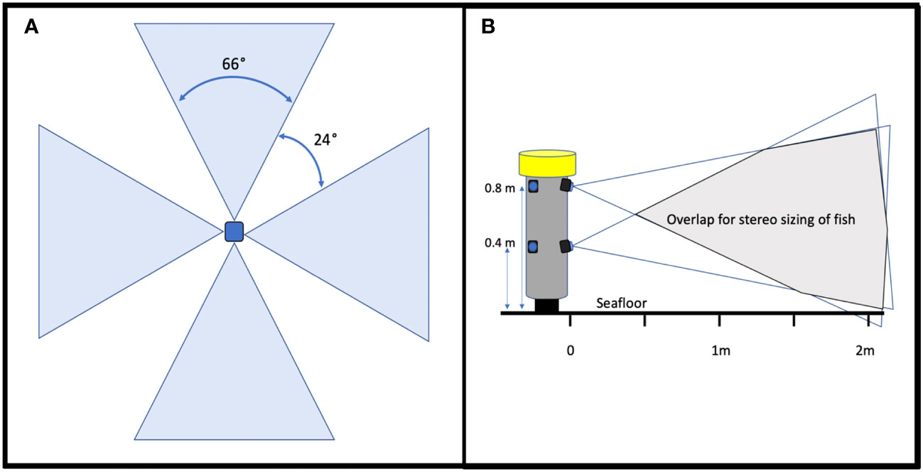
Figure 2 Schematic of (A) BOSS field of view and (B) stereo overlap. Cameras pointed down are considered to be the “top” cameras while cameras pointed up are considered the “bottom” cameras.

The BOSS is equipped with internal pressure and temperature sensors, as well as an externally mounted altimeter that reports the absolute depth of the lander as well its distance from the seafloor. A stabilizing fin is attached to one of the sides to minimize rotations when the BOSS is towed in the water column. We attach 68 kg of lead bricks to the base and 90 kg of flotation at the top of the lander prior to deployment so that the video lander remains vertical while on the seafloor. The BOSS is connected to a load-bearing fiber optic cable (operating strength 200 kg, breaking strength 1200 kg) that contains two optical fibers for video transmission and telemetry data as well as two large-gauge copper wires for electrical power. The cable is composed of an outer jacket made of 90C poly urethane, an inner Kevlar weave to provide strength, a thin polyester tape wrap, an elastomeric waterblock, two single-mode simplex fibers, and two 16AWG stranded tinned copper wires with 90C polypropylene insulation. The cable transfers video to the surface for real-time viewing and for recording on computer hard drives. The BOSS is deployed by an electric winch, designed by Okeanus Science and Technology LCC. The cable can be hauled in at 40 m per minute or payed out at a maximum speed of 59 m per minute. We have most often deployed the BOSS off an A-frame on the vessel’s stern, but occasionally have deployed the BOSS off a large davit on the side of a vessel. Although dynamic ship positioning systems make holding station above a video lander on the seafloor easier, the short time the BOSS is on the seafloor (<5 min) has enabled us to deploy the BOSS from ships with two propellers or one propeller and a bow thruster. See Supplementary Materials for more detail on the BOSS specifications.

2.2 Survey study area and deployment process

We conducted this study across the central and southern coast of California, USA, from Point Reyes to San Clemente Island (Figure 3). This area is characterized by cold water that flows from the sub-arctic to the equator via the California Current. The headland at Point Conception creates a biogeographic boundary between central California and the Southern California Bight, which is characterized by warmer waters to the east and colder waters to the west. The study area includes a variety of habitats, including flat, sandy seafloors, rocky outcrops and pinnacles, and mixed habitats with sand and cobble or boulders. We used the two types of video landers across the study area to survey primarily rocky habitats in depths from 40–345 m. These depths correspond to typical depths of recreationally and commercially harvested fishes on the continental shelf and slope in California.

Figure 3

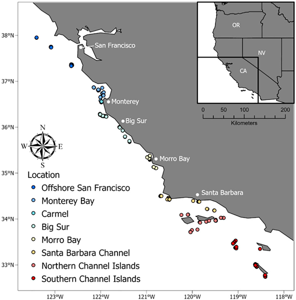
Figure 3 Location of BOSS and Rotating Lander video samples along the California coast that occurred on rocky habitats and in water depths less than 120 m.

Each time a video lander is put in the water is considered a “Deployment”. After Deployment, the video lander is lowered to 10 m above the seafloor. At that time, the downward light is turned on and the winch operator lowers the camera to the seafloor, pausing to ensure the camera system is placed within 1–2 m of rock outcrops. Once the video lander is stationary on the seafloor, we record the GPS location of the ship, wait for one minute to allow debris to settle, start the video recording, turn the video lights on, and label the spot as a “Drop” on our GIS software. Once the video sample is recorded (10–12 minutes for the rotating lander, 3–5 minutes for the BOSS), we turn the camera and lights off, bring the camera system 10–15 m off the bottom, and tow it to a new location, generally 75–500 m away from the previous Drop. Lights are turned off while towing the lander to a new location to avoid attracting fish. A Deployment will usually contain 5–15 Drops before the video lander is brought on board and the ship is moved to a new study location. Rotating Lander and BOSS video surveys occurred during the months of June, July, September, and October.

2.3 Video analysis and data extraction

We analyzed all videos using EventMeasure software (SeaGIS, Australia). For each Drop, we identified fish to the lowest taxonomic level and calculated MaxN for each species. In the case of the rotating lander, MaxN was defined as the maximum number of fish enumerated in one complete rotation. For the BOSS, a software program developed by SeaGIS, Inc., combined (stitched) video from the four bottom cameras into one “video frame” and the four top cameras into another video frame for analysis. These two video frames were synced together by time for analysis of MaxN. MaxN was defined as the maximum number of individuals of each species in a single corresponding video frame from all cameras during a recording (Figure 4). MaxN is a commonly used metric for stationary video cameras, as it eliminates the possibility of double-counting fish (Langlois et al., 2010). The total lengths of observed fishes were measured within the MaxN frame for as many species as possible. Fish that were too blurry, not within both stereo-camera frames, or at a large oblique angle to the camera were not measured.

Figure 4

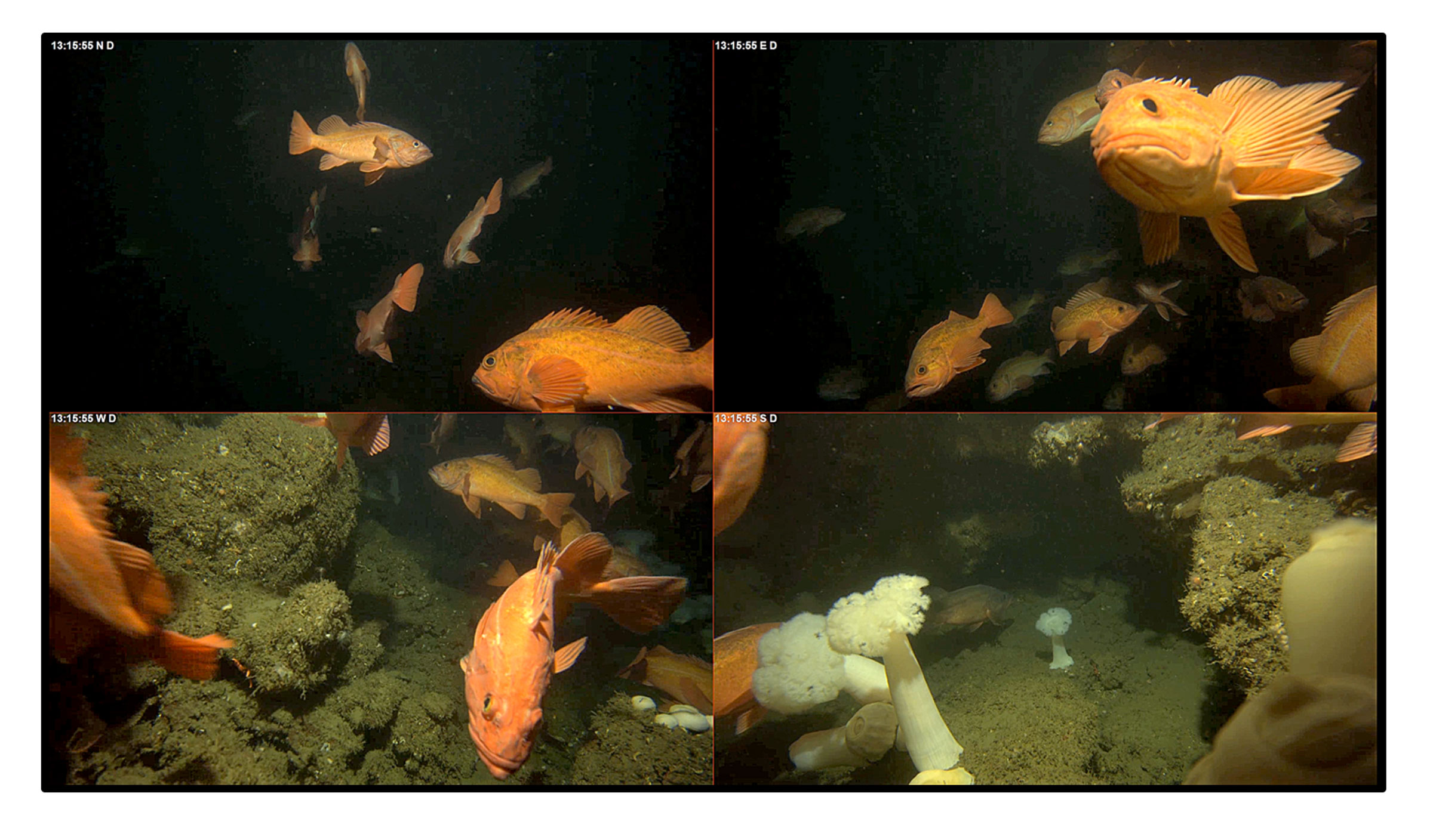
Figure 4 Example of corresponding video frames from the four bottom cameras on the BOSS that were stitched together in EventMeasure software for use in calculating MaxN and measuring fish lengths from stereo video pairs.

2.4 Data preparation

From 2013–2015, we deployed the Rotating Lander 459 times and collected data from 1,331 Drops. Most of those data were derived from baited drops, however, so here we only report Rotating Lander Drops that were not baited for comparison with BOSS Drops. BOSS surveys from 2018–2021 yielded a total of 1,113 Drops from 89 Deployments. We provide analyses of surveys occurring only in water depths from 40–120 m, in order to allow us to combine data from the two video landers, while avoiding variability caused by differences in community assemblages known to occur between the continental shelf and slope. In addition to depth restrictions, the Rotating Lander and BOSS data were filtered to contain only those drops that occurred in similar habitat, i.e., rock ridges or boulder habitats as opposed to sandy bottom habitats littered with cobble fields (see Tissot, 2008 for a description of habitats). Ultimately, we used 109 Rotating Lander Drops and 461 BOSS Drops for data analysis. We lumped Drops occurring geographically close to one another (within a radius of 50 km) that we believed would have similar habitat types, into a grouping we label “Location” (Figure 3).

Although the point-count method of estimating fish abundance provided similar metrics (i.e., MaxN and density) for data collected from each video lander, we used non-metric Multidimensional Scaling (nMDS) analysis to determine if there was a bias between the two tools. nMDS plots based on relative abundance among Locations and between tools indicated that there were greater differences among Locations than between tools (Figure 5). That, in combination with the similarities between tools and survey methods, led us to combine these datasets for use in our analyses.

Figure 5

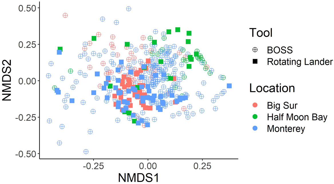
Figure 5 nMDS plot of Bray-Curtis dissimilarity matrix of square-root transformed, relative species abundance from BOSS and Rotating Lander tools. Locations used for the nMDS include Monterey, Big Sur, and Half Moon Bay sampling sites on rocky habitats and in water depths of less than 120 m. These locations were chosen because they contained numerous samples (Drops) from both survey tools.

2.5 Statistical analyses

All statistical analyses were performed in R v4.0 using the ‘vegan’ R package v2.6-4. To estimate the efficiency of our video landers compared to an ROV, we compared the average number of fish observed per minute for our video landers and an ROV at Monterey Bay and Carmel sampling locations. We chose these locations as there was spatial overlap among all the tools. The ROV was built by Deep Ocean Engineering and Research and operated by MARE. They conducted 500 m long transects with the ROV and counted all fishes observed in a 2 m field of view (Karpov et al., 2012). We divided the number of fish observed in the transect by the ROV’s average speed of 0.375 m/s to calculate the number of fish observed per minute on each transect. For the BOSS and Rotating Lander samples (Drops), we either used a 3 min total time or 8 min total time, respectively, and the MaxN for each Drop to calculate the number of fish observed per minute per sample. A Welch’s ANOVA test was used to compare differences in fish observed per minute between the tools.

Density was calculated as MaxN per drop, divided by the area surveyed. The area surveyed was determined by water visibility and the portion of a circle surveyed, as described in Starr et al. (2016). EventMeasure assigned every measurement a Z value, which is the Euclidean distance from the selected fish to the center of the plane containing each stereo camera pair. We calculated a 95% Z value, or the distance at which 95% of all individuals were observed based on a frequency distribution of individual fish distances. We chose this value to be the conservative maximum distance that we could accurately identify an individual fish across a variety of seafloor conditions (water visibility, terrain ruggedness, etc.). Fish observations that fell outside of the 95% Z distance were omitted from analyses. For all species observed less than 10 times, 95% Z was calculated based on the distance of all species combined. For species with greater than 10 measurements, area was calculated based on the species-specific 95% Z (Starr et al., 2016).

We calculated the coefficient of variation (standard error/mean) in species density in each Location (cluster of drops) and plotted the bootstrapped data across sampling effort to determine the minimum number of surveys that resulted in an 80% reduction in variability of the estimate (Figure 6). The minimum number of drops differed among Locations; however, we chose 25 drops as a conservative minimum sample size needed in each Location. Species abundance data were bootstrapped to account for uneven sample sizes. All Drops from one Location were aggregated together to create sample replicates. Twenty-five Drops were randomly selected from the sample replicates to create a sample unit in which species metrics were calculated. This was repeated 100 times, with resampling. Species richness (S), relative abundance (density), Shannon’s diversity index (H’) (Shannon and Wiener, 1963), and Pielou’s evenness (E’) (Pielou, 1975) were calculated for each sample unit. To test statistical differences in species richness, diversity, and evenness, we either performed a Kruskal-Wallis test to account for non-normality, or a Welch’s analysis of variance (ANOVA) to account for unequal variances. Differences between Locations were assessed with a Games-Howell test, a post hoc test used when there is a violation of the assumptions of normality and homogeneity of variance. We were specifically interested in developing an approach to detect differences in diversity and evenness indices to help identify rapidly changing biotic communities. This approach was highlighted by Trindade-Santos et al. (2020), who described a change in functional diversity of fished species and identified the importance of incorporating functional diversity in ecosystem management.

Figure 6

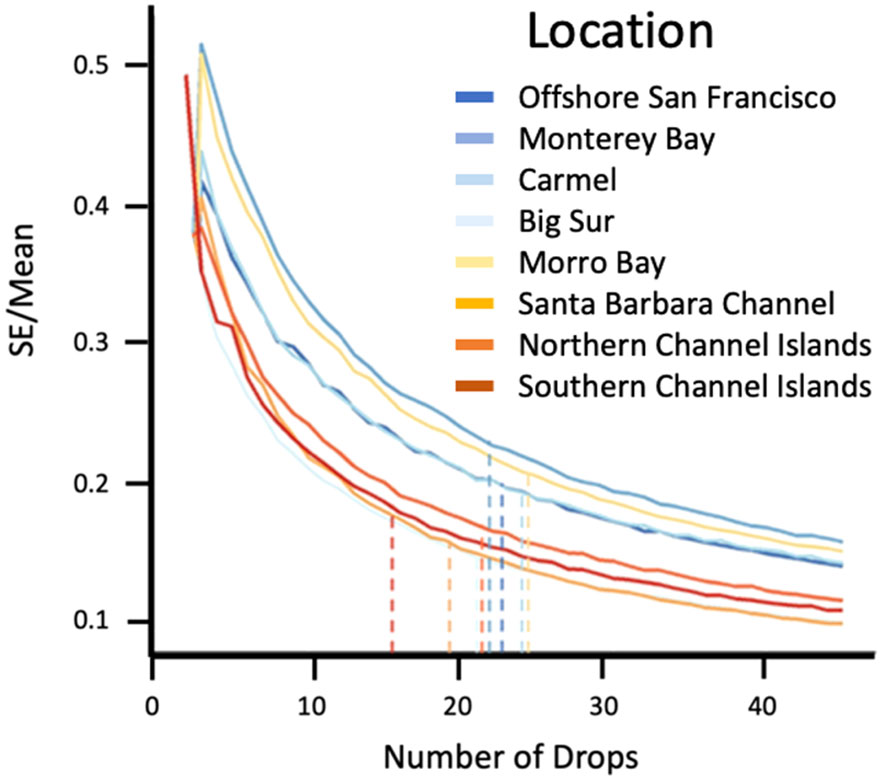
Figure 6 Coefficient of variation (SE/mean) of species density among Locations. Dotted lines indicate the number of Drops needed to reduce the variability by 80% at each sampling Location.

We generated a Bray-Curtis dissimilarity matrix and used nMDS plots to compare fish community composition among Locations. Relative abundance data were square-root transformed prior to use in the matrix. We used an unordered Analysis of Similarity (ANOSIM) with Location as a factor to investigate differences in community compositions among Locations. We also used a similarity of percentage (SIMPER) model to determine which species were driving the differences among Locations. Mean relative abundance (%) of the most abundant species was also calculated to ascertain species-specific differences in composition among Locations. To determine if there were fine-scale differences in species assemblages at a given Location, we investigated how community assemblages differed within a Location. We separated both the Monterey Bay and the northern Channel Islands locations into smaller clusters of Drops and created a nMDS plot from the Bray-Curtis dissimilarity matrix and assessed differences in community assemblages with an ANOSIM.

Fish length data were treated differently than community composition information. We did not bootstrap fish length data, rather we grouped fish length data from spatially different Locations to maximize sample sizes. We grouped Monterey Bay and Carmel to form a Monterey Bay “Region”. Similarly, fish lengths obtained from the Morro Bay were grouped with Big Sur to form a Big Sur Region. Fish lengths from the Santa Barbara Channel, northern Channel Islands, and the southern Channel Islands Locations were grouped together to form the Channel Islands Region. These combined sampling locations yielded four Regions that we used to investigate differences in fish lengths among the spatial areas of Offshore San Francisco, Monterey Bay, Big Sur, and the Channel Islands. Within these four Regions, differences in fish lengths were assessed for the five most frequently measured species. We used a nested permutational multivariate analyses of variance (PERMANOVA) using the Euclidean Distance dissimilarity measure on raw length data to compare differences in fish lengths among Regions. Drop was used as the nested random factor and Region as the fixed factor. The nested Drop factor was included as the number of fish measured varied between deployments (Bornt et al., 2015). We used the ‘pairwiseAdonis’ package V0.4.1 to identify pairwise comparisons among Regions.

3 Results

3.1 Video surveys

A total of 12,849 individual fish belonging to 18 families, 26 genera, and 65 species were identified to the species taxonomic level (Supplementary Table 1) from all locations, ranging from Offshore San Francisco in the northern part of the study area to the southern Channel Islands (Table 1). The most diverse family was Scorpaenidae (40 species), followed by Embiotocidae (4 species), and Hexagrammidae (3 species). All other families were represented by two or fewer species. The most abundant species were Squarespot Rockfish (Sebastes hopkinsi, n = 2,713), Yellowtail Rockfish (Sebastes flavidus, n = 1,580), Vermilion Rockfish (Sebastes miniatus, n = 1,230), Pygmy Rockfish (Sebastes wilsoni, n = 1,191), and Bocaccio (Sebastes paucispinis, n = 816). The species that occurred the most frequently were Vermilion Rockfish (present in 41% of drops), Squarespot Rockfish (40%), Bocaccio (37%), Lingcod (Ophiodon elongatus, 35%), Rosy Rockfish (Sebastes rosaceus, 33%), and Yellowtail Rockfish (33%).

Table 1

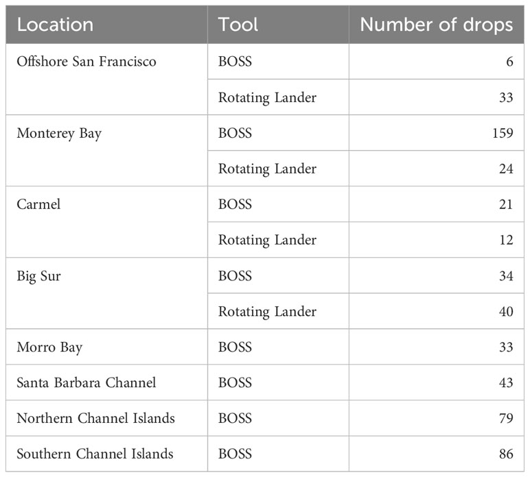
Table 1 Number of drops completed per tool in each location that were used in analyses.

We compared the number of Bocaccio, Canary Rockfish, Lingcod, and Vermilion Rockfish observed per minute between our video landers and the ROV. We chose these species due to their abundances in both datasets at each location. At the Carmel sampling location, we found that the BOSS and Rotating Lander observed more fish per minute on average than the ROV for Bocaccio (Welch’s ANOVA F_1,29 = 4.87, P = 0.04), Canary Rockfish (Welch’s ANOVA F_1,29 = 7.79, P = 0.01), Lingcod (Welch’s ANOVA F_1,50 = 6.53, P = 0.01), and Vermilion Rockfish (Welch’s ANOVA F_1,30 = 5.88, P = 0.02) (Supplementary Table 2). At the Monterey Bay sampling location, we found that the BOSS and Rotating Lander recorded more fish per minute on average than the ROV for Bocaccio (Welch’s ANOVA F_1,97 = 23.08, P < 0.001) and Vermilion Rockfish (Welch’s ANOVA F_1,54 = 6.12, P = 0.02) while the ROV observed more fish per minute on average than the BOSS and Rotating Lander for Lingcod (Welch’s ANOVA F_1,12 = 9.98, P = 0.01). Lastly, there was no difference between methods for Canary Rockfish (Welch’s ANOVA F_1,32 = 0.96, P = 0.33) (Supplementary Table 3).

3.2 Species richness, diversity, and evenness

Species richness varied across the coast and ranged from 15.54 ± 0.78 species per 25 drops in the Carmel Location to 33.39 ± 2.08 species per 25 drops in the southern Channel Islands (Table 2). In general, southern Locations exhibited a greater average richness than northern Locations, except for the case of Morro Bay (Figure 7A). These trends were verified using a Welch’s ANOVA (F_7,336 = 2456.8, P < 0.001). The southern Channel Islands exhibited the greatest species richness of all sites, while Carmel exhibited the least species richness (Supplementary Table 4).

Table 2

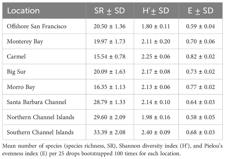
Table 2 Average diversity indices in each location.

Figure 7

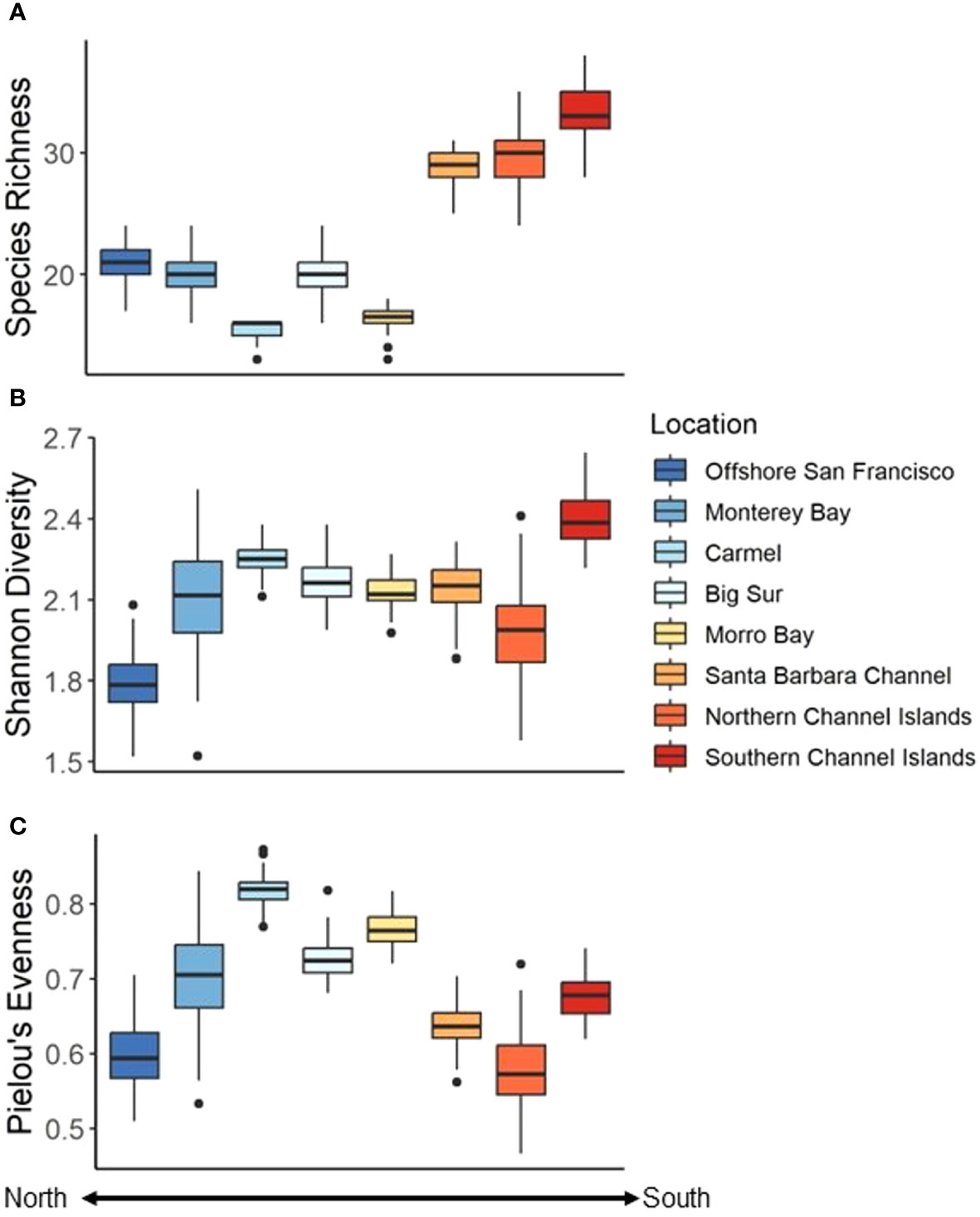
Figure 7 Diversity (per 25 Drops bootstrapped 100 times) indices among Locations. (A) Species richness, (B) Shannon diversity Index, and (C) Pielou’s evenness. Colder colors represent more northern Locations while warmer colors represent more southern Locations.

The Shannon Diversity Index also varied among Locations, and ranged from 1.79 ± 0.11 in Offshore San Francisco, to 2.40 ± 0.09 in the southern Channel Islands (Table 2, Figure 7B). There was a difference in diversity among Locations (Welch’s ANOVA, F_7,323 = 323.03, P < 0.001), though it was less pronounced than differences in species richness (Supplementary Table 3). The evenness of the communities was lowest in the northern Channel Islands (0.58 ± 0.05) and highest in the Carmel Location (0.82 ± 0.02) (Table 2, Figure 7C). Differences were found among Locations (Welch’s ANOVA, F_7,342 = 1165.6, P < 0.001), with Offshore San Francisco and the northern Channel Islands exhibiting the lowest species evenness and Carmel exhibiting the greatest species evenness (Supplementary Table 5).

3.3 Community assemblages

For both species abundance and density, nMDS analysis showed some similarity among Locations (Figure 8). Specifically, species in northern study Locations, such as offshore San Francisco and Half Moon Bay aggregated together while southern Locations, such as the Channel Islands, aggregated together. Species in Monterey Bay, Carmel, Big Sur, Morro Bay, and the Santa Barbara Channel study sites aggregated in the middle, which is logical because they are geographically located between the northern and southern Locations mentioned above.

Figure 8

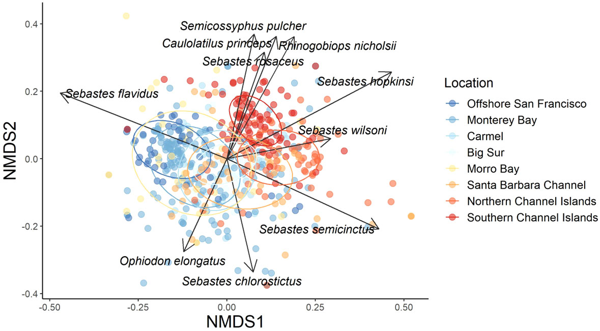
Figure 8 nMDS with species vectors of Bray-Curtis dissimilarity matrix of relative species abundance for sampling Locations across the California coast. The data were square root transformed and colder colors represent more northern Locations while warmer colors represent more southern Locations. Ellipses represent 95% confidence intervals. Stress = 0.19.

The ANOSIM of the species compositions showed a significant difference among Locations (R = 0.28, P = 0.001; Table 3). All Locations were significantly different (P < 0.05) from one another except for Monterey Bay and Offshore San Francisco (R = 0.02, P = 0.72), Monterey Bay and Big Sur (R = 0.013, P = 0.28), and Monterey Bay and Carmel (R = 0.03, P = 0.23). The Locations that exhibited the greatest difference in community assemblages were Offshore San Francisco and the southern Channel Islands (R = 0.74, P <.001), Morro Bay and the southern Channel Islands (R = 0.67, P <.001), and Offshore San Francisco and the northern Channel Islands (R = 0.67, P <.001).

Table 3

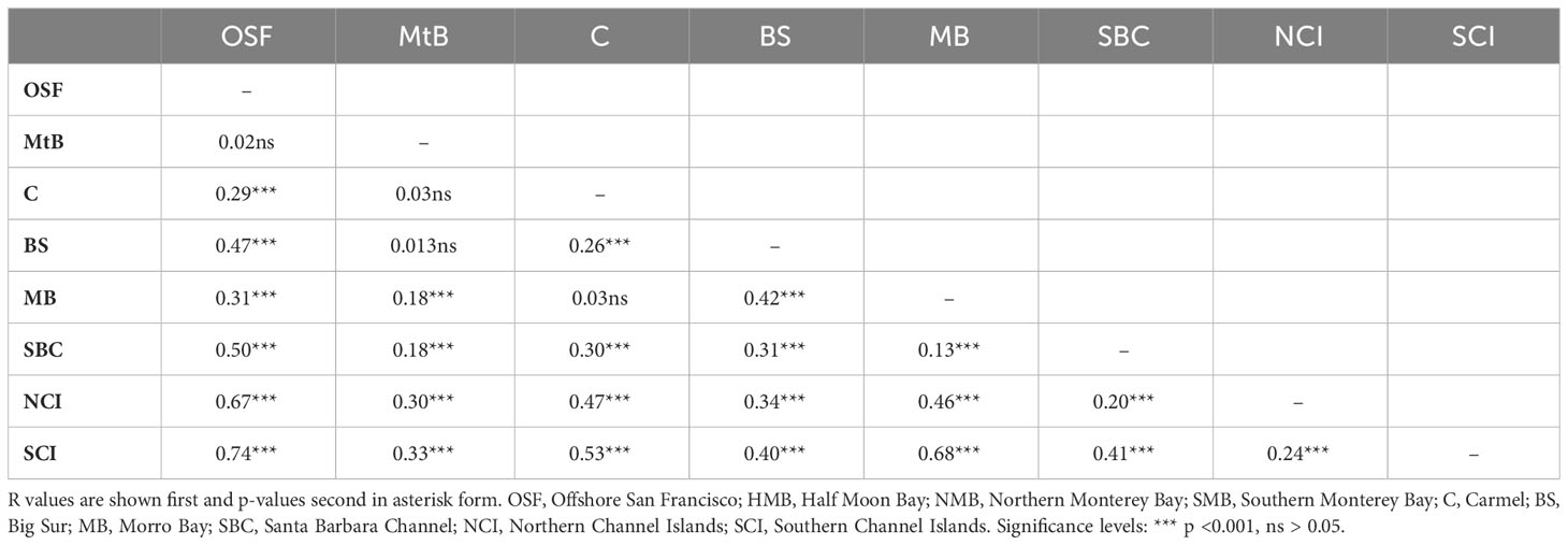
Table 3 One-way ANOSIM test for variation in community assemblages among locations.

The greatest differences between Locations from the SIMPER analysis were between the Northern Channel Islands and Offshore San Francisco (Supplementary Table 6). The differences were driven by Squarespot Rockfish, Yellowtail Rockfish, Halfbanded Rockfish, Canary Rockfish, and Pygmy Rockfish. The Locations that were the most similar were Big Sur and Carmel, with differences being driven by Vermilion Rockfish, Pygmy Rockfish, Squarespot Rockfish, Canary Rockfish, and Yellowtail Rockfish (Supplementary Table 6).

Yellowtail Rockfish was the most abundant fish species observed in the northern Locations of Offshore San Francisco and Monterey Bay (Figure 9). Canary Rockfish (Sebastes pinniger) were also prevalent in the northern Locations, but were rarely seen south of Big Sur. At Big Sur, Vermilion Rockfish, Squarespot Rockfish, and Pygmy Rockfish comprised the majority of the fish community. Further south, Vermilion Rockfish mean relative abundance decreased while Squarespot Rockfish mean relative abundance increased. Halfbanded Rockfish (Sebastes semicinctus) comprised a large percentage of mean relative abundance from Morro Bay to the northern Channel Islands. Different species appeared in the Southern locations, such as Ocean Whitefish (Caulolatilus princeps) and Blacksmith (Chromis punctipinnis). Some of these patterns are mirrored in the species vectors of the nMDS, with Canary Rockfish, Greenspotted Rockfish (Sebastes chlorostictus), and Yellowtail Rockfish as the most influential species in the more northern locations, but with Squarespot Rockfish, Ocean Whitefish, California Sheephead (Semicossyphus pulcher), and Blackeye Goby (Rhinogobiops nicholsii) as the most influential species in the southern locations. The ubiquitous Halfbanded Rockfish was also commonly observed from Morro Bay to the northern Channel Islands.

Figure 9

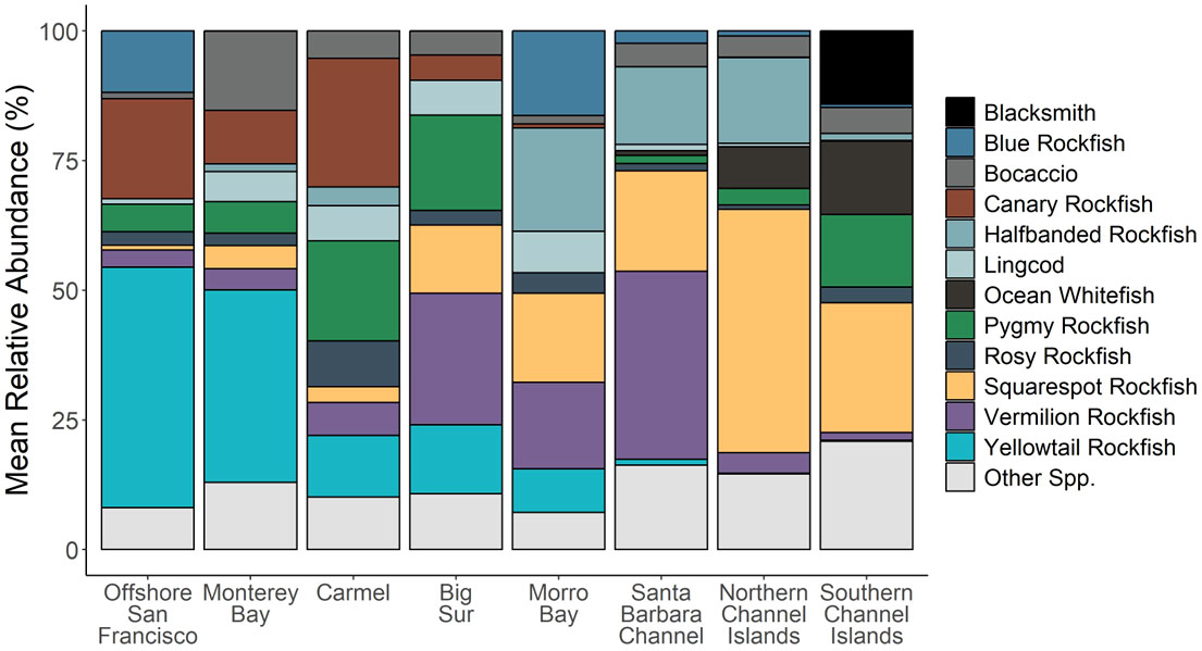
Figure 9 Mean relative abundance (percentage of the total number of species observed) of the 12 most commonly observed species across all surveys in each Location. All other species were grouped together to form the “Other” category.

3.4 Fish lengths and densities

A total of 3,773 lengths from individual fish identified to species were obtained from video measurements. The species measured most frequently were Yellowtail Rockfish (n = 789 individuals), Vermilion Rockfish (n = 544), Canary Rockfish (n = 408), Bocaccio (n = 254), and Lingcod (n = 168) (Supplementary Table 6). These species exhibited differences in length among Regions (Figure 10). Using a PERMANOVA, we identified significant differences in lengths among Regions for Bocaccio (F₃ = 34.65, P = 0.001), Canary Rockfish (F₂ = 191.49, P = 0.001), Vermilion Rockfish (F₃ = 40.13, P = 0.001), Yellowtail Rockfish (F₃ = 60.11, P = 0.001), and Lingcod (F₃ = 5.66, P = 0.004). Specifically, Bocaccio were larger in Monterey Bay and Big Sur than any other Region (P < 0.05). Canary Rockfish were the smallest in Offshore San Francisco (P < 0.05), and the largest in the Channel Islands Region (P < 0.05). Vermilion Rockfish were smaller in the Channel Islands than any other Region (P < 0.05). Yellowtail Rockfish were larger in Big Sur than either Offshore San Francisco Bay or Monterey Bay. Lastly, Lingcod in Big Sur were larger than Lingcod in the Monterey Bay Region (P < 0.05).

Figure 10

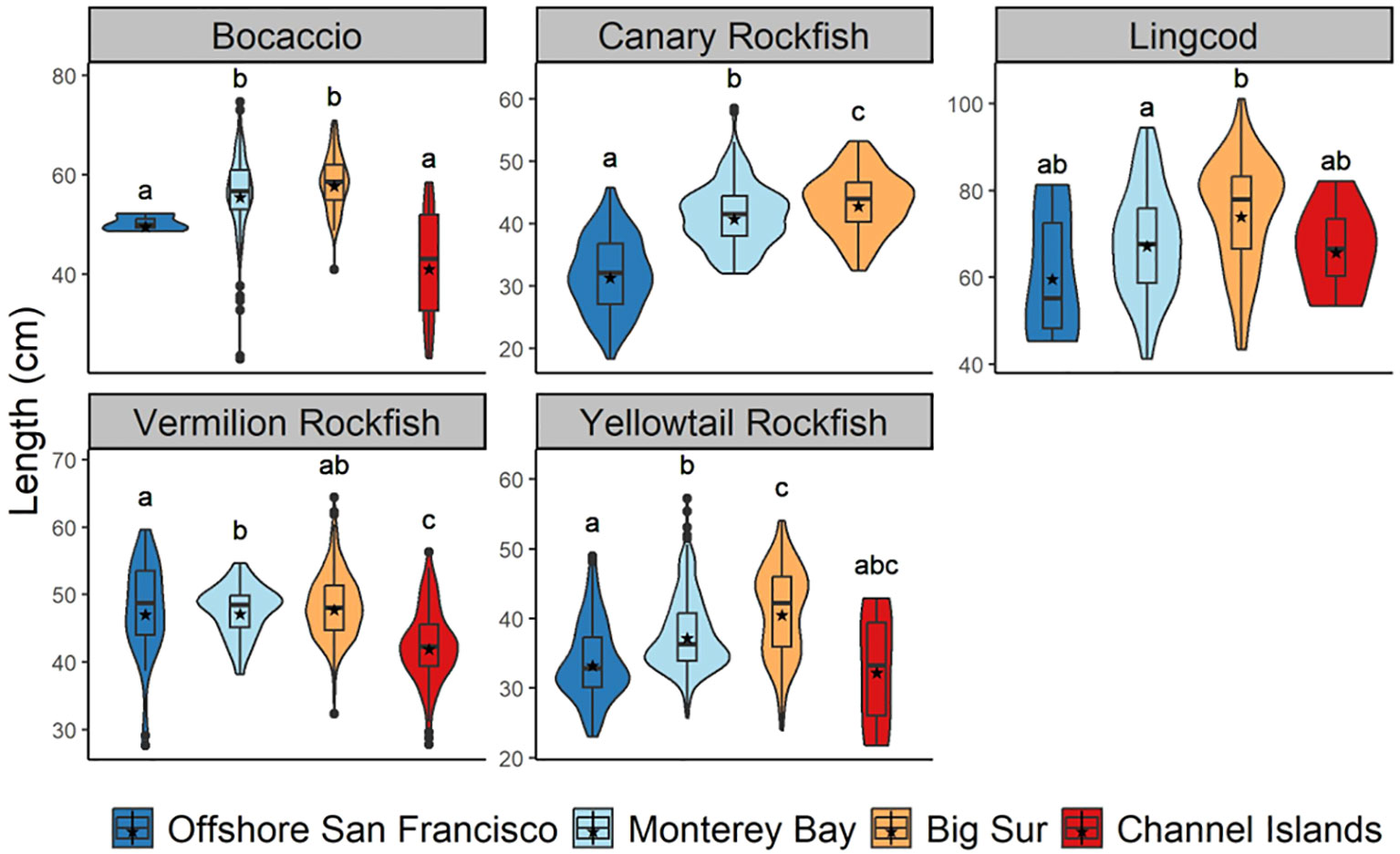
Figure 10 Lengths (cm) of Bocaccio, Canary Rockfish, Lingcod, Vermilion Rockfish, and Yellowtail Rockfish. Regions include Offshore San Francisco, Monterey Bay, Big Sur, and the Channel Islands. Stars represent mean lengths and different letters indicate statistically significant differences (p<0.05).

Bocaccio, Canary Rockfish, Lingcod, Vermilion Rockfish, and Yellowtail Rockfish all exhibited different trends in density along the coast (Figure 11). Densities of Canary Rockfish and Yellowtail Rockfish were higher in the northern areas compared to the southern areas while Lingcod and Vermilion Rockfish exhibited higher densities in the middle locations. Finally, Bocaccio exhibited higher densities at both northern and southern sampling sites. A Welch’s ANOVA determined significant differences in density among locations for Bocaccio (F_7,15 = 3.04, P = 0.03), Lingcod (F_7,40 = 27, P < 0.001), Vermilion Rockfish (F_7,71 = 8.03, P <0.001), and Yellowtail Rockfish (F_7,16 = 7.10, P < 0.001). Bocaccio densities at the Monterey Location were higher than at Offshore San Francisco or Big Sur Locations (Games – Howell P < 0.05). Lingcod exhibited the highest densities at Monterey, Carmel, Big Sur, and Morro Bay Locations, and the lowest densities at Offshore San Francisco, the northern Channel Islands, and the southern Channel Islands Locations (Games – Howell P < 0.05). Vermilion Rockfish exhibited the highest densities at the Santa Barbara Channel location followed by the Big Sur Location (Games – Howell P < 0.05). Lastly, Yellowtail Rockfish exhibited the highest densities at the Monterey Bay Location (Games – Howell P < 0.05).

Figure 11

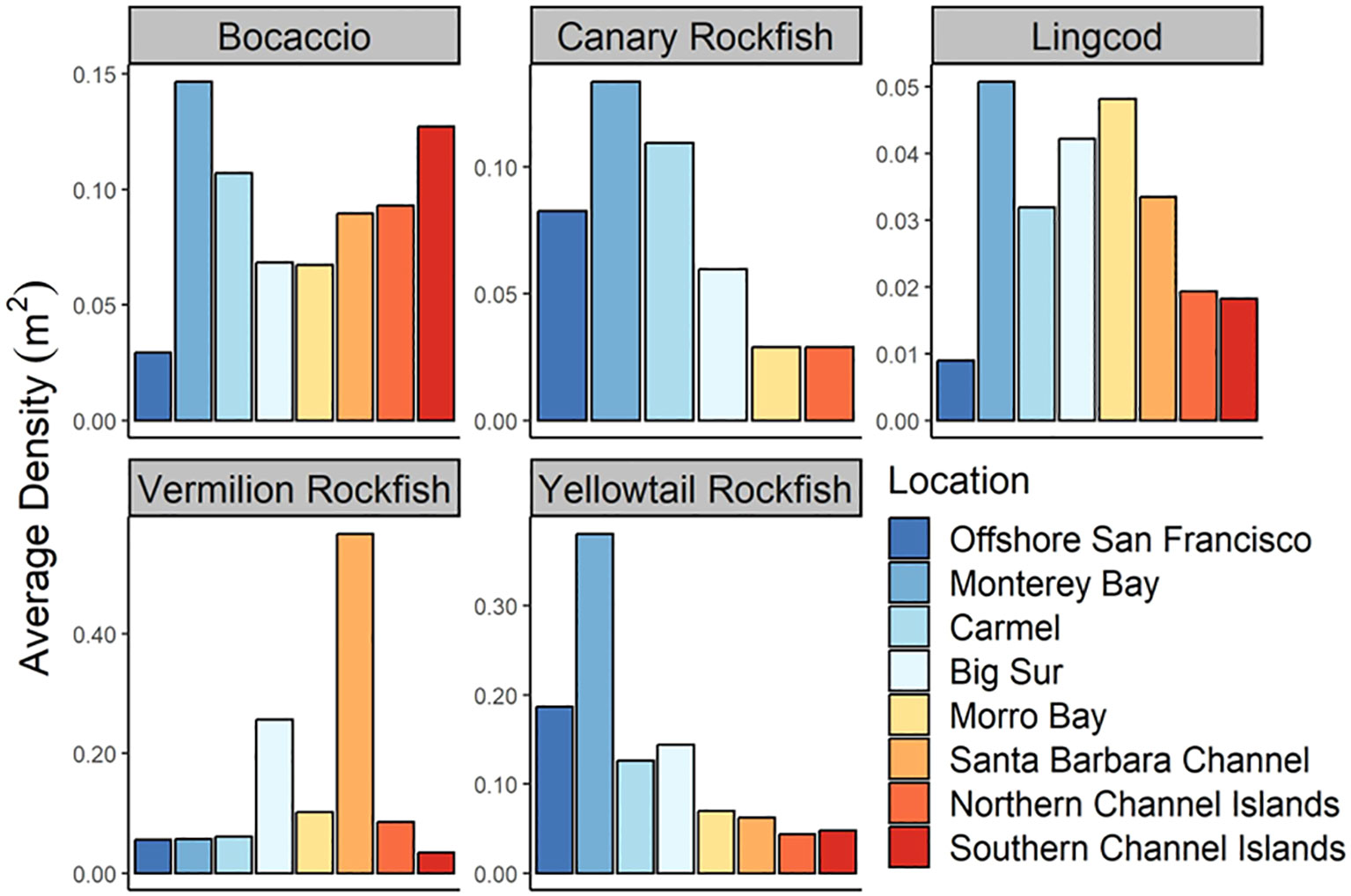
Figure 11 Density (fish/m²) of Bocaccio, Canary Rockfish, Lingcod, Vermilion Rockfish, and Yellowtail Rockfish among Locations.

3.5 Fine-scale spatial differences in species composition

Five specific clusters of Drops, hereby called “Groups” occurred within the Monterey Bay and Carmel locations (labeled A-E, Figure 12). These Groups were examined further to determine if there were fine-scale differences in species composition within Monterey Bay. The ANOSIM of the species compositions resulted in significant differences among the Groups in Monterey Bay (R = 0.314, P = 0.001; Supplementary Table 7). All Groups were significantly different from one another, besides Groups A and B (R = 0.12, P = 0.14), and Groups B and C (R = 0.08, P = 0.22). The Groups that exhibited the largest difference in community composition were A and D (R = 0.41, P = 0.001), and C and D (R = 0.39, P = 0.001). Within the northern Channel Islands, there were also five Groups that were analyzed further to determine ecological differences in community structure (Figure 12). An ANOSIM revealed that there were significant differences among the Groups (R = 0.19, P = 0.001; Supplementary Table 8). The pairwise comparisons that exhibited the largest differences in community assemblages were Groups B and C (R = 0.30, P < 0.01), and Groups D and E (R = 0.31, P < 0.05).

Figure 12

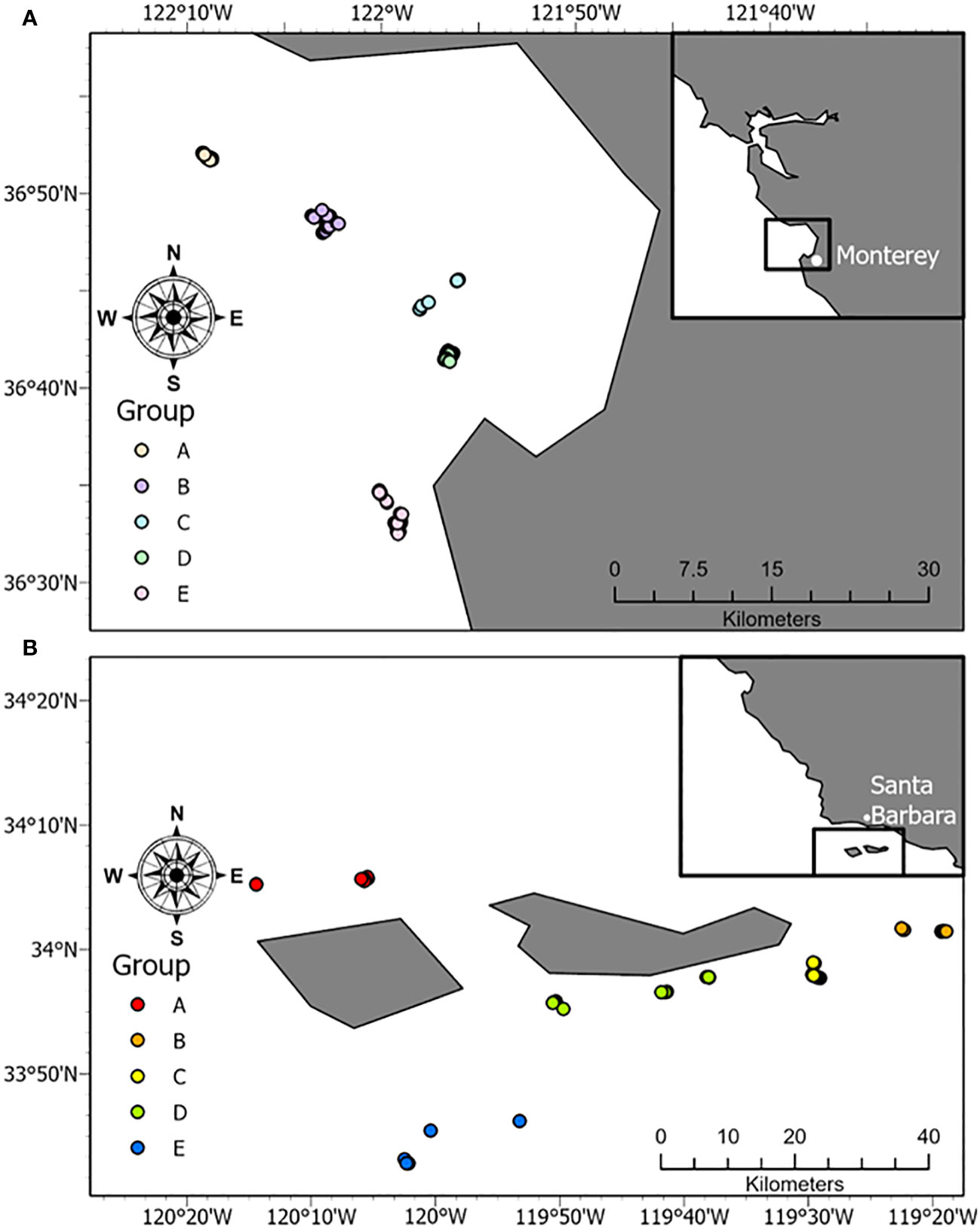
Figure 12 Unique Groups of 25 or more Drops located in (A) Monterey Bay and (B) the northern Channel Islands.

4 Discussion

As evidence mounts that the rate of climate change is accelerating (Masson-Delmotte et al., 2021), we suggest that new tools are needed to quickly identify and evaluate the associated changes in biodiversity. We developed stereo-video camera systems that could be used to quickly evaluate spatial differences among fish community assemblages within a similar depth range and habitat throughout central and southern California. Our surveys provided similar information about species distributions and habitat associations to those derived from submersible surveys in California (Yoklavich et al., 2002; Starr and Yoklavich, 2008; Love et al., 2009; Wedding and Yoklavich, 2015). Rockfishes dominated both the high- and low-relief rock habitats we surveyed, however other species such as Ocean Whitefish, Blacksmith, and California Sheephead were also important components of the fish communities in southern California. Love et al. (2009) reported that species richness peaked at depths of 50–125 m, with the number of species declining linearly out to the maximum depths of their study (365 m). Similar to species richness, fish density in our study was highest in the 50–125 m depth zone and decreased with increasing depth. In addition, fishes were larger in the deeper parts of the survey locations. Wedding and Yoklavich (2015) reported similar trends of decreasing densities with depth on the continental slope for rockfishes in central California.

Overall, we detected differences in diversity metrics among several biogeographic regions and Locations along the California coastline along with species-level differences in lengths and densities. We determined that there were differences among diversity metrics throughout central and southern California. In general, southern Locations exhibited a higher species richness than all other locations; however, southern Locations did not consistently exhibit the highest species diversity. Other studies have shown that depth and substrate (habitat) are often found to be more important than latitude when explaining patterns in diversity (Levin et al., 2001; Tolimieri and Levin, 2006; Piacenza et al., 2015; Rex et al., 2000). However, even within the same depth zone and habitat, we found that species diversity changed on a relatively small spatial scale. This may be because temperature and currents, which are important drivers of diversity, exhibit fine-scale variation, both spatially and temporally. For example, Amaya et al. (2023) reported that marine heatwaves did not follow a linear relationship with depth along the California Current, but peaked around 100 m depth. Bottom water temperatures can be influenced by internal oceanographic currents, marine heatwaves, and upwelling (Wang et al., 2021). Furthermore, there is a large temperature gradient surrounding the Channel Islands, with eastern islands experiencing warmer water temperatures than western islands (Hickey, 1992). In addition, fishes could be associated with finer-scale habitat differences not accounted for in our study. Consequently, it is logical that species diversity in mid-depth regions off the coast of California is more nuanced and dependent upon multiple factors.

We also found that length distributions of fishes differed across the coast, which could indicate spatial differences in recruitment, and/or differences in rates of growth or mortality. Spatial differences in recruitment could be caused by bottom-up processes such as juvenile survival triggered by spatial differences in ocean productivity. Alternatively, differences in length frequencies could be caused by differential adult mortalities due to predation, disease, or movements of adults. Long-term plankton surveys have shown major shifts in the settlement patterns of juvenile rockfishes, and that the abundance of winter-spawning rockfishes is highly variable over space and time (Field et al., 2021). This is not surprising in the dynamic CCE, and reiterates the need for tools that can be used to quickly identify temporal and spatial changes in community assemblages across various spatial scales. In addition to changes in recruitment, a shift in the distribution of lengths can be an indicator of a changing environment. As climate change causes water temperatures to increase, fish body size can shift to either larger sized individuals or smaller sized individuals (Audzijonyte et al., 2020). These variable changes in the length distributions of fishes, if occurring in the CCE, need to be studied to ascertain how the community size composition is changing in the face of climate change. Understanding how the size distributions of fishes change with temperature could have implications for interpreting stock assessments that use the size distribution of fishes to estimate a given population size.

Our results showed that fish community assemblages varied spatially along the California coastline. Love et al. (2002) described a gradient in rockfish species richness from north to south. Our data did not show linear trends in differences along bioregions, but rather variations within a bioregion that we believe are due to differences in habitat, small-scale oceanographic processes, and stochastic settlements of juvenile fish. Northern areas were mostly dominated by Canary Rockfish and Yellowtail Rockfish while southern areas were dominated by Squarespot Rockfish and Vermilion Rockfish. This is consistent with Marks et al. (2015) who used hook and line sampling to determine that species composition at both the Farallon Islands and Half Moon Bay was dominated by Yellowtail Rockfish, Blue Rockfish (Sebastes mystinus), and Canary Rockfish. Submersible studies conducted north of Monterey also reported high abundances of Yellowtail Rockfish (Laidig et al., 2009).

Our results not only demonstrate differences in community assemblages among California bioregions, but also variations within Locations. For example, we found differences in community assemblages within Monterey Bay and the northern Channel Islands that could, in part, be explained by small-scale variations in the topography or complexity of rocky habitat. Topographic metrics derived from remote sensing tools, such as slope and rugosity, describe the complexity or topography of the seafloor (Kuffner et al., 2007; Walker et al., 2009; Brown et al., 2019). Researchers have found that specific fish species off California associate with certain values of topographic metrics (Young et al., 2010; Young and Carr, 2015; Matthews, 2023). These associations with specific traits of rocky reef features could help to explain why we detected differences in community assemblages within rocky habitats of a Location.

The ability to rapidly survey large areas for changes in community assemblages will become increasingly more important in California, and globally, as natural and anthropogenic factors threaten the stability of these communities. For example, perturbations in ocean currents and productivity are expected to increase in frequency and magnitude as the earth experiences global climate change (Grimm et al., 2013), which could alter fish community assemblages. In addition, community assemblages off California could change soon due to decommissioning of oil platforms, offshore wind development, changes in commercial and recreational fishing, and increased protected areas. We suggest that relatively inexpensive and easy to operate stereo-video tools, used in conjunction with a point-sampling survey design, can effectively detect differences in fish community assemblages and biodiversity patterns across multiple scales in rocky, high-relief habitats. Some of the specific benefits of the BOSS system include quick deployment, a relatively high sampling rate, a live video feed to the surface, relatively lower costs, stereo-video capability, and the ability to target certain habitats over large areas.

Data availability statement

The raw data supporting the conclusions of this article will be made available by the authors, without undue reservation.

Ethics statement

The manuscript presents research on animals that do not require ethical approval for their study.

Author contributions

KM: Data curation, Formal Analysis, Visualization, Writing – original draft, Writing – review & editing, Investigation, Validation. RF: Data curation, Writing – review & editing, Investigation, Methodology, Project administration, Validation. KC: Data curation, Writing – review & editing, Investigation, Project administration, Validation. JM: Writing – review & editing, Data curation, Investigation, Project administration, Validation. MG: Conceptualization, Funding acquisition, Investigation, Methodology, Writing – review & editing. RS: Writing – original draft, Writing – review & editing, Conceptualization, Funding acquisition, Investigation, Methodology, Project administration, Supervision.

Funding

The author(s) declare financial support was received for the research, authorship, and/or publication of this article. Funding for the video lander projects came from a variety of sources. The Nature Conservancy (SJSU Tower Foundation Grant Account 23-1509-2603 and 23-1509-2649) and private funders, including the David and Lucile Packard Foundation, provided support throughout the development and use of the video lander tools. The Monterey Bay Aquarium Research Institute provided support for the engineers and technicians who worked on the BOSS project. We also received funds from the NOAA SK funding program (NOAA Award NA17NMF4270215 and NA20NMF4270166), and the California Sea Grant Program and the California Ocean Protection Council (R/MPA-48).

Acknowledgments

We would like to thank researchers for their work at sea conducting video surveys and for analyzing video data (Corina Marks, Donna Kline, Christian Denney, Anne Tagini, Jake Todd, and Molly Alvino). Marine Applied Research and Exploration (Dirk Rosen, Rick Botman, Andy Lauermann, and David Jeffries) designed, built and maintained the rotating lander system while Chad Kecy, Francois Cazenave, Eric Martin, Craig Okuda and Kent Headly of the Monterey Bay Aquarium Research Institute designed, built and maintained the Benthic Observation Survey System. We would also like to thank Jim Seager of SeaGIS for his help and support of our Cal and EventMeasure software. Additionally, we received help from the skippers and crew of the FV Donna Kathleen, the RV Fulmar, the RV Shearwater, the RV John Martin, and the CPFV Outer Limits. We thank the external reviewers for providing suggestions that improved the manuscript.

Conflict of interest

The authors declare that the research was conducted in the absence of any commercial or financial relationships that could be construed as a potential conflict of interest.

Publisher’s note

All claims expressed in this article are solely those of the authors and do not necessarily represent those of their affiliated organizations, or those of the publisher, the editors and the reviewers. Any product that may be evaluated in this article, or claim that may be made by its manufacturer, is not guaranteed or endorsed by the publisher.

Supplementary material

The Supplementary Material for this article can be found online at: https://www.frontiersin.org/articles/10.3389/fmars.2024.1368083/full#supplementary-material

References

Amaya D. J., Jacox M. G., Alexander M. A., Scott J. D., Deser C., Capotondi A., et al. (2023). Bottom marine heatwaves along the continental shelves of North America. Nat. Commun. 14, 1038. doi: 10.1038/s41467-023-36567-0

PubMed Abstract | CrossRef Full Text | Google Scholar

Anderson T. J., Syms C., Roberts D. A., Howard D. F. (2009). Multi-scale fish-habitat associations and the use of habitat surrogates to predict the organization and abundance of deep-water fish assemblages. J. Exp. Mar. Bio. Ecol. 379, 34–42. doi: 10.1016/j.jembe.2009.07.033

CrossRef Full Text | Google Scholar

Audzijonyte A., Richards S. A., Stuart-Smith R. D., Pecl G., Edgar G. J., Barrett N. S., et al. (2020). Fish body sizes change with temperature but not all species shrink with warming. Nat. Ecol. Evol. 4, 809–814. doi: 10.1038/s41559-020-1171-0

PubMed Abstract | CrossRef Full Text | Google Scholar

Auster P. J., Giacalone L. (2021). Virtual reality camera technology facilitates sampling of interactions between reef piscivores and prey. Mar. Technol. Soc 55, 54–63. doi: 10.4031/MTSJ.55.2.1

CrossRef Full Text | Google Scholar

Bornt K. R., McLean D. L., Langlois T. J., Harvey E. S., Bellchambers L. M., Evans S. N., et al. (2015). Targeted demersal fish species exhibit variable responses to long-term protection from fishing at the Houtman Abrolhos Islands. Coral Reefs 34, 1297–1312. doi: 10.1007/s00338-015-1336-5

CrossRef Full Text | Google Scholar

Brooks E. J., Sloman K. A., Sims D. W., Danylchuk A. J. (2011). Validating the use of baited remote underwater video surveys for assessing the diversity, distribution and abundance of sharks in the Bahamas. Endanger. Species Res. 13, 231–243. doi: 10.3354/esr00331

CrossRef Full Text | Google Scholar

Brown C. J., Beaudoin J., Brissette M., Gazzola V. (2019). Multispectral multibeam echo sounder backscatter as a tool for improved seafloor characterization. Geosciences 9, 126. doi: 10.3390/geosciences9030126

CrossRef Full Text | Google Scholar

Cappo M., Harvey E., Shortis M. (2006). Counting and measuring fish with baited video techniques-an overview. Aust. Soc. Fish Biol. Workshop Proc. 1, 101–114. Tasmania: Australian Society for fish biology.

Google Scholar

Cavole L. M., Demko A. M., Diner R. E., Giddings A., Koester I., Pagniello C. M., et al. (2016). Biological impacts of the 2013–2015 warm-water anomaly in the Northeast Pacific: winners, losers, and the future. Oceanography 29, 273–285. doi: 10.5670/oceanog.2016.32

CrossRef Full Text | Google Scholar

Denney C., Fields R., Gleason M., Starr R. (2017). Development of new methods for quantifying fish density using underwater stereo-video tools. J. Vis. Exp. 129), e56635. doi: 10.3791/56635

CrossRef Full Text | Google Scholar

Ellis D. M., DeMartini E. E. (1995). Evaluation of a video camera technique for indexing the abundances of juvenile pink snapper, Pristipomoides filamentosus, and other Hawaiian insular shelf fishes. Fish. Bull. 93, 67–77.

Google Scholar

Field J. C., Miller R. R., Santora J. A., Tolimieri N., Haltuch M. A., Brodeur R. D., et al. (2021). Spatiotemporal patterns of variability in the abundance and distribution of winter-spawned pelagic juvenile rockfish in the California Current. PloS One 16, e0251638. doi: 10.1371/journal.pone.0251638

PubMed Abstract | CrossRef Full Text | Google Scholar

Gentemann C. L., Fewings M. R., García-Reyes M. (2017). Satellite sea surface temperatures along the West Coast of the United States during the 2014–2016 northeast Pacific marine heat wave. Geophys. Res. Lett. 44, 312–319. doi: 10.1002/2016GL071039

CrossRef Full Text | Google Scholar

Grimm N. B., Chapin F. S. III, Bierwagen B., Gonzalez P., Groffman P. M., Luo Y., et al. (2013). The impacts of climate change on ecosystem structure and function. Front. Ecol. Environ. 11, 474–482. doi: 10.1890/120282

CrossRef Full Text | Google Scholar

Hannah R. W., Blume M. T. (2012). Tests of an experimental unbaited video lander as a marine fish survey tool for high-relief deepwater rocky reefs. J. Exp. Mar. Bio. Ecol. 430, 1–9. doi: 10.1016/j.jembe.2012.06.021

CrossRef Full Text | Google Scholar

Harvey E., Shortis M., Stadlier M., Cappo M. (2002). A comparison of the accuracy and precision of measurements from single and stereo-video systems. Mar. Technol. Soc 36, 38–49. doi: 10.4031/002533202787914106

CrossRef Full Text | Google Scholar

Hickey B. M. (1992). Circulation over the santa monica-san pedro basin and shelf. Prog. Oceanogr. 30, 37–115. doi: 10.1016/0079-6611(92)90009-O

CrossRef Full Text | Google Scholar

Masson-Delmotte V., Zhai P., Pirani A., Connors S. L., Péan C., Berger S., et al. (2021). IPCC, 2021: Climate change 2021: the physical science basis. Contribution of working group I to the sixth assessment report of the intergovernmental panel on climate change. (Cambridge, United Kingdom and New York, NY, USA: Cambridge University Press), 2391. doi: 10.1017/9781009157896

CrossRef Full Text | Google Scholar

Jabado R. W., Antonopoulou M., Möller M., Al Suweidi A. S., Al Suwaidi A. M., Mateos-Molina D. (2021). Baited Remote Underwater Video Surveys to assess relative abundance of sharks and rays in a long standing and remote marine protected area in the Arabian Gulf. J. Exp. Mar. Biol. Ecol. 540, 1–10. doi: 10.1016/j.jembe.2021.151565

CrossRef Full Text | Google Scholar

Karpov K. A., Bergen M., Geibel J. J. (2012). Monitoring fish in California Channel Islands marine protected areas with a remotely operated vehicle: the first five years. Mar. Ecol. Prog. Ser. 453, 159–172. doi: 10.3354/meps09629

CrossRef Full Text | Google Scholar

King J. R., Agostini V. N., Harvey C. J., McFarlane G. A., Foreman M. G., Overland J. E., et al. (2011). Climate forcing and the California Current ecosystem. ICES J. Mar. Sci. 68, 199–1216. doi: 10.1093/icesjms/fsr009

CrossRef Full Text | Google Scholar

Kuffner I. B., Brock J. C., Grober-Dunsmore R., Bonito V. E., Hickey T. D., Wright C. W. (2007). Relationships between reef fish communities and remotely sensed rugosity measurements in Biscayne National Park, Florida, USA. Environ. Biol. Fishes 78, 71–82. doi: 10.1007/s10641-006-9078-4

CrossRef Full Text | Google Scholar

Laidig T. E., Watters D. L., Yoklavich M. M. (2009). Demersal fish and habitat associations from visual surveys on the central California shelf. Estuar. Coast. Shelf Sci. 83, 29–637. doi: 10.1016/j.ecss.2009.05.008

CrossRef Full Text | Google Scholar

Laidig T. E., Yoklavich M. M. (2016). A comparison of density and length of Pacific groundfishes observed from 2 survey vehicles: a manned submersible and a remotely operated vehicle. Fish Bull. 114, 386–396. doi: 10.7755/FB.114.4.2

CrossRef Full Text | Google Scholar

Langlois T., Goetze J., Bond T., Monk J., Abesamis R. A., Asher J., et al. (2020). A field and video annotation guide for baited remote underwater stereo-video surveys of demersal fish assemblages. Methods Ecol.Evol. 11, 1401–1409. doi: 10.1111/2041-210X.13470

CrossRef Full Text | Google Scholar

Langlois T. J., Fitzpatrick B. R., Fairclough D. V., Wakefield C. B., Hesp S. A., McLean D. L., et al. (2012). Similarities between line fishing and baited stereo-video estimations of length-frequency: novel application of kernel density estimates. PloS One 7, e45973. doi: 10.1371/journal.pone.0045973

PubMed Abstract | CrossRef Full Text | Google Scholar

Langlois T. J., Harvey E. S., Fitzpatrick B., Meeuwig J. J., Shedrawi G., Watson D. L. (2010). Cost-efficient sampling of fish assemblages: comparison of baited video stations and diver video transects. Aquat. Biol. 9, 155–168. doi: 10.3354/ab00235

CrossRef Full Text | Google Scholar

Levin L. A., Etter R. J., Rex M. A., Gooday A. J., Smith C. R., Pineda J., et al. (2001). Environmental influences on regional deep-sea species diversity. Annu. Rev. Ecol. Syst. 32, 51–93. doi: 10.1146/annurev.ecolsys.32.081501.114002

CrossRef Full Text | Google Scholar

Loreau M., Barbier M., Filotas E., Gravel D., Isbell F., Miller S. J., et al. (2021). Biodiversity as insurance: from concept to measurement and application. Biol. Rev. 96, 2333–2354. doi: 10.1111/brv.12756

CrossRef Full Text | Google Scholar

Love M. S., Yoklavich M., Schroeder D. M. (2009). Demersal fish assemblages in the Southern California Bight based on visual surveys in deep water. Environ. Biol. Fishes 84, 55–68. doi: 10.1007/s10641-008-9389-8

CrossRef Full Text | Google Scholar

Love M. S., Yoklavich M., Thorsteinson L. K. (2002). The rockfishes of the northeast Pacific (Berkeley and Los Angeles, California: Univ. of California Press).

Google Scholar

Mallet D., Pelletier D. (2014). Underwater video techniques for observing coastal marine biodiversity: a review of sixty years of publications, (1952–2012). Fisheries Res. 154, 44–62. doi: 10.1016/j.fishres.2014.01.019

CrossRef Full Text | Google Scholar

Marks C. I., Fields R. T., Starr R. M., Field J. C., Miller R. R., Beyer S. G., et al. (2015). Changes in size composition and relative abundance of fishes in central California after a decade of spatial fishing closures. CalCOFI Rep. 56, 119–132.

Google Scholar

Matthews K. E. (2023). Improving species distribution models of continental shelf fishes off California (Marina, California: CSU Monterey Bay). Available at: https://digitalcommons.csumb.edu/caps_thes_all/1414.

Google Scholar

Nalmpanti M., Chrysafi A., Meeuwig J. J., Tsikliras A. C. (2023). Monitoring marine fishes using underwater video techniques in the Mediterranean Sea. Rev. Fish Biol. Fish. 33, 1291–1310. doi: 10.1007/s11160-023-09799-y

CrossRef Full Text | Google Scholar

Palumbi S. R., Sandifer P. A., Allan J. D., Beck M. W., Fautin D. G., Fogarty M. J., et al. (2009). Managing for ocean biodiversity to sustain marine ecosystem services. Front. Ecol. Environ. 7, 204–211. doi: 10.1890/070135

CrossRef Full Text | Google Scholar

Pearcy W. G., Stein D. L., Hixon M. A., Pikitch E. K., Barss W. H., Starr R. M. (1989). Submersible observations of deep-reef fishes of Heceta Bank, Oregon. Fish Bull. 87, 955–965.

Google Scholar

Piacenza S. E., Barner A. K., Benkwitt C. E., Boersma K. S., Cerny-Chipman E. B., Ingeman K. E., et al. (2015). Patterns and variation in benthic biodiversity in a large marine ecosystem. PloS One 10, e0135135. doi: 10.1371/journal.pone.0135135

PubMed Abstract | CrossRef Full Text | Google Scholar

Pielou E. C. (1975). Ecological diversity (New York: Wiley).

Google Scholar

Rex M. A., Stuart C. T., Coyne G. (2000). Latitudinal gradients of species richness in the deep-sea benthos of the North Atlantic. Proc. Natl. Acad. Sci. U.S.A. 97, 4082–4085. doi: 10.1073/pnas.050589497

PubMed Abstract | CrossRef Full Text | Google Scholar

Rhodes N., Wilms T., Baktoft H., Ramm G., Bertelsen J. L., Flávio H., et al. (2020). Comparing methodologies in marine habitat monitoring research: An assessment of species-habitat relationships as revealed by baited and unbaited remote underwater video systems. J. Exp. Mar. Bio. Ecol. 526, 1–11. doi: 10.1016/j.jembe.2020.151315

CrossRef Full Text | Google Scholar

Rolim F. A., Rodrigues P. F., Langlois T., Neves L. M., Gadig O. B. (2022). A comparison of stereo-videos and visual census methods for assessing subtropical rocky reef fish assemblage. Environ. Biol. Fish. 104, 413–429. doi: 10.1007/s10641-022-01240-w

CrossRef Full Text | Google Scholar

Selig E. R., Turner W. R., Troëng S., Wallace B. P., Halpern B. S., Kaschner K., et al. (2014). Global priorities for marine biodiversity conservation. PloS One 9, e82898. doi: 10.1371/journal.pone.0082898

PubMed Abstract | CrossRef Full Text | Google Scholar

Shafait F., Harvey E. S., Shortis M. R., Mian A., Ravanbakhsh M., Seager J. W., et al. (2017). Towards automating underwater measurement of fish length: a comparison of semi-automatic and manual stereo–video measurements. ICES J. Mar. Sci. 74, 1690–1701. doi: 10.1093/icesjms/fsx007

CrossRef Full Text | Google Scholar

Shannon C. E., Wiener W. (1963). The mathematical theory of communication (Urbana, IL: University of Illinois Press), 127.

Google Scholar

Smith J. G., Free C. M., Lopazanski C., Brun J., Anderson C. R., Carr, et al. (2023). A marine protected area network does not confer community structure resilience to a marine heatwave across coastal ecosystems. Glob. Change. Biol. 29, 5634–5651. doi: 10.1111/gcb.16862

CrossRef Full Text | Google Scholar

Starr R. M., Gleason M. G., Marks C. I., Kline D., Rienecke S., Denney C., et al. (2016). Targeting abundant fish stocks while avoiding overfished species: video and fishing surveys to inform management after long-term fishery closures. PloS One 11, e0168645. doi: 10.1371/journal.pone.0168645

PubMed Abstract | CrossRef Full Text | Google Scholar

Starr R. M., Yoklavich M. M. (2008). Monitoring MPAs in deep water off Central California: 2007 IMPACT submersible baseline survey (California Sea Grant College Program Publication T-067).

Google Scholar

Stierhoff K. L., Mau S. A., Murfin D. W. (2013). A fishery-independent survey of cowcod (Sebastes levis) in the Southern CA Bight using a remotely operated vehicle (ROV) (NOAA Technical Memorandum NMFS), 86. Available at: http://swfsc.noaa.gov.

Google Scholar

Sward D., Monk J., Barrett N. (2019). A systematic review of remotely operated vehicle surveys for visually assessing fish assemblages. Front. Mar. Sci. 6. doi: 10.3389/fmars.2019.00134

CrossRef Full Text | Google Scholar

Tissot B. N. (2008). “Video analysis, experimental design, and database management of submersible-based habitat studies,” in Marine habitat mapping technology for Alaska. Eds. Reynolds J. R., Greene H. G. (University of Alaska, Fairbanks), 157–167.

Google Scholar

Tissot B. N., Wakefield W. W., Hixon M. A., Clemons J. E. (2008). “Twenty years of fish-habitat studies on Heceta Bank, Oregon,” in Marine habitat mapping technology for alaska. Eds. Reynolds J. R., Greene H. G. (Alaska Sea Grant: Alaska Sea Grant College Program), 203–218.

Google Scholar

Tolimieri N., Levin P. S. (2006). Assemblage structure of eastern Pacific groundfishes on the US continental slope in relation to physical and environmental variables. Trans. Am. Fish. Soc 135, 317–332. doi: 10.1577/T05-092.1

CrossRef Full Text | Google Scholar

Trindade-Santos I., Moyes F., Magurran A. E. (2020). Global change in the functional diversity of marine fisheries exploitation over the past 65 years. Proc. R. Soc. B 287, 20200889. doi: 10.1098/rspb.2020.0889

CrossRef Full Text | Google Scholar

USGCRP (2023). Fifth national climate assessment. Eds. Crimmins A. R., Avery C. W., Easterling D. R., Kunkel K. E., Stewart B. C., Maycock T. K. (Washington, DC, USA: 2023) U.S. Global Change Research Program). doi: 10.7930/NCA5

CrossRef Full Text | Google Scholar

Vergés A., Steinberg P. D., Hay M. E., Poore A. G., Campbell A. H., Ballesteros E., et al. (2014). The tropicalization of temperate marine ecosystems: climate-mediated changes in herbivory and community phase shifts. Proc. R Soc B. 281, 20140846. doi: 10.1098/rspb.2014.0846

CrossRef Full Text | Google Scholar

Walker B. K., Jordan L. K., Spieler R. E. (2009). Relationship of reef fish assemblages and topographic complexity on southeastern Florida coral reef habitats. J. Coast. Res. 10053, 39–48. doi: 10.2112/SI53-005.1

CrossRef Full Text | Google Scholar

Wang Y., Liu J., Liu H., Lin P., Yuan Y., Chai F. (2021). Seasonal and interannual variability in the sea surface temperature front in the Eastern Pacific Ocean. J. Geophy. Res. Oceans 126, 1–17. doi: 10.1029/2020JC016356

CrossRef Full Text | Google Scholar

Watson J. L., Huntington B. E. (2016). Assessing the performance of a cost-effective video lander for estimating relative abundance and diversity of nearshore fish assemblages. J. Exp. Mar. Biol. Ecol. 483, 104–111. doi: 10.1016/j.jembe.2016.07.007

CrossRef Full Text | Google Scholar

Wedding L., Yoklavich M. M. (2015). Habitat-based predictive mapping of rockfish density and biomass off the central California coast. Mar. Ecol. Prog. Ser. 540, 235–250. doi: 10.3354/meps11442

CrossRef Full Text | Google Scholar

Willis T. J., Babcock R. C. (2000). A baited underwater video system for the determination of relative density of carnivorous reef fish. Mar. Freshw. Res. 51, 755–763. doi: 10.1071/MF00010

CrossRef Full Text | Google Scholar

Worm B., Lotze H. K. (2021). “Marine biodiversity and climate change,” in Climate change (Third edition). Ed. Letcher T. M. (Elsevier), 445–464.

Google Scholar

Yan H. F., Kyne P. M., Jabado R. W., Leeney R. H., Davidson L. N., Derrick D. H., et al. (2021). Overfishing and habitat loss drive range contraction of iconic marine fishes to near extinction. Sci. Adv. 7, eabb6026. doi: 10.1126/sciadv.abb6026

PubMed Abstract | CrossRef Full Text | Google Scholar

Yoklavich M., Cailliet G., Lea R. N., Greene H. G., Starr R., de Marignac J., et al. (2002). Deepwater habitat and fish resources associated with the Big Creek Marine Ecological Reserve. CalCOFI Rep. 43, 120–140.

Google Scholar

Yoklavich M. M., Love M. S., Forney K. A. (2007). A fishery-independent assessment of an overfished rockfish stock, cowcod (Sebastes levis), using direct observations from an occupied submersible. Can. J. Fish. Aquat. Sci. 64, 1795–1804. doi: 10.1139/f07-145

CrossRef Full Text | Google Scholar

Yoklavich M. M., O’Connell V. (2008). “Twenty years of research on demersal communities using the Delta submersible in the Northeast Pacific,” in Marine habitat mapping technology for Alaska. Eds. Reynolds J. R., Greene H. G. (University of Alaska, Fairbanks), 143–155.

Google Scholar

Young M., Carr M. H. (2015). Application of species distribution models to explain and predict the distribution, abundance and assemblage structure of nearshore temperate reef fishes. Divers. Distrib. 21, 1428–1440. doi: 10.1111/ddi.12378

CrossRef Full Text | Google Scholar

Young M. A., Iampietro P. J., Kvitek R. G., Garza C. D. (2010). Multivariate bathymetry-derived generalized linear model accurately predicts rockfish distribution on Cordell Bank, California, USA. Mar. Ecol. Prog. Ser. 415, 247–261. doi: 10.3354/meps08760

CrossRef Full Text | Google Scholar

Ziegler S. L., Johnson J. M., Brooks R. O., Johnston E. M., Mohay J. L., Ruttenberg B. I., et al. (2023). Marine protected areas, marine heatwaves, and the resilience of nearshore fish communities. Sci. Rep. 13, 1–13. doi: 10.1038/s41598-023-28507-1

PubMed Abstract | CrossRef Full Text | Google Scholar