 Qiuxin Hong
 Zhenpeng Ge1
 Yining Chen
- 1Second Institute of Oceanography, Ministry of Natural Resources, Hangzhou, China
- 2Key Laboratory of Ocean Space Resource Management Technology, Ministry of Natural Resources, Hangzhou, China
- 3State Key Laboratory of Satellite Ocean Environment Dynamics, Second Institute of Oceanography, Ministry of Natural Resources, Hangzhou, China
Plant patches play a crucial role in understanding the biogeomorphology of saltmarshes. Although two-dimensional optical remote sensing has long been applied to the study of saltmarsh plant patches, studies focusing on the canopy features at a patch-scale remain limited. Therefore, a simple and efficient method is needed to capture three-dimensional patch features and their relationship to habitat. This study utilized UAV-based LiDAR to obtain three-dimensional patch features of the native species S. mariqueter and the invasive species S. alterniflora in Andong Shoal, Hangzhou Bay, and examine the relationship between patch distribution and geomorphological characteristics. A workflow was established to overcome the inability of low-cost LiDAR sensor to penetrate dense vegetation, resulting in no ground return. Results showed that S. alterniflora patches were smaller in size but taller in canopy height than S. mariqueter patches. Regarding morphological patterns of patch canopy, S. alterniflora exhibited single-arch patterns (29%) and double-arch patterns (16%), whereas S. mariqueter exhibited only single-arch patterns (83%). The presence of double-arch patches suggested the development of fairy circles, indicating that the invasive S. alterniflora exhibits greater ecological resilience compared to the native S. mariqueter. Furthermore, this study explored the ecological niches of the two species in the pioneer zone of Andong Shoal. The ecological niches for S. alterniflora were 2.00-2.25 m, whereas that for S. mariqueter were 1.85-2.00 m and 2.25-2.40 m. Distance from the tidal creeks significantly moderated the number and area of patches for both species. This study demonstrated that UAV-based LiDAR technology can provide high-quality three-dimensional information about the pioneer zone of saltmarsh, thus helping to understand biogeomorphological processes in this region.
1 Introduction
In biogeomorphological studies, saltmarsh plant patches are clump-like aggregations of plant individuals of the same species (Zhao et al., 2021). They represent the initial stages of colonization and expansion at the forefront of the saltmarsh (Lõhmus et al., 2020). These patches differ from those defined in landscape ecology, which usually refer to areas of habitat differing from their surroundings and composed of species associations (Clark, 2010; Belliard et al., 2017). In saltmarsh ecosystems, patches often occur in pioneer or ecotone zones and play a pivotal role in saltmarsh development through complex dynamic feedbacks and interactions (Bouma et al., 2007; Vandenbruwaene et al., 2011). At the patch scale, plants facilitate sediment accretion via wave attenuation, creating positive feedback between topography, hydrodynamics, and vegetation growth. Conversely, at larger scales, flow acceleration between patches drives negative feedback by expanding unvegetated flats and suppressing colonization (Chen et al., 2020). Although continuous vegetation is crucial in assessment of overall evolution of saltmarshes, plant patches have been found to be the key in bio-physical interactions for saltmarsh pioneer zones, containing a wealth of information on the saltmarsh biogeomorphology but less studied (Bouma et al., 2007; Da Lio et al., 2013). Thus, understanding plant patches is vital for comprehending biogeomorphological processes and assessing the resilience of saltmarsh ecosystems (Stallins, 2006; Gourgue et al., 2021).
Traditionally, saltmarsh plant patches have been assessed through in situ measurements, field sampling, and laboratory analysis. However, remote sensing has emerged as an improved methodology, offering insights into multiple stable states in saltmarsh ecosystems (Marani et al., 2006; Moffett et al., 2015). Remote sensing technologies enable the observation of numerous patches across saltmarsh areas, revealing power-law patch size distributions associated with environmental conditions and indicative of self-organized critical states (Taramelli et al., 2018; Dai et al., 2020, 2021). Recent studies have utilized Unmanned Aerial Vehicles (UAVs) and satellite-based remote sensing, incorporating extensive time-series of multispectral or hyperspectral imagery. These approaches provide high-resolution spatial distributions and elucidate the temporal-spatial dynamics of saltmarsh plant patches. However, to enhance our understanding of saltmarsh plant patches and their interactions with plants and environmental factors, there is a need to consider three-dimensional canopy information. Three-dimensional patch characteristics could serve as indicators of vegetation status, providing insights into plant-plant interactions and improving our understanding of flow-vegetation-sediment feedback. Moreover, this information can help test current hypotheses on saltmarsh dynamics and quantify key processes (Larsen, 2019; Fagherazzi et al., 2020; Chen et al., 2022).
Conventional remote sensing techniques using optical sensors produce two-dimensional images, limiting our understanding of canopy structure to some extent. However, Light Detection and Ranging (LiDAR), as an active remote sensing technique, allows for the direct measurement of the three-dimensional structure of plant canopies. LiDAR enables the quantification of canopy height, cover, and structural complexity, which cannot be achieved by passive multispectral and hyperspectral sensors (Lefsky et al., 2002; Guo et al., 2021). In saltmarsh studies, LiDAR has primarily been used for vegetation classification, aiding in the identification and extraction of plant patches at the forefront of the saltmarsh (Curcio et al., 2022; Tao et al., 2022). Moreover, LiDAR technology can extract patch vertical morphology, reconstructing plant canopies and capturing essential canopy vertical features such as leaf area index and canopy height (Luo et al., 2015; Pinton et al., 2021). By incorporating information from field measurements, LiDAR data can be used to calculate vegetation biomass (Rogers et al., 2015; Wang et al., 2017). Additionally, LiDAR has been employed to measure geomorphological features of habitats, including ground elevation and tidal creek parameters (Chirol et al., 2018; Pinton et al., 2021). This information can be integrated into biogeomorphological research topics, enhancing our understanding of saltmarsh ecosystems.
Fairy circles (Supplementary Figure 1), a kind of vegetation ring patch first identified in arid and semi-arid regions, have recently been identified in saltmarsh and seagrass ecosystems by two-dimensional optical remote sensing techniques as well (van Rooyen et al., 2004; Ruiz-Reynés et al., 2017; Zhao et al., 2021). Fairy circles in coastal zones are the result of environmental-vegetation interactions, mainly caused by vegetation competition for nutrients and sulfide inhibition of vegetation growth (Zhao et al., 2021; Ruiz-Reynés et al., 2023). Theoretical studies have found that saltmarsh fairy circles characterize ecosystems with high resilience and indicate the imminent transition of saltmarsh patches to a stable continuous vegetation distribution (Zhao et al., 2021). Because the saltmarsh fairy circle is a rapidly evolving transient structure, it is difficult to detect developing fairy circles with two-dimensional optical remote sensing once the vegetation within the ring has not yet completely died or has regrown. LiDAR can provide three-dimensional information to characterize the height differences in the canopy of the patches, thus making it possible to detect developing fairy circles.
Plant canopy structure has been defined as the spatial arrangement of the above-ground organs of plants, including leaves, stems and branches (Campbell and Norman, 1989). It is very complicated to describe and measure the details of canopy structure in ecology. However, in biogeomorphology study, two key parameters of plant canopy structure have aroused widespread interests: canopy height and its variation within a patch scale, in order to unravel some important pattern observed in relation to bio-physical interactions (Bouma et al., 2007, 2013). Canopy height of saltmarsh vegetation is often directly correlated with vegetation biomass and is thus one of the most important traits of saltmarsh vegetation (Wang et al., 2017). As mentioned in the previous paragraph, canopy height variation within a patch scale may characterize developing fairy circles and thus be a window into the resilience of saltmarsh vegetation. LiDAR could be a good technology choice for coastal biogeomorphology research, because it could measure three-dimensional features for saltmarsh plant patches, together with the advantage of a synchronous data collection on geomorphological characteristics of habitats. Hangzhou Bay exhibits a distinct environmental gradient, with the coexistence of plant patches of two species in the saltmarsh fronts, Spartina alterniflora (hereafter, S. alterniflora) and Scirpus mariqueter (hereafter, S. mariqueter), making it a suitable location for patch research (Huang et al., 2020; Cai et al., 2023). Thus, utilizing UAV-based LiDAR, this study aimed to investigate the three-dimensional patch features of both species, particularly patch shape and canopy height as key parameters of canopy structure, within a saltmarsh in Andong Shoal, Hangzhou Bay, and further examined their relation to the geomorphological characteristics of habitat.
2 Materials and methods
2.1 Study area
The study area is situated at Andong Shoal in southern Hangzhou Bay, China (Figure 1A). With an average tidal range of 4.77 m, the hydrodynamics of Andong Shoal are primarily influenced by tidal currents, which diminish towards the landward direction (Liu et al., 2022; Wang et al., 2022). Andong Shoal receives a significant amount of sediments from the Yangtze River and its upper stream, fostering a rapid sedimentary environment conducive to the development of mudflats and saltmarshes (Li et al., 2019; Liu et al., 2022).
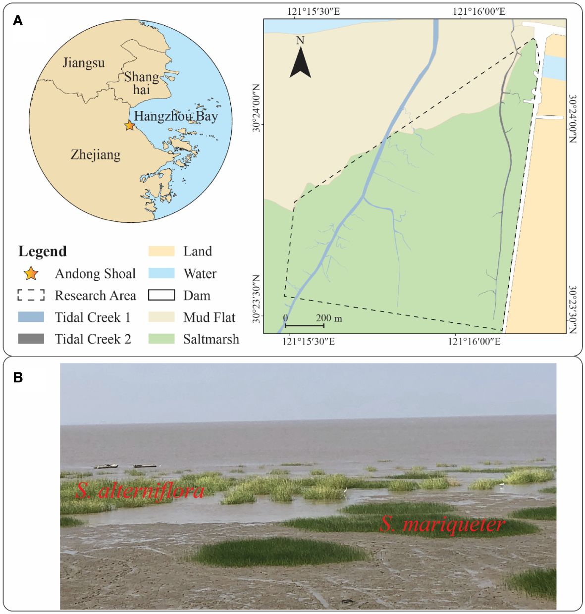
Figure 1 Research area map and plant photos: (A) Research area map with unmodified vector data provided by the National Geomatics Centre of China; (B) Plant photos of S. alterniflora and S. mariqueter.
The upper portion of the mudflat in this region is colonized by saltmarsh plants, with two predominant species (Figure 1B): the native species S. mariqueter and the exotic species S. alterniflora. These species demonstrate zonation patterns, with interspecific competition linked to ground elevation. S. alterniflora typically occupies the upper saltmarsh, extending into the pioneer zone dominated by S. Mariqueter (Huang et al., 2020). Both species’ plant patches can be found in the pioneer zone. S. alterniflora exhibits higher aboveground and belowground biomass compared to S. mariqueter due to differences in primary production (Cai et al., 2023). In our study, UAV-based LiDAR scanned the pioneer zone of a saltmarsh in Andong Shoal (Figure 1A) to unveil the canopy morphological characteristics of the native and exotic species’ plant patches. Two tidal creeks were observed within the LiDAR scanning range.
2.2 Data acquisition and pre-processing
A DJI M300 RTK UAV equipped with a DJI ZENMUSE L1 sensor (Figure 2) was employed to capture optical images and LiDAR data across the research area. To mitigate the adverse effects of surface water, air humidity, and rain on laser data collection, the aerial survey was conducted judiciously at a flight altitude of 120 m during low tide on July 31, 2021. The survey utilized a non-repeating scanning mode, with the UAV flying straight towards the vertical coastline at a yaw angle of ±90°, pitch angle of 0°/180°, and roll angle of -90° (Supplementary Figure 2). The LiDAR sensor had a Field of View (FOV) of 70.4° × 77.2°, while the camera had a FOV of 95°. Although the L1 sensor could support up to three returns, typically only one return was detected for most saltmarsh areas, with a few areas of S. mariqueter showing a second return. Ground returns were virtually non-existent under dense vegetation.
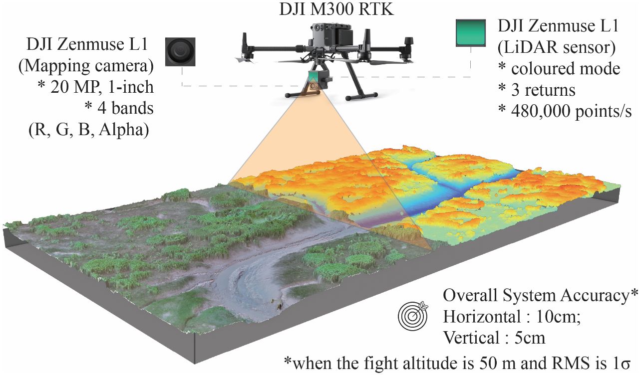
Figure 2 Schematic and key parameters of the imagery and point cloud data collected by the DJI Zenmuse L1.
The optical images and LiDAR data were reconstructed using DJI Terra software into GeoTIFF and LAS format datasets. Subsequently, LIDAR360 software was utilized to conduct multi-faceted preprocessing on the LiDAR point cloud through an optimized workflow. The preprocessing began with the application of the Noise Filter tool, employing refined parameters of 30 neighbor points and 3 standard deviations to eliminate sporadic noise points above the vegetation and surface. Following this, anomalously low pseudo ground points were separated using the Classify Low Points tool, with optimized parameters of 1 minimum point, 5 search radius, and 0.5 maximum height difference. Finally, a high-resolution Digital Surface Model (DSM) was generated based on the preprocessed point clouds, providing an accurate surface model representing vegetation and ground surfaces (Guo et al., 2023).
2.3 Data analysis
The data analyses primarily focused on planimetric morphology extraction and three-dimensional canopy feature analysis (Figure 3). Patch morphology was extracted through threshold segmentation with color information, and elliptic parameters were calculated using analytic geometry. Vertical canopy characteristics included canopy height and internal height variation, which were determined by combining spatial statistics with elevations in the LiDAR point cloud.
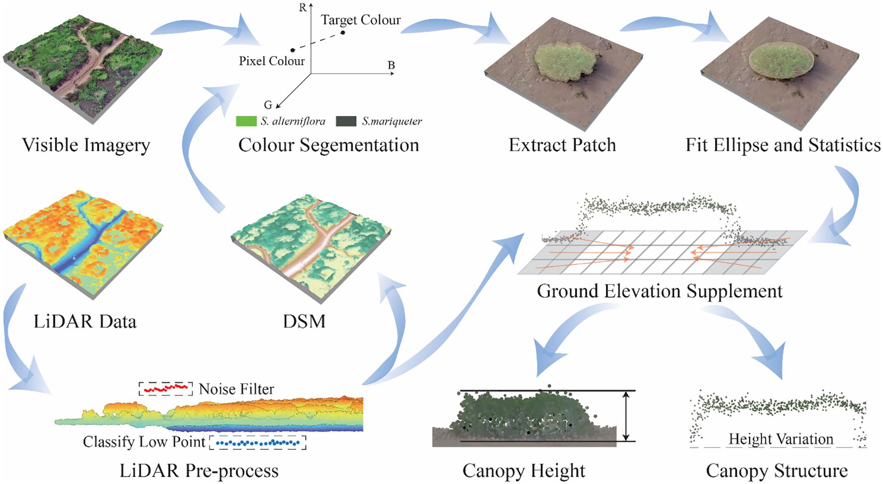
Figure 3 Research flow chart.
2.3.1 Vegetation extraction and accuracy assessment
The primary land cover types within the study area are vegetation and mudflat, which exhibit significant differences in color information. Additionally, the two dominant species, S. alterniflora and S. mariqueter, display noticeable bright and dark green color contrasts. To extract plant information, we employed the Mahalanobis distance approach from computer graphics for color image processing (Gonzalez and Woods, 2017).
As elevations generally decrease from landward to seaward and vegetation habitats are limited to certain elevation ranges, DSM thresholding was initially applied to narrow the focus area to vegetated zones, using a threshold of 1.50 m. Subsequently, the reconstructed optical image was leveraged to calculate Mahalanobis distances (Equation 1) from specified color signatures for each pixel:
Where μ and φ denote the RGB components of the pixel and target color, and C is the covariance matrix for samples within the color range. Manual threshold segmentation was used to confirm the color extraction threshold. Representative color of RGB (0, 255, 0) was used for S. alterniflora with respective segmentation thresholds of 377.6593, whereas RGB (70, 80, 70) was used for S. mariqueter with respective segmentation thresholds of 6.3991.
In order to test the accuracy of plant species classification based on threshold segmentation methods, an error matrix approach was employed to assess the accuracy of vegetation extraction (Deng et al., 2010). Due to the availability of remote sensing image resources, a 3-m multispectral satellite PlanetScope image produced on July 29, 2021 turned to be the only choice considering survey date and cloud cover. We visually classified 30 S. alterniflora samples and 20 S. mariqueter samples from the PlanetScope image (see the details from Supplementary Figure 3), then the accuracy validation of vegetation classification of the UAV-based orthoimages was done by the error matrix approach. The accuracy rates for S. alterniflora and S. mariqueter were determined to be 81.27% and 85.91%, respectively.
2.3.2 Planimetric characteristics of patch canopies
Since the research topic centered on the canopy characteristics of plant patches, patch information was extracted separately and further described in terms of their number and size. A series of semi-automated patch extraction steps were devised to determine the number, area, and equivalent axes of the patches. Ellipse fitting was employed as an intermediate step to illustrate the patch features. Additionally, the main axes were extracted synchronously in this section as the basis for the height variation characteristics. Following the initial extraction, the vegetation raster data were converted to vector format. Subsequently, manual screening, editing, and correction processes were carried out to derive final vector layers representing S. alterniflora and S. mariqueter patches.
Both S. alterniflora and S. mariqueter patches displayed near-elliptical shapes, which were discernible in the remote sensing image and confirmed by field measurements. Previous studies have also shown that ellipsoidal shapes are effective approximations for plant outlines (Russell et al., 1990). Therefore, ellipses were chosen as the geometric construct to characterize planimetric patch morphology. Based on mathematical representations of ellipses from analytic geometry, the general equation for an ellipse in matrix form (Equation 2) is:
Where a to f are coefficients, χ and γ are coordinates, and the ellipse equation has the constraint b2 – 4ac< 0. Not all points on plant patch outlines can perfectly fit the ellipse equation, so estimation with constraints was needed using Least Squares Minimization (LSM) (Halır and Flusser, 1998; Qiu, 2015).
After obtaining the best-fit ellipse equation, each ellipse was visualized in ArcGIS. Size characteristics, such as perimeter and area, were calculated using the Geometry Attributes tool in ArcGIS. Axial characteristics, including major and minor lengths, were also quantified within ArcGIS. Eccentricity, which represents the degree of elliptical shape, could be computed using the semi-lengths of the major and minor axes (Qiu, 2015).
Statistics were compiled for each patch in relation to environmental factors. Regarding elevations, the research analyzed and visualized the number and area of patches across elevation gradients. For distances from tidal creeks, the tidal creeks and corresponding catchments were manually extracted and calculated. Within each catchment, distances from patches to tidal creeks were determined using the Near tool in ArcGIS. Finally, the number and area of patches within each distance gradient were tallied.
2.3.3 Vertical characteristics of patch canopies
2.3.3.1 Ground elevations supplement based on spatial statistics model
Due to the lack of ground returns under dense plant cover, a workflow was established to reconstruct inner-patch ground elevation. Since the mudflat near plant patches had connectivity to the inner-patch ground with abundant elevation information, their elevations were considered to complete the inner-patch ground elevations. However, the complex and biased nature of the discrete point cloud made it challenging to calculate in practice and control the accuracy of infill. Therefore, grids were established to simplify calculation. During the calculation, it was observed that the patch sizes varied widely, making it difficult to standardize to a uniform area or number. Hence, the spatial statistics method was utilized to determine the grid size.
To overcome this obstacle, spatial autocorrelation principles were integrated to delineate grid cells (Dale and Fortin, 2014). The neighbor parameter from spatial autocorrelation was utilized to determine the point counts per grid cell and the overall number of grids. Given the total number of grids, the coefficient of determination (R2) and Root Mean Square Error (RMSE) of mean grid elevation representing points were evaluated for various row and column combinations. The configuration that resulted in the maximum R2 was selected as the optimal grid segmentation (ten Harkel et al., 2020). Based on the optimized plant patch grids, the patch buffer was generated and divided into a ring of mudflat cells. The mean ground elevation was calculated for each grid cell of the mudflat. The process of calculation was shown in Supplementary Figure 4. Trend analysis (Equation 3) and LSM were then employed to estimate the lack of ground elevations under the patch canopy using the ground elevations of gridded mudflat cells:
Where δ0 is the intercept, δ1 and δ2 are coefficients, χ and γ are the center coordinates of each grid. Notably, the original plant patch vector was utilized for filtering at the stage to ensure the resultant gridded elevations could characterize the ground surface underlying the plant canopy.
Concurrent Real-Time Kinematic (RTK) measurements within canopies were utilized for post-processing validation of the calculated ground elevations. The distances between RTK points were determined based on the size of the patches. For S. alterniflora, 7 patches were surveyed using RTK, with 3-6 field points collected per patch, totaling 31 ground points. For S. mariqueter, 6 patches were surveyed using RTK, with 2-4 field points collected per patch, totaling 18 ground points. The accuracy of ground elevations was assessed using two datasets: the elevations collected by RTK and the estimated ground elevations. For S. alterniflora patches, the RMSE was 0.14 m based on the elevation measured by RTK. For S. mariqueter patches, the RMSE was 0.09 m. These results suggested that the spatial statistics model can generate suitable ground elevations supplementation.
2.3.3.2 Plant canopy height and statistics
The passage of Typhoon In-Fa across Hangzhou Bay on July 26, 2021 caused significant disturbance to patches, resulting in the collapse of some parts of the canopy. During the investigation, it was found that there were many bended S. mariqueter patches, which were removed in subsequent research for canopy height study. After removing these highly disturbed patches, the plant canopy height was computed by determining the maximum difference between the canopy surface point elevations and the estimated ground elevation. For S. mariqueter patches located at the tidal creek bank with steep slope steepness, manual extraction of canopy height was conducted for these three patches as an alternative approach. Following the finalization of canopy height data, descriptive statistics, including the maximum, minimum, mean, standard deviation and frequency histograms were compiled using Python.
2.3.3.3 Plant height variation along axes and statistics
It was critical to identify internal canopy features that could indicate the biogeomorphological processes. Fairy circles, which show a double-arch pattern along axes, are an essential criterion for determining patch evolution and ecological resilience (Zhao et al., 2021).
Plant heights were obtained by subtracting the ground elevation from the plant surface elevation without interference from the intermediate point cloud. A multi-step procedure was devised to profile canopy morphology:
STEP 1 - Plant point elevations were extracted along the major and minor axial vectors buffered by one grid length, and the estimated ground elevation was subtracted to derive plant point heights along each axis, denoted as Y;
STEP 2 - Patch centers served as the coordinate origin. Longitudinal points were sorted by increasing longitude, normalized from [-1,0) when less than the center to (0,1] when greater, collectively denoted as X;
STEP 3 - To standardize the broad height ranges, plant heights of each canopy were normalized by the canopy height, scaling Y to (0,1];
STEP 4 - Plant heights were plotted in scatter figure. Characteristic types of height elevation were summarized, and appropriate functions were fitted for each morphological category.
Through integrating LiDAR data analysis and field observations, two types of predominant canopy vertical morphology were found within the study area: The first type exhibited single-arch pattern, and the second one displayed double-arch pattern. The fitting function of single-arch pattern (Equation 4) was:
The fitting function of double-arch pattern (Equation 5) was:
Where x is the data of X, y is the data of Y, and a1, a2, β0, β1, β2, ω are coefficients. Following the derivation of fitting functions, the morphological categories were visually characterized through spatial mapping of patches exhibiting representative structural attributes, scatter plots overlaying the height data and fitted curves.
2.3.4 Vertical feature accuracy verification
To demonstrate the validity of estimation methodology, the study utilized the Riegl VUX-1 LiDAR sensor, RTK, and plant sample to survey plant patches within the study area. The experimental design and the accuracy of methodology were shown in Figure 4.
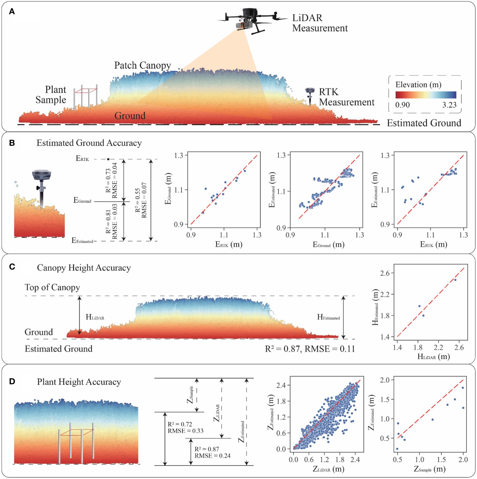
Figure 4 Accuracy verification of vertical features: (A) validation approach diagram combining LiDAR, RTK and plant sample survey; (B) ground elevation estimation accuracy; (C) patch canopy height calculation accuracy; (D) gridded plant height estimation accuracy.
Previous studies had used the DJI L1 sensor to investigate saltmarsh in similar bay environments, with the average RMSE in measuring saltmarshes was approximately 0.10 m (Curcio et al., 2022). Both DJI L1 and Riegl VUX-1are high precision LiDAR sensors in the elevation measurements. RTK, which could be used as a validation dataset, is a high precision tool in measuring elevations. Plant samples are field-based measurements that could also become a useful validation methodology.
The study utilized a hexacopter UAV equipped with a Riegl VUX-1 LiDAR sensor to scan the saltmarsh at a flight altitude of 20 m, with a roll angle of ±180° and a pitch angle of ±5°. Three S. alterniflora patches were effectively scanned, with the maximum number of returns from the vegetation being 4. For each patch, five 50 cm × 50 cm plant samples were collected along the main axis, and the height of the tallest plant within each sample was measured using a tape measure. Concurrently, 30 RTK field points were collected during the plant sample collection process. The distance between each ground point was determined based on the size of the patch, ensuring it was as even as possible within the same patch.
To evaluate ground elevation accuracy (Figure 4B), the difference in measured elevation between the RTK (ERTK) and LiDAR sensors (EGround) was initially verified. Comparing the accuracy of both sensors revealed an RMSE of 0.04 m. Subsequently, the study re-estimated the ground elevation of patches (EEstimated) using trend analysis with the ground elevations of the mudflat. The original patch ground elevations and the estimated elevations were used for accuracy validation, resulting in an RMSE value of 0.03 m. Furthermore, accuracy validation was performed using the RTK data and the estimated ground point cloud, indicating an RMSE of 0.08 m. Combining these three sets of data showed that the estimated ground elevations were highly accurate when compared to the original point cloud elevations. Additionally, the accuracy of the estimated ground elevation when compared to the RTK data was deemed acceptable, considering the systematic errors of the RTK and LiDAR sensors.
For patch canopy height accuracy (Figure 4C), the canopy heights in traditional method (HLiDAR) were obtained by subtracting ground elevations from top elevations of canopy point cloud, and the canopy heights in estimated method (HEstimated) used the maximum estimated gridded plant heights. The accuracy of both methods was evaluated, resulting in an RMSE of 0.11 m. For gridded plant height accuracy (Figure 4D), the plant heights within each grid were validated using the traditional method (ZLiDAR) and the estimated method (ZEstimated), with a verified accuracy of an RMSE of 0.24 m. Additionally, plant heights with each sample were validated using plant sample survey data (ZSample), with an RMSE of 0.33 m. This research employed three different methods of vertical data collection and designed six accuracy tests to confirm the validity of the analysis in the absence of ground returns within plant patches. Overall, the estimated approach demonstrated a certain degree of reliability by passing the accuracy tests.
3 Results
3.1 Patch planimetric morphology
For S. alterniflora, a total of 748 patches were scanned by LiDAR, with one example and histograms shown in Figure 5. These patches ranged from 8.17 m to 44.66 m in perimeter, with an average of 15.47 ± 5.24 m, and from 5.13 m2 to 149.39 m2 in area, with an average of 19.62 ± 15.11 m2 (Figure 5B). The distribution of perimeter and area followed a unimodal histogram pattern with leptokurtic and positively skewed modes, indicating a dominance of small patches. In terms of eccentricity, the patches exhibited a range of 0.18 to 0.96, with a mean of 0.68 ± 0.15 (Figure 5C). The distribution of eccentricity showed a unimodal, leptokurtic, and negatively skewed histogram pattern, suggesting that oblate patches were predominant. Regarding axial length, the major axial length varied within a range of 2.74 m to 18.80 m, with an average of 5.80 ± 2.14 m, while the minor axial length ranged from 1.74 m to 11.89 m, with an average of 3.93 ± 1.31 m (Figure 5D). The unimodal distribution histograms of both major and minor axes were leptokurtic and positively skewed, indicating that major and minor axes were predominantly characterized by relatively short lengths, less than 5.80 m for the major axis and 3.93 m for the minor axis.
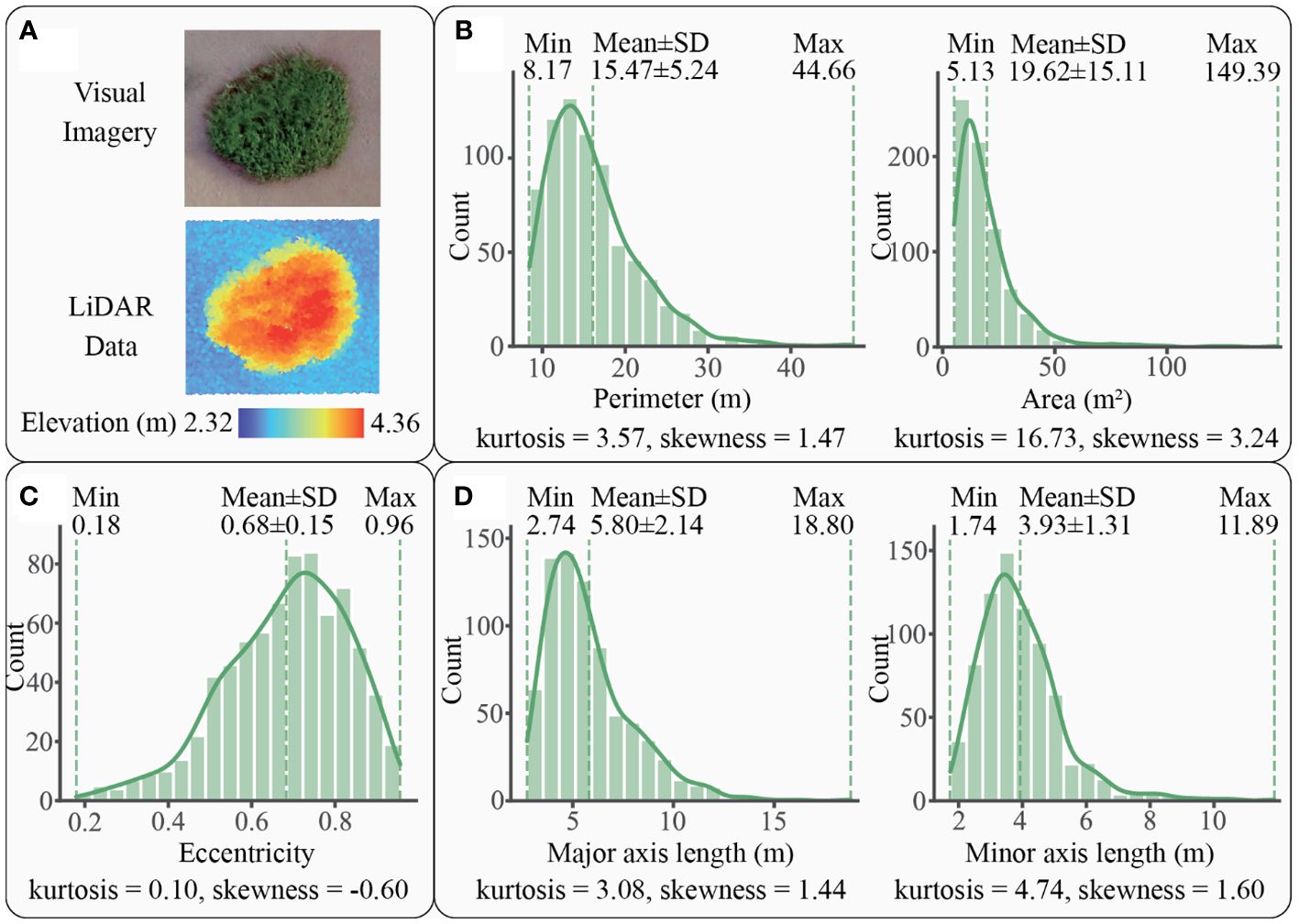
Figure 5 A patch example and the statistics graphs of S. alterniflora patches: (A) an example of patch imagery and elevation data scanned by LiDAR, (B) patch size of S. alterniflora with kernel density curve in solid line, (C) patch shape of S. alterniflora with kernel density curve in solid line, (D) axial lengths of S. alterniflora patch with kernel density curve in solid line.
For S. mariqueter, a total of 128 patches were detected by LiDAR. An example and histograms of these patches were displayed in Figure 6. The patch perimeters varied within a range of 0.49 m to 82.53 m, with an average of 26.66 ± 13.96 m, while the area ranged from 0.02 m2 to 357.80 m2, with an average of 61.62 ± 62.64 m2 (Figure 6B). The distribution of perimeter and area followed a unimodal histogram pattern with leptokurtic and positively skewed modes, indicating the domination of small patches. Regarding eccentricity, the patches exhibited a range of 0.25 to 0.99, with a mean of 0.76 ± 0.15 (Figure 6C). The distribution of eccentricity showed a unimodal, leptokurtic, and negatively skewed histogram pattern, suggesting that oblate patches were the majority. In terms of axial lengths, the patches ranged from 0.18 m to 39.04 m in major axis, with an average of 10.46 ± 5.72 m, and from 0.12 m to 18.87 m in minor axis, with an average of 6.11 ± 3.51 m (Figure 6D). The distribution of major and minor axes followed a unimodal histogram pattern with leptokurtic and positively skewed modes, indicating a dominance of relatively short lengths, less than 10.46 m for the major axis and 6.11 m for the minor axis.
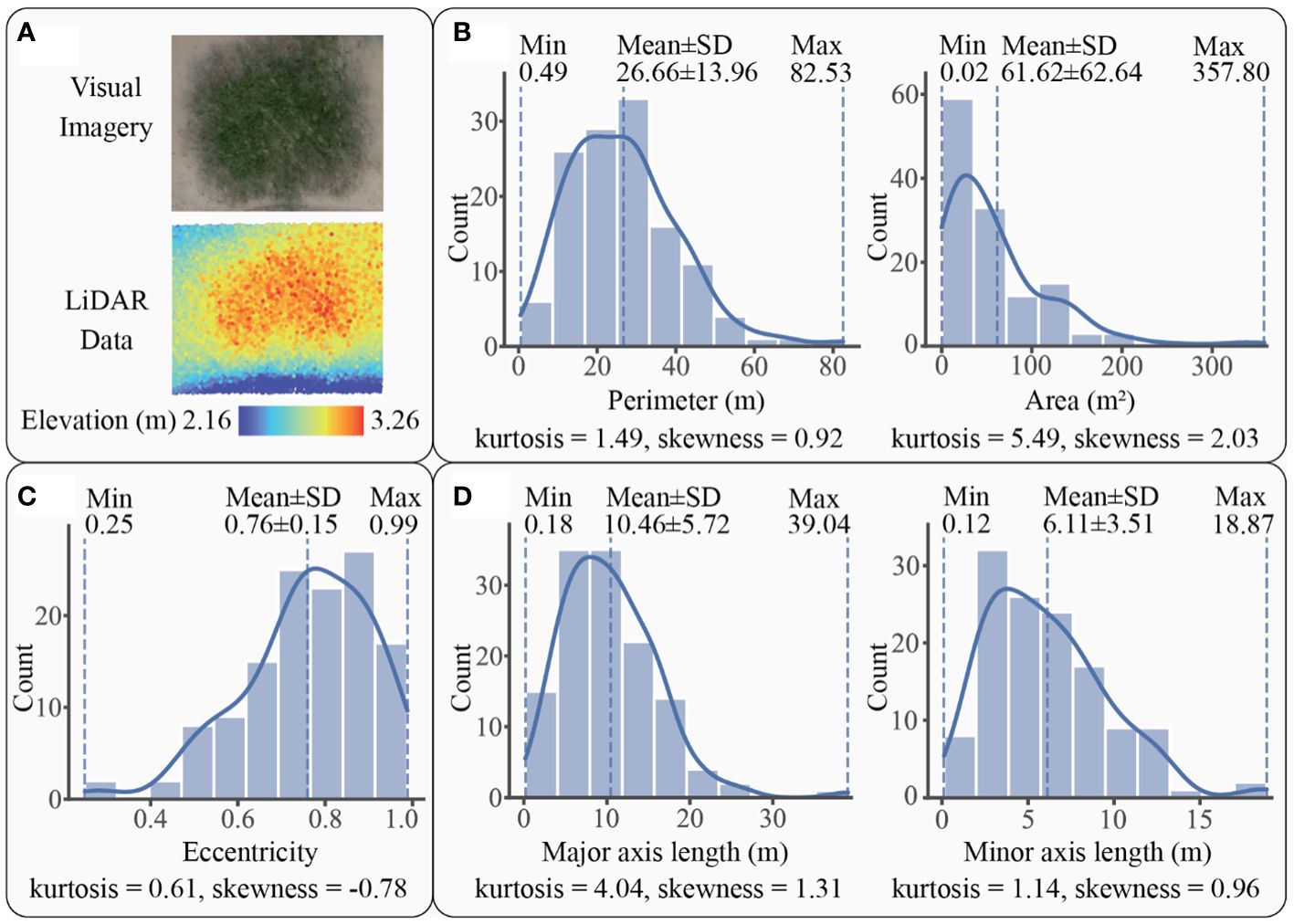
Figure 6 A patch example and the statistics graphs of S. mariqueter patches: (A) an example of patch imagery and elevation data scanned by LiDAR, (B) patch size of S. mariqueter with kernel density curve in solid line, (C) patch shape of S. mariqueter with kernel density curve in solid line, (D) axial lengths of S. mariqueter patch with kernel density curve in solid line.
Perimeter, area, eccentricity, and axial lengths of both species conformed to unimodal distributions with positive kurtosis, indicating that the distributions were peaked and relatively sharp. Additionally, the size and axial length distributions had positive skewness, indicating that they were skewed towards smaller values, while the shape distribution was negatively skewed, suggesting a dominance of oblate shapes. This pattern indicated that both S. alterniflora and S. mariqueter were dominated by small and oblate patches with short axes. However, the averages of perimeter, area, eccentricity, and axial length of S. mariqueter were much larger than those of S. alterniflora, suggesting that S. mariqueter possesses larger size, more oblate shapes, and longer axial lengths.
3.2 Plant canopy characteristics revealed by LiDAR
3.2.1 The canopy height of the two saltmarsh species
Canopy height is defined as the maximum plant height within a patch, corresponding to the maximum value of plant elevation minus ground elevation. It serves as a direct trait within the patches from a vertical perspective, which is a key parameter in biogeomorphology. Due to the bending of many S. mariqueter shoots caused by Typhoon In-Fa prior to the LiDAR measurement, only 40 S. mariqueter patches were practically calculated for canopy height. In contrast, S. alterniflora was rigid and stiff, so their canopies were nearly not affected by the typhoon event. Therefore, 748 S. alterniflora patches were used for the canopy height calculation, following the workflow described in Section 2.3.3. The statistical results of patch canopy height calculated by the LiDAR point cloud data are presented in Figure 7.
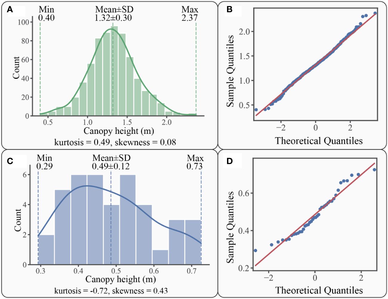
Figure 7 Statistics graphs for patch canopy height: (A) canopy height of S. alterniflora patches distribution histogram with kernel density curve in solid line; (B) Q-Q plot of S. alterniflora patches canopy height; (C) canopy height of S. mariqueter patches distribution histogram with kernel density curve in solid line; (D) Q-Q plot of S. mariqueter patches canopy height.
For S. alterniflora, the canopy heights of those patches varied within a range of 0.40 m to 2.37 m, with an average of 1.32 ± 0.30 m (Figure 7A). Most canopy heights of those patches (75%) ranged from 0.99 m to 1.66 m. The canopy height distribution was leptokurtic (kurtosis = 0.49), indicating that 70.67% of patches were within a range of 1.02-1.62 m in canopy height. The unimodal distribution histogram had a positive skewness (skewness = 0.08), which indicated that 51.56% of patch canopy heights were less than the average of 1.32 m. However, the percentage of patches larger than the mean height of 1.32 m was also considerable, reaching 48.44%. The Kolmogorov-Smirnov and Q-Q plot (Figure 7B) tests indicated that the canopy height of S. alterniflora patches followed a normal distribution (p-value=0.59).
For S. mariqueter, the canopy heights varied within the range of 0.29 m to 0.73 m, with an average of 0.49 ± 0.12 m (Figure 7C). 75% of the patches ranged from 0.35 m to 0.66 m. The distribution was platykurtic (kurtosis = -0.72), indicating that most patches (67.5%) were within a range of 0.37-0.61 m in canopy height. The histogram was positively skewed (skewness = 0.43), suggesting that more than half of patch canopy heights (57.50%) were less than the average of 0.49 m. However, it was worth considering that 42.50% of patches had canopy heights larger than the mean value of 0.49 m. The Kolmogorov-Smirnov and Q-Q plot (Figure 7D) tests indicated that the canopy height of S. mariqueter patches also followed a normal distribution (p-value=0.90).
Both S. alterniflora and S. mariqueter patches exhibited a wide range of canopy heights without obvious dominance. The distribution of canopy height followed a unimodal histogram pattern with positive skewness. However, there were some differences between the two species. S. alterniflora patches generally had a higher canopy height than S. mariqueter patches, approximately 2.72 times the latter. Moreover, the distribution of S. alterniflora patches was leptokurtic, while that of S. mariqueter patches was platykurtic. These different kurtosis patterns indicated that S. mariqueter had a relatively similar pattern for each height interval, while S. alterniflora had a more concentrated pattern in terms of canopy height distribution.
3.2.2 Canopy height variation along main axes
To reveal the difference in canopy morphology for the two species, the surface elevation data obtained by LiDAR were converted into canopy height variation along main axes at an individual patch scale. The datasets of canopy characteristics based on canopy height variation are displayed in Figure 8.
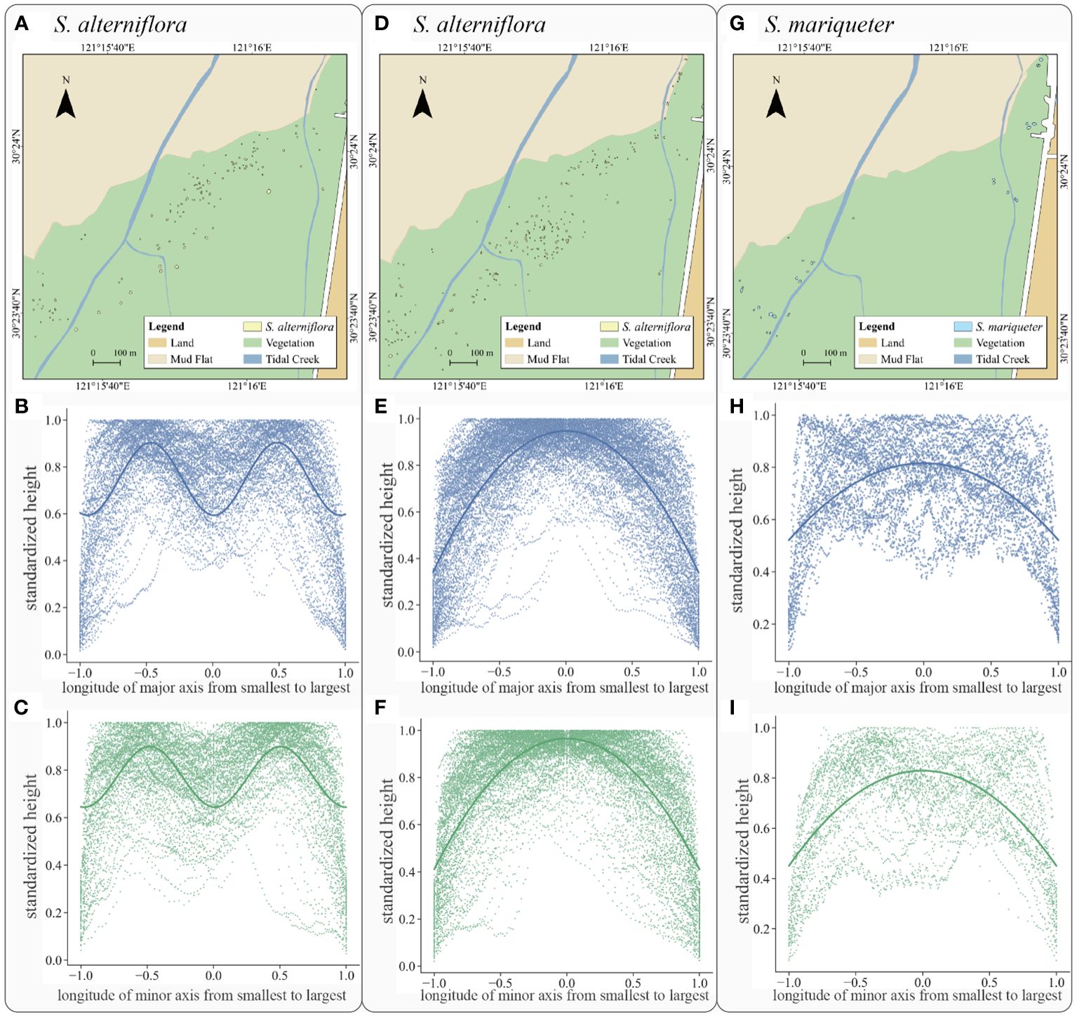
Figure 8 Plant patch type, distribution and fitting curve: (A) the spatial distribution of S. alterniflora with double-arch shape, (B) the major axis fitting curve of S. alterniflora with double-arch shape, (C) the minor axis fitting curve of S. alterniflora with double-arch shape, (D) the spatial distribution of S. alterniflora with single-arch shape, (E) the major axis fitting curve of S. alterniflora with single-arch shape, (F) the minor axis fitting curve of S. alterniflora with single-arch shape, (G) the spatial distribution of S. mariqueter, (H) the major axis fitting curve of S. mariqueter, (I) the minor axis fitting curve of S. mariqueter.
For S. alterniflora patches, there were two types of canopy characteristic: the first group exhibited a double-arch distribution along the main axes, whilst the second group showed a single-arch shape and the rest of those patches had uniform heights.
The S. alterniflora patches in double-arch shape included 122 patches (Figure 8A). After regression analyses (solid line in Figure 8B of major axis and Figure 8C of minor axis), the plant canopy height variation along the major and minor axes showed a low value at x of 0 and 1, but peaks at x of -0.5 and 0.5. This pattern indicated that tall plants occurred around the place in half of patch radius, while relatively short plants appeared either on the edge or in the center. The optimal fitting equations of canopy height variations were summarized by Equations 6, 7, Equation 6 for the variation along the major axis, while Equation 7 for the variations along the minor axis:
where y is the normalized height and x is the normalized distance from the center of the patch, both within the range of [-1,1].
The second type emerged within 218 S. alterniflora patches (Figure 8D). There was no obvious difference in terms of the spatial distribution of those two types of patches. After regression analyses (solid line in Figure 8E of major axis and Figure 8F of minor axis), the plant canopy height variation along the major and minor axes showed a low value at x of -1 and 1, but a peak at the center of the patch. This pattern indicated that tall plants appeared in the center while plant height decreased with the increasing distance from the center. The optimal curve equations canopy height variations were summarized by Equations 8, 9, Equation 8 for the variation along the major axis, while Equation 9 for the variations along the minor axis:
Between those two types of S. alterniflora patches, the second type had approximately twice as many patches as the first type. For the plant heights, the tallest plant height corresponding to the second type was greater than that of the first type, but the relative height at the edges of the second type was lower than that of the first type. The appearance of different height variations of the same species was likely related to different patch growth stages.
For S. mariqueter, 33 patches followed the same type (Figure 8G): a single-arch distribution along the main axes, and the other 7 patches showed no obvious variations. After regression analyses (solid line in Figure 8H of major axis and Figure 8I of minor axis), the plant canopy height variation along the major and minor axes peaked at x = 0 but showed a low value at x = -1 and 1. This pattern indicated the presence of tall plants in the center, while the plant height decreased with increasing distance from the center. The optimal curve fitting equations for canopy height variations were represented by Equations 10, 11, Equation 10 for the variation along the major axis, while Equation 11 for the variations along the minor axis:
The canopy height variations along main axes of S. alterniflora and S. mariqueter patches exhibited a similar pattern following a single-arch shape. Most of S. mariqueter patches (82.50%) were in single-arch shape whilst only 29.14% of S. alterniflora patches were found to follow this pattern. For the single-arch pattern of height variations, comparing the parabolic equations of the two species, S. alterniflora had larger intercepts and smaller quadratic coefficients on both the major and minor axes. The double-arch pattern of height variations of S. alterniflora plant patches suggested that LiDAR successfully captured the developing fairy circle from the vertical dimension. For height variations of plant patches of the two species, the relative height of the S. alterniflora patch center was much higher than that of S. mariqueter patches, and the height of the edge decreased more rapidly.
3.3 Patch characters within environmental gradients
There were two environmental gradients in the study area: elevation and distance from tidal creeks. Patches responded differently to environmental gradients. Hence, the relationships between the patch properties and the environment were shown in Figure 9.
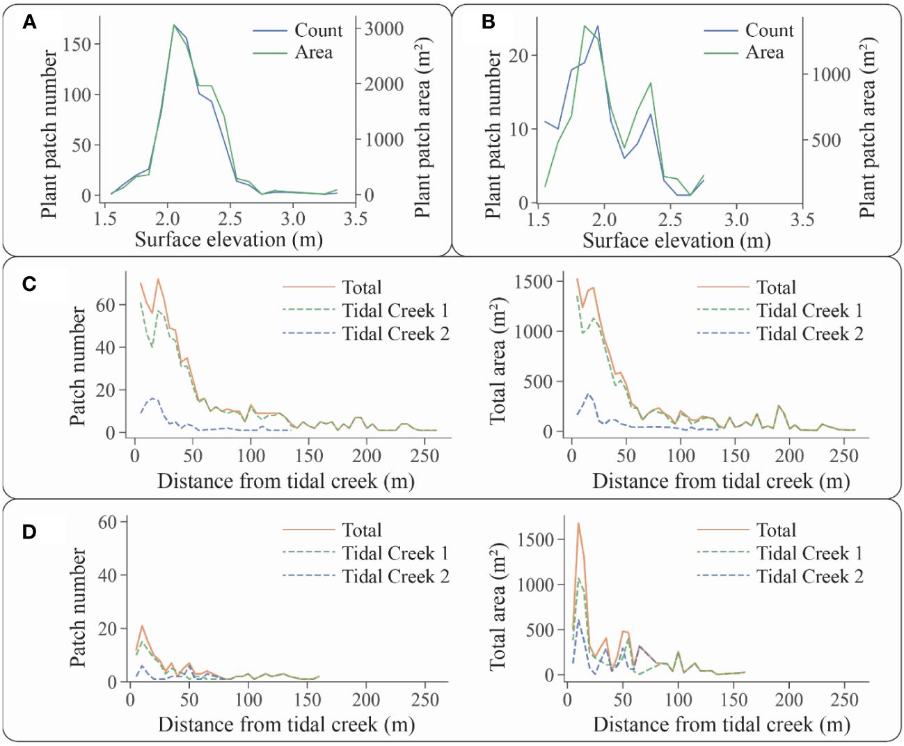
Figure 9 Relationships between the number and area of plant patches and environmental factors: (A) relationship between the number and area of S. alterniflora patches and surface elevation; (B) relationship between the number and area of S. mariqueter patches and surface elevation; (C) relationship between the number and area of S. alterniflora patches and their distance from tidal creeks; and (D) relationship between the number and area of S. mariqueter patches and their distance from tidal creeks.
For S. alterniflora patches, they were distributed at surface elevations ranging from 1.55 m to 3.35 m, with an average of 2.16 ± 0.22 m (Figure 9A). When surface elevations were less than 2.00 m, the severe environmental conditions of saltmarsh fronts were unsuitable for S. alterniflora colonization and growth. As surface elevations exceeded 2.25 m, S. alterniflora gradually formed a continuous distribution without the formation of distinct patches. The elevation distribution of S. alterniflora patches indicated that for the optimum elevation range is 2.00 m to 2.25 m for the growth of pioneer S. alterniflora in the research area.
For S. mariqueter patches, their distribution varied in the range of 1.55 m to 2.75 m in surface elevations, with an average of 1.96 ± 0.28 m (Figure 9B). There were two peaks of patch distribution at the surface elevations of 1.85-2.00 m and 2.25-2.40 m, whereas a corresponding valley appeared at the surface elevation of 2.00-2.25 m. S. mariqueter began to establish and propagate at an elevation of 1.60 m. Our study revealed that on the front area of the saltmarshes, the number of patches was large, but the patch area was small, corresponding to the smaller patches colonizing lower mudflats. On the upper elevations of saltmarshes, such as 2.25-2.40 m, the number of patches decreased, but the patch area was large, corresponding to less patches with a larger area at higher elevations. When the surface elevation exceeded 2.50 m, S. mariqueter became meadow. The elevation distribution of S. mariqueter patches indicated the optimal growth elevations are approximate 1.95 m and 2.35 m for the pioneer S. mariqueter in the research area.
Consequently, surface elevations played a crucial role as stress gradients affecting species distribution. In eastern Andong Shoal, both S. alterniflora and S. mariqueter not only exhibited fewer patches at low elevations, but also fewer patches at high elevations due to conversion to meadows. However, the responses of the two species to elevation gradients were different. S. mariqueter, being the pioneer species in the shoal, colonized the mudflat with an average elevation of 1.96 m, which was lower than that of S. alterniflora at 2.16 m. As an invasive species, S. alterniflora possessed a competitive advantage, leading to the peak of S. alterniflora patch numbers and the valley of S. mariqueter patch numbers at a surface elevation of 2.05 m. Unlike the uniform-size patches of S. alterniflora, the size distribution of S. mariqueter varied, with more small patches near the seaward and fewer large patches in the landward areas.
In terms of the relationship between tidal creeks and S. alterniflora patches, those patches were distributed between 0.93 m and 256.56 m from tidal creeks, with an average distance of 51.04 ± 53.79 m (Figure 9C). Approximately half of the patches (51.47%) located within the range of 10.00 to 50.00 m in distance from tidal creek. When the distances were less than 10.00 m, the significant geomorphological change from platforms to tidal creeks was unsuitable for S. alterniflora growth. When the distance exceeded 50.00 m, the S. alterniflora patches merged into continuous distribution. Regarding the perpendicular changes from tidal creeks, plant patches exhibited similar variations in number and area for both creeks, suggesting an influence of tidal creeks on patch distribution.
In terms of the relationship between tidal creeks and S. mariqueter patches, they located in distance from tidal creeks ranging from 2.05 to 158.80 m, with an average distance of 40.20 ± 40.97 m (Figure 9D). Approximately half of the patches (50.78%) were distributed between 5.00 m and 35.00 m from tidal creeks. When the distances were less than 5.00 m, the tidal creek bank was unsuitable for S. mariqueter growth. When the distances exceeded 35.00 m, both the patch number and area decreased, leading to a transition into continuous distribution. Regarding the perpendicular changes from tidal creeks, plant patches exhibited similar variations in number and area for both creeks, suggesting an influence of tidal creeks on plant patch distribution.
We summarized the relationships between single-arch and double-arch S. alterniflora patches and environmental factors in Supplementary Figure 5. There were no significant differences in the behavior of single-arch and double-arch patches across gradients of surface elevation and distance from tidal creeks.
4 Discussion
4.1 Advantages of LiDAR in measuring canopy morphology
LiDAR technology has revolutionized ecological sciences by offering precise three-dimensional mapping and quantification of the ecosystems (Eitel et al., 2016). Unlike passive spectral remote sensing instruments limited to surface data, LiDAR provides detailed vertical and internal vegetation structure information, enhancing accuracy and efficiency (Guo et al., 2021). Compared to traditional point-format GNSS measurements, UAV-based LiDAR offers high-density, high-repetition data, along with comprehensive orthographic images for interpretation (Cohen and Héquette, 2020). Our research utilized UAV-based LiDAR to precisely measure the planimetric morphology and vertical trait of plant patches, overcoming the limitations of optical satellite remote sensing. This advancement elevates canopy research from two-dimensional to three-dimensional perspectives.
LiDAR stands out as a promising technology for characterizing vegetation structure, capable of estimating canopy height, internal variation, and surface information beneath canopies (Huylenbroeck et al., 2020; Campbell et al., 2022). Previous studies on UAV-based photogrammetry and LiDAR in saltmarsh environments have highlighted the superiority of UAV-based LiDAR for mapping and modeling canopy height. This technology overcomes limitations of traditional methods like Structure from Motion (SfM), providing improved canopy structural information and opportunities for high-resolution, temporal mapping (Duffy et al., 2021). Three-dimensional LiDAR measurements offer insights into plant-habitat interactions and biological adaptations to environmental stress, facilitating seasonal change assessments and carbon stock estimations (Omasa et al., 2007; Tempest et al., 2015; Pham et al., 2023). In our research, UAV-based LiDAR formed the basis for understanding canopy height and variations along main axes, representing a significant step towards comprehending the three-dimensional structure of saltmarsh patches, particularly vertical variations. This ongoing research on canopy structures lays groundwork for future studies on coastal ecological structures. However, challenges remain in applying UAV-based LiDAR to coastal saltmarsh vegetation research. Dense canopies, like those of S. alterniflora, pose obstacles to LiDAR detection due to limited laser signal penetration, leading to a lack of internal structure information.
This study utilized UAV-based LiDAR to investigate the small-scale canopy parameters of coastal saltmarshes. A significant finding was the identification of double-arch shaped S. alterniflora patches, suggesting the presence of developing fairy circles within the S. alterniflora population (Figures 8A–C). Unlike previous UAV-based optical remote sensing studies, which only detected already-formed fairy circles, our approach using LiDAR allowed for the detection of developing fairy circles based on connectivity clustering and global geometric features of clusters. Since all the developing fairy circles did not exhibit concentric rings, this implies that sulfide inhibition of vegetation growth may be the mechanism driving the formation of pixie rings in Andong Shoal, Hangzhou Bay. However, this requires further detailed biogeochemical studies in the future (Zhao et al., 2021). S. alterniflora fairy circles are crucial spatial indicators of vegetation resilience, highlighting a rapid transition to S. alterniflora meadows. By enabling the timely assessment of saltmarsh resilience, UAV-based LiDAR plays a critical role in monitoring and managing these habitats. In contrast, S. mariqueter patches did not exhibit fairy circles (Figures 8G–I), suggesting lower resilience compared to S. alterniflora in the Andong Shoal. Resilience is essential for pioneer species like S. alterniflora to establish populations in the pioneering zone of saltmarshes, potentially contributing to its competitive success in this region (Huang et al., 2020). Additionally, UAV-based LiDAR holds promise for estimating below-ground biomass based on root-shoot ratios, providing valuable insights for assessing saltmarsh carbon sequestration capacity in the future (Kirwan and Mudd, 2012).
Patches of S. alterniflora and S. mariqueter in Chinese saltmarshes exhibit scale-dependent characteristics, leading to variations in their physical environment and ecological functions, such as sediment input and hydrodynamic conditions (Schwarz et al., 2015; Zhao et al., 2019; Dai et al., 2021; Yando et al., 2023). However, retrieving vertical information from the canopy becomes challenging due to significant differences in patch scales. To address this issue, we introduced Moran’s I index of spatial autocorrelation to account for the scale difference. Traditional methods like equal-area or equal-number grid analysis may overlook spatial characteristics in the context of inconsistent patch sizes. Therefore, spatial autocorrelation, a concept from spatial ecology, was employed to tackle the spatial scale problem. Ecologists have used spatial autocorrelation to address spatial issues in ecological research and understand the spatial effects on ecology and the environment, with spatial scale being a key focus (De Knegt et al., 2010; Dale and Fortin, 2014). To address this issue, we implemented a series of data processing methods to compensate for the lack of ground points, and we achieved satisfactory processing accuracy. By integrating spatial ecological statistics, we improved accuracy, achieving an RMSE of 0.08 m in estimated elevation and an RMSE of 0.11 m in canopy height.
A good agreement was found in patch size and height between this study and other studies using classic methods such as field measurement and optical remote sensing images. For the diameter of S. alterniflora patches, it was reported by a previous study using google earth images that most of these patches located in a range of 10 m to 30 m (Zhao et al., 2021), which was close to the perimeter (15.47± 5.24 m) found in this study. A national scale survey of Chinese S. alterniflora saltmarshes through in situ measurement revealed the height of this species of 1.00 m to 2.50 m depending on latitudes (Liu et al., 2016), consistent with our results in Hangzhou Bay. Meanwhile, S. mariqueter saltmarshes mainly appear in Yangtze Estuary and its adjacent area, and the canopy height was found between 42-55 cm in this region (Ma et al., 2003; Liu et al., 2021), close to the heights revealed by UAV-based LiDAR in this study.
4.2 Relationship between patches and environmental factors
Ground elevation plays a crucial role in shaping the spatial distribution of vegetation in the Andong Shoal saltmarsh. In the case of S. alterniflora, patches were scarce at elevations below 2.00 m due to reduced seed survival and growth caused by tidal dynamics. Exceeding inundation led to anaerobic soils, sulfide accumulation, and limited S. alterniflora production (Proffitt et al., 2003; Kirwan et al., 2012; Kulawardhana et al., 2015). Conversely, when elevations surpassed 2.25 m, S. alterniflora patches expanded and connected, forming the dominant community, consistent with previous studies indicating community dominance 2-3 years after invasion (Meng et al., 2020; Yan et al., 2022). As for S. mariqueter, patches were less common at elevations below 1.95 m. This is attributed to S. mariqueter’s shallow-rooted nature, making it less resilient to hydrodynamic erosion at lower elevations (Zhu et al., 2012). Optimal plant growth requires specific windows of opportunity at low elevations, determined by factors such as the duration of inundation and sedimentation dynamics (Yuan et al., 2020). Biomass allocation in S. mariqueter shifts from inflorescence and roots to corms and rhizomes as elevations increase (Sun and Cai, 2001). When elevations exceeded 2.25 m, the plant distribution pattern became continuous.
Our study found that S. alterniflora nearly replaced S. mariqueter at an elevation of 2.05 m (Figures 9A, B). This led to a peak in the presence of S. alterniflora patches and a valley in the presence of S. mariqueter patches at the same elevation. S. alterniflora, being an invasive species, occupies a wider ecological niche and has stronger competitive abilities. Previous studies found that biotic factors play a role in the invasion of S. alterniflora (Meng et al., 2020). Its invasive success can be attributed to factors such as genotypic diversity, greater seed dispersal distance, a larger seed bank, and higher propagule survival rates (Wang et al., 2012; Cui et al., 2020). S. alterniflora possesses developed salt glands and specialized stomata, making it more tolerant to salt and submersion than S. mariqueter under cyclic tidal submergence. Crucially, our research found that the canopy height of S. alterniflora surpassed that of S. mariqueter significantly (Figures 7A, C), securing S. alterniflora’s absolute dominance in light competition between the two species. This advantage has led to patches of S. alterniflora occupying habitats with shorter periods of inundation (higher elevations), which in turn has led to S. mariqueter being forced to migrate seaward to survive in harsher habitats (Figures 9A, B).
In this study, both the number and size of two species plant patches showed a decrease as the distance from tidal creeks increased. However, a peak in number and area was present at the closest point to the tidal creeks in the case of S. alterniflora, whereas in the case of S. mariqueter, the peak was present at a greater distance from the tidal creeks (Figures 9C, D). Previous studies have demonstrated that S. alterniflora exhibits high tolerance to salt and flooding, coupled with its well-developed root system (Fan et al., 2020). As a result, S. alterniflora displays greater adaptability to environments near tidal creeks, facilitating rapid colonization and dominance within the community. Tidal creeks exerted spatially differential physical constraints on its growth, primarily relating to factors like elevation, inundation, and salinity. Unlike Andong Shoal in southern Hangzhou Bay, the biomass of S. mariqueter exhibited a peak at the closest point to the tidal creeks in Chongming Island along the Yangtze River Estuary, as revealed by UAV-LiDAR survey data (Tang et al., 2022). These differences between locations highlight the complexity of the effects of tidal creeks on biological colonization, which are influenced by various factors including hydrology, sedimentation, and ecological processes.
Tidal creeks play a crucial role in the exchange of water, nutrients, and sediment, impacting the growth of saltmarsh vegetation (Tan et al., 2020; Wu et al., 2020). Their influence on patch distribution can be attributed to two main factors. Firstly, the stronger hydrodynamic conditions near tidal creeks may limit vegetation colonization. Conversely, the presence of tidal creeks and hidden microtributaries under vegetation cover could help plants by reducing flooding time and increasing species richness (Zedler et al., 1999; Moffett et al., 2010). Moreover, the low salinity zone near tidal creeks, coupled with well-aerated conditions, creates favorable conditions for marsh plant growth (Zheng et al., 2016). Our study observed a significant concentration of plant patches near tidal creeks (Figures 9C, D), implying that these areas serve not only as important sites for early colonization but also as potential corridors for the seaward expansion of vegetation.
5 Conclusions
This study employed UAV-based LiDAR to capture the three-dimensional morphology of coastal saltmarsh plant patches and their relationship with environmental factors in Andong Shoal, Hangzhou Bay. A new workflow was developed to address missing ground returns and related canopy traits, overcoming the challenge posed by the limited penetration ability of low-cost LiDAR sensors in dense vegetation. Key attributes of plant patches and geomorphology, including area, perimeter, canopy height, elevation, etc., can be reliably extracted from LiDAR data. This workflow establishes LiDAR sensors as a viable option for conducting three-dimensional research on plant patches. S. alterniflora patches exhibited double-arch and single-arch patterns, and the double-arch pattern indicates the patches were developing fairy circles. S. mariqueter patches showed single-arch patterns without the structure of fairy circles. The fairy circles reveal that the invasive species S. alterniflora patches had stronger resilience than S. mariqueter patches. Thus, Using UAV-LIDAR technology to monitor fairy circles of S. alterniflora has the potential to be an important tool in the future for combating S. alterniflora invasions. The study explored the optimal growth range of both species in surface elevation and distance to tidal creeks, indicating that LiDAR could acquire detailed biogeomorphological information on saltmarshes and capture the topographic ecological niches. UAV-LiDAR technology could contribute critical information for ecological evolution and biogeomorphological processes in the pioneer area of saltmarshes from a patch scale to landscape scale.
Data availability statement
The raw data supporting the conclusions of this article will be made available by the authors, without undue reservation.
Author contributions
QH: Writing – original draft, Methodology, Formal analysis. ZG: Writing – review & editing. XW: Writing – review & editing, Software, Data curation. YL: Writing – review & editing, Conceptualization. XX: Writing – review & editing, Resources, Project administration. YC: Writing – review & editing, Supervision, Project administration, Methodology, Funding acquisition, Conceptualization.
Funding
The author(s) declare financial support was received for the research, authorship, and/or publication of this article. This work was funded by the National Key Research and Development (R&D) Program of China (Grant No. 2022YFC3105404), the Zhejiang Provincial Natural Science Foundation of China (Grant No. LDT23D06025D06), and the Zhejiang Provincial Science and Technology Plan (Grant No. 2022R52016).
Acknowledgments
Mr. Minmin Ding and Mr. Ziyan Zhang at the Second Institute of Oceanography, MNR are thanked for their kind technical support in fieldwork. Thanks extended to Natural Resources and Planning Bureau of Hangzhou Bay for providing site access.
Conflict of interest
The authors declare that the research was conducted in the absence of any commercial or financial relationships that could be construed as a potential conflict of interest.
Publisher’s note
All claims expressed in this article are solely those of the authors and do not necessarily represent those of their affiliated organizations, or those of the publisher, the editors and the reviewers. Any product that may be evaluated in this article, or claim that may be made by its manufacturer, is not guaranteed or endorsed by the publisher.
Supplementary material
The Supplementary Material for this article can be found online at: https://www.frontiersin.org/articles/10.3389/fmars.2024.1378687/full#supplementary-material
Supplementary Figure 1 | Fairy circles in saltmarsh (image from Zhao et al., 2021).
Supplementary Figure 2 | Flight trajectories for LiDAR survey by UAV.
Supplementary Figure 3 | The collection of plant sample points based on PlanetScope image.
Supplementary Figure 4 | Processes for estimating patch ground elevation based on mud flat information.
Supplementary Figure 5 | Relationships between the number and area of S. alterniflora patches and environmental factors: (A) relationship between the number and area of single-arch patches and surface elevation; (B) relationship between the number and area of double-arch patches and surface elevation; (C) relationship between the number and area of single-arch patches and their distance from tidal creeks; and (D) relationship between the number and area of double-arch patches and their distance from tidal creeks.
References
Belliard J.-P., Temmerman S., Toffolon M. (2017). Ecogeomorphic relations between marsh surface elevation and vegetation properties in a temperate multi-species salt marsh. Earth Surface Processes Landforms 42, 855–865. doi: 10.1002/esp.4041
Bouma T. J., Temmerman S., van Duren L. A., Martini E., Vandenbruwaene W., Callaghan D. P., et al. (2013). Organism traits determine the strength of scale-dependent bio-geomorphic feedbacks: A flume study on three intertidal plant species. Geomorphology 180, 57–65. doi: 10.1016/j.geomorph.2012.09.005
Bouma T. J., van Duren L. A., Temmerman S., Claverie T., Blanco-Garcia A., Ysebaert T., et al. (2007). Spatial flow and sedimentation patterns within patches of epibenthic structures: Combining field, flume and modelling experiments. Continental Shelf Res. 27, 1020–1045. doi: 10.1016/j.csr.2005.12.019
Cai T., Huang S., Wu J., Zhang Z., Xue C., Chen Y. (2023). Saltmarsh carbon stock changes under combined effects of vegetation succession and reclamation. Ecosyst. Health Sustain 9, 114. doi: 10.34133/ehs.0114
Campbell A. D., Fatoyinbo L., Goldberg L., Lagomasino D. (2022). Global hotspots of salt marsh change and carbon emissions. Nature 612, 701–706. doi: 10.1038/s41586-022-05355-z
Campbell G. S., Norman J. M. (1989). “The description and measurement of plant canopy structure.” in Plant Canopies: Their Growth, Form and Function, ed. Russell G. (Cambridge University Press), p. 1–16.
Chen Y., Chen L., Cai T., Xia X. (2020). Advances in biogeomorphology in coastal wetlands and its application in ecological restoration. Oceanologia Limnologia Sin. 51, 1055–1065. doi: 10.11693/hyhz20200300072
Chen C., Zhang C., Schwarz C., Tian B., Jiang W., Wu W., et al. (2022). Mapping three-dimensional morphological characteristics of tidal salt-marsh channels using UAV structure-from-motion photogrammetry. Geomorphology 407, 108235. doi: 10.1016/j.geomorph.2022.108235
Chirol C., Haigh I. D., Pontee N., Thompson C. E., Gallop S. L. (2018). Parametrizing tidal creek morphology in mature saltmarshes using semi-automated extraction from lidar. Remote Sens. Environ. 209, 291–311. doi: 10.1016/j.rse.2017.11.012
Clark W. (2010). Principles of landscape ecology. In: Nature Education Knowledge. Available online at: https://elearning.unipd.it/scuolaamv/pluginfile.php/12920/mod_folder/content/0/landscape%20ecology.pdf (Accessed March 20, 2024).
Cohen O., Héquette A. (2020). “Recent advances in coastal survey techniques: From GNSS to LiDAR and digital photogrammetry-Examples on the northern coast of France,” in Spatial variability in environmental science-patterns, processes, and analyses (London: IntechOpen).
Cui L., Yuan L., Ge Z., Cao H., Zhang L. (2020). The impacts of biotic and abiotic interaction on the spatial pattern of salt marshes in the Yangtze Estuary, China. Estuarine Coast. Shelf Sci. 238, 106717. doi: 10.1016/j.ecss.2020.106717
Curcio A. C., Peralta G., Aranda M., Barbero L. (2022). Evaluating the performance of high spatial resolution UAV-photogrammetry and UAV-liDAR for salt marshes: the cádiz bay study case. Remote Sens. 14, 3582, 1–16. doi: 10.3390/rs14153582
Dai W., Li H., Chen X., Xu F., Zhou Z., Zhang C. (2020). Saltmarsh expansion in response to morphodynamic evolution: field observations in the Jiangsu Coast Using UAV. J. Coast. Res. 95, 433–437. doi: 10.2112/SI95-084.1
Dai W., Li H., Gong Z., Zhou Z., Li Y., Wang L., et al. (2021). Self-organization of salt marsh patches on mudflats: Field evidence using the UAV technique. Estuarine Coast. Shelf Sci. 262, 107608. doi: 10.1016/j.ecss.2021.107608
Dale M. R., Fortin M.-J. (2014). Spatial analysis: a guide for ecologists. Cambridge: Cambridge University Press.
Da Lio C., D’Alpaos A., Marani M. (2013). The secret gardener: vegetation and the emergence of biogeomorphic patterns in tidal environments. Philos. Trans. R. Soc. A: Mathematical Phys. Eng. Sci. 371, 20120367. doi: 10.1098/rsta.2012.0367
De Knegt H. J., Van Langevelde F., Coughenour M. B., Skidmore A. K., De Boer W. F., Heitkönig I. M. A., et al. (2010). Spatial autocorrelation and the scaling of species–environment relationships. Ecology 91, 2455–2465. doi: 10.1890/09-1359.1
Deng S., Chen Q., Du H., Xu E. (2010). ENVI remote sensing image processing method. Beijing: Academic Press.
Duffy J. P., Anderson K., Fawcett D., Curtis R. J., Maclean I. M. D. (2021). Drones provide spatial and volumetric data to deliver new insights into microclimate modelling. Landscape Ecol. 36, 685–702. doi: 10.1007/s10980-020-01180-9
Eitel J. U. H., Höfle B., Vierling L. A., Abellán A., Asner G. P., Deems J. S., et al. (2016). Beyond 3-D: The new spectrum of lidar applications for earth and ecological sciences. Remote Sens. Environ. 186, 372–392. doi: 10.1016/j.rse.2016.08.018
Fagherazzi S., Mariotti G., Leonardi N., Canestrelli A., Nardin W., Kearney W. S. (2020). Salt marsh dynamics in a period of accelerated sea level rise. J. Geophysical Research: Earth Surface 125, e2019JF005200. doi: 10.1029/2019JF005200
Fan Y., Zhou D., Ke Y., Wang Y., Wang Q., Zhang L. (2020). Quantifying the correlated spatial distributions between tidal creeks and coastal wetland vegetation in the yellow river estuary. Wetlands 40, 2701–2711. doi: 10.1007/s13157-020-01292-7
Gourgue O., van Belzen J., Schwarz C., Bouma T. J., van de Koppel J., Temmerman S. (2021). A convolution method to assess subgrid-scale interactions between flow and patchy vegetation in biogeomorphic models. J. Adv. Modeling Earth Syst. 13, e2020MS002116. doi: 10.1029/2020MS002116
Guo Q., Su Y., Hu T. (2023). LiDAR principles, processing and applications in forest ecology. Beijing: Academic Press.
Guo Q., Su Y., Hu T., Guan H., Jin S., Zhang J., et al. (2021). Lidar boosts 3D ecological observations and modelings: A review and perspective. IEEE Geosci. Remote Sens. Magazine 9, 232–257. doi: 10.1109/MGRS.2020.3032713
Halır R., Flusser J. (1998). “Numerically stable direct least squares fitting of ellipses,” in Proc. 6th International Conference in Central Europe on Computer Graphics and Visualization. (Plzeň: WSCG, (Citeseer), 125–132.
Huang S., Chen Y., Li Y. (2020). Spatial dynamic patterns of saltmarsh vegetation in southern Hangzhou Bay: Exotic and native species. Water Sci. Eng. 13, 34–44. doi: 10.1016/j.wse.2020.03.003
Huylenbroeck L., Laslier M., Dufour S., Georges B., Lejeune P., Michez A. (2020). Using remote sensing to characterize riparian vegetation: A review of available tools and perspectives for managers. J. Environ. Manage. 267, 110652. doi: 10.1016/j.jenvman.2020.110652
Kirwan M. L., Christian R. R., Blum L. K., Brinson M. M. (2012). On the relationship between sea level and spartina alterniflora production. Ecosystems 15, 140–147. doi: 10.1007/s10021-011-9498-7
Kirwan M. L., Mudd S. M. (2012). Response of salt-marsh carbon accumulation to climate change. Nature 489, 550–553. doi: 10.1038/nature11440
Kulawardhana R. W., Feagin R. A., Popescu S. C., Boutton T. W., Yeager K. M., Bianchi T. (2015). The role of elevation, relative sea-level history and vegetation transition in determining carbon distribution in Spartina alterniflora dominated salt marshes. Estuarine Coast. Shelf Sci. 154, 48–57. doi: 10.1016/j.ecss.2014.12.032
Larsen L. G. (2019). Multiscale flow-vegetation-sediment feedbacks in low-gradient landscapes. Geomorphology 334, 165–193. doi: 10.1016/j.geomorph.2019.03.009
Lefsky M. A., Cohen W. B., Parker G. G., Harding D. J. (2002). Lidar Remote Sensing for Ecosystem Studies: Lidar, an emerging remote sensing technology that directly measures the three-dimensional distribution of plant canopies, can accurately estimate vegetation structural attributes and should be of particular interest to forest, landscape, and global ecologists. BioScience 52, 19–30. doi: 10.1641/0006-3568(2002)052[0019:LRSFES]2.0.CO;2
Li L., Ye T., Wang X. H., He Z., Shao M. (2019). “Changes in the hydrodynamics of Hangzhou Bay Due to Land Reclamation in the Past 60 Years,” in Sediment Dynamics of Chinese Muddy Coasts and Estuaries, ed. Wang X. H. (Beijing: Academic Press), 77–93.
Liu B., Cai T., Chen Y., Yuan B., Wang R., Xiao M. (2022). Sediment dynamic changes induced by the presence of a dyke in a Scirpus mariqueter saltmarsh. Coast. Eng. 174, 104119. doi: 10.1016/j.coastaleng.2022.104119
Liu B., Chen Y., Cai T., Li Y., Sun L. (2021). Estimating waves and currents at the saltmarsh edge using acoustic doppler velocimeter data. Front. Mar. Sci. 8. doi: 10.3389/fmars.2021.708116
Liu W., Maung-Douglass K., Strong D. R., Pennings S. C., Zhang Y. (2016). Geographical variation in vegetative growth and sexual reproduction of the invasive Spartina alterniflora in China. J. Ecol. 104, 173–181. doi: 10.1111/1365-2745.12487
Lõhmus K., Balke T., Kleyer M. (2020). Spatial and temporal patterns of initial plant establishment in salt marsh communities. J. Vegetation Sci. 31, 1122–1132. doi: 10.1111/jvs.12915
Luo S., Wang C., Pan F., Xi X., Li G., Nie S., et al. (2015). Estimation of wetland vegetation height and leaf area index using airborne laser scanning data. Ecol. Indic. 48, 550–559. doi: 10.1016/j.ecolind.2014.09.024
Ma Z., Li B., Jing K., Zhao B., Tang S., Chen J. (2003). Effects of tidewater on the feeding ecology of hooded crane (Grus monacha) and conservation of their wintering habitats at Chongming Dongtan, China. Ecol. Res. 18, 321–329. doi: 10.1046/j.1440-1703.2003.00557.x
Marani M., Zillio T., Belluco E., Silvestri S., Maritan A. (2006). Non-neutral vegetation dynamics. PloS One 1, e78. doi: 10.1371/journal.pone.0000078
Meng W., Feagin R. A., Innocenti R. A., Hu B., He M., Li H. (2020). Invasion and ecological effects of exotic smooth cordgrass Spartina alterniflora in China. Ecol. Eng. 143, 105670. doi: 10.1016/j.ecoleng.2019.105670
Moffett K. B., Nardin W., Silvestri S., Wang C., Temmerman S. (2015). Multiple stable states and catastrophic shifts in coastal wetlands: progress, challenges, and opportunities in validating theory using remote sensing and other methods. Remote Sens. 7, 10184–10226. doi: 10.3390/rs70810184
Moffett K. B., Robinson D. A., Gorelick S. M. (2010). Relationship of salt marsh vegetation zonation to spatial patterns in soil moisture, salinity, and topography. Ecosystems 13, 1287–1302. doi: 10.1007/s10021-010-9385-7
Omasa K., Hosoi F., Konishi A. (2007). 3D lidar imaging for detecting and understanding plant responses and canopy structure. J. Exp. Bot. 58, 881–898. doi: 10.1093/jxb/erl142
Pham T. D., Ha N. T., Saintilan N., Skidmore A., Phan D. C., Le N. N., et al. (2023). Advances in Earth observation and machine learning for quantifying blue carbon. Earth-Science Rev. 243, 104501. doi: 10.1016/j.earscirev.2023.104501
Pinton D., Canestrelli A., Wilkinson B., Ifju P., Ortega A. (2021). Estimating ground elevation and vegetation characteristics in coastal salt marshes using UAV-based liDAR and digital aerial photogrammetry. Remote Sens. 13, 4506, 1–30. doi: 10.3390/rs13224506
Proffitt C. E., Travis S. E., Edwards K. R. (2003). Genotype and elevation influence spartina alterniflora colonization and growth in a created salt marsh. Ecol. Appl. 13, 180–192. doi: 10.1890/1051-0761(2003)013[0180:GAEISA]2.0.CO;2
Rogers J. N., Parrish C. E., Ward L. G., Burdick D. M. (2015). Evaluation of field-measured vertical obscuration and full waveform lidar to assess salt marsh vegetation biophysical parameters. Remote Sens. Environ. 156, 264–275. doi: 10.1016/j.rse.2014.09.035
Ruiz-Reynés D., Gomila D., Sintes T., Hernández-García E., Marbà N., Duarte C. M. (2017). Fairy circle landscapes under the sea. Sci. Adv. 3, e1603262. doi: 10.1126/sciadv.1603262
Ruiz-Reynés D., Mayol E., Sintes T., Hendriks I. E., Hernández-García E., Duarte C. M., et al. (2023). Self-organized sulfide-driven traveling pulses shape seagrass meadows. Proc. Natl. Acad. Sci. 120, e2216024120. doi: 10.1073/pnas.2216024120
Russell G., Marshall B., Jarvis P. G. (1990). Plant Canopies: Their Growth, Form and Function. Cambridge: Cambridge University Press.
Schwarz C., Bouma T. J., Zhang L. Q., Temmerman S., Ysebaert T., Herman P. M. J. (2015). Interactions between plant traits and sediment characteristics influencing species establishment and scale-dependent feedbacks in salt marsh ecosystems. Geomorphology 250, 298–307. doi: 10.1016/j.geomorph.2015.09.013
Stallins J. A. (2006). Geomorphology and ecology: Unifying themes for complex systems in biogeomorphology. Geomorphology 77, 207–216. doi: 10.1016/j.geomorph.2006.01.005
Sun S., Cai Y. (2001). Biomass allocation of scirpus mariqueter along an elevational gradient in a salt marsh of the yangtse river estuary. J. Integr. Plant Biol. 43, 178. doi: 10.3321/j.issn:1672-9072.2001.02.011
Tan L.-S., Ge Z.-M., Fei B.-L., Xie L.-N., Li Y.-L., Li S.-H., et al. (2020). The roles of vegetation, tide and sediment in the variability of carbon in the salt marsh dominated tidal creeks. Estuarine Coast. Shelf Sci. 239, 106752. doi: 10.1016/j.ecss.2020.106752
Tang Y.-N., Ma J., Xu J.-X., Wu W.-B., Wang Y.-C., Guo H.-Q. (2022). Assessing the impacts of tidal creeks on the spatial patterns of coastal salt marsh vegetation and its aboveground biomass. Remote Sens. 14, 1839. doi: 10.3390/rs14081839
Tao P., Tan K., Ke T., Liu S., Zhang W., Yang J., et al. (2022). Recognition of ecological vegetation fairy circles in intertidal salt marshes from UAV LiDAR point clouds. Int. J. Appl. Earth Observation Geoinformation 114, 103029. doi: 10.1016/j.jag.2022.103029
Taramelli A., Valentini E., Cornacchia L., Monbaliu J., Sabbe K. (2018). Indications of dynamic effects on scaling relationships between channel sinuosity and vegetation patch size across a salt marsh platform. J. Geophysical Research: Earth Surface 123, 2714–2731. doi: 10.1029/2017JF004540
Tempest J. A., Möller I., Spencer T. (2015). A review of plant-flow interactions on salt marshes: the importance of vegetation structure and plant mechanical characteristics. WIREs Water 2, 669–681. doi: 10.1002/wat2.1103
ten Harkel J., Bartholomeus H., Kooistra L. (2020). Biomass and crop height estimation of different crops using UAV-based lidar. Remote Sens. 12, 17. doi: 10.3390/rs12010017
Vandenbruwaene W., Temmerman S., Bouma T. J., Klaassen P. C., de Vries M. B., Callaghan D. P., et al. (2011). Flow interaction with dynamic vegetation patches: Implications for biogeomorphic evolution of a tidal landscape. J. Geophysical Research: Earth Surface 116, 1–13. doi: 10.1029/2010JF001788
van Rooyen M. W., Theron G. K., van Rooyen N., Jankowitz W. J., Matthews W. S. (2004). Mysterious circles in the Namib Desert: review of hypotheses on their origin. J. Arid Environments 57, 467–485. doi: 10.1016/S0140-1963(03)00111-3
Wang J., Liu Z., Yu H., Li F. (2017). Mapping spartina alterniflora biomass using liDAR and hyperspectral data. Remote Sens. 9, 589. doi: 10.3390/rs9060589
Wang S., Pan C., Xie D., Xu M., Yan Y., Li X. (2022). Grain size characteristics of surface sediment and its response to the dynamic sedimentary environment in Qiantang Estuary, China. Int. J. Sediment Res. 37, 457–468. doi: 10.1016/j.ijsrc.2021.12.002
Wang X. Y., Shen D. W., Jiao J., Xu N. N., Yu S., Zhou X. F., et al. (2012). Genotypic diversity enhances invasive ability of Spartina alterniflora. Mol. Ecol. 21, 2542–2551. doi: 10.1111/j.1365-294X.2012.05531.x
Wu Y., Liu J., Yan G., Zhai J., Cong L., Dai L., et al. (2020). The size and distribution of tidal creeks affects salt marsh restoration. J. Environ. Manage. 259, 110070. doi: 10.1016/j.jenvman.2020.110070
Yan D., Li J., Yao X., Luan Z. (2022). Integrating UAV data for assessing the ecological response of Spartina alterniflora towards inundation and salinity gradients in coastal wetland. Sci. Total Environ. 814, 152631. doi: 10.1016/j.scitotenv.2021.152631
Yando E. S., Jones S. F., James W. R., Colombano D. D., Montemayor D. I., Nolte S., et al. (2023). An integrative salt marsh conceptual framework for global comparisons. Limnology Oceanography Lett. 8, 830–849. doi: 10.1002/lol2.10346
Yuan L., Chen Y.-H., Wang H., Cao H.-B., Zhao Z.-Y., Tang C.-D., et al. (2020). Windows of opportunity for salt marsh establishment: the importance for salt marsh restoration in the Yangtze Estuary. Ecosphere 11, e03180. doi: 10.1002/ecs2.3180
Zedler J. B., Callaway J. C., Desmond J. S., Vivian-Smith G., Williams G. D., Sullivan G., et al. (1999). Californian salt-marsh vegetation: an improved model of spatial pattern. Ecosystems 2, 19–35. doi: 10.1007/s100219900055
Zhao L.-X., Xu C., Ge Z.-M., van de Koppel J., Liu Q.-X. (2019). The shaping role of self-organization: linking vegetation patterning, plant traits and ecosystem functioning. Proc. R. Soc. B: Biol. Sci. 286, 20182859. doi: 10.1098/rspb.2018.2859
Zhao L.-X., Zhang K., Siteur K., Li X.-Z., Liu Q.-X., van de Koppel J. (2021). Fairy circles reveal the resilience of self-organized salt marshes. Sci. Advances. 7, eabe1100. doi: 10.1126/sciadv.abe1100
Zheng Z., Zhou Y., Tian B., Ding X. (2016). The spatial relationship between salt marsh vegetation patterns, soil elevation and tidal channels using remote sensing at Chongming Dongtan Nature Reserve, China. Acta Oceanol. Sin. 35, 26–34. doi: 10.1007/s13131-016-0831-z
Keywords: plant patch, canopy morphology, saltmarsh, UAV, LiDAR
Citation: Hong Q, Ge Z, Wang X, Li Y, Xia X and Chen Y (2024) Measuring canopy morphology of saltmarsh plant patches using UAV-based LiDAR data. Front. Mar. Sci. 11:1378687. doi: 10.3389/fmars.2024.1378687
Received: 30 January 2024; Accepted: 09 April 2024;
Published: 22 April 2024.
Edited by:
Yifei Zhao, Nanjing Normal University, ChinaReviewed by:
Sonia Silvestri, University of Bologna, ItalyJin-e Liu, Nanjing Normal University, China
Copyright © 2024 Hong, Ge, Wang, Li, Xia and Chen. This is an open-access article distributed under the terms of the Creative Commons Attribution License (CC BY). The use, distribution or reproduction in other forums is permitted, provided the original author(s) and the copyright owner(s) are credited and that the original publication in this journal is cited, in accordance with accepted academic practice. No use, distribution or reproduction is permitted which does not comply with these terms.
*Correspondence: Yining Chen, eWluaW5nY2hlbkBzaW8ub3JnLmNu; Xiaoming Xia, eGlheG1Ac2lvLm9yZy5jbg==