Analysis of sea level variability and its contributions in the Bohai, Yellow Sea, and East China Sea

1 Introduction

Sea level change is one of the important indicators of global climate and environmental change, which is influenced by human activities and natural factors, and at the same time has an important impact on human production and life. Global mean sea level (GMSL) has been rising in recent years, and the impacts of sea level change are already being felt by many coastal and island populations, such as the pollution of land-based freshwater by seawater (Hay and Mimura, 2005; Ranjan et al., 2006), the loss of wetlands in coastal zones (Gardiner et al., 2007), erosion of beaches and cliffs, and the frequency of extreme water levels, the rising of extreme water levels (Araújo and Pugh, 2008).

Over the past three decades, satellite altimetry has allowed for continuous and near-global ( ± 66°N) measurements of sea surface height, significantly advancing our understanding of the recent rise in sea level (Church et al., 2013; Watson et al., 2015). Generally, increases in ocean mass due to the melting of land-based glaciers and ice sheets and the thermal expansion of warming ocean water have dominated trends in GMSL (Marzeion et al., 2012; Shepherd et al., 2012). Regional sea levels, however, differ from GMSL over a variety of timescales, some regional variations from the global mean trend can exceed 50–100% along the world’s coastlines (Cazenave and Llovel, 2010; Hamlington et al., 2016; Carson et al., 2017; Hamlington et al., 2018). Processes such as atmosphere/ocean dynamics, ocean/cryosphere/hydrosphere mass redistribution-induced static-equilibrium effects on geoid height and Earth’s surface, glacio-isostatic adjustment (GIA), sediment compaction, tectonics, and mantle dynamic topography (MDT) all contribute to regional sea level variations (Stammer et al., 2013; Bouttes et al., 2014; Cazenave and Cozannet, 2014; Forget and Ponte, 2015; Chen et al., 2017; Meyssignac et al., 2017; Hochet et al., 2023). These driving processes exhibit spatial variability, resulting in regional sea level changes that vary in rate and magnitude among regions. In recent years, there has been an increased focus on regional sea level variations and the different driving factors (Feng et al., 2011; Zhang and Church, 2012; Hamlington et al., 2019a).

The Bohai, Yellow, and East China Seas (BYECS) (Figure 1) are shallow marginal seas enclosed by China, the Korean Peninsula, and Japan, with open connections to the Northwest Pacific and the South China Sea. These seas are often referred to as China’s “wealth belt” and “lifeblood belt” (Wang G. et al., 2015). The rate of sea level rise is not uniform, studies have shown that GMSL is rising at a higher rate than before (Cazenave and Llovel, 2010), and significant sea level variability on seasonal and interannual scales since the 1950s in the BYECS (Yanagi and Akaki, 1994; Han and Huang, 2008; Wang X. H. et al., 2015; Wang et al., 2018). Several studies have investigated the driving factors, and the results show that the sea temperature, the boundary current (Kuroshio), atmospheric forcing, the El Niño-Southern Oscillation (ENSO), the Pacific Decadal Oscillation (PDO), and ocean currents all contribute to the sea level variability in the BYECS (Cui and Zorita, 1998; Han and Huang, 2008; Liu et al., 2010; Zuo et al., 2012; Zhang et al., 2014; Cheng et al., 2015; Wang et al., 2018; Liu Z. et al., 2021). However, the understanding of driving factors and associated mechanisms remains incomplete, and further studies are needed to explore the contribution and the variations of the thermal and dynamic processes to the intra-seasonal, decadal sea level variability, and long-term changes.

Figure 1

Figure 1 Study areas of this work, include the Bohai Sea, Yellow Sea, and East China Sea.

Various methods have been employed to extract and analyze the seasonal signal, decadal variability, and trend of sea level, such as wavelet analysis, ensemble empirical mode decomposition (EEMD), and empirical orthogonal function (EOF) techniques (Woodworth et al., 2017; Wang et al., 2018; Lan et al., 2021). The cyclostationary empirical orthogonal function (CSEOF) has been utilized to decompose geophysical data into spatial and temporal components, effectively capturing both spatial time-varying patterns and longer-timescale fluctuations. In comparison to traditional EOF analysis, CSEOF demonstrates reduced mode mixing and provides a more accurate representation of climate variability (Hamlington et al., 2011, 2015). Recent studies have highlighted the effectiveness of CSEOFs in extracting robust modes that represent the modulated annual cycle, ENSO variability, decadal variability, and long-term trends in sea level at both global and regional scales (Hamlington et al., 2011, 2012, 2016; Hamlington et al., 2019a; Kumar et al., 2020). In the context of the BYECS, Cheng et al. (2015) identified significant regional spatial distribution characteristics in the amplitude of the annual sea level cycle using CSEOF analysis, with the zonal wind anomaly playing a crucial role in the inter-annual changes of sea level. Nonetheless, this study only analyzed the seasonal mode. To gain a more comprehensive understanding of sea level variability and to enhance the accuracy of predictions, a more thorough analysis is warranted.

In this study, the seasonal signal, trend and ENSO-related variability of sea level anomaly in the BYECS were investigated using the CSEOF method applied to satellite altimetry data provided by AVISO. Additionally, the contributions of thermal and dynamic processes were separately analyzed. The outline of this paper is as follows: Section 2 provides a description of the data utilized, encompassing satellite altimetry sea level data, three-dimensional temperature and salinity data, and dynamic atmospheric correction products. Section 3 focuses on the analysis of the dominant modes of sea level variability and the individual contributions of the thermal and dynamic processes. Finally, the main conclusions drawn from the study are outlined in section 4.

2 Data and methodology

2.1 Data

This paper primarily uses the satellite altimetry sea level data which is archiving, validation, and interpretation of satellite oceanographic (AVISO; www.aviso.oceanobs.com; Schneider et al., 2013) to study the sea level changes in the BYECS over the past years. This dataset integrates information from several altimetry satellites, including Jason-1, T/P, Envisat, GFO, ERS-1/2, and GEOSAT. The spatial grid resolution is 1/4°×1/4°, and the temporal resolution involves month-by-month averaging. The temporal scope of this analysis spans from January 1993 to December 2020, and the selected sea area encompasses 23°- 43°N and 117°- 132°E.

To derive steric sea level, the three-dimensional temperature and salinity data are obtained from the China Ocean reanalysis version 2 (CORA2; Fu et al., 2023). This dataset is based on the eddy-resolving MITgcm, which incorporates interactive sea ice in high latitudes and tidal forcing. The assimilation process involves in-situ T–S profiles, daily gridded satellite sea level anomaly (SLA), and sea surface temperature (SST) using a high-resolution multi-scale data assimilation method. Notably, CORA2 features a horizontal spatial resolution of 9km and a vertical resolution of 50 layers. The CORA/CORA2 datasets have been proven to have good reliability and significant advantages in reflecting the characteristics of China’s offshore areas, including the sea temperature, sea level variations and mesoscale eddies (Han et al., 2011; Zhang et al., 2014; Bai et al., 2020; Chao et al., 2021). They adeptly capture the seasonal sea surface temperature variations, encompassing the distinct characteristics influenced by monsoons and seasonal transitions. Moreover, these datasets effectively characterize the impact of ENSO on the Chinese offshore region (Wu et al., 2014; Fu et al., 2023). The temporal scope covered in this study spans from January 1993 to December 2020, totaling 336 months, and encompasses the sea area ranging from 23°-43°N, 117°-132°E, including the Bohai Sea (BS), the Yellow Sea (YS), and the East China Sea (ECS).

The dynamic atmospheric correction (DAC) data were utilized to investigate the variable sea levels influenced by high-frequency (less than 20 days) atmospheric wind and pressure, as well as by low-frequency pressure (more than 20 days) from the static inverted barometer (IB) effect, which is produced by CLS using the Mog2D model from Legos and distributed by AVISO+, with support from Cnes (https://www.aviso.altimetry.fr/; Carrère and Lyard, 2003). This dataset features a spatial grid resolution of 1/4° × 1/4° and a temporal resolution of 6 hours. The time range is subsequently transformed into monthly average data, aligning with the temporal resolution of the other two datasets. The temporal scope of this analysis spans from January 1993 to December 2020, covering the sea area from 23°- 43°N, 117°- 132°E.

2.2 Methodology

In general, the variability of sea level is influenced by two primary factors. One component involves the variations in the Ocean Bottom Pressure (OBP), resulting from circulation, redistribution of seawater caused by tidal influence (Cummins and Lagerloef, 2004; Cheng et al., 2013), or fluctuations in water mass flows due to melting phenomena like glaciers and ice sheets (Chambers, 2006). The other crucial component is the steric sea level variability, associated with changes in the seawater density, also referred to as the variations in the water column density as a result of temperature and salinity changes (Carton et al., 2005; Leuliette and Willis, 2011; Leuliette, 2015). In this study, we undertake a quantitative analysis of satellite altimetry sea level and steric sea level, and the OBP sea level can be regarded as the difference between satellite altimetry sea level and the steric sea level results. In this paper, combining thermosteric SLA (TSLA) and halosteric SLA (HSLA) into steric sea level anomaly (SSLA) by using integration in the depth, and with the help of the tool TEOS-10 equations (Pawlowicz et al., 2012) and the Gibbs Sea Water (GSW) oceanographic toolbox (McDougall and Barker, 2011) by using the Equation (1) (Gill and Niller, 1973; Wang et al., 2017; Mohamed and Skliris, 2022):

$\begin{array}{ll}SSLA=TSLA+HSLA=\frac{-1}{{\rho }_0}{\displaystyle \int {}_{-H}^0}\Delta \rho dz={\displaystyle \int {}_{-H}^0}(\alpha \Delta T-\beta \Delta S)dz& (1)\end{array}$

where z is the depth at each latitude/longitude grid point, ρ, T, and S are the density, temperature, and salinity anomalies at each point and are climatologically averaged for each layer (1993-2020), and α and β are the coefficients of thermal expansion and salt contraction, respectively, which are also calculated using TEOS-10, as well as the GSW toolbox. The value of H is taken from the last depth data with a value in the 50th layer at each latitude/longitude grid point.

To analyze the seasonal, long-term variability of sea level in the BYECS, CSEOF method has been adopted. This method has gained prominence in recent years for its effectiveness in examining sea surface temperature, wind, precipitation, and sea level changes (Hamlington et al., 2011, 2014; Yeo and Kim, 2014; Kim et al., 2015; Mason et al., 2017). The fundamental principle of CSEOF involves decomposing the spatio-temporal data of a given dataset into a series of patterns comprising spatial and temporal components. The spatial components are referred to as Load Vectors (LVs), while the temporal components are termed Principal Component Time Series (PCTS). Load Vectors characterize spatial variations in the data, whereas Principal Component Time Series capture temporal variations.

In order to more precisely capture the time-varying spatial patterns and longer period fluctuations prevalent in geophysical data, Kim et al. (1996), Kim and North (1997), and Kim and Wu (1999) established the theory of CSEOF analysis. The primary distinction between CSEOF analysis and classic EOF analysis lies in the behavior of the spatial modes (LVs) within CSEOF. The “nested period” is a predetermined nested period that governs how the spatial modes in CSEOF are allowed to change over time (Hamlington et al., 2011). This divergence from the EOF method recognizes that the natural responses of physical systems are dynamic and ever-changing. Furthermore, CSEOF alleviates the constraint of stationarity imposed on the LVs in EOF analysis, enabling a more accurate representation of climate change. In addition, EOF commonly leads to annual modes spanning multiple modes and result in mode mixing, whereas CSEOF minimizes this effect (Hamlington et al., 2014). In the CSEOF, space-time T(r, t) is defined through Equations (2, 3) as

$\begin{array}{ll}T(r,t)={\displaystyle \sum {}_{i}L{V}_i}(r,t)P{C}_i(t)& (2)\end{array}$

$\begin{array}{ll}LV(r,t)=LV(r,t+d)& (3)\end{array}$

Where T(r, t) represent the space-time data, PC is the stochastic time series component, LV is the physical process, the T(r, t) is periodic in time with a nested period of d, and d being the period of the cyclic process (Kim et al., 1996), the LV varies over time within the specified nested period. This is more suitable for solving physical phenomena that change over time in addition to fluctuating on longer time scales and have well-defined cycles.

The nested period utilized in CSEOF analysis is typically predetermined and is often guided by knowledge regarding the specific signal being examined. Nested period of one or two years is frequently used in the context of satellite altimetry sea level observations (Cheng et al., 2015; Hamlington et al., 2016; Hamlington et al., 2019b). CSEOF divides the dataset into 12 spatial modes and one principal component time series when a one-year nested period is selected, and into 24 spatial modes and one principal component time series when a two-year nested period is chosen (Hamlington et al., 2016; Hamlington et al., 2019b). Notably, the outcomes derived from these two nested cycles exhibit similarity. Prior research has elucidated that the third CSEOF mode is intricately linked with the biennial oscillatory transitions characteristic of the El Niño-Southern Oscillation (ENSO) dynamic (Yeo and Kim, 2014; Hamlington et al., 2015; Cheng et al., 2016; Hamlington et al., 2016; Hamlington et al., 2019a, 2019b; Cheon et al., 2021; Pei, 2021). Notably, investigations such as those by have charted this association with respect to global sea levels during the period from 1993 to 2010, and subsequent studies by Hamlington et al. (2016) within the Pacific Ocean from 1993 to 2015, also the east and west coasts of the U.S. from 1993 to 2016. Two-year nested cycles were chosen so that the year-to-year transition of the ENSO phenomenon could be well expressed, and the LVs could well express the transition from the beginning of the first year of the El Niño phenomenon to the end, or from the beginning of the El Niño phenomenon to the beginning/end of the second year of the La Niña phenomenon.

We recombine the LV and PCTS which in section 3.1 through Equation (4) to estimate the difference between satellite altimetry sea level anomalies and SSLA. Based on the following formula, for individual points:

$\begin{array}{ll}S(i)=X(i)*PCT(i)& (4)\end{array}$

which i denote each month in the time series, X(i) denote the LVs with CSEOF-processed data and S(i) denote the seasonal sequence. The reorganized data were obtained by multiplying the formula above each latitude and longitude in the study area and doing seasonal averaging.

3 Results and discussions

In this research, a two-year nesting period is chosen in the CSEOF decomposition of satellite altimetry sea level, steric sea level, and DAC data from 1993 to 2020. The BYECS’s principal sea level patterns are retrieved. The first three satellite altimetry data modes—64.4%, 13.1%, and 3.8%, respectively—account for 81.3% of the variability in the sea levels and are covered in detail below.

3.1 Annual mode

The annual cycle is described by the first CSEOF mode, with each LV featuring 24 maps (one for each month of the 2‐year nested period). In the investigation, three months as a group were denoted as spring, summer, autumn, and winter, which are DJF (December, January-February) for spring; MAM (March-May) for summer; JJA (June-August) for autumn; and SON (September-November) for winter. The start date of the analysis is January 1993, so the first year of each LV represents an odd-numbered year and the last year an even-numbered year.

The majority of satellite altimetry sea level anomalies (depicted in Figure 2A) are negative in DJF and MAM, and positive in JJA and SON. The minimum amplitude was seen in the BS, and the maximum amplitude was seen at the radiative sand ridge and coastal regions of the Southern ECS. In the BS, the maximum and minimum amplitudes were observed in JJA and DJF, respectively. In the North YS, the minimum amplitude was also observed in DJF, and the maximum amplitude was observed in SON. In the South YS and ECS, the maximum and minimum amplitudes were observed in SON and MAM.

Figure 2

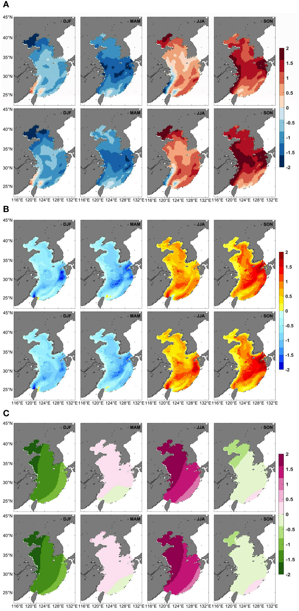
Figure 2 The first CSEOF mode of the combined decomposition represents the annual variability of the three datasets. The seasonally averaged LVs shown in the figure cover a 2-year nested period for satellite altimetry (A), SSLA (B), and DAC (C). Unit: cm. CSEOF, cyclostationary empirical orthogonal function; LV, loading vector; SSLA, Steric Sea Level Anomaly; DAC, Dynamic Atmospheric Correction; DJF, December, January-February; MAM, March-May; JJA, June-August; SON, September-November.

The accompanying PCTS (Figure 3) provides information on the strength of the annual cycle throughout the record. It can be seen that satellite altimetry PCTS has four distinctly low values and three distinctly high values from 1993 to 2020. To calculate the magnitude of the PCTS float of each mode, the mean value of the time series over 28 years was computed. Subsequently, the maximum and minimum values within this series were identified, and their deviations from the mean were calculated. These deviations were then normalized by the mean value to derive the amplitude of the PCTS varies from -15% to 15% from the average.

Figure 3

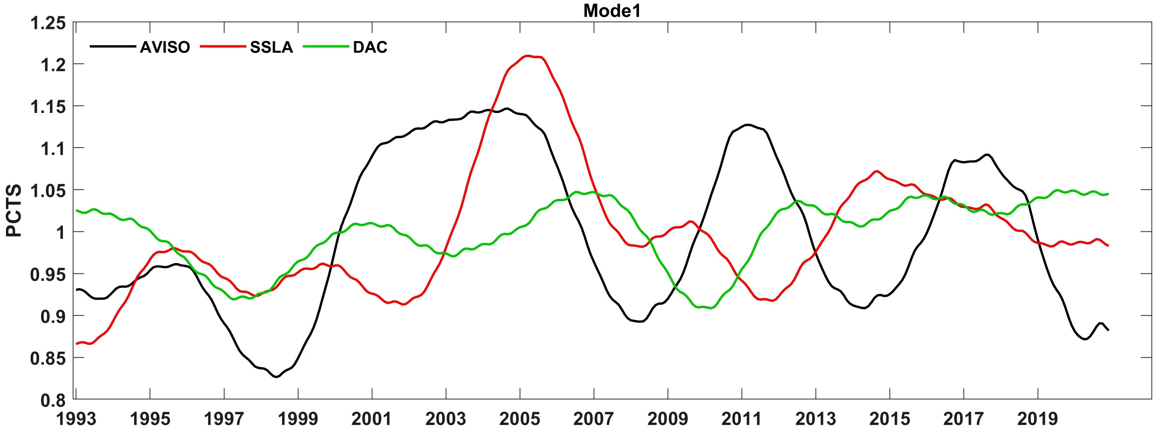
Figure 3 Principal component time series (PCTS) of the first modal correlation, (satellite altimetry (black line), steric sea level anomaly (red line), dynamic atmospheric correction (green line)).

The first mode of the SSLA (depicted in Figure 2B) represents 66.6% of the total variance. Notably, akin to the satellite altimetry sea level anomaly, the variations within the two-year nested cycle are not pronounced. Negative values are predominantly observed during DJF and MAM while contrasting positive values manifest during JJA and SON.

The results of SSLA (Figure 2B) depicted that the BS region shows negative values in DJF and MAM, while positive values in JJA and SON, however, compare to Figure 2A, the variations are not significant. These results suggest that steric sea level not be the primary determinant driving the sea level variations in these areas, aligning with the conclusion drawn by Zhang et al. (2014) and Chang et al. (2017) that the influence of steric effects on the margins of the BS is not markedly significant. We calculated the contribution of steric sea level for the BS region separately, which is 24.3%. To quantitatively analyze the contribution of steric effects, we have reorganized the LVs as presented in Figures 2A, B and the PCTS as depicted in Figure 3, employing Formula (4). The difference between the satellite altimetry sea level and steric sea level were given in Figure 4. It can be seen that the difference between the satellite altimetry sea level and steric sea level is most significant in the BS region (Figure 4), which further indicates that steric is not a primary influence on the sea level variation in the BS. Previous studies have indicated that the influence of winds has a considerable contribution to coastal sea level variations (Dangendorf et al., 2012, 2013). In the BS, in winter northerly winds prevail, resulting in seawater being blown into the ocean and sea level falling in winter. In summer, southeasterly winds prevail, leading to the accumulation of seawater along the coastline (Mao and Sha, 2002) and a significant rise in sea level.

Figure 4

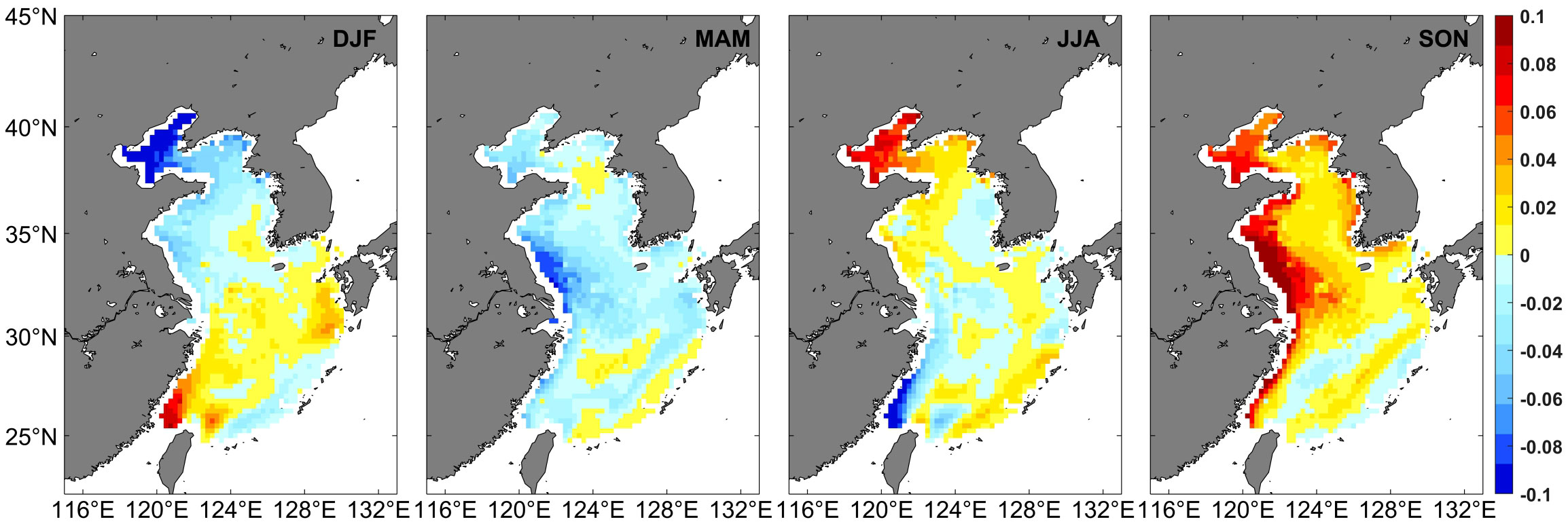
Figure 4 The difference between satellite altimetry sea level and steric sea level after data reorganization. Unit: cm.

The YS region shows negative values in DJF and MAM, while positive values in JJA and SON, and central YS reach the large amplitude SON (Figure 2B). The mean value of the steric contribution of the YS region was 45.7%. While the southern side of the Shandong Peninsula and the Jiangsu coast exhibited the maximum and minimum discrepancies between satellite altimetry sea level and steric sea level in SON and MAM (Figure 4), indicates that steric is not a dominant contribution to sea level variability in shallow nearshore waters. Prior research has underscored the significance of the monsoon, local atmospheric forcing, and wind-driven Ekman transport in influencing the seasonal sea level variability in the Yellow Sea (Marcos et al., 2012; Cheng et al., 2015; Liu et al., 2023). During summer, the YS experiences the influence of the southwesterly monsoon, fostering a northeastward littoral circulation (Liu and Gan, 2014). Conversely, winter brings northerly winds creating a southward pressure gradient, leading to the displacement of the central YS water mass from the shallow Jiangsu coastal waters towards the Kuroshio mainstem, resulting in decreased sea levels (Yuan and Hsueh, 2010). Figure 2C illustrates that the BS/YS region is more susceptible to wind effects during DJF and JJA. The monsoon-induced anomalous flow triggers inward (outward) Ekman transport, thereby causing sea level rises (lowering) (Liu et al., 2023). Furthermore, the northward transportation of the Yangtze River runoff via the YS Cold Water Mass to the Tsushima Strait in Summer contributes to the observed seasonal variations (Liu H. et al., 2021).

The ECS’s eastern region and the Taiwan Strait region exhibit minimal amplitude during DJF. The northern ECS reaches maximum amplitude during SON, while the Taiwan Strait region achieves the maximum amplitude during JJA (Figure 2B). In contrast to the BS and YS, the ECS’s steric sea level change is notably significant, particularly in the Kuroshio basin and the Taiwan Strait region. Independently calculated, the mean value of the steric sea level percentage in the ECS region is 67%. Overall, the disparity between AVISO and SSLA is small, although the Taiwan Strait presents an exception (Figure 4). These findings align with previous conclusions, emphasizing steric sea level as the primary influencing factor of ECS sea level variation. The central and eastern parts of the ECS are influenced by the high-temperature and high-salinity outer seawater introduced by the Kuroshio (Zhang et al., 2014; Chang et al., 2017; Qi et al., 2018; Qu et al., 2023). The Taiwan Strait, due to its shallow depth, is affected by both circulation and local wind (Qi et al., 2017; Liu Z. et al., 2021). In summer, the northward Taiwan warm current intensifies (Yang et al., 2018; Wang et al., 2019), resulting in sea level rises along the coasts of Fujian and Zhejiang. Conversely, in winter, the Fujian-Zhejiang coastal current transports freshwater from the Yangtze River southward, contributing to a reduction in sea level.

The fluctuation of PCTS of steric sea level, when compared with satellite altimetry sea level, exhibits inconsistency between peak and low values across different years (Figure 3). The SSLA PCTS demonstrated a cyclical variation with a 4-6-year periodicity, and it peaked in 2005/2006. The fluctuation trend of SSLA PCTS may be related to the variation of Kuroshio flow. Previous studies have indicated that the Kuroshio flow exhibits an oscillatory cycle varying from 3-5 years (Yu et al., 2008; Qi et al., 2014) and the Kuroshio summer current reached its maximum positive level in 2005 (Qi et al., 2014).

The first modal state of the DAC represents 95.5% of the total variance. The LVs of the DAC (depicted in Figure 2C) illustrate sea level changes that exhibit a more consistent pattern within the two-year nested cycle. Analysis of the figure reveals that the contribution of DAC on the BYECS sea level manifests as a positive anomaly with a substantial amplitude in JJA, a negative anomaly with significant amplitude in DJF, and positive and negative anomalies with smaller amplitudes in MAM and SON, respectively. Seasonal effects decreased from northwest to southeast in all four seasons. The PCTS amplitude of the DAC is not significant compared to the SSLA (Figure 3), and there are periodic oscillations with a period of about 4-6a. With two low values in 1998 and 2010, as 1997/1998 and 2009/2010 belong to the Central Pacific (CP) ENSO, and the Northern Hemisphere winds have a high correlation in response to the CP ENSO events (Capotondi and Ricciardulli, 2021), it is thought that these two low values are in response to CP ENSO events. DAC was applied by AVISO processing algorithms to correct satellite altimetry data. However, here, we found that the variable sea levels forced by high-frequency (less than 20 days) atmospheric wind and pressure, and by low-frequency pressure (more than 20 days) from the static inverted barometer (IB) effect in the annual cycle was also quite large compared with the results from satellite altimeter.

3.2 Trend mode

Sea level change is a non-stationary and non-linear process (Jin et al., 2021), characterized by significant inter-decadal variability influenced by natural physical phenomena. Since the 20th century, the rate of GMSL rise has been on an accelerating trend (Llovel et al., 2019). This acceleration varies across different geographic locations and record periods, leading to disparate acceleration values (Woodworth et al., 2009; Kemp et al., 2011). Additionally, diverse regimes can result in varying response times under the impacts of climate change and acceleration (Camuffo, 2022). Consequently, a trend mode analysis was employed to investigate the trend changes in the BYECS over 28 years, offering insights into the complex non-linear variability of the system.

Figure 5A illustrates the second mode of CSEOF decomposition applied to satellite altimetry data. The analysis reveals that the LV maps exhibit minimal variability throughout the nested period. Furthermore, the derived PCTS, as displayed in Figure 6, demonstrates limited fluctuations around the linear trend. Notably, the trend map excludes the impact of both biennial and low-frequency modes. For discussion within this manuscript, we designate this mode as the “trend mode”.

Figure 5

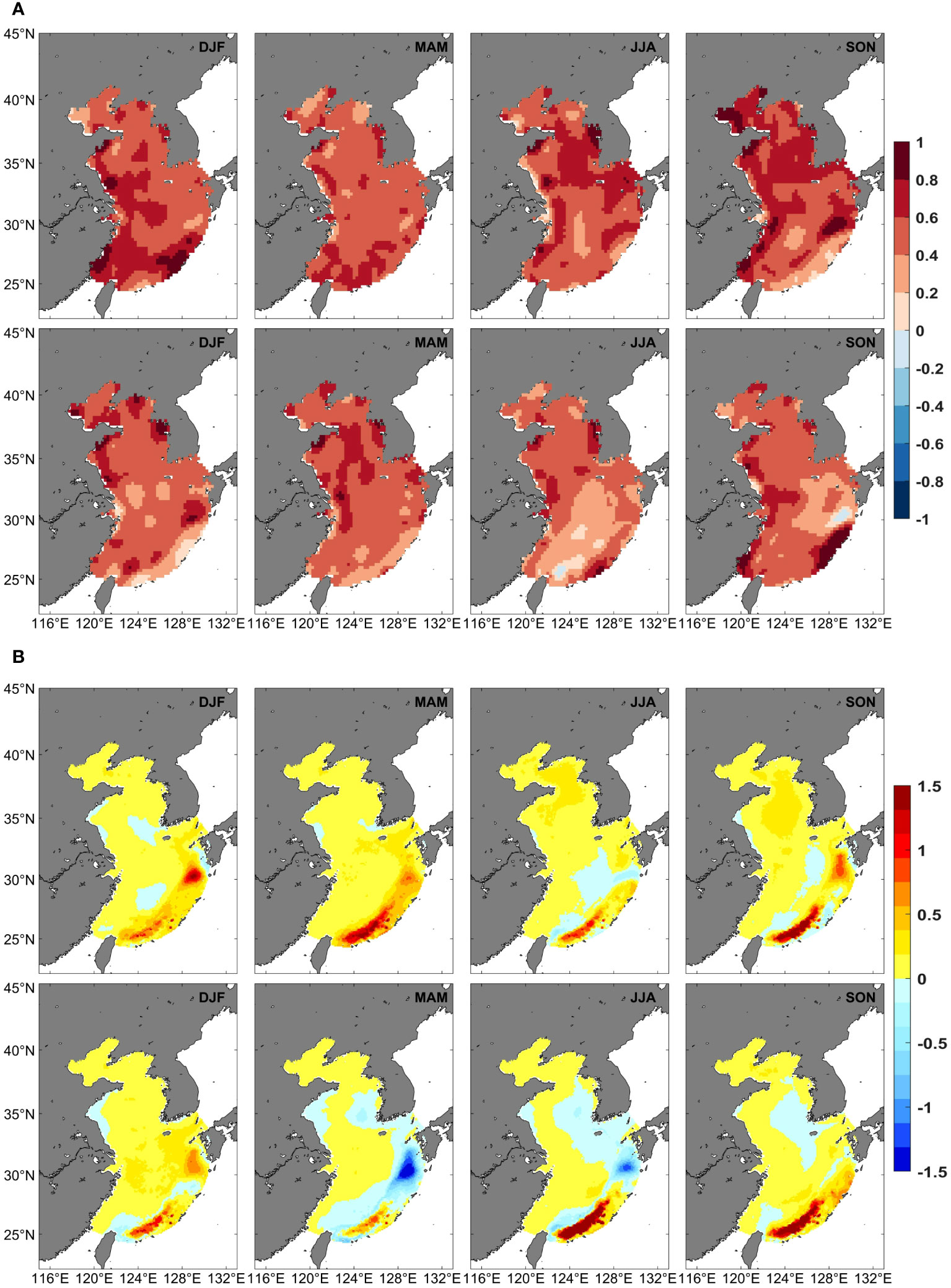
Figure 5 The second CSEOF mode of the combined decomposition represent the trend changes in the two datasets. The seasonally averaged LVs shown cover a 2-year nested period of satellite altimetry (A), SSLA (B). Unit: cm. CSEOF, cyclostationary empirical orthogonal function; LV, load vector; SSLA, Steric Sea Level Anomaly; DJF, December, January-February; MAM, March-May; JJA, June-August; SON, September-November.

Figure 6

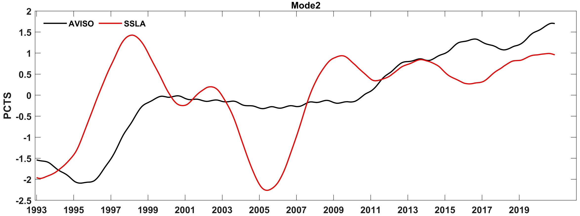
Figure 6 Principal component time series (PCTS) of the second modal correlation (satellite altimetry (black line), steric sea level anomaly (red line)).

In Figure 5A, positive trends in the vast majority of regions in all four seasons, with JJA and SON reaching negative trends in small portions of ECS. Specifically, SON exhibits the maximum amplitude in both the north and south of the BS, while in MAM, the maximum amplitude is reached on the south side of the Shandong Peninsula and the Jiangsu coast. Additionally, the ECS experiences more pronounced variations than BYS during the two-year nested cycle. Notably, the southern part of the ECS demonstrates maximum amplitude during the first year of the nested cycle in DJF, whereas the second year shows values near 0. Furthermore, the southern part of the ECS reaches maximum amplitude in SON and minimum amplitude in the second year of JJA.

The associated PCTS (Figure 6) presents data indicating that satellite altimetry exhibits a distinct positive trend throughout the record since 1996. On the other hand, the SSLA displays multiple fluctuations, while also showcasing a positive trend with a notable slope post-1993 and in 2005/2006.

Similar to the results of the second mode of CSEOF decomposition applied to satellite altimetry data, the second mode of SSLA was also designated as trend mode. Figure 5B illustrates the SSLA, which predominantly exhibits positive anomalies across the four seasons within the nested cycle. Specifically, the northeastern Taiwan Island reaches the maximum amplitude in JJA and SON, while the northeastern ECS reaches the minimum amplitude in MAM.

Figure 7 illustrates the rise rates of satellite altimetry sea level and steric sea level spanning from 1993 to 2020, as well as the disparity between the two. In Figure 7A, the observed sea level trends manifest as positive values, with an average rate of approximately 4 mm/year in the BYS and around 3 mm/year in the central ECS. The disparity in rise rates across the entire BYECS is not substantial, with the maximum value occurring in the south of the Shandong Peninsula. Additionally, the west side of the Korean Peninsula exhibits a maximum rise rate of about 6 mm/year, while near-shelf shallow-water areas such as the Jiangsu, Fujian, and Zhejiang coastlines, as well as the Taiwan Straits, demonstrate a rise rate of approximately 4.5 mm/year.

Figure 7

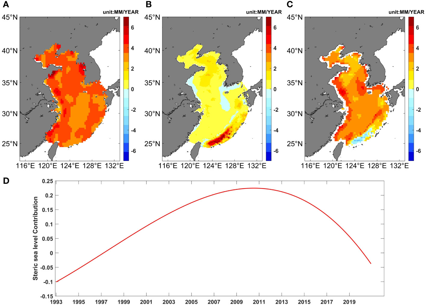
Figure 7 Trends over the period 1993-2020 (satellite altimetry sea level (A), steric sea level (B), difference between the two (C), steric sea level contribution ratio (D)).

In Figure 7B, the rise rates of steric sea level from 1993 to 2020 are depicted. The overall rise rate of steric sea level falls within the range of 0-2 mm/year, with minimal variation observed. Negative values of approximately -1 mm/year are evident in the western YS and the northern part of the ECS, while the Kuroshio Basin exhibits a substantial maximum of 5 mm/year. Notably, a considerable positive acceleration is observed in the Kuroshio region, consistent with the findings of Park et al. (2015) indicating a more pronounced rate of increase in the shallow regions of the YS compared to the deeper regions.

Figure 7C illustrates the disparity between the rates of satellite altimetry sea level and steric sea level. It is evident that in most of the BYECS, except the Kuroshio basin, the satellite altimetry sea level trends surpass the steric sea level trends. This suggests that atmospheric factors, such as wind stress and obliquely-pressurized circulation, may also contribute to the variability of sea level (Marcos et al., 2012).

In Figure 7D, the lines following the LVs and PCTS recombination and the adjusted steric component are fitted to the curves, peaking around 2010, with a proportion ranging from 20% to 25%, with an average value of 11.17%, in line with the findings of Qu et al. (2019). Previous studies also found that increasing ocean mass accounts for a greater proportion of the drivers of sea level change in the BYECS, and it dominates the contribution to the change in sea level trend (Chang et al., 2017; Qu et al., 2023).

3.3 Biennial oscillation mode

The third mode of CSEOF is depicted in Figure 8A. This mode exemplifies a biennial oscillation within the ENSO, specifically characterized by an annual shift between its phases. As described in Hamlington et al. (2016), this type of year-to-year transition was particularly pronounced when a strong El Niño event was succeeded by a robust La Niña episode, as evidenced in the 1997/1998 ENSO cycle.

Figure 8

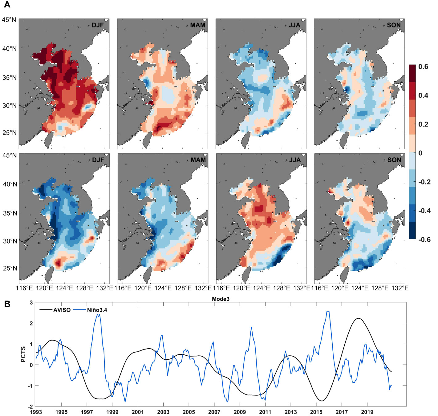
Figure 8 Third CSEOF model of the combined decomposition of satellite altimetry sea level (A). Unit: cm. Principal component time series (PCTS) of the third modal correlation (B). (satellite altimetry (black line), monthly values of the Niño 3.4 index (blue line), CSEOF, cyclostationary empirical orthogonal function; DJF, December, January-February; MAM, March-May; JJA, June-August; SON, September-November).

Upon analyzing Figure 8A, it becomes evident that the LVs within the study area exhibit significant variation during the 2-year nested cycle. Notably, the DJF period demonstrates the most noteworthy variation during this mode, with positive anomalies predominating in the first year, and amplitude maxima occurring in the BS and offshore areas of the YS. Conversely, negative anomalies dominate the second year of the mode, with amplitude minima observed in the southern BS and the Yangtze River estuary, similarly, MAM and JJA also exhibit an overall opposite pattern of LV during the 2 years. The impacts of ENSO exhibit distinctive regional characteristics in the BYECS, with the most pronounced effects observed in the East China Sea, particularly at the continental shelf’s edge. Previous studies have demonstrated that the influence of ENSO on sea levels in the BYECS is more prominent in the southern area than in the northern area (Liu et al., 2010; Zuo et al., 2012). During El Niño events, the northwest wind intensifies, leading to southeastward seawater transport, causing a reduction in sea levels in the southern ECS (Zuo et al., 2012; Wang et al., 2018). Additionally, sea level variation in the southern ECS is notably impacted by the strengthening of the Kuroshio. When the Kuroshio strengthens, the sea level in the ECS typically diminishes, while it rises during periods of Kuroshio weakening (Hwang and Kao, 2002; Kashino et al., 2009; Wang et al., 2014; Zhang et al., 2017).

The results of the monthly value of Niño 3.4 index reflect that the PCTS provides an indication of the significant ENSO events (Figure 8B). During El Niño years, amplitudes diminish, leading to lower sea level heights. Conversely, in the subsequent La Niña years, amplitudes increase, causing sea level heights to gradually rise above normal levels. The PCTS delineates three major valleys occurring in 1997/1998, 2009/2010, and 2015/2016, aligning with the timing of strong El Niño events. Furthermore, the PCTS exhibited a considerable decline from late 1997 to early 1998 and from late 2015 to early 2016, corresponding to these strong El Niño occurrences, followed by a rapid resurgence from late 1998 to 1999 and early 2017, aligning with the ensuing La Niña phenomenon.

4 Summary

The social, cultural, and natural ecosystems of the coastal regions bordering the Bohai, Yellow Sea, and East China Sea (BYECS) are significantly impacted by irregular sea level fluctuations and the recurrent occurrence of catastrophic events. It is imperative to comprehend the variability of sea level to accurately estimate and predict regional sea level rise in the coming decades. Quantifying and assessing the principal mechanisms of sea level change has long posed a significant challenge in marine research. In this study, we endeavor to differentiate the primary sea level variability modes from satellite altimetry data employing the CSEOF analysis method. Additionally, we utilize steric sea level data and DAC data as auxiliary sources for simultaneous processing. The ensuing analysis yields the following primary conclusions.

The sea level in the BYECS exhibits pronounced seasonal variations, and the amplitude of the annual cycle displays a non-stationary signal, fluctuating between -15% and 15% from the average. Winter and spring denote periods of lower sea level, while summer and fall exhibit higher sea levels. On a spatial scale, the nearshore shallow waters of the BS, Jiangsu, Zhejiang, and Fujian are particularly susceptible to seawater volume changes. In contrast, the southern YS and the eastern ECS, especially the Kuroshio flow area, are significantly impacted by steric effects. The seasonal characteristics of the Dynamic Atmosphere and Ocean Coupling’s (DAC) influence on sea level in the BYECS are notable, with a more pronounced influence observed during winter and summer.

The satellite altimetry sea level exhibits an average trend within the range of 3-4 mm/year, with the most substantial trend observed in the south of the Shandong Peninsula and the eastern YS, reaching 5-6 mm/year. Conversely, the steric sea level trend is generally smaller, falling within the range of 0-2 mm/year. Throughout the entire period, the contribution of steric sea level to the mean sea level trend was consistently less than 25%.

BYECS sea level fluctuations are strongly sensitive to strong El Niño years, and the impacts exhibit distinct regional variations. This influence is manifested through the intricate interplay of atmospheric circulation on local wind stresses and ocean circulation on sea level fluctuations in the BYECS.

In this paper, we make an effort to distinguish the primary sea level variability modes of the BYECS from satellite altimetry data using the CSEOF analysis method. This approach facilitated a more nuanced comprehension of sea level variability in the BYECS, particularly highlighting the annual cycle of sea level amplitude and the influences of the Biennial Oscillation. Nonetheless, further research is imperative to disaggregate the contributions of diverse factors to sea level variability.

Data availability statement

The original contributions presented in the study are included in the article/Supplementary Material. Further inquiries can be directed to the corresponding authors.

Author contributions

YL: Writing – original draft, Validation, Software, Data curation. JF: Writing – review & editing, Supervision, Resources, Methodology. XY: Writing – review & editing, Validation, Software. SZ: Writing – review & editing, Validation, Software. GC: Writing – review & editing, Validation, Software. LZ: Writing – review & editing, Supervision, Resources. HF: Writing – review & editing, Validation, Resources.

Funding

The author(s) declare financial support was received for the research, authorship, and/or publication of this article. This work is supported by National Natural Science Foundation of China (grants 42176198) and this work is supported by National Key Research and Development Program of China (grant number 2022YFC3105000).

Acknowledgments

The authors would like to thank the organizations that provided data for this work, including the National Marine Data Center of China, AVISO (Archiving, Validation and Interpretation of Satellite Oceanographic) and the National Oceanic and Atmospheric Administration (NOAA). The steric data is through the website of the National Marine Data Center of China (https://mds.nmdis.org.cn/pages/dataView.html?type=2&id=a5da2a0528904471b3a326c3cc85997d); The Niño3.4 monthly value data is through the NOAA Physical Sciences Laboratory website (psl.noaa.gov/gcos_wgsp/Timeseries/Nino34/).

Conflict of interest

The authors declare that the research was conducted in the absence of any commercial or financial relationships that could be construed as a potential conflict of interest.

Publisher’s note

All claims expressed in this article are solely those of the authors and do not necessarily represent those of their affiliated organizations, or those of the publisher, the editors and the reviewers. Any product that may be evaluated in this article, or claim that may be made by its manufacturer, is not guaranteed or endorsed by the publisher.

Supplementary material

The Supplementary Material for this article can be found online at: https://www.frontiersin.org/articles/10.3389/fmars.2024.1381187/full#supplementary-material

References

Araújo I. B., Pugh D. T. (2008). Sea levels at newlyn 1915–2005: analysis of trends for future flooding risks. J. Coast. Res. 24, 203–212. doi: 10.2112/06-0785.1

CrossRef Full Text | Google Scholar

Bai Z. P., Han J., Guo X. P., Zhu K. L. (2020). Spatial and temporal distribution characteristics of mesoscale eddies in the South China Sea based on the CORA2 reanalysis data. Mar. Forecast. 37, 73–83. doi: 10.11737/j.issn.1003-0239.2020.02.009

CrossRef Full Text | Google Scholar

Bouttes N., Gregory J. M., Kuhlbrodt T., Smith R. S. (2014). The drivers of projected North Atlantic sea level change. Clim. Dyn. 43, 1531–1544. doi: 10.1007/s00382-013-1973-8

CrossRef Full Text | Google Scholar

Camuffo D. (2022). A discussion on sea level rise, rate ad acceleration. Venice as a case study. Environ. Earth Sci. 81, 349. doi: 10.1007/s12665-022-10482-x

CrossRef Full Text | Google Scholar

Capotondi A., Ricciardulli L. (2021). The influence of Pacific winds on ENSO diversity. Sci. Rep. 11, 18672. doi: 10.1038/s41598-021-97963-4

PubMed Abstract | CrossRef Full Text | Google Scholar

Carrère L., Lyard F. (2003). Modeling the barotropic response of the global ocean to atmospheric wind and pressure forcing-comparisons with observations. Geophys. Res. Lett. 30, 1275. doi: 10.1029/2002GL016473

CrossRef Full Text | Google Scholar

Carson M., Köhl A., Stammer D., Meyssignac B., Church J., Schröter J., et al. (2017). Regional sea level variability and trends 1960–2007: A comparison of sea level reconstructions and ocean syntheses. J. Geophys. Res. Ocean. 122, 9068–9091. doi: 10.1002/2017JC012992

CrossRef Full Text | Google Scholar

Carton J. A., Giese B. S., Grodsky S. A. (2005). Sea level rise and the warming of the oceans in the Simple Ocean Data Assimilation (SODA) ocean reanalysis. J. Geophys. Res. Ocean. 110, C09006. doi: 10.1029/2004JC002817

CrossRef Full Text | Google Scholar

Cazenave A., Cozannet G. L. (2014). Sea level rise and its coastal impacts. Earths Future 2, 15–34. doi: 10.1002/2013EF000188

CrossRef Full Text | Google Scholar

Cazenave A., Llovel W. (2010). Contemporary sea level rise. Annu. Rev. Mar. Sci. 2, 145–173. doi: 10.1146/annurev-marine-120308-081105

CrossRef Full Text | Google Scholar

Chambers D. P. (2006). Observing seasonal steric sea level variations with GRACE and satellite altimetry. J. Geophys. Res. Ocean. 111, C03010. doi: 10.1029/2005JC002914

CrossRef Full Text | Google Scholar

Chang L., Qain A., Yi S., Xu C. Y., Sun W. K. (2017). Sea level change in China adjacent seas studied using satellite altimeter, satellite, gravity, and thermohaline data. J. Univ. China Sci. 34, 371–379. doi: 10.7523/j.issn.2095-6134.2017.03.011

CrossRef Full Text | Google Scholar

Chao G., Wu X., Zhang L., Fu H., Liu K., Han G. (2021). China ocean reanalysis products and validation for 2009–18. AOSL 14, 100023. doi: 10.1016/j.aosl.2020.100023

CrossRef Full Text | Google Scholar

Chen X., Zhang X., Church J. A., Watson C. S., King M. A., Monselesan D., et al. (2017). The increasing rate of global mean sea-level rise during 1993–2014. Nat. Clim. Change 7, 492–495. doi: 10.1038/nclimate3325

CrossRef Full Text | Google Scholar

Cheng Y., Hamlington B. D., Plag H.-P., Xu Q. (2016). Influence of ENSO on the variation of annual sea level cycle in the South China Sea. Ocean Eng. 126, 343–352. doi: 10.1016/j.oceaneng.2016.09.019

CrossRef Full Text | Google Scholar

Cheng X., Li L., Du Y., Wang J., Huang R. X. (2013). Mass-induced sea level change in the northwestern North Pacific and its contribution to total sea level change. Geophys. Res. Lett. 40, 3975–3980. doi: 10.1002/grl.50748

CrossRef Full Text | Google Scholar

Cheng Y., Plag H. P., Hamlington B. D., Xu Q., He Y. (2015). Regional sea level variability in the Bohai Sea, Yellow Sea, and East China Sea. Cont. Shelf. Res. 111, 95–107. doi: 10.1016/j.csr.2015.11.005

CrossRef Full Text | Google Scholar

Cheon S. H., Hamlington B. D., Reager J. T., Chandanpurkar H. A. (2021). Identifying ENSO-related interannual and decadal variability on terrestrial water storage. Sci. Rep. 11, 13595. doi: 10.1038/s41598-021-92729-4

PubMed Abstract | CrossRef Full Text | Google Scholar

Church J. A., Clark P. U., Cazenave A., Gregory J. M., Jevrejeva S., Levermann A., et al. (2013). “Sea level change, in: Climate Change 2013,” in The physical science basis, contribution of working group I to the fifth assessment report of the intergovernmental panel on climate change. Ed. Stocker T. F., et al. (Cambridge University Publishing, Cambridge, United Kingdom and New York, NY, USA).

Google Scholar

Cui M., Zorita E. (1998). Analysis of the sea-level variability along the Chinese coast and estimation of the impact of a CO2-perturbed atmospheric circulation. Tellus A. 50, 333–347. doi: 10.3402/tellusa.v50i3.14530

CrossRef Full Text | Google Scholar

Cummins P. F., Lagerloef G. S. E. (2004). Wind-driven interannual variability over the northeast Pacific Ocean. Deep Sea Res. Part I. 51, 2105–2121. doi: 10.1016/j.dsr.2004.08.004

CrossRef Full Text | Google Scholar

Dangendorf S., Mudersbach C., Wahl T., Jensen J. (2013). Characteristics of intra-, inter-annual and decadal sea-level variability and the role of meteorological forcing: the long record of Cuxhaven. Ocean Dyn. 63, 209–224. doi: 10.1007/s10236-013-0598-0

CrossRef Full Text | Google Scholar

Dangendorf S., Wahl T., Hein H., Jensen J., Mai S., Mudersbach C. (2012). Mean sea level variability and influence of the North Atlantic oscillation on long-term trends in the German Bight. Water 4, 170–195. doi: 10.3390/w4010170

CrossRef Full Text | Google Scholar

Feng M., Böning C., Biastoch A., Behrens E., Weller E., Masumoto Y. (2011). The reversal of the multi-decadal trends of the equatorial Pacific easterly winds, and the Indonesian Throughflow and Leeuwin Current transports. Geophys. Res. Lett. 38, L11604. doi: 10.1029/2011GL047291

CrossRef Full Text | Google Scholar

Forget G., Ponte R. M. (2015). The partition of regional sea level variability. Prog. Oceanogr. 137, 173–195. doi: 10.1016/j.pocean.2015.06.002

CrossRef Full Text | Google Scholar

Fu H., Dan B., Gao Z., Wu X., Chao G., Zhang L. (2023). Global ocean reanalysis CORA2 and its inter comparison with a set of other reanalysis products. Front. Mar. Sci. 10. doi: 10.3389/fmars.2023.1084186

CrossRef Full Text | Google Scholar

Gardiner S., Hanson S. E., Nicholls R. J., Zhang Z., Jude S., Jones A. P., et al. (2007). The habitats directive, coastal habitats and climate change - case studies from the south coast of the U.K. Proceedings of the two-day international conference organized by the institution of civil engineers and held in Cardiff on 31th October-1st November 2007 (London, UK: Thomas Telford Publishing).

Google Scholar

Gill A. E., Niller P. P. (1973). The theory of the seasonal variability in the ocean. Deep-Sea Res. Ocean. 20, 141–177. doi: 10.1016/0011-7471(73)90049-1

CrossRef Full Text | Google Scholar

Hamlington B. D., Burgos A. G., Thompson P. R., Landerer F. W., Piecuch C. G., Adhikari S., et al. (2018). Observation driven estimation of the spatial variability of 20th century sea level rise. J. Geophys. Res. 123, 2129–2140. doi: 10.1002/2017JC013486

CrossRef Full Text | Google Scholar

Hamlington B. D., Cheon S. H., Piecuch C. G., Karnauskas K. B., Thompson P. R., Kim K. Y., et al. (2019a). The dominant global modes of recent internal sea level variability. J. Geophys. Res. Ocean. 124, 2750–2768. doi: 10.1029/2018JC014635

CrossRef Full Text | Google Scholar

Hamlington B. D., Cheon S. H., Thompson P. R., Merrifield M. A., Nerem R. S., Leben R. R., et al. (2016). An ongoing shift in Pacific Ocean sea level. J. Geophys. Res. Ocean. 121, 5084–5097. doi: 10.1002/2016JC011815

CrossRef Full Text | Google Scholar

Hamlington B. D., Fasullo J. T., Nerem R. S., Kim K. Y., Landerer F. W. (2019b). Uncovering the pattern of forced sea level rise in the satellite altimeter record. Geophys. Res. Lett. 46, 4844–4853. doi: 10.1029/2018GL081386

CrossRef Full Text | Google Scholar

Hamlington B. D., Leben R. R., Kim K. Y., Nerem R. S., Atkinson L. P., Thompson P. R. (2015). The effect of the El Niño-Southern Oscillation on U.S. regional and coastal sea level. J. Geophys. Res. Ocean. 120, 3970–3986. doi: 10.1002/2014JC010602

CrossRef Full Text | Google Scholar

Hamlington B. D., Leben R. R., Nerem R. S., Han W., Kim K. Y. (2011). Reconstructing sea level using cyclostationary empirical orthogonal functions. J. Geophys. Res. Ocean. 116, C12015. doi: 10.1029/2011JC007529

CrossRef Full Text | Google Scholar

Hamlington B. D., Leben R. R., Strassburg M. W., Kim K. Y. (2014). Cyclostationary empirical orthogonal function sea-level reconstruction. Geosci. Data J. 1, 13–19. doi: 10.1002/gdj3.6

CrossRef Full Text | Google Scholar

Hamlington B. D., Leben R. R., Wright L. A., Kim K. Y. (2012). Regional sea level reconstruction in the Pacific Ocean. Mar. Geod. 35, 117–198. doi: 10.1080/01490419.2012.718210

CrossRef Full Text | Google Scholar

Han G., Huang W. (2008). Pacific decadal oscillation and sea level variability in the Bohai, Yellow, and East China Seas. J. Phys. Oceanogr. 38, 2772–2783. doi: 10.1175/2008JPO3885.1

CrossRef Full Text | Google Scholar

Han G., Li W., Zhang X., Li D., He Z., Wang X., et al. (2011). A regional ocean reanalysis system for coastal waters of China and adjacent seas. Adv. Atmos. Sci. 28, 682–690. doi: 10.1007/s00376-010-9184-2

CrossRef Full Text | Google Scholar

Hay J. E., Mimura N. (2005). Sea level rise: implications for water resources management. Mitig. Adapt. Strateg. Glob. Change 10, 717–737. doi: 10.1007/s11027-005-7305-5

CrossRef Full Text | Google Scholar

Hochet A., Llovel W., Sévellec F., Huck T. (2023). Sources and sinks of interannual steric sea level variability. J. Geophys. Res. Ocean. 128, e2022JC019335. doi: 10.1029/2022JC019335

CrossRef Full Text | Google Scholar

Hwang C., Kao R. (2002). TOPEX/POSEIDON-derived space-time variations of the Kuroshio Current: applications of a gravimetric geoid and wavelet analysis. Geophys. J. Int. 151, 835–847. doi: 10.1046/j.1365-246X.2002.01811.x

CrossRef Full Text | Google Scholar

Jin T., Xiao M., Jiang W., Shum C. K., Ding H., Kuo C. Y., et al. (2021). An adaptive method for nonlinear sea level trend estimation by combining EMD and SSA. Earth Space Sci. 8, e2020EA001300. doi: 10.1029/2020EA001300

CrossRef Full Text | Google Scholar

Kashino Y., España N., Syamsudin F., Richards K. J., Jensen T., Dutrieux P., et al. (2009). Observations of the North Equatorial Current, Mindanao Current, and Kuroshio current system during the 2006/07 El Niño and 2007/08 La Niña. J. Oceanogr. 65, 325–333. doi: 10.1007/s10872-009-0030-z

CrossRef Full Text | Google Scholar

Kemp A. C., Horton B. P., Donnelly J. P., Mann M. E., Vermeer M., Rahmstorf S. (2011). Climate related sea-level variations over the past two millennia. PNAS 108, 11017–11022. doi: 10.1073/pnas.1015619108

PubMed Abstract | CrossRef Full Text | Google Scholar

Kim K. Y., Hamlington B., Na H. (2015). Theoretical foundation of cyclostationary EOF analysis for geophysical and climatic variables: concepts and examples. Earth Sci. Rev. 150, 201–218. doi: 10.1016/j.earscirev.2015.06.003

CrossRef Full Text | Google Scholar

Kim K. Y., North G. R. (1997). EOFs of harmonizable cyclostationary processes. J. Atmos. Sci. 54, 2416–2427. doi: 10.1175/1520-0469(1997)054<2416:EOHCP>2.0.CO;2

CrossRef Full Text | Google Scholar

Kim K. Y., North G. R., Huang J. (1996). EOFs of one-dimensional cyclostationary time series: computations, examples, and stochastic modeling. J. Atmos. Sci. 53, 1007–1017. doi: 10.1175/1520-0469(1996)053<1007:eoodct>2.0.co;2

CrossRef Full Text | Google Scholar

Kim K. Y., Wu Q. (1999). A comparison study of EOF techniques: analysis of nonstationary data with periodic statistics. J. Clim. 12, 185–199. doi: 10.1175/1520-0442(1999)012<0185:ACSOET>2.0.CO;2

CrossRef Full Text | Google Scholar

Kumar P., Hamlington B., Cheon S. H., Han W., Thompson P. (2020). 20th century multivariate Indian Ocean regional sea level reconstruction. J. Geophys. Res. Ocean. 125, e2020JC016270. doi: 10.1029/2020JC016270

CrossRef Full Text | Google Scholar

Lan W. H., Kuo C. Y., Lin L. C., Kao H. C. (2021). Annual sea level amplitude analysis over the north pacific ocean coast by ensemble empirical mode decomposition method. Remote Sens. 13, 730. doi: 10.3390/rs13040730

CrossRef Full Text | Google Scholar

Leuliette E. W. (2015). The balancing of the sea-level budget. Curr. Clim. Change Rep. 1, 185–191. doi: 10.1007/s40641-015-0012-8

CrossRef Full Text | Google Scholar

Leuliette E. W., Willis J. K. (2011). Balancing the sea level budget. Oceanography 24, 122–129. doi: 10.5670/oceanog.2011.32

CrossRef Full Text | Google Scholar

Liu H., Cheng X., Qin J., Zhou G., Jiang L. (2023). The dynamic mechanism of sea level variations in the Bohai Sea and Yellow Sea. Clim. Dyn. 61, 2937–2947. doi: 10.1007/s00382-023-06724-8

CrossRef Full Text | Google Scholar

Liu H., Feng X., Tao A., Zhang W. (2021). Intraseasonal variability of sea level in the western North Pacific. J. Geophys. Res. Ocean. 126, e2021JC017237. doi: 10.1029/2021JC017237

CrossRef Full Text | Google Scholar

Liu Z., Gan J. (2014). Modeling study of variable upwelling circulation in the East China Sea: response to a coastal promontory. J. Phys. Oceanogr. 44, 1078–1094. doi: 10.1175/JPO-D-13-0170.1

CrossRef Full Text | Google Scholar

Liu Z., Gan J., Hu J., Wu H., Cai Z., Deng Y. (2021). Progress of studies on circulation dynamics in the East China Sea: the Kuroshio exchanges with the shelf currents. Front. Mar. Sci. 8. doi: 10.3389/fmars.2021.620910

CrossRef Full Text | Google Scholar

Liu X., Liu Y., Guo L., Rong Z., Gu Y., Liu Y. (2010). Interannual changes of sea level in the two regions of East China Sea and different responses to ENSO. Glob. Planet Change. 72, 215–226. doi: 10.1016/j.gloplacha.2010.04.009

CrossRef Full Text | Google Scholar

Llovel W., Purkey S., Meyssignac B., Blazquez A., Kolodziejczyk N., Bamber J. (2019). Global ocean freshening, ocean mass increase and global mean sea level rise over 2005–2015. Sci. Rep. 9, 17717. doi: 10.1038/s41598-019-54239-2

PubMed Abstract | CrossRef Full Text | Google Scholar

Mao Y., Sha W. Y. (2002). Effect of sea surface wind field on the thermocline in sea area around Taiwan Island. Mar. Forecast. 19, 33–43. doi: 10.3969/j.issn.1003-0239.2002.03.004

CrossRef Full Text | Google Scholar

Marcos M., Tsimplis M. N., Calafat F. M. (2012). Inter-annual and decadal sea level variations in the north-western Pacific marginal seas. Prog. Oceanogr. 105, 4–21. doi: 10.1016/j.pocean.2012.04.010

CrossRef Full Text | Google Scholar

Marzeion B., Jarosch A. H., Hofer M. (2012). Past and future sea-level change from the surface mass balance of glaciers. Cryosphere 6, 1295–1322. doi: 10.5194/tc-6-1295-2012

CrossRef Full Text | Google Scholar

Mason S. A., Hamlington P. E., Hamlington B. D., Matt Jolly W., Hoffman C. M. (2017). Effects of climate oscillations on wildland fire potential in the continental United States. Geophys. Res. Lett. 44, 7002–7010. doi: 10.1002/2017GL074111

CrossRef Full Text | Google Scholar

McDougall T. J., Barker P. M. (2011). Getting started with TEOS-10 and the gibbs seawater (GSW) oceanographic toolbox. Scor/Iapso Wg 127, 28.

Google Scholar

Meyssignac B., Piecuch C. G., Merchant C. J., Racault M. F., Palanisamy H., MacIntosh C., et al. (2017). Causes of the regional variability in observed sea level, sea surface temperature and ocean colour over the period 1993–2011. Surv. Geophys. 38, 187–215. doi: 10.1007/s10712-016-9383-1

CrossRef Full Text | Google Scholar

Mohamed B., Skliris N. (2022). Steric and atmospheric contributions to interannual sea level variability in the eastern Mediterranean Sea over 1993–2019. Oceanologia 64, 50–62. doi: 10.1016/j.oceano.2021.09.001

CrossRef Full Text | Google Scholar

Park K. A., Lee E. Y., Chang E., Hong S. (2015). Spatial and temporal variability of sea surface temperature and warming trends in the Yellow Sea. J. Mar. Syst. 143, 24–38. doi: 10.1016/j.jmarsys.2014.10.013

CrossRef Full Text | Google Scholar

Pawlowicz R., McDougall T., Feistel R., Tailleux R. (2012). An historical perspective on the development of the thermodynamic equation of seawater - 2010. Ocean Sci. 8, 161–174. doi: 10.5194/os-8-161-2012

CrossRef Full Text | Google Scholar

Pei Y. (2021). Cyclostationary EOF modes of antarctic sea ice and their application in prediction. J. Geophys. Res. Ocean. 126, e2021JC017179. doi: 10.1029/2021JC017179

CrossRef Full Text | Google Scholar

Qi J., Yin B., Xu Z., Li D. (2018). Spatiotemporal variations of the surface Kuroshio east of Taiwan Island derived from satellite altimetry data. J. Oceanol. Limnol. 36, 77–91. doi: 10.1007/s00343-018-6314-7

CrossRef Full Text | Google Scholar

Qi J., Yin B., Yang D. Z., Xu Z. H. (2014). The inter-annusal and inter-decadal variability of the Kuroshio volume transport in the East China Sea. Oceanol. Limnol. Sin. 45, 1141–1147. doi: 10.11693/hyhz20140100025

CrossRef Full Text | Google Scholar

Qi J., Yin B., Zhang Q., Yang D., Xu Z. (2017). Seasonal variation of the Taiwan Warm Current Water and its underlying mechanism. J. Oceanol. Limnol. 35, 1045–1060. doi: 10.1007/s00343-017-6018-4

CrossRef Full Text | Google Scholar

Qu Y., Jevrejeva S., Wang S. (2023). Unraveling regional patterns of sea level acceleration over the China seas. Remote Sens. 15, 4448. doi: 10.3390/rs15184448

CrossRef Full Text | Google Scholar

Qu Y., Jevrejeva S., Jackson L. P., Moore J. C. (2019). Coastal sea level rise around the china seas. Glob Planet Change. 172, 454–463. doi: 10.1016/j.gloplacha.2018.11.005

CrossRef Full Text | Google Scholar

Ranjan S. P., Kazama S., Sawamoto M. (2006). Effects of climate and land use changes on groundwater resources in coastal aquifers. J. Environ. Manage. 80, 25–35. doi: 10.1016/j.jenvman.2005.08.008

PubMed Abstract | CrossRef Full Text | Google Scholar

Schneider D. P., Deser C., Fasullo J., Trenberth K. E. (2013). Climate data guide spurs discovery and understanding. Eos Trans. 94, 121–122. doi: 10.1002/2013eo130001

CrossRef Full Text | Google Scholar

Shepherd A., Ivins E. R., A G., Barletta V. R., Bentley M. J., Bettadpur S., et al. (2012). A reconciled estimate of ice-sheet mass balance. Science 338, 1183–1189. doi: 10.1126/science.1228102

PubMed Abstract | CrossRef Full Text | Google Scholar

Stammer D., Cazenave A., Ponte R. M., Tamisiea M. E. (2013). Causes for contemporary regional sea level changes. Ann. Rev. Mar. Sci. 5, 21–46. doi: 10.1146/annurev-marine-121211-172406

PubMed Abstract | CrossRef Full Text | Google Scholar

Wang G., Cheng L., Boyer T., Li C. (2017). Halosteric sea level changes during the Argo era. Water 9, 484. doi: 10.3390/w9070484

CrossRef Full Text | Google Scholar

Wang X. H., Cho Y. K., Guo X., Wu C. R., Zhou J. (2015). The status of coastal oceanography in heavily impacted Yellow and East China Sea: past trends, progress, and possible futures. Estuar. Coast. Shelf. Sci. 163, 235–243. doi: 10.1016/j.ecss.2015.05.039

CrossRef Full Text | Google Scholar

Wang G., Kang J., Yan G., Han G., Han Q. (2015). Spatio-temporal variability of sea level in the East China Sea. J. Coast. Res. 73, 40–47. doi: 10.2112/SI73-008.1

CrossRef Full Text | Google Scholar

Wang H., Liu K., Wang A., Feng J., Fan W., Liu Q., et al. (2018). Regional characteristics of the effects of the El Niño-Southern Oscillation on the sea level in the China Sea. Ocean Dyn. 68, 485–495. doi: 10.1007/s10236-018-1144-x

CrossRef Full Text | Google Scholar

Wang L., Wang J., Yang J. G. (2014). The comprehensive analysis of sea level change in the East China Sea. Acta Ocranol. Sin. 36, 28–37. doi: 10.3969/j.issn.0253-4193.2014.01.004

CrossRef Full Text | Google Scholar

Wang J., Yu F., Ren Q., Si G., Wei C. (2019). The observed variations of the north intrusion of the bottom Taiwan Warm Current inshore branch and its response to wind. Reg. Stud. Mar. Sci. 30, 100690. doi: 10.1016/j.rsma.2019.100690

CrossRef Full Text | Google Scholar

Watson C. S., White N. J., Church J. A., King M. A., Burgette R. J., Legresy B. (2015). Unabated global mean sea-level rise over the satellite altimeter era. Nat. Clim. Change 5, 565–568. doi: 10.1038/nclimate2635

CrossRef Full Text | Google Scholar

Woodworth P., Morales Maqueda M. Á., Gehrels W., Roussenov V., Williams R., Hughes C. (2017). Variations in the difference between mean sea level measured either side of cape hatteras and their relation to the North Atlantic Oscillation. Clim. Dyn. 49, 2451–2469. doi: 10.1007/s00382-016-3464-1

CrossRef Full Text | Google Scholar

Woodworth P. L., White N. J., Jevrejeva S., Holgate S. J., Church J. A., Gehrels W. R. (2009). Evidence for the accelerations of sea level on multi-decade and century timescales. Int. J. Climatol. 29, 777–789. doi: 10.1002/joc.1771

CrossRef Full Text | Google Scholar

Wu C., Hsin Y., Chiang T., Lin Y., Tsui I. (2014). Seasonal and interannual changes of the Kuroshio intrusion onto the East China Sea Shelf. J. Geophys. Res. Ocean. 119, 5039–5051. doi: 10.1002/2013JC009748

CrossRef Full Text | Google Scholar

Yanagi T., Akaki T. (1994). Sea level variation in the eastern Asia. J. Oceanogr. 50, 643–651. doi: 10.1007/BF02270497

CrossRef Full Text | Google Scholar

Yang Y., Lyu W., Sun Q. (2018). Temporal and spatial variation of sea level in the East China Sea during 1993-2015. Conf. Ser.: Earth Environ. Sci. 170, 32015. doi: 10.1088/1755-1315/170/3/032015

CrossRef Full Text | Google Scholar

Yeo S. R., Kim K. Y. (2014). Global warming, low-frequency variability, and biennial oscillation: an attempt to understand the physical mechanisms driving major ENSO events. Clim. Dyn. 43, 771–786. doi: 10.1007/s00382-013-1862-1

CrossRef Full Text | Google Scholar

Yu F., Wang Q., Liu Y. L. (2008). The seasonal and interannual variations of the upper Kuroshio circulation in the East China Sea and their relationship with local wind stress. J. Ocean Univ. China 38, 533–538. doi: 10.16441/j.cnki.hdxb.2008.04.003

CrossRef Full Text | Google Scholar

Yuan D., Hsueh Y. (2010). Dynamics of the cross-shelf circulation in the Yellow and East China Seas in winter. Deep Sea Res. Part II Top. Stud. Oceanogr. 57, 1745–1761. doi: 10.1016/j.dsr2.2010.04.002

CrossRef Full Text | Google Scholar

Zhang J., Guo X., Zhao L., Miyazawa Y., Sun Q. (2017). Water exchange across isobaths over the continental shelf of the east china sea. J. Phys. Oceanogr. 47 (5), 1043–1060. doi: 10.1175/JPO-D-16-0231.1

CrossRef Full Text | Google Scholar

Zhang X., Church J. A. (2012). Sea level trends, interannual and decadal variability in the Pacific Ocean. Geophys. Res. Lett. 39, L21701. doi: 10.1029/2012GL053240

CrossRef Full Text | Google Scholar

Zhang S., Du L., Wang H., Jiang H. (2014). Regional sea level variation on interannual timescale in the East China Sea. Int. J. Geosci. 05, 1405–1414. doi: 10.4236/ijg.2014.512114

CrossRef Full Text | Google Scholar

Zuo J. C., He Q. Q., Chen C., Chen M., Xu Q. (2012). Sea level variability in East China Sea and its response to ENSO. Water Sci. Eng. 5, 164–174. doi: 10.3882/j.issn.1674-2370.2012.02.005

CrossRef Full Text | Google Scholar