Integrated drag coefficient formula for estimating the wave attenuation capacity of Rhizophora sp. mangrove forests

1 Introduction

Mangroves are intertidal ecosystems that are present in tropical and subtropical regions. They provide several ecosystem services, such as carbon sequestration, animal habitat and water quality improvement (Ewel et al., 1998; Duarte et al., 2013; Mitsch et al., 2015). These ecosystems also function as natural barriers to wave action (Menéndez et al., 2018; Temmerman et al., 2022) and contribute to shoreline stabilization (McIvor et al., 2012; Gijsman et al., 2021; van Hespen et al., 2023). The coastal protection that this vegetation offers varies according to the life stage of the mangrove, geographic location and the environmental features to which it is exposed (Lugo et al., 1974; Koch et al., 2009; Maza et al., 2021). Consequently, quantifying the coastal protection services provided by mangroves is challenging due to the heterogeneity of ecosystem properties and flow conditions.

To better understand the coastal protection services provided by these ecosystems, several studies have identified key hydrodynamic (e.g., water depth, wave height and period) and ecological (e.g., species, forest width, density, root and trunk diameter, vegetation height) factors that influence the evolution of wave height across forests (Gijsman et al., 2021) by using either laboratory tests (e.g., Maza et al., 2019; Chang et al., 2022; Kelty et al., 2022) or field measurements (e.g., Mazda et al., 2006; Quartel et al., 2007; Horstman et al., 2014; Norris et al., 2017). Furthermore, the ability of mangroves to attenuate waves has been estimated by numerical modeling (Suzuki et al., 2012). The most common numerical models used for simulating wave attenuation by vegetation are based on the definition of the drag force exerted by plants, which depends on the correct selection of a bulk drag coefficient (${\tilde{C}}_D$), and the geometric characteristics of the mangrove forest.

Typically, ${\tilde{C}}_D$ is obtained by calibration or by employing empirical formulations as a function of hydraulic nondimensional parameters, such as the Reynolds number ($Re$) or Keulegan-Carpenter number ($KC$). The latter formulations allow us to predictably relate the incident wave conditions with the geometric characteristics of the mangrove forest, i.e., without using previous wave measurements. These formulations were obtained based on laboratory experiments (e.g., Kelty et al., 2022; Wang et al., 2022). However, ${\tilde{C}}_D$ equations based on field data are lacking. For field studies, the traditional approach used to estimate wave attenuation is based on the definition of attenuation rates rather than the drag force approach, which relies on ${\tilde{C}}_D$ formulations. For example, Horstman et al. (2014) reported a linear relationship between $r$ and the mangrove volumetric density at 1 m above the bed. Additionally, Mazda et al. (2006) defined the exponential variation in wave height in a mangrove forest as a function of $r$ and the incident wave height. When ${\tilde{C}}_D$ values are reported in field studies, few researchers have related them to either mangrove forest characteristics or wave conditions. Quartel et al. (2007) conducted a field campaign in a mangrove forest covered predominantly by Kandelia candel, followed by Sonneratia sp. and Avicennia marina. They reported a formulation of ${\tilde{C}}_D$ as a function of the frontal area of the mangrove. The frontal areas obtained included the structures (i.e., roots, trunks, leaves) of distinct mangrove species specific to the study site; therefore, it is difficult to apply the formula to areas with different mangrove characteristics. Zhou et al. (2022) described the relationship between ${\tilde{C}}_D$ and $r$ for a mangrove forest located in the Nanliu Delta, China, which is mainly covered by Aegiceras corniculatum. Their formulation requires prior in situ knowledge of the wave height attenuation rates, and it cannot be applied predictably. In turn, Cao et al. (2016) reported a ${\tilde{C}}_D-KC$ formulation that relates mangrove forest characteristics and wave field conditions, the limitation of which is that this formulation is applicable only to Avicennia marina, which is characterized by its aerial roots, known as pneumatophores. However, a ${\tilde{C}}_D$ formulation for other species, such as the widespread Rhizophora sp., that can be applied without prior wave measurements and developed from field data is not yet available. Rhizophora sp. is widely recognized for its stilt roots and ability to attenuate waves (Gijsman et al., 2021). Thus, a formulation that considers their particular structure is needed for application to numerical models, which will allow us to estimate the wave energy dissipation ability of these ecosystems as a function of the drag force.

For the Rhizophora mangrove, researchers have used laboratory data to develop ${\tilde{C}}_D-KC$ or ${\tilde{C}}_D-Re$ formulations for random and regular waves by employing complex tree representations for this species (e.g., Maza et al., 2019; Chang et al., 2022; Kelty et al., 2022; Wang et al., 2022). These formulations relate the wave attenuation ability of mangroves to the geometric characteristics of the mangrove through a characteristic length scale. Nevertheless, distinct characteristic length scales, such as the diameter at breast height ($DBH$) (Chang et al., 2022; Kelty et al., 2022), an equivalent diameter (Maza et al., 2019; Chang et al., 2022) or an effective length scale (Chang et al., 2022) have been identified, resulting in the absence of a common parameter; consequently, the ${\tilde{C}}_D-KC$ and ${\tilde{C}}_D-Re$ formulations are distinct. Despite great efforts in the laboratory, the complex geometry of these ecosystems and their spatial distribution in the field make it challenging to identify an adequate characteristic length scale to obtain a correct definition of ${\tilde{C}}_D$. Therefore, more comprehensive mangrove forest field studies are needed to meet these needs and determine an adequate geometric parameter that explains wave dissipation by mangroves.

There are few studies that have reported a detailed vertical characterization of mangrove structure, including its variation across forest width and its association with hydrodynamic conditions. For example, Horstman et al. (2014) provided a detailed characterization of two mangrove areas in Thailand, reporting variations in vegetation cover at different elevations above ground ($h_m$) for distinct species. The mangrove forests described by these authors were on the leading edge of forest species, such as Avicennia sp. and Sonneratia sp., continuing with inland zones covered by Rhizophora sp., where roots, trunks and canopies are clearly identifiable. Best et al. (2022) characterized a mangrove forest in a restored area of Guyana; Avicennia germinans was determined to be the dominant species, and Laguncularia racemosa was identified as the secondary species, along with sparse young trees of the Rhizophora mangle. The work of Best et al. (2022) is one of the few field campaigns conducted in the Atlantic East Pacific (AEP) hemisphere. The AEP zone covers distinct mangrove species, such as those from the Indo West Pacific (IWP) hemisphere, where most of the studies related to the wave attenuation ability of mangrove forests have been conducted. Differing from the forest structure reported in previous studies, in the AEP hemisphere, Jiménez and Soto (1985) reported the particular prostrate growth of Rhizophora mangle on the Pacific coast of Costa Rica, where the trunks and roots of the mangrove trees are difficult to differentiate. Duke et al. (1998) described this growth behavior for Rhizophora sp. species located in the low intertidal zone. In this area, the trees are on the front line of the forest and exposed to wind and wave action, requiring additional roots for extra support, thus resulting in Rhizophora trees with structures distinct from the typical three-layer morphology reported by previous authors (e.g., Zhang et al., 2023; He et al., 2019). This evident variability in mangrove tree structure worldwide highlights the challenge of quantifying the wave height attenuation provided by mangroves. Therefore, for an adequate estimation of coastal protection services provided by mangroves, it is crucial to conduct field campaigns that relate the structural variability in mangrove trees to wave conditions and the resultant wave attenuation capacity. Therefore, a correct definition of the characteristic length scale that best represents mangrove-flow interactions based on field conditions is needed.

This study proposes a newly integrated formulation to determine the value of ${\tilde{C}}_D$ for mangrove forests using a combination of laboratory and field data, thus establishing the appropriate characteristic length scale according to field conditions. Therefore, a field campaign was performed in a Rhizophora sp. forest in Costa Rica to characterize the mangrove structure in detail and to measure the wave conditions and the resultant wave attenuation. The field data are used in the numerical model to obtain ${\tilde{C}}_D$ values that best describe the wave height attenuation observed in the field. Thus, the resultant ${\tilde{C}}_D$ values, combined with those reported in the literature, are used to develop a predictive formulation for ${\tilde{C}}_D$ as a function of a hydraulic nondimensional number that can relate mangrove forest characteristics and wave conditions. This new formulation uses the characteristic length scale that allows us to represent the complex geometry of these ecosystems when defining ${\tilde{C}}_D$. First, this paper describes the field campaign conducted in Costa Rica and the different approaches used to estimate wave height attenuation. Next, in the results, the field data are compared to those of previous studies, and a ${\tilde{C}}_D$ equation is proposed. Finally, a discussion of the results and the main conclusions are presented.

2 Materials and methods

A field campaign is conducted to characterize the variability in the mangrove forest structure in detail and to measure the hydrodynamic conditions in the forest. The materials and methods used in this field campaign are presented in this section. Additionally, a discussion of different approaches to quantifying and simulating wave height attenuation in a mangrove forest is presented to aid in understanding the different approaches.

2.1 Field campaign

2.1.1 Study area

The study area is located on the Pacific coast of Costa Rica (red rectangle in Figure 1A) in the western zone of the Gulf of Nicoya (green rectangle in Figure 1B), which is one of the most important and studied estuaries on the Pacific coast of Costa Rica (Vargas, 2016) due to its artisanal fisheries (Alms et al., 2022) and aquaculture potential (Calleja et al., 2022). The Gulf of Nicoya has a mangrove cover area of 19924 ha (Hernández-Blanco et al., 2021) and comprises a variety of species such as Avicennia bicolor, Avicennia germinans, Conocarpus erectus, Laguncularia racemosa, Pelliciera rhizophorae, Rhizophora harrisonii, Rhizophora mangle and Rhizophora racemosa (SINAC, 2019).

Figure 1

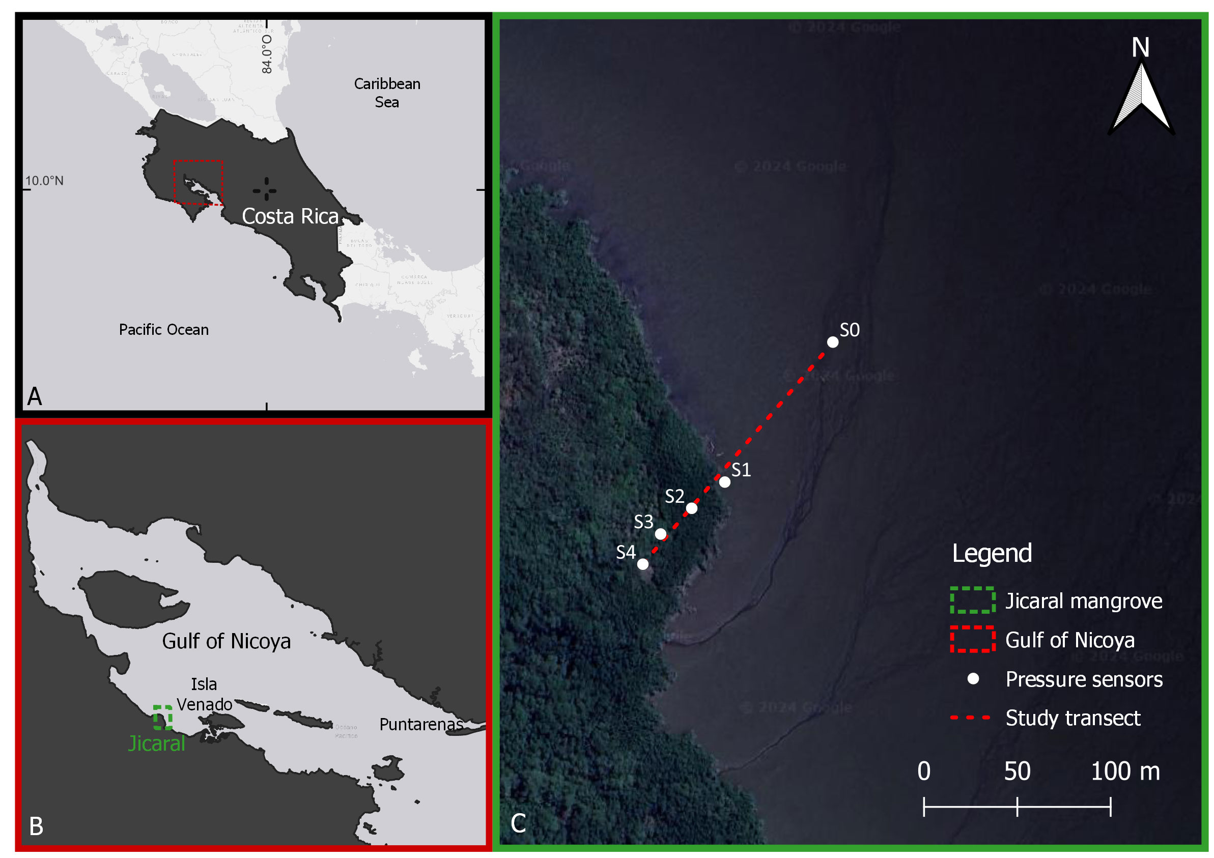
Figure 1 Study area. (A) Costa Rica is surrounded by the Caribbean Sea and Pacific Ocean, and the location of the Gulf of Nicoya is indicated by the red rectangle. (B) Gulf of Nicoya with the Jicaral mangrove forest indicated by the green rectangle. (C) Study transect (red dashed line) and location of the RBR pressure sensors (white dots: S0, S1, S2, S3 and S4). (Map data: Google, Images © 2024 Airbus, CNES /Airbus, Maxar Technologies, Data Maps © 2024).

The Gulf of Nicoya is characterized by semidiurnal tides with tidal ranges of approximately 1.8 m during neap tides and up to 2.8 m during spring tides (Sibaja-Cordero and Gómez-Ramírez, 2022). Since the Gulf of Nicoya is sheltered from swells coming from the southwest and north Pacific, the largest waves in the area are generated by local winds. Therefore, the largest local waves are expected to occur from November to April, which originate from the northeast due to the intensification of trade winds (Lizano, 2007).

A transect of 163 m was established in the Jicaral mangrove forest (Figure 1C) based on the greatest fetch affecting the study area according to the predominant wind direction reported by Lizano (2007). Five RBRsolo³D|wave16 pressure sensors were deployed along the transect (S0, S1, S2, S3 and S4), as shown in Figure 1C. To characterize the wave evolution in the nonvegetated area, S0 sensor was deployed 100 m offshore from the S1 sensor, which was located at the leading edge of the mangrove forest. The first 100 m of the study transect covered the mudflat zone, which had a mean bottom slope of 2.7:1000. The remaining 63 m consisted of a vegetated zone with a mean bottom slope of 9.3:1000 that was covered by Rhizophora mangle forest.

2.1.2 Data collection and processing

The field campaign was conducted from February 20 to March 13, 2022. During this period, four visits were made to the mangrove forest to deploy the instruments, measure the bed level elevation and characterize the mangrove trees along the study transect. These visits were scheduled during ebb tide periods.

2.1.2.1 Bed level elevation survey

Figure 2A shows the bed level along the study transect and the location of the pressure sensors. A topographic survey was conducted using the real-time kinematic technique based on reference point IV-01 previously established in Isla Venado by the Coastal, Rivers and Estuaries Engineering Unit (IMARES) of the University of Costa Rica. A pressure sensor was used to measure the tide level variation to compare the vertical coordinate with the Puntarenas tide gauge record and to provide the reference level with respect to the mean of the lowest spring tide levels.

Figure 2

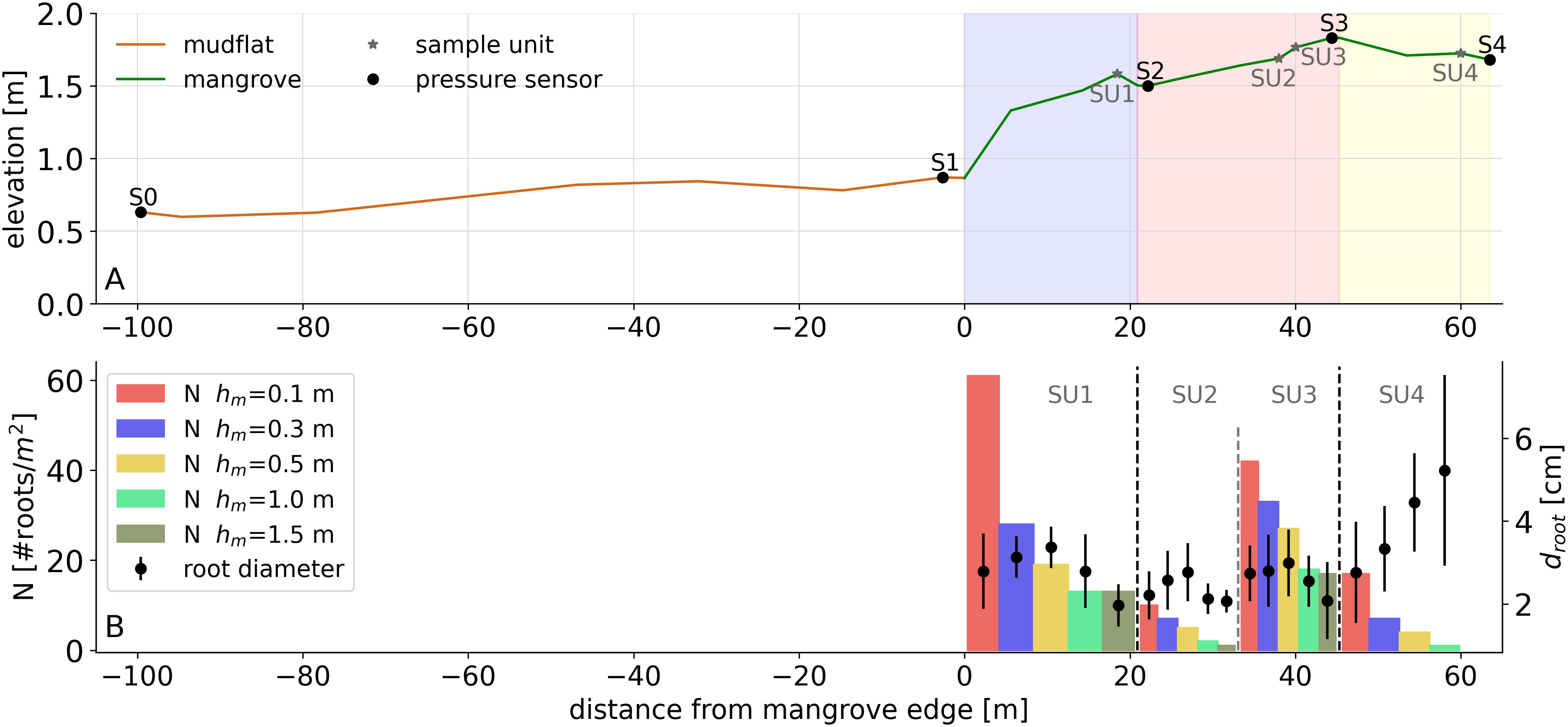
Figure 2 (A) Bed-level elevation of the study transect. The mudflat zone is indicated by the continuous brown line, and the mangrove forest is indicated by the continuous green line. Zone 1 corresponds to the light blue section, Zone 2 to the light red section and Zone 3 to the yellow section. S0-S4 refer to the locations of the pressure sensors, and SU1-SU4 refer to the sample units where the mangrove forest is characterized. (B) Vertical variation in the number of roots per m² ($N$) for each SU, values for $h_m$ between 0-0.1 m are indicated by the red bar, by the purple bar between 0.1-0.3 m, by the yellow bar between 0.3-0.5 m, by the green bar between 0.5-1.0 m and by the dark green bar for values greater than 1.0 m. The markers with error bars indicate the mean root diameter ($d_{root}$) with its respective standard deviation.

2.1.2.2 Vegetation survey

The mangrove species found in Jicaral was the Rhizophora mangle. In field, muddy areas in front and within the mangrove forest, composed of silty and clayey sediment, were observed. As reported by Jiménez (1999), this species occupies silty-clayey areas and has a poorly developed structure within the Gulf of Nicoya. This particular structure makes it difficult to distinguish between its stem and aerial roots because of its prostrate habit, as described by Jiménez and Soto (1985) (Figure 3). Mangrove tree characterization was conducted along the 63 m transect of the mangrove forest. The transect was divided into three distinct zones based on tree density (Figure 2A). Zone 1 corresponded to the first 21 m, Zone 2 covered the subsequent 24 m, and Zone 3 covered the following 18 m. Due to the difficulty of accessibility and movement through the forest, as well as the time constraints imposed by the advancing tide, 2 × 2 m area units were sampled to characterize the mangrove trees in each zone. A total of 4 sampling units (SUs) were strategically distributed to capture the variability in mangrove root density ($N$) and root diameter ($d_{root}$) (Figure 2B). Specifically, one sampling unit (SU1) constituted Zone 1, Zone 2 was characterized by two sampling units (SU2 and SU3), which were intended to capture low- and high-density areas present within that zone, and Zone 3 constituted one sampling unit (SU4). For low-density zones (SU2 and SU4), 100% of the 2 × 2 m area was sampled (Figure 3A), whereas for high-density areas, 25% of the SU area was randomly sampled; these areas were considered to be representative of the entire 4 m² area (Figure 3B). The $N$ and $d_{root}$ measurements were taken at 0.1, 0.3, 0.5, 1 and 1.5 m above ground (Figure 3C) to ensure that the complex root system structure spanning the height of the mangrove was represented accurately.

Figure 3

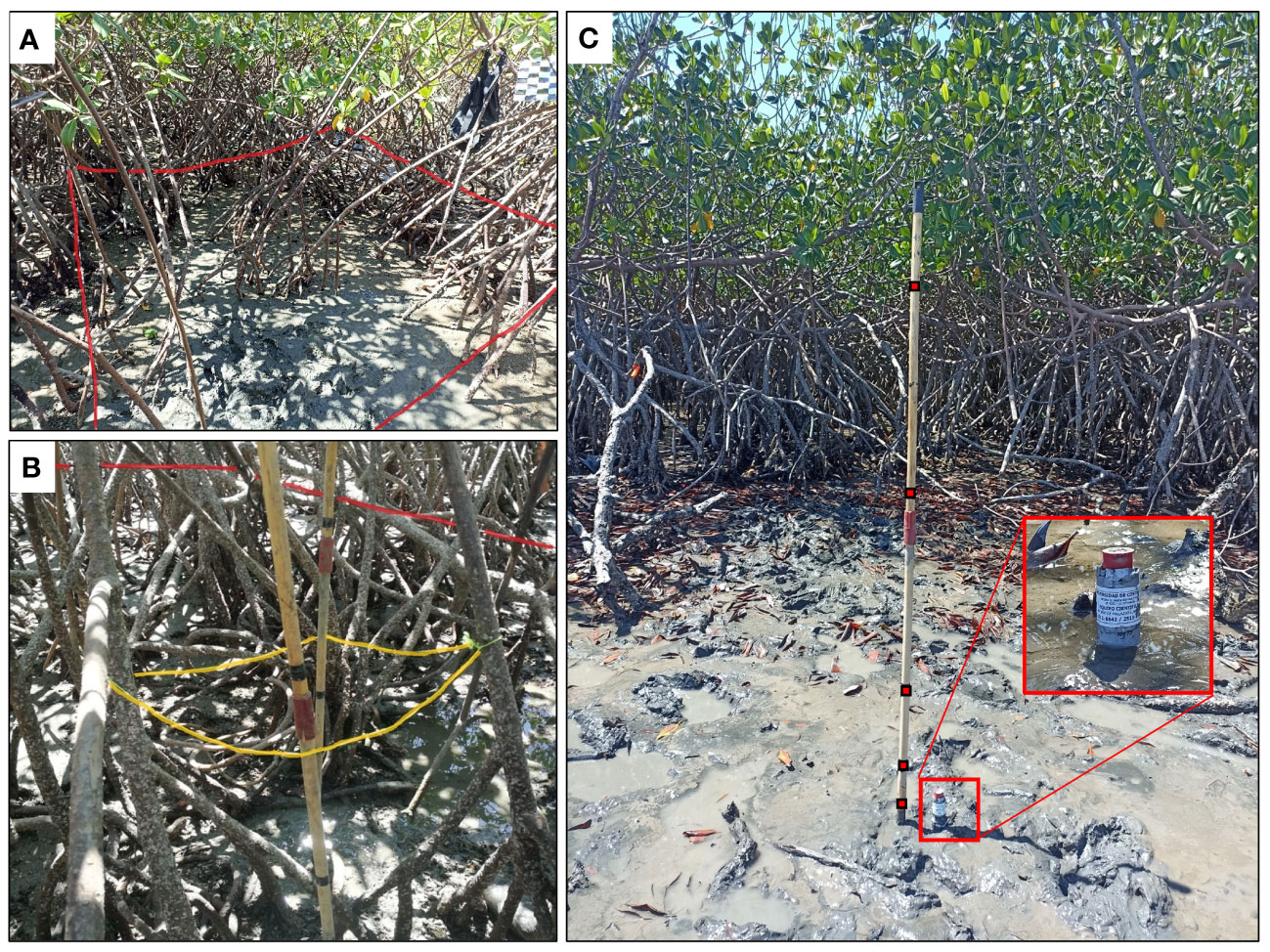
Figure 3 (A) Sampling unit SU2 (example of SU for low-density areas); a 2x2 m sample area is delimited by the red line. (B) Sampling unit SU1 (example of SU for high-density areas); 25% of the total 2x2 m area is delimited by the yellow line. (C) Reference used for measuring root diameters at distinct elevations above the bed (red marks at 0.1, 0.3, 0.5, 1, and 1.5 m from the bed level) and pressure sensor S1 located at the leading edge of the mangrove forest (red rectangle).

Zone 1 had the highest density, with 61 roots/m² at a height of 10 cm above the ground; this density decreased by 78% at a height greater than 1 m, with 13 roots/m² (Figure 2B). Zone 2 included areas with both high and low root densities. They encompass areas with low density (SU2), 10 roots/m² at a height of 10 cm, and areas with densities up to 42 roots/m² at a height of 10 cm (SU3). Finally, Zone 3 had a lower root density than the other two zones, with a density of 17 roots/m² at a height of 10 cm. SU1, SU2 and SU3 exhibited similar $d_{root}$ values, with the highest diameter values occurring at 30 and 50 cm above the ground (Figure 2B). Conversely, for SU4, $d_{root}$ tends to increase slightly as the measurement point moves away from the ground, exceeding 4 cm in diameter for heights of 1 m. Additionally, SU4 has the greatest variability, with standard deviations exceeding 1 cm. This variability may be attributed to changes in environmental factors, e.g., substrate consolidation and wave and wind exposure, since these areas are located in the inner parts of the forest. Variations in density across the zones are also reported in Supplementary Table 1.

2.1.2.3 Hydrodynamic data collection and postprocessing

Five RBR pressure sensors were deployed to capture the wave height evolution in the mangrove forest. The sensors have a nominal accuracy of 0.01 m and a resolution< 0.0002 m according to the manufacturer. These sensors were secured inside a fixed PVC structure buried in the ground (red rectangle in Figure 3C). During the sampling time, several visits to the mangrove forest were made to clean the pressure sensors to prevent any blockage due to sediment accumulation. These sensors recorded pressure variations every 20 min, and 8192 measurements per burst were recorded, i.e., approximately 8.5 min at a sampling frequency of 16 Hz. The devices were positioned between 2 and 17 cm above the bed level, with an average height of 8 cm. The distances between the sensors in the transects are shown in Table 1. The sensor spacing approximately corresponded to the mangrove forest density zoning (Figure 2A).

Table 1

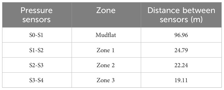
Table 1 Distance between pressure sensors and their corresponding zone based on root density.

To postprocess the pressure data, first, an atmospheric pressure correction was applied. The correction was based on the atmospheric pressure measured by the sensor during low tide conditions at the site. Subsequently, the hydrostatic pressure and dynamic wave pressure signals were extracted. The mean water level was considered to be the one associated with the mean pressure recorded in each burst. To obtain the dynamic pressure, linear detrending was performed for each burst to subtract the tidal effect. In addition, a depth attenuation correction was conducted for frequencies ranging between 0.05 Hz and 0.43 Hz with a maximum correction factor of 5 to avoid overamplification of high-frequency signals, as described by Hu et al. (2021). Finally, following the methods employed in other studies (e.g., Horstman et al., 2014; Best et al., 2022), a spectral analysis was conducted to obtain parameters, such as the significant wave height ($H_{m0}$) and peak period ($T_p$). To ensure an adequate characterization of the wave height evolution in the mangrove forest, bursts in which all the sensors were inundated and $H_{m0}$ exceeded 0.05 m at S1 were selected following Quartel et al. (2007).

2.2 Quantification and simulation of wave height attenuation

Two approaches are used for quantifying wave height attenuation in the Jicaral mangrove forest: the wave height attenuation rate ($r$) and the drag force approach, which are widely used in numerical models, including the Simulating Waves nearshore (SWAN) model (Booij et al., 1999). The first approach is used to evaluate the correlation between water depth ($h$) and $H_{m0}$ with the $r$ values for the mudflat zone and the mangrove zone. In contrast, the drag force approach is used to obtain an adequate estimation of ${\tilde{C}}_D$ in the field, which will be useful for later numerical models based on this approach (Mendez and Losada, 2004).

2.2.1 Wave height attenuation rate

Previous field campaign studies (e.g., Mazda et al., 1997a, Mazda et al., 2006; Quartel et al., 2007; Horstman et al., 2014; Zhou et al., 2022) used the rate of wave height attenuation per unit distance, Equation 1, to characterize wave attenuation due to vegetation and bottom friction.

$\begin{array}{ll}r=-\frac{\Delta H}{H_i}·\frac{1}{\Delta x}& (1)\end{array}$

where $H_i$ is the incident wave height defined at the leading edge of the mangrove forest and $\Delta H$ is the difference between the wave heights at distance $\Delta x$. This parameter is widely used to quantify the variation in wave height per linear meter in a forest. Studies, such as Horstman et al. (2014), have related this parameter to vegetation density. Instead, Zhou et al. (2022) used the approach of Mazda et al. (1997a), which does not consider vegetation characteristics to be related to ${\tilde{C}}_D$ and $r$, as discussed later in section 4.4. This study used this approach to quantify the wave height evolution in mangrove forests and to compare the results with those of other studies conducted at other sites worldwide. Furthermore, the calculated values are correlated with parameters, including $H_{m0}$ and $h$.

2.2.2 Drag force approach: wave damping coefficient

Dalrymple et al. (1984) developed a model based on the work done to vegetation by the drag force to describe the wave height evolution of regular waves along the vegetation field. Mendez and Losada (2004) extended this model to include random waves, and Equation 2 is the analytical solution.

$\begin{array}{ll}{H}_{rms}=\frac{H_{rms,0}}{1+ \beta x}& (2)\end{array}$

where $H_{rms}$ is the root mean square wave height, x is the position along the vegetation field, being x=0 at the leading edge of the forest, subscript 0 indicates the incident value, and $\beta$ is the wave damping coefficient given by the following expression:

$\begin{array}{ll} \beta = \frac{{\tilde{C}}_D d_{root} N k H_{rms,0} }{3 \sqrt{\pi } } \frac{{\sinh }^{3}k{h}_v+3 \sinh k{h}_v }{(\sinh 2kh+2kh) \sinh kh}& (3)\end{array}$

where $h_v$ is the submerged height of mangrove $$ and $k$ is the wave number.

Suzuki et al. (2012) implemented the Mendez and Losada (2004) equation, Equations 2 and 3, in the third-generation full spectrum SWAN model and included the vertical and horizontal variations in vegetation characteristics in the model. Therefore, the results from the detailed geometric characterization of the mangrove forest described in Section 2.1.2.2 were used in the SWAN model to compute the wave height dissipation. The frontal area per unit height per square meter ($A_{hm}$) is obtained as a function of $N$ and $d_{root}$ by assuming a cylindrical geometry of the roots along the mangrove tree. To include $A_{hm}$ vertical variations in the SWAN model, an $A_{hm,j}$ value for each vertical layer $j$ was computed for each mangrove zone. Due to the limitations of the SWAN model when the vertical and horizontal geometries of mangrove forests are introduced simultaneously, the vertical variation in tree structure in Zone 1 is considered to be a reference for the horizontal distribution of mangrove features throughout the forest. The tree structure in Zones 2 and 3 is determined as a function of the tree characteristics in Zone 1 multiplied by a factor ${\alpha }_{zone2}$ for Zone 2 and ${\alpha }_{zone3}$ for Zone 3. These factors correspond to the mean ratio between $A_{hm}$ for Zone 2 $(A_{hm\_zone2})$ or Zone 3 $(A_{hm\_zone3})$ and $A_{hm}$ for Zone 1 $(A_{hm\_zone1})$, which include all the $n$ vertical layers considered, Equations 4, 5.

$\begin{array}{ll}{\alpha }_{zone2}=\left({\displaystyle \sum _{j=1}^n\frac{A_{hm\_zone2,j}}{A_{hm\_zone1,j}}}\right)\frac{1}{n} & (4)\end{array}$

$\begin{array}{ll}{\alpha }_{zone3}=\left({\displaystyle \sum _{j=1}^n\frac{A_{hm\_zone3,j}}{A_{hm\_zone1,j}}}\right)\frac{1}{n} & (5)\end{array}$

Then, the $A_{hm}$ values for each vertical layer in Zone 2 and Zone 3 are given by Equations 6 and 7, respectively:

$\begin{array}{ll}{A}_{hm\_zone2,j}=A_{hm\_zone1,j} {\alpha }_{zone2}& (6)\end{array}$

$\begin{array}{ll}{A}_{hm\_zone3,j}=A_{hm\_zone1,j} {\alpha }_{zone3}& (7)\end{array}$

Once the mangrove forest characteristics are known (Supplementary Table 2), the numerical model setup is defined considering a 1D scheme since the bathymetry of the Jicaral mangrove corresponds to the transect defined in Figure 2. This bathymetry is included and has a resolution of 0.5 m. To reproduce bottom friction under field conditions, wave height attenuation along the mudflat (between sensors S0 and S1) is considered to calibrate the Nikuradse roughness length scale using SWAN. In this case, the mean value obtained is 0.026 m, which is mainly attributed to the shape of the small wave ripple found in situ. This value agrees with the those reported by Van Der Lee (1998) (0.02 and 0.03 m) for tidal flats with small wave ripples. The Battjes and Janssen (1978) model with a wave breaking parameter of 0.73 is also used. Finally, the wave inputs correspond to $H_{m0}$ and the mean wave period ($T_{m01}$) measured at sensor S1, assuming a JONSWAP spectrum. ${\tilde{C}}_D$ is calibrated by determining the value that best fits the modeled wave height with the measured wave height through the forest, similar to the methodology used in previous studies under laboratory conditions for other trees (e.g., Kalloe et al., 2022; van Wesenbeeck et al., 2022). The refined Willmott’s index of agreement (Willmott et al., 2012), $d_r$, is used to select the ${\tilde{C}}_D$ value that best fits the wave height decay measured in the field for each case. When $d_r$ values are close to 1, it indicates a very good agreement between the model data and field measurements. Cases with $d_r$ greater than 0.9 are chosen as the best ${\tilde{C}}_D$ representative values for reproducing the wave height decay produced by the mangrove forest. These resultant ${\tilde{C}}_D$ values are related to their respective $KC$ number to obtain a predictive ${\tilde{C}}_D$ formulation. Several authors have demonstrated a high correlation between ${\tilde{C}}_D$ and $KC$ (e.g., Ozeren et al., 2014; Cao et al., 2016) leading to formulations that allow estimating ${\tilde{C}}_D$ as a function of $KC$. $KC$ is defined by considering mangrove characteristics and the incident hydrodynamic conditions to which they are exposed, resulting in a predictable parameter that can subsequently be related to ${\tilde{C}}_D$. Following this approach, the $KC$ number is given by Equation 8:

$\begin{array}{ll}\text{KC}=\frac{u_c T_p}{d_{root}}& (8)\end{array}$

where mean $d_{root}$ measured in the field (2.88 cm) is used as the characteristic length scale. The complex geometry of Rhizophora mangle trees, in which roots and trunks are difficult to differentiate because of the prostrate growth characteristic of this species, causes $d_{root}$ to be the best geometrical value representing the interaction of the waves with these trees. Using linear theory, the depth-averaged velocity, $u_c$, is considered to be the characteristic velocity and it is calculated based on the average water depth between S1 and S4, together with $H_{m0}$ and $T_p$ measured at S1.

3 Results

3.1 Wave conditions

Figure 4 shows $H_{m0}$, $T_p$, $h$ and relative wave height ($H_{m0}/h$) values for the bursts in which all the sensors are inundated and $H_{m0}$ in S1 is greater than 0.05 m. The recorded $H_{m0}$ values during the measurement period did not exceed 0.38 m (Figure 4A). The $T_p$ values ranged from 1.88 to 3.76 s (Figure 4B), and the maximum $h$ value recorded at sensor S1 during spring tides was 2.38 m (Figure 4C). The relative wave heights did not exceed 0.36 (Figure 4D), suggesting that wave breaking is not the main wave dissipation mechanism since wave breaking occurs when wave heights exceed 60% of $h$ (Horstman et al., 2014; Cao et al., 2016).

Figure 4

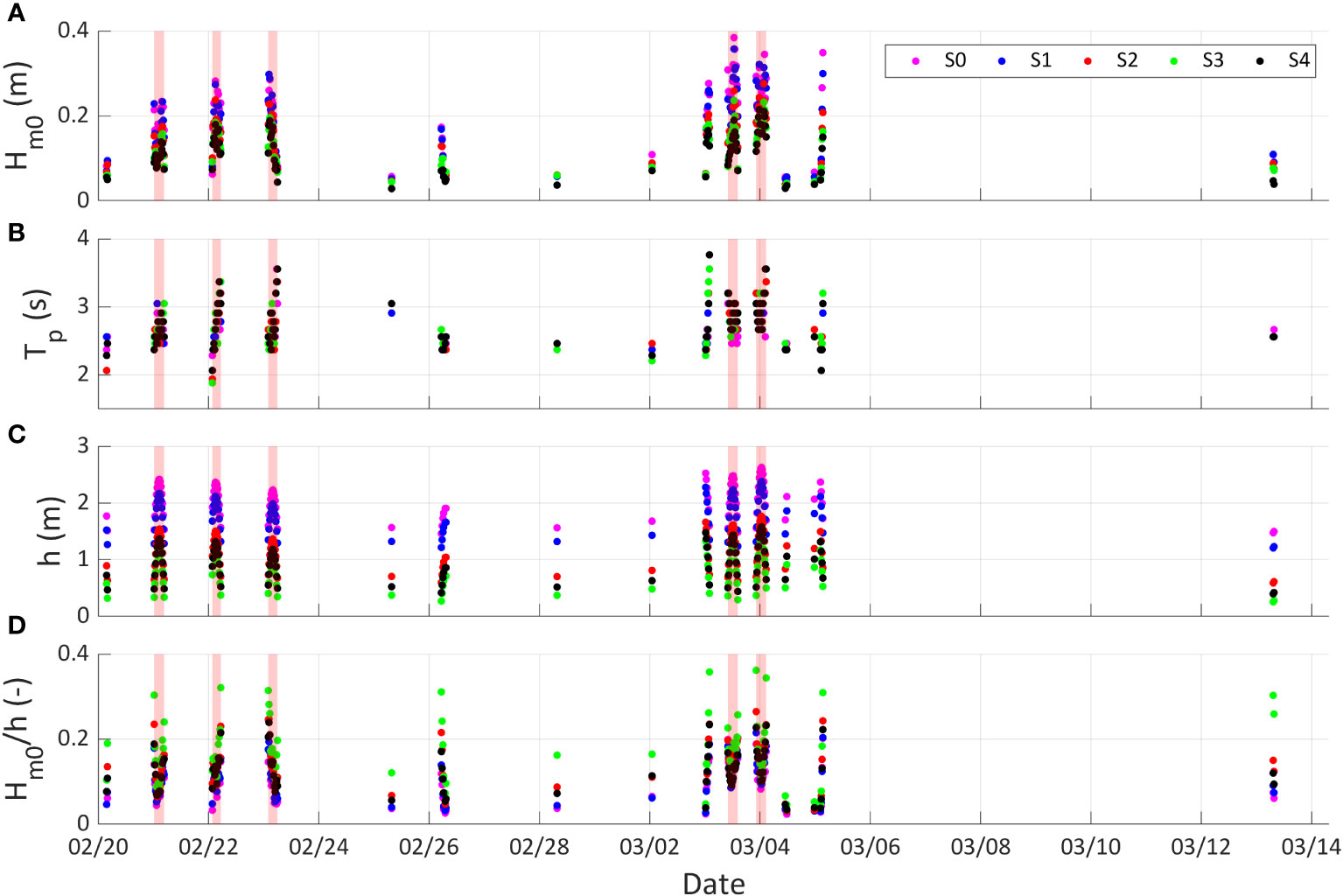
Figure 4 Hydrodynamic conditions measured in the field from February 20 to March 13. Time series of (A) significant spectral wave height ($H_{m0}$), (B) peak period ($T_p$), (C) water depth ($h$) and (D) relative wave height ($H_{m0}/h$) are shown for the different pressure sensors: S0 (magenta circles), S1 (blue circles), S2 (red circles), S3 (green circles) and S4 (black circles). The 5 largest tides are indicated in red.

Figure 5 displays the time-averaged spectral densities for the bursts corresponding to the five largest tides with $h$ values exceeding 2 m, which are highlighted in red in Figure 4. The selected bursts include the tides for February 21 (Figure 5A), February 22 (Figure 5B), February 23 (Figure 5C) and March 4 at 2:00 and 16:00, corresponding to Figures 5D and E, respectively. The observed spectra are unimodal, with wave periods ranging from approximately 2.2 to 4 s, which are typical of local waves generated by winds, suggesting no presence of infra-gravity waves. The most energetic incident waves were recorded at sensor S1 on March 4, with maximum energy densities twice as high as those recorded in February.

Figure 5

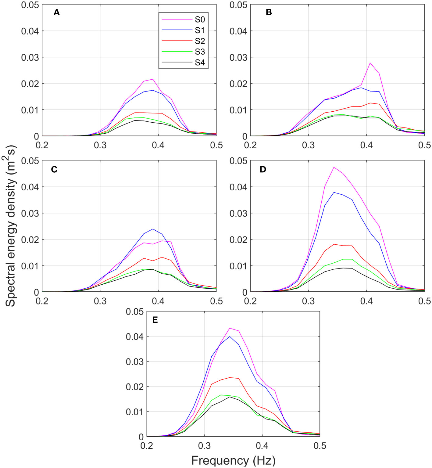
Figure 5 Time-averaged spectral energy densities for the 5 largest tides for the different pressure sensors deployed along the transect: S0 (magenta line), S1 (blue line), S2 (red line), S3 (green line) and S4 (black line). The selected tides are those recorded on (A) February 21, (B) February 2, (C) February 23, (D) March 4 at 2:00 and (E) March 4 at 16:00.

The results indicate that the maximum energy density decreases by an average of 20% in the mudflat region between sensors S0 and S1, except for the spring tide case on February 23, where a slight increase in energy is recorded at S1. This increase may be attributed to local effects, such as wind-induced energy. The greatest reduction occurs along the first 24.8 m of the forest between sensors S1 and S2, with the maximum energy density decreasing by 40% on average. Conversely, for the last section of the mangrove plant, between S3 and S4, the energy dissipation is the lowest, with the maximum energy density decreasing by an average of 10%. This decrease in energy density reduction is expected due to a decrease in both mangrove forest density and wave height. In general, as waves propagate through mangroves (S1–S4), there is a notable decrease in energy density. The wave height is reduced by 34% on average, similar to the value estimated by Maza et al. (2021) for a 35-year-old Rhizophora sp. forest with the same width as the Jicaral forest and a water depth equal to 2 m.

3.2 Wave height attenuation rates

Wave height attenuation rates are estimated by using Equation 1, where $r$ denotes the wave attenuation per linear meter. Figure 6 displays the $r$ values obtained between sensors S1 and S4 (mangrove zone, black dots) and sensors S0 and S1 (mudflat zone, red dots) for each recorded burst as a function of the measured water level at S1. The black and red lines represent the linear fits of the data for the mangrove and mudflat zones, respectively. Within the mangrove forest, wave attenuation tends to decrease as water depth increases, as indicated by the black line. A similar trend was reported by Mazda et al. (1997a) and Mazda et al. (2006) in Kandelia candel and Sonneratia sp. forests. In addition, Figure 6 shows that the $r$ values in the mudflat zone tend to be constant independent of water depth.

Figure 6

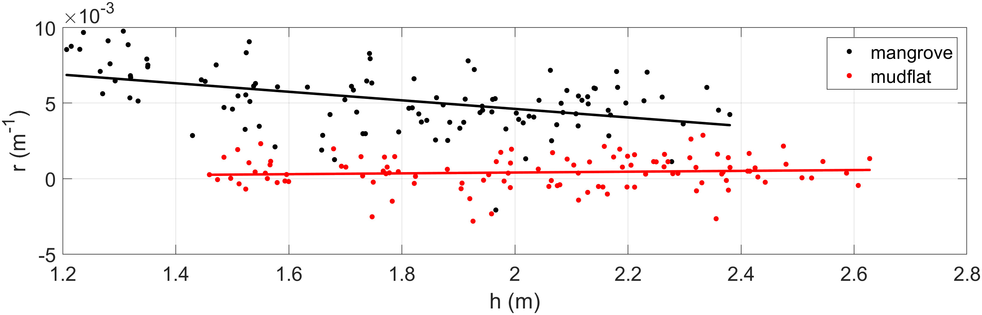
Figure 6 Wave attenuation rate ($r$) as a function of water depth ($h$). The $r$ values for the mangrove forest zone are represented by black dots, and those for the mudflat zone are represented by red dots. Continuous lines indicate the best linear fit of $r$ as a function of $h$ for the mangrove (black line) and mudflat (red line) zones.

Figure 7 shows $r$ as a function of the incident wave height. As shown, as $H_{m0}$ increases, the wave attenuation also increases, as reported by Horstman et al. (2014). In contrast, in the mudflat, there is also no clear variation trend for $r$ with respect to $H_{m0}$, and in some cases, there is an increase in the wave height between sensors S0 and S1, which agrees with Figure 5C.

Figure 7

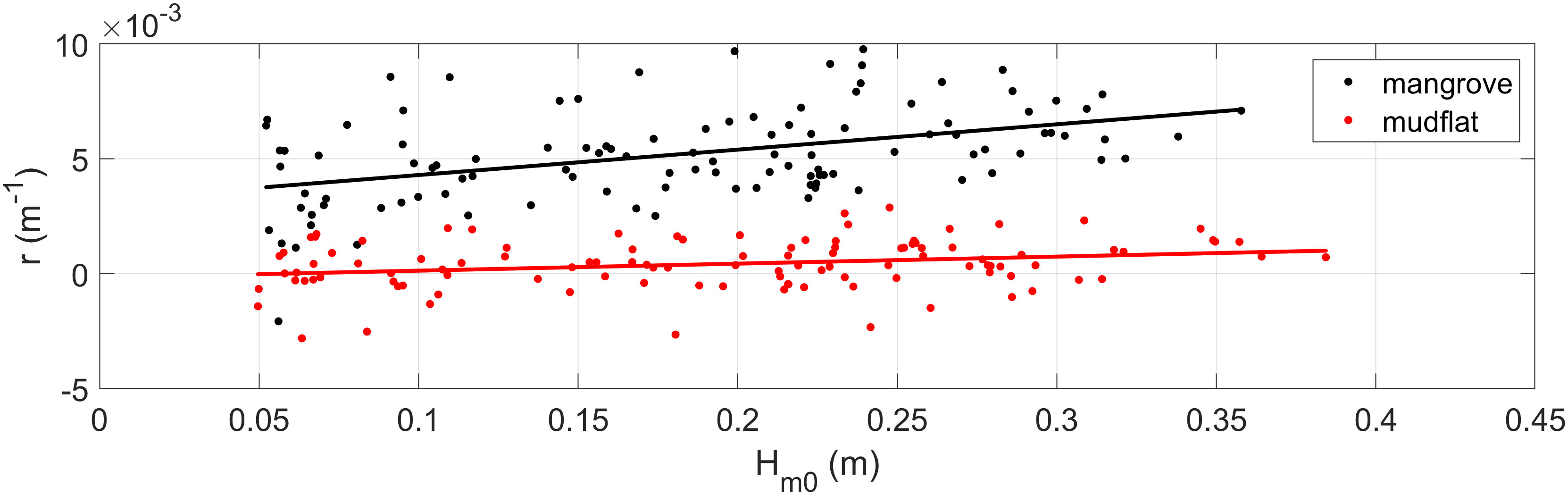
Figure 7 Variation in the wave attenuation rate ($r$) for different $H_{m0}$ values. The $r$ values for the mangrove forest (black dots) and mudflat zone (red dots) and their respective linear fits, as a function of $H_{m0}$, are indicated for the mangrove (black line) and mudflat (red line) zones.

In general, Figures 6, 7 present $r$ values in the mangrove field that vary between 0.001 and 0.01 m^-1, whereas those related to the mudflat zone tend to be one order of magnitude lower (10^-4) than those for the mangrove forest, with a mean value of 0.0004 m^-1. This difference suggests that the decrease in wave height along the forest is mainly attributed to the drag exerted by the trees, as demonstrated by previous studies (e.g., Mazda et al., 1997a; Horstman et al., 2014).

3.3 Vegetation properties along a Rhizophora mangle forest

Adequate characterization of mangrove tree structure is essential for modeling wave-vegetation interactions and identifying mangrove tree parameters, i.e., characteristic length, that better describe wave attenuation. Hence, this study represents the vertical and spatial variation in mangrove tree characteristics by $A_{hm}$, calculated from the variables $N$ and $d_{root}$. Figure 8 displays $A_{hm}$ values for different elevations above the ground ($h_m$), where the blue line corresponds to the $A_{hm}$ vertical variation in Zone 1, the red line is for Zone 2 and the green line is for Zone 3. For Zone 2, the characteristics reported in Figure 2B for both SU2 and SU3 were averaged, because based on visual inspection in the field, both sample units represented areas equally distributed along the transect. Zone 1 presented the largest $A_{hm}$ values, which were reduced by 60% and 73% in Zone 2 and Zone 3, respectively, for $h_m$ =10 cm. Instead, as $h_m$ increases, the $A_{hm}$ differences between zones decrease, revealing the influence of secondary roots on low $h_m$ values.

Figure 8

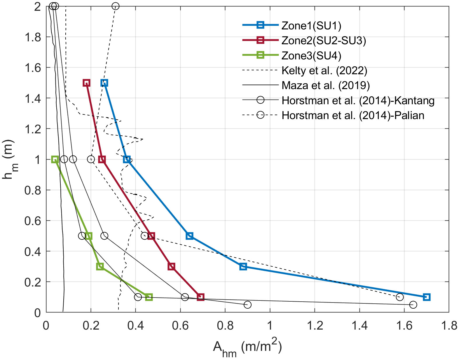
Figure 8 Frontal area per unit height per square meter ($A_{hm}$) for different elevations above the bed ($h_m$) obtained from the Jicaral mangrove forest. Zone 1 corresponds to the blue line, Zone 2 corresponds to the red line and Zone 3 corresponds to the green line. $A_{hm}$values reported in laboratory studies, such as Kelty et al. (2022) (dashed black line) and Maza et al. (2019) (continuous black line) are shown for different $h_m$ values. Variations in $A_{hm}$with respect to $h_m$ in the field, as reported by Horstman et al. (2014) for Rhizophora sp., is presented for Kantang (continuous line with circle markers) and Palian (dashed line with circle markers).

In addition to the data collected in Jicaral, Figure 8 shows the $A_{hm}$ values of previous studies that have measured or parameterized mangrove geometry for Rhizophora sp., either in the field or laboratory. A detailed characterization of a mangrove forest at two sites, Kantang and Palian, which were monitored in Thailand and reported by Horstman et al. (2014), is included. Specifically, the data correspond to the areas where Rhizophora sp. trees are predominant. For Kantang, the calculated $A_{hm}$ values at a height of 10 cm are similar to those obtained for Zone 2 and Zone 3 at a height of 10 cm above the ground. At 5 cm, the presence of pneumatophores from Avicennia/Sonneratia trees causes $A_{hm}$ to increase considerably and become similar to those found in Zone 1 at a height of 10 cm, revealing the high density of roots in the Jicaral mangrove at the leading edge. Additionally, the vertical distributions of $A_{hm}$, reported by Maza et al. (2019) and Kelty et al. (2022), are included in Figure 8. In both studies, laboratory tests were conducted to quantify wave attenuation in a mangrove forest. The forests were constructed using mangrove tree representations, which were defined based on Ohira et al. (2013) parametrization for Rhizophora sp. trees. Due to the low tree density (0.0625 trees/m²) considered in the experiments of Maza et al. (2019), low $A_{hm}$ values are obtained compared to the data collected in Jicaral. On the other hand, Kelty et al. (2022) based their parametrization on mangrove measurements made in the Pacific of Costa Rica (Loría-Naranjo et al., 2014) where Jicaral is located, resulting in $A_{hm}$ values similar to those reported for Zones 1 and 2 for $h_m$ values greater than 0.5 m. Nevertheless, $A_{hm}$ values for $h_m$ = 0.5 m or less are lower than the $A_{hm}$ values measured in the field. This difference may be due to the use of the Ohira et al. (2013) parameterization, which considers only primary roots. The secondary and subsequent roots, which are primarily present at low $h_m$ values, are not considered. These roots may contribute up to 80% of the frontal area, as evidenced in the study by Yoshikai et al. (2021). Therefore, the role of stilt roots is essential for the wave damping capacity of Rhizophora trees.

3.4 Bulk drag coefficient for Rhizophora sp.

Most of the models developed to obtain wave height attenuation by vegetation rely on the adequate estimation of ${\tilde{C}}_D$. It is necessary to develop a ${\tilde{C}}_D$ formulation that considers the variation in mangrove forest characteristics and wave field conditions. Thus, field conditions are simulated using the SWAN model to obtain calibrated ${\tilde{C}}_D$ values. Figure 9 shows an example of six simulated cases, including the variation in the mangrove forest in the field and considering different wave conditions. The SWAN results are represented by continuous lines, whereas the field measurements are represented by dots. The error bars in Figure 9 indicate the variation in the SWAN results if the standard deviation of $d_{root}$ (Supplementary Table 1) is considered, following the methodology presented in section 2.2.2. In Zone 1, a maximum $H_{m0}$ difference of 8.4% and a minimum value of 3.5% with respect to the mean value are found when comparing the SWAN results using the $d_{root}$ mean value with those using the upper and lower limits. However, in Zone 3, the maximum difference is 17.2% (Figure 9D), and a minimum value of 7.38% is found (Figure 9A). The cases represented in Figures 9D, E exhibit higher variability using the lower and upper limits of $d_{root}$ along the transect. These cases correspond to the highest incident wave heights. This result indicates that a variation in the frontal area generates a greater change in energy dissipation in cases with high drag forces, i.e., high orbital velocities, than in cases where the wave height is lower and, consequently, the orbital velocities are also lower. The good agreement along the mangrove transect using a single ${\tilde{C}}_D$ value reveals that an adequate mangrove forest characterization that considers the spatial distribution of tree traits, combined with the varying velocity field affecting the forest, leads to a constant ${\tilde{C}}_D$ value across the forest, which agrees with the findings of Maza et al. (2017).

Figure 9

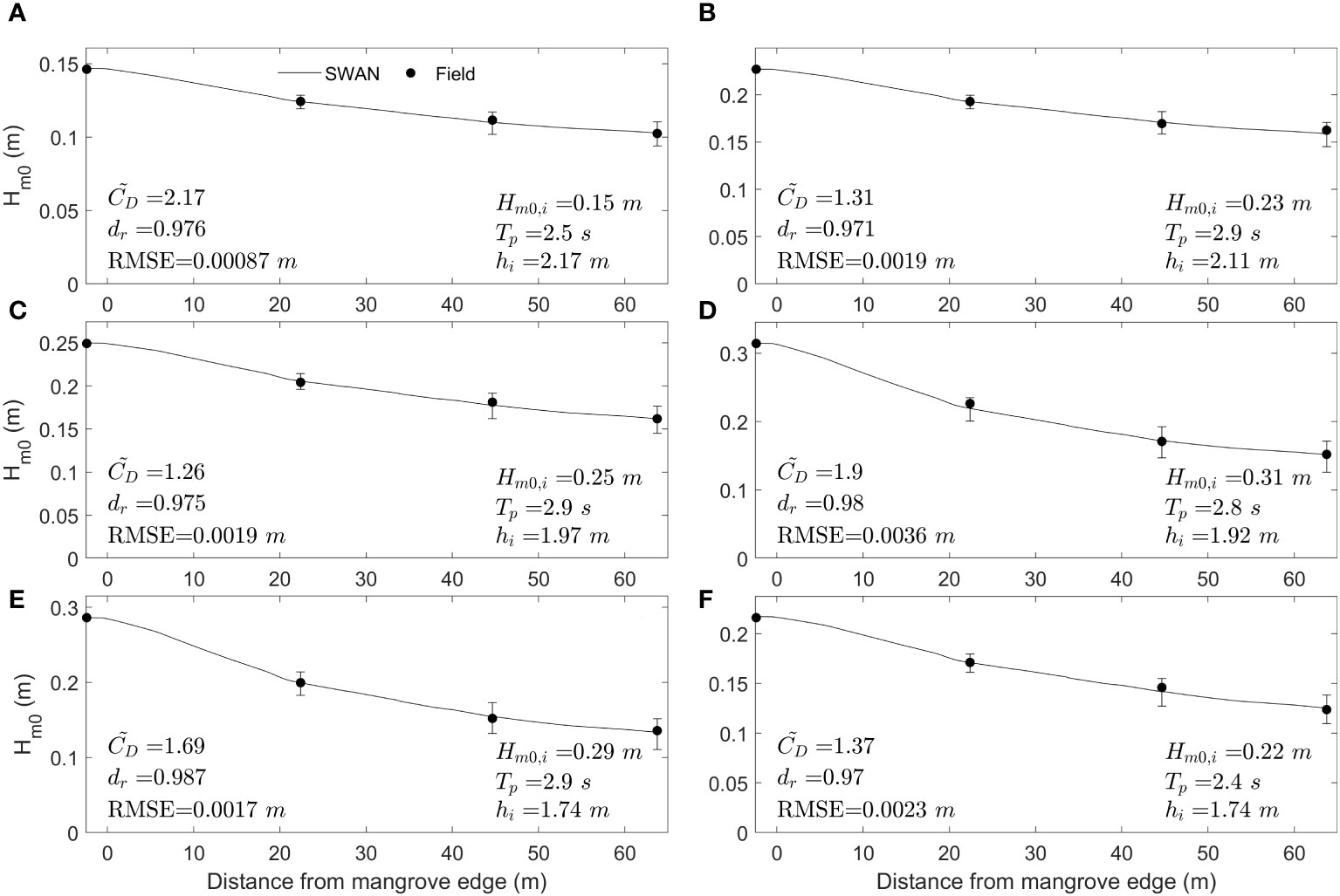
Figure 9 Results of the calibration between SWAN simulations (continuous line) and wave field measurements (black dots) with their respective calibrated Cd values for six cases with distinct incident wave conditions (A-F). The incident significant wave height ($H_{m0,i}$), peak period ($T_p$) and incident water depth ($h_i$) at sensor S1 are presented. In addition, the index of agreement ($d_r$) and root mean square error ($RMSE$) are shown for each calibrated case. The error bars indicate the results of the SWAN simulations if the standard deviation of the $d_{root}$ shown in Figure 2B is used.

The ${\tilde{C}}_D$ values that best represent the wave height attenuation in the mangrove forest are shown in Figure 10 with their respective $KC$ numbers with green dots. Furthermore, Maza et al. (2019) and Kelty et al. (2022) data for ${\tilde{C}}_D$ vs. $KC$ are included, purple and yellow dots respectively. These data are used because they tested Rhizophora sp. representations under random wave conditions, similar to the conditions found in the field. For consistency, the $d_{root}$ values reported by these two studies are also employed as the characteristic length scale in the $KC$ formula. By considering a common relationship that allows us to obtain ${\tilde{C}}_D$ as a function of $KC$, that is, by knowing the incident wave conditions and the characteristic diameter of the forest, the data in this study, combined with those from Maza et al. (2019) and Kelty et al. (2022), are fitted to an equation in the form of ${\tilde{C}}_D={(\frac{a}{KC})}^b+c$, resulting in Equation 9:

Figure 10

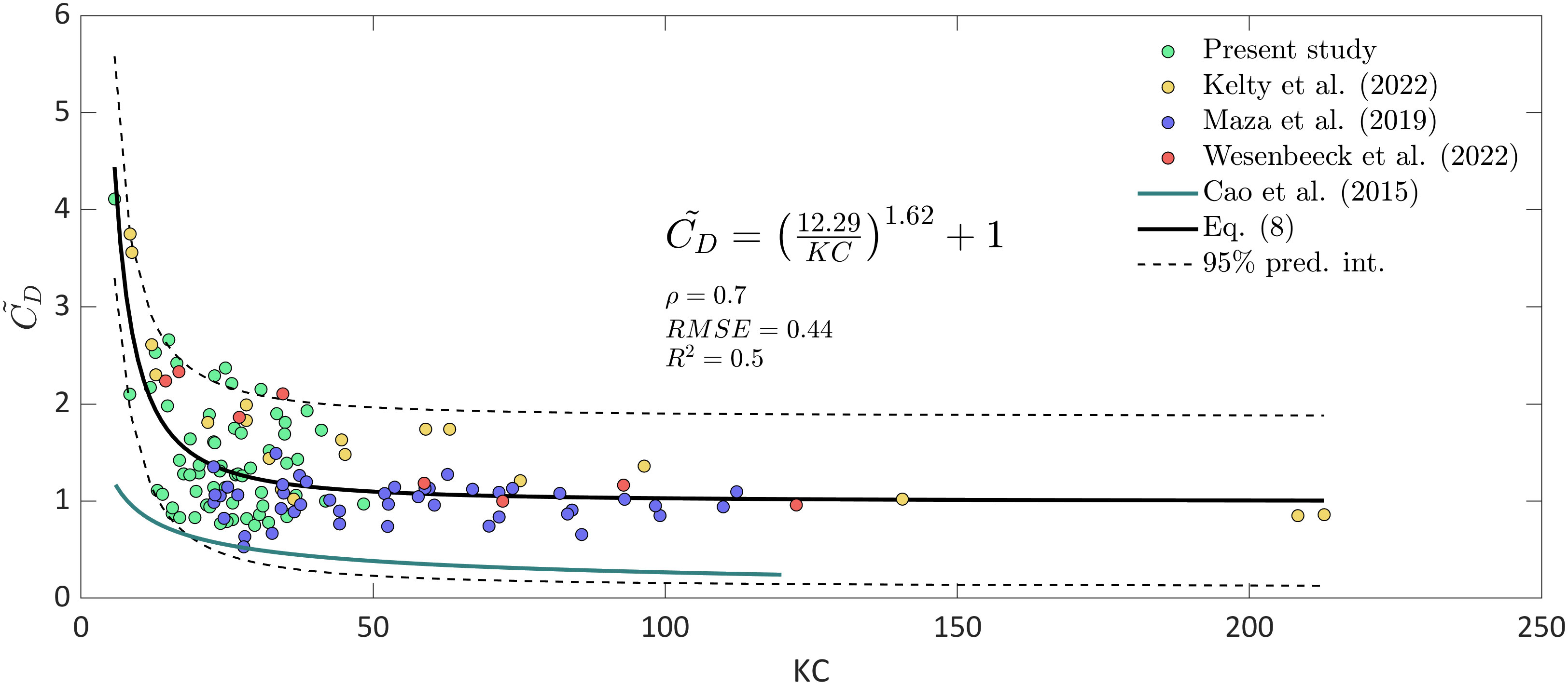
Figure 10 ${\tilde{C}}_D-KC$ relationships for Rhizophora sp. based on field and laboratory data (continuous black line) with the corresponding 95% prediction intervals (dashed lines). The obtained relationships include data from the present study (green dots), Kelty et al. (2022) (yellow dots) and Maza et al. (2019) (purple dots) for Rhizophora sp. Additionally, data from van Wesenbeeck et al. (2022), from their unique large-scale laboratory test with Salix alba trees (red dots), are included, and the ${\tilde{C}}_D-KC$ relationship for Avicennia marina reported by Cao et al. (2016) is also displayed (continuous light blue line).

$\begin{array}{ll}{\tilde{C}}_D={\left(\frac{12.29}{KC}\right)}^{1.62}+15.8<KC<212.8& (9)\end{array}$

The proposed ${\tilde{C}}_D$ equation based on $KC$ as a function of $d_{root}$ for Rhizophora sp. yields an acceptable result with a correlation coefficient ($\rho$) equal to 0.7, a root mean square error ($RMSE$) of 0.44 and a coefficient of determination ($R^2$) of 0.5 (Figure 10).

In addition, ${\tilde{C}}_D$ values from van Wesenbeeck et al. (2022) and Cao et al. (2016), obtained in the laboratory and field, respectively, are also included in Figure 10 to compare their results with those reported in this study. The values of ${\tilde{C}}_D$ are shown because they originate from woody vegetation but are not considered in Equation 9 since their geometric characteristics greatly differ from those of Rhizophora sp., leading to different wave-vegetation interaction patterns and, therefore, different drag force values. In the study by van Wesenbeeck et al. (2022), a unique large-scale laboratory experiment was conducted with woody vegetation, where the tested vegetation was pollard willow forest (Salix alba). They tested willows with full leaves and canopies, willows without leaves and full canopies, and willows without leaves and reduced canopies. Here, the cases in which the forest has all its leaves and full canopy are considered. In addition, the ${\tilde{C}}_D-KC$ relationship obtained by Cao et al. (2016) is also included as a continuous light blue line in Figure 10. The curve corresponds to Avicennia marina, which has a root system different than that of Rhizophora sp., and is mainly characterized by pneumatophores. Figure 10 reveals that the ${\tilde{C}}_D$ values found for Rhizophora sp. are similar to those produced by pollard willow despite the differences in their respective structures. Similarities in ${\tilde{C}}_D$ values are obtained predominantly for large $KC$ numbers when trees are exposed to greater wave hydrodynamics. However, further investigations are needed in these cases, when mangrove forests are exposed to high $KC$ numbers, i.e., extreme events. In contrast, Cao et al. (2016) reported low ${\tilde{C}}_D$ values compared to those in this study since, unlike Rhizophora sp., Avicennia marina presents pneumatophores as roots instead of as stilt roots. When the water depth exceeds the pneumatophore height (approximately 12 cm), the maximum orbital velocities are not directly affected by the pneumatophores, leading to less drag force and consequently lower ${\tilde{C}}_D$ values.

Equation 9 provides an estimate of ${\tilde{C}}_D$ for regions predominantly covered by Rhizophora sp. forest and affected mainly by shortwave conditions since the recorded field conditions do not include long waves (Figure 5). On the other hand, the influence of current tidal is explored by differentiating the ${\tilde{C}}_D$ values according to ebb or flood tidal cases (Supplementary Figure 1). The influence of tidal currents in ${\tilde{C}}_D-KC$ formulation is not evident; this may be attributed to low current velocities. Calleja et al. (2022) reported current tidal values below 0.025 m/s for the inner part of the Gulf and zones near to the coast when evaluating the suitability of aquaculture farms in the Gulf of Nicoya. The reported current velocities are lower than those from studies that have reported an influence of current in wave attenuation when interacting with waves and vegetation (e.g., Yin et al., 2020; Hu et al., 2021).

The proposed Equation 9 is obtained by combining laboratory and field data, resulting in an integrated ${\tilde{C}}_D$ formulation with $d_{root}$ as the characteristic length scale. To the best of our knowledge, this is the first attempt to combine laboratory and field data to develop a unique empirical equation ${\tilde{C}}_D$ for Rhizophora sp. forest.

4 Discussion

4.1 Detailed forest-scale characterization of mangrove trees

The estimation of wave height attenuation based on drag-force models requires the characterization of mangrove forests to determine the frontal area exposed to flow action. In the laboratory, great efforts have been made to represent and to characterize in detail artificial mangrove trees using techniques such as laser scanning and photogrammetry (e.g., Maza et al., 2019; Kelty et al., 2022). In the field, detailed trunk and root diameter measurements (e.g., Horstman et al., 2014; Zhou et al., 2022) are often performed at the forest scale to capture mangrove traits due to limitations in employing techniques used in laboratory. When measuring trunk and root diameters in the field, significant effort is required to obtain similar vertical resolution of the tree frontal area as in the laboratory. Nevertheless, the results obtained for $A_{hm}$ in the laboratory and the field are comparable (Figure 8). On the other hand, in the laboratory, the spatial heterogeneity of the frontal area along mangrove forests is not considered; in contrast to field studies, it is possible to capture the spatial variability in mangrove forest traits. The detailed mangrove forest characterization, as performed in Jicaral, allows for a reliable representation of field conditions while accounting for mangrove spatial distribution, which is essential for the adequate estimation of wave energy dissipation through the forest.

4.2 Root diameter determining Rhizophora sp. wave attenuation

To estimate ${\tilde{C}}_D$ as a function of vegetation properties, it is important to determine an appropriate characteristic length scale that represents mangrove geometry and how it influences flow conditions. For Rhizophora sp. under random wave conditions, Maza et al. (2019) and Kelty et al. (2022) established the equivalent mean diameter and $DBH$ as characteristic length scales, respectively. The characteristic length scale is closely related to Rhizophora sp. tree morphology, specifically to the mangrove tree elements that interact with waves. The parametrization of mangrove trees conducted by Maza et al. (2019) and Kelty et al. (2022) clearly revealed a main trunk (as illustrated in Figure 11A) and primary roots that greatly contributed to the forest capacity to attenuate waves. For example, primary roots contribute between 75 and 85% of the total frontal area at depths of less than 75% of the highest root height. In the present study, Rhizophora mangle trees grew prostrate, making it difficult to distinguish between a main trunk and aerial roots (Jiménez and Soto, 1985; Duke et al., 1998). Consequently, roots are also the main contributors to forest attenuation capacity, and the main trunk and its associated $DBH$ are not easily identified (as illustrated in Figure 11B). Therefore, $DBH$ is not the appropriate characteristic length scale for this type of tree; instead, the characteristics of the roots seem to be more representative of the mangrove geometry. A similar concept was described by Maza et al. (2017), where the characteristic length scale was depth dependent, leading to the consideration of roots or trunk diameter depending on the water level and its relationship with the vertical distribution of the trees. Therefore, this study highlights $d_{root}$ as the appropriate characteristic length scale for obtaining a ${\tilde{C}}_D$ formulation that can predict wave height attenuation in mangrove forests. For this purpose, the Maza et al. (2019) and Kelty et al. (2022) root diameters are used to obtain Equation 9 rather than the equivalent diameter and $DBH$, respectively.

Figure 11

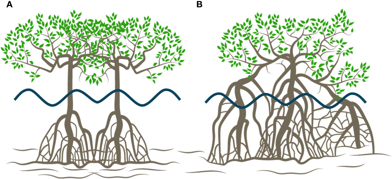
Figure 11 Differences between common three-layer Rhizophora sp. representation (A) in the laboratory and Rhizophora mangle observed in Jicaral, Costa Rica (B).

4.3 Wave attenuation rates

Wave attenuation rates have been used in numerous studies worldwide to evaluate the wave attenuation capacity of distinct mangrove species. When comparing $r$ values, it is important to contrast the particular site conditions between studies (e.g., wave conditions, tidal range, forest characteristics, mangrove species). Supplementary Table 3 present the site characteristics, vegetation species and wave conditions for field studies conducted worldwide (e.g., Mazda et al., 1997a; Brinkman, 2006; Zhou et al., 2022). As can be evidenced, this study present similar wave conditions (Figure 4) to those reported previously with most of the wave conditions not exceeding 20 cm and wave periods ranging between 2 and 6 s. The rates of wave height attenuation obtained along the forest in Jicaral are within the ranges reported by Quartel et al. (2007), with $r$ varying between 0.002 and 0.011 m^-1; Mazda et al. (2006) reported values of approximately 0.0012-0.006 m^-1; and Horstman et al. (2014) reported values of 0.0061 and 0.012 m^-1 for Kantang and Palian, respectively. Studies conducted in the Colombian Caribbean region (Vanegas et al., 2019; Sánchez-Núñez et al., 2020) reported $r$ values higher than those obtained in this study; these values vary between 0.06 and 0.29 m^-1 in a Rhizophora mangle forest, the same species that is present in Jicaral. This difference in $r$ may be attributed to local effects. Vanegas et al. (2019) reported wave attenuation by a mangrove patch of 3.5 m in length in a shallow zone located 1 m from the shore, where dissipation mechanisms, such as breaking and bottom friction, together with the vegetation effect, may lead to high $r$ values. Sánchez-Núñez et al. (2020) reported high slopes at the leading edge of a forest, which produce reflection and wave breaking, influencing $r$. However, the slope measured at the leading edge of the forest in Jicaral was very small, and it did not induce significant wave transformation processes. Despite the variability in $r$ values among studies, these values tend to decrease as water depth increases (Figure 6) and increase as the incident wave height increases (Figure 7), as shown in previous studies (e.g., Mazda et al., 2006; Horstman et al., 2014; Zhou et al., 2022).

4.4 Approaches to obtain ${\tilde{C}}_D$

Several studies have been conducted to obtain ${\tilde{C}}_D$ values in the field; these studies are based on different approaches. Mazda et al. (1997a), Quartel et al. (2007) and Zhou et al. (2022) obtained ${\tilde{C}}_D$ values for different species using the formulation reported by Mazda et al. (1997a), which is based on an equation developed to describe the effect of bottom friction in swell waves under shallow water conditions. The formulation considers the incident and final wave heights, the distance and the mean water depth between both points but does not consider the vegetation characteristics of the studied species. On the other hand, Vanegas et al. (2019) and Sánchez-Núñez et al. (2020) considered vegetation properties by employing the effective vegetation length scale defined by Mazda et al. (1997b), which resulted in high ${\tilde{C}}_D$ values compared to those of other studies (Supplementary Table 3). These ${\tilde{C}}_D$ values were obtained using the methodology presented by Mazda et al. (1997b), which was developed for unidirectional flow conditions and is based on a free surface gradient produced along the forest, which may explain the high coefficients obtained. However, none of these studies reported a predictable formulation for estimating ${\tilde{C}}_D$ by combining hydrodynamics and vegetation properties. In this study, the use of SWAN model allows us to obtain wave energy dissipation produced by vegetation using mangrove trees charactersitics, i.e., the drag force approach (Mendez and Losada, 2004), rather than considering vegetation wave dissipation as an enhancement of bottom friction. Resulting in a predictive formula which has into consideration the inherent spatial vegetation properties and hydrodynamics conditions in the field. Additionally, the calibration was conducted by adjusting the SWAN results against the observed data at multiple locations within the mangrove forest. This approach extends beyond utilizing only two reference points, one offshore and one onshore, as conducted by previous authors. Furthermore, the following approach allows us to obtain ${\tilde{C}}_D$ values associated with only the vegetation effect and by numerically resolving other dissipation processes (such as wave breaking and bottom friction), allowing to quantify their contribution to the total dissipation along the forest (Supplementary Figure 2). In contrast, aforementioned studies, based on field observations and analytical solutions, included all dissipation processes measured in the field when obtaining ${\tilde{C}}_D$ values.

4.5 Canopy influence

The mangrove tree structure in Jicaral mainly consists of roots and trunks, which are difficult to identify, followed by a canopy layer (Figure 3). If the mangrove canopy is not considered, the wave height attenuation may be underestimated when $h$ reaches the canopy height (Maza et al., 2021; Zhang et al., 2023). Based on field observations of the canopy height in the study area, the canopy is expected to influence wave attenuation when the water depth at S1 exceeds 2 m. Based on the cases selected to obtain ${\tilde{C}}_D$(Figure 10), 35% of these cases exceed the water level threshold (black dots in Figure 12), indicating a possible overestimation of ${\tilde{C}}_D$, as the frontal area of the canopy was not characterized nor included in the SWAN model. When the water depth exceeds 2 m, the SWAN model uses a constant frontal area calculated from the geometric tree characteristics measured at a height of 1.5 m above the ground. In this study, cases where the flow reaches the canopy level are still within the scatter (Figure 12). This behavior suggests that when the water depth reaches the canopy level, the interaction between waves and the lower section of the canopy is similar to the interaction between waves and roots. Figure 3 shows that there is no identified interface between roots and the canopy; mixed layers occur at low canopy elevations due to the inherent prostrate growth of Rhizophora mangle, in contrast to the typical three-layer morphology used in several laboratory studies (He et al., 2019; Zhang et al., 2023) and other field campaigns (e.g., Horstman et al., 2014). Therefore, the turbulent structures generated by roots and branches seems to result in similar energy dissipation rates. Nevertheless, further research should be considered to characterize the detailed influence of the canopy on the resultant wave attenuation.

Figure 12

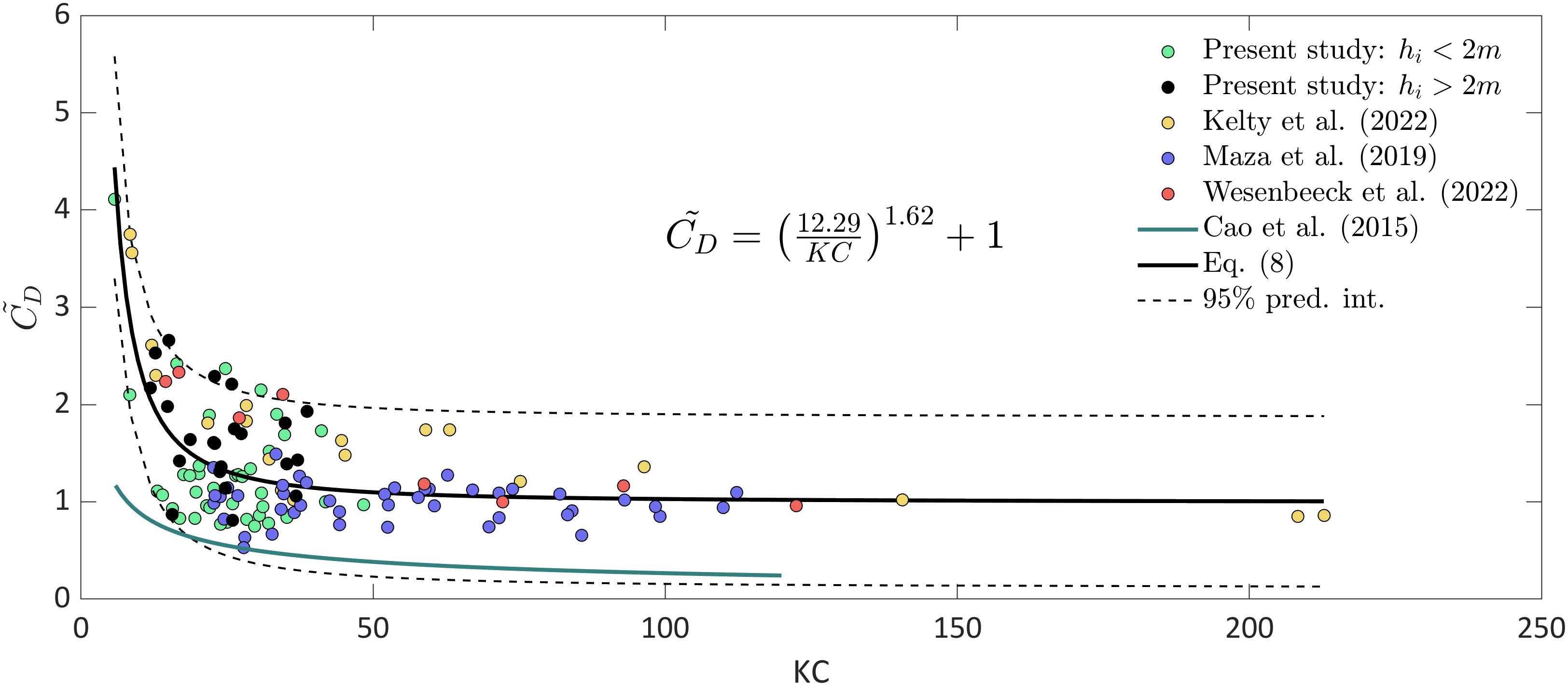
Figure 12 ${\tilde{C}}_D-KC$ relationship for Rhizophora sp. based on field and laboratory data. The cases in the present study are divided into cases where there is an influence of the canopy for incident water depths ($h_i$) greater than 2 m (black dots) and cases where $h_i$< 2 m (green dots).

5 Conclusions

This study presents a new integrated formulation to determine ${\tilde{C}}_D$ as a function of mangrove properties and incident wave conditions, with the purpose to predictably estimate the wave height attenuation produced by Rhizophora forests. The proposed formulation integrates laboratory and field data, defining a characteristic length scale used to estimate ${\tilde{C}}_D$ values. Thus, a field campaign conducted on the Pacific coast of Costa Rica and numerical modeling using the SWAN model are employed to obtain ${\tilde{C}}_D$ values.

The field campaign conducted in Costa Rica, specifically in the Gulf of Nicoya, consisted of 23 days of continuous wave measurements obtained along a Rhizophora mangle forest transect. Additionally, detailed vegetation measurements were collected to characterize the spatial distribution of the forest and its vertical geometric variation. The structure of the sampled vegetation in situ revealed a decrease in root density from the leading edge of the forest toward the inland area. Therefore, the forest frontal area decreases in the direction of wave action. In addition, the Jicaral mangrove forest contains trees with limited structural development, and their prostrate growth impedes clear differentiation between roots and trunks. Hence, the mean root diameter is defined as the characteristic length due to its contribution to the frontal area, which is an obstacle for the waves. Furthermore, in this type of forest, the interface between roots and the canopy is not evident due to its particular structural development, in contrast to the typical Rhizophora three-layer morphology (roots, trunks and canopy) reported in previous studies where there was a clear identification of tree layers. Consequently, these mixed layers make it difficult to identify the influence of the canopy on wave height attenuation with respect to the root layer.

The wave height evolution along the forest is recorded using 5 pressure sensors. On average, the wave height decreased by 34% within 63 m of the forest, which agrees with the values reported in the literature. Additionally, the wave height attenuation rates in Jicaral vary between 0.001 and 0.01 m^-1, which also agrees with the findings of previous field studies conducted in Rhizophora forests. These values are positively correlated with the significant wave height and negatively correlated with water depth.

Currently, empirical formulations for obtaining ${\tilde{C}}_D$ as a function of hydraulic nondimensional parameters for random waves in a Rhizophora sp. forest have been developed based on only laboratory studies without validating their application in the field. To address this gap, ${\tilde{C}}_D$ values are calibrated based on field measurements via numerical modeling. Then, an empirical predictive relationship between ${\tilde{C}}_D$ and $KC$ is developed considering the field data from this study, combined with previous studies conducted in the laboratory. The resulting formulation depends on the correct definition of the root diameter, considered as the characteristic length scale of the trees, and on the orbital velocity associated with the incident wave conditions. Thus, the new formulation allows us to predict ${\tilde{C}}_D$ and can be used in drag force-based approaches to obtain the resulting wave attenuation produced by Rhizophora mangrove forests.

Data availability statement

The original contributions presented in the study are included in the article/Supplementary Material. Further inquiries can be directed to the corresponding author.

Author contributions

FL-A: Conceptualization, Data curation, Formal analysis, Investigation, Methodology, Visualization, Writing – original draft, Writing – review & editing. MM: Conceptualization, Funding acquisition, Methodology, Resources, Supervision, Writing – review & editing. FC: Funding acquisition, Investigation, Resources, Writing – review & editing. GG: Funding acquisition, Resources, Writing – review & editing. JL: Resources, Writing – review & editing.

Funding

The author(s) declare financial support was received for the research, authorship, and/or publication of this article. FL-A was supported by the University of Costa Rica (scholarship OAICE 26-2020). Grant TED2021-130804B-I00 of the project funded by MCIN/AEI/10.13039/501100011033 and by the “European Union NextGenerationEU/PRTR”. Grant PDC2022-133579-I00 of the project funded by MCIN/AEI/10.13039/501100011033 and by the “European Union NextGenerationEU/PRTR”. This study also forms part of the ThinkinAzul programme and was supported by Ministerio de Ciencia e Innovación with funding from European Union NextGeneration EU (PRTR-C17.I1) and by Comunidad de Cantabria.

Acknowledgments

The authors thank Diego Corrales and Ronald Víquez for their work in conducting the topography and bathymetry of the site. Felipe Alfaro, Daniela Quirós and Paula Villegas are also acknowledged for their contribution during the field campaign and Kevin Vargas for his illustration of the mangrove trees.

Conflict of interest

The authors declare that the research was conducted in the absence of any commercial or financial relationships that could be construed as a potential conflict of interest.

Publisher’s note

All claims expressed in this article are solely those of the authors and do not necessarily represent those of their affiliated organizations, or those of the publisher, the editors and the reviewers. Any product that may be evaluated in this article, or claim that may be made by its manufacturer, is not guaranteed or endorsed by the publisher.

Supplementary material

The Supplementary Material for this article can be found online at: https://www.frontiersin.org/articles/10.3389/fmars.2024.1383368/full#supplementary-material

References

Alms V., Romagnoni G., Wolff M. (2022). Exploration of fisheries management policies in the Gulf of Nicoya (Costa Rica) using ecosystem modelling. Ocean Coast. Manag. 230. doi: 10.1016/j.ocecoaman.2022.106349

CrossRef Full Text | Google Scholar

Battjes J. A., Janssen J. P. F. M. (1978). Energy loss and set-up due to breaking of random waves. Coast. Engineer. 569–587. doi: 10.1061/9780872621909

CrossRef Full Text | Google Scholar

Best Ü.S.N., van der Wegen M., Dijkstra J., Reyns J., Van Prooijen B. C., Roelvink D. (2022). Wave attenuation potential, sediment properties and mangrove growth dynamics data over Guyana’s intertidal mudflats: Assessing the potential of mangrove restoration works. Earth Syst. Sci. Data 14, 2445–2462. doi: 10.5194/essd-14-2445-2022

CrossRef Full Text | Google Scholar

Booij N., Ris R. C., Holthuijsen L. H. (1999). A third-generation wave model for coastal regions. J. Geophys. Res. 104, 7649–7666. doi: 10.1029/98JC02622

CrossRef Full Text | Google Scholar

Brinkman R. M. (2006) Wave attenuation in mangrove forests: an investigation through field and theoretical studies. Available online at: http://eprints.jcu.edu.au/1351/.

Google Scholar

Calleja F., Chacón Guzmán J., Alfaro Chavarría H. (2022). Marine aquaculture in the pacific coast of Costa Rica: Identifying the optimum areas for a sustainable development. Ocean Coast. Manag. 219. doi: 10.1016/j.ocecoaman.2022.106033

CrossRef Full Text | Google Scholar

Cao H., Chen Y., Tian Y., Feng W. (2016). Field investigation into wave attenuation in the mangrove environment of the south China sea coast. J. Coast. Res. 32, 1417–1427. doi: 10.2112/JCOASTRES-D-15-00124.1

CrossRef Full Text | Google Scholar

Chang C., Mori N., Tsuruta N., Suzuki K., Yanagisawa H. (2022). An experimental study of mangrove-induced resistance on water waves considering the impacts of typical rhizophora roots. J. Geophys. Res. Oceans 127, 149–154. doi: 10.1029/2022JC018653

CrossRef Full Text | Google Scholar

Dalrymple R. A., Kirby J. T., Hwang P. A. (1984). Wave diffraction due to areas of energy dissipation. J. Waterw. Port Coast. Ocean Eng. 110, 67–79. doi: 10.1061/(ASCE)0733-950X(1984)110:1(67)

CrossRef Full Text | Google Scholar

Duarte C. M., Losada I. J., Hendriks I. E., Mazarrasa I., Marbà N. (2013). The role of coastal plant communities for climate change mitigation and adaptation. Nat. Clim Chang 3, 961–968. doi: 10.1038/nclimate1970

CrossRef Full Text | Google Scholar

Duke N. C., Ball M. C., Ellison J. C. (1998). Factors influencing biodiversity and distributional gradients in mangroves. Global Ecol. Biogeogr. Lett. 7, 27–47. doi: 10.2307/2997695

CrossRef Full Text | Google Scholar

Ewel K. C., Twilley R. R., Ong J. E. (1998). Different kinds of mangrove forests provide different goods and services. Global Ecol. Biogeogr. Lett. 7, 83–94. doi: 10.2307/2997700

CrossRef Full Text | Google Scholar

Gijsman R., Horstman E. M., van der Wal D., Friess D. A., Swales A., Wijnberg K. M. (2021). Nature-based engineering: A review on reducing coastal flood risk with mangroves. Front. Mar. Sci. 8. doi: 10.3389/fmars.2021.702412

CrossRef Full Text | Google Scholar

He F., Chen J., Jiang C. (2019). Surface wave attenuation by vegetation with the stem, root and canopy. Coast. Eng. 152. doi: 10.1016/j.coastaleng.2019.103509

CrossRef Full Text | Google Scholar

Hernández-Blanco M., Costanza R., Cifuentes-Jara M. (2021). Economic valuation of the ecosystem services provided by the mangroves of the Gulf of Nicoya using a hybrid methodology. Ecosyst. Serv. 49. doi: 10.1016/j.ecoser.2021.101258

CrossRef Full Text | Google Scholar

Horstman E. M., Dohmen-Janssen C. M., Narra P. M. F., van den Berg N. J. F., Siemerink M., Hulscher S. J. M. H. (2014). Wave attenuation in mangroves: A quantitative approach to field observations. Coast. Eng. 94, 47–62. doi: 10.1016/j.coastaleng.2014.08.005

CrossRef Full Text | Google Scholar

Hu Z., Lian S., Wei H., Li Y., Stive M., Suzuki T. (2021). Laboratory data on wave propagation through vegetation with following and opposing currents. Earth Syst. Sci. Data 13, 4987–4999. doi: 10.5194/essd-13-4987-2021

CrossRef Full Text | Google Scholar

Jiménez J. (1999). “Ambiente, distribución y características estructurales en los Manglares del Pacífico de Centro américa: Contrastes climáticos,” in Ecosistemas de Manglar en América Tropical. Eds. Yañez-Arancibia A., Lara-Domínguez A. L. (Instituto de Ecología, A.C, Xalapa, México), 51–70.

Google Scholar

Jiménez J., Soto R. (1985). Patrones regionales en la estructura y composición florística de los manglares de la Costa Pacífica de Costa Rica. Rev. Biol. Trop. 33, 25–37.

Google Scholar

Kalloe S. A., Hofland B., Antolínez J. A. A., van Wesenbeeck B. K. (2022). Quantifying frontal-surface area of woody vegetation: A crucial parameter for wave attenuation. Front. Mar. Sci. 9. doi: 10.3389/fmars.2022.820846

PubMed Abstract | CrossRef Full Text | Google Scholar

Kelty K., Tomiczek T., Cox D. T., LoMonaco P., Mitchell W. (2022). Prototype-scale physical model of wave attenuation through a mangrove forest of moderate cross-shore thickness: liDAR-based characterization and reynolds scaling for engineering with nature. Front. Mar. Sci. 8. doi: 10.3389/fmars.2021.780946

CrossRef Full Text | Google Scholar

Koch E. W., Barbier E. B., Silliman B. R., Reed D. J., Perillo G. M. E., Hacker S. D., et al. (2009). Non-linearity in ecosystem services: Temporal and spatial variability in coastal protection. Front. Ecol. Environ. 7, 29–37. doi: 10.1890/080126

CrossRef Full Text | Google Scholar

Lizano O. G. (2007). Climatología del viento y oleaje frente a las costas de Costa Rica. Ciencia y Tecnol. 25, 43–56.

Google Scholar

Loría-Naranjo M., Samper-Villarreal J., Cortés J. (2014). Structural complexity and species composition of Potrero Grande and Santa Elena mangrove forests in Santa Rosa National Park, North Pacific of Costa Rica. Rev. Biol. Trop. 62, 33–41. doi: 10.15517/rbt.v62i4.20030

PubMed Abstract | CrossRef Full Text | Google Scholar

Lugo A. E., Tierra D., Rico P., Snedaker S. C. (1974) The Ecology of Mangroves. Available online at: www.annualreviews.org. doi: 10.1146/annurev.es.05.110174.000351

CrossRef Full Text | Google Scholar

Maza M., Adler K., Ramos D., Garcia A. M., Nepf H. (2017). Velocity and drag evolution from the leading edge of a model mangrove forest. J. Geophys. Res. Oceans 122, 9144–9159. doi: 10.1002/2017JC012945

CrossRef Full Text | Google Scholar

Maza M., Lara J. L., Losada I. J. (2019). Experimental analysis of wave attenuation and drag forces in a realistic fringe Rhizophora mangrove forest. Adv. Water Resour. 131. doi: 10.1016/j.advwatres.2019.07.006

CrossRef Full Text | Google Scholar

Maza M., Lara J. L., Losada I. J. (2021). Predicting the evolution of coastal protection service with mangrove forest age. Coast. Eng. 168. doi: 10.1016/j.coastaleng.2021.103922

CrossRef Full Text | Google Scholar

Mazda Y., Magi M., Ikeda Y., Kurokawa T., Asano T. (2006). Wave reduction in a mangrove forest dominated by Sonneratia sp. Wetl Ecol. Manag. 14, 365–378. doi: 10.1007/s11273-005-5388-0

CrossRef Full Text | Google Scholar

Mazda Y., Magi M., Kogo, Motohiko, Hong P. (1997a). Mangroves as a coastal protection from waves in the Tong King delta, Vietnam. Mangroves Salt Marshes 1, 127–135. doi: 10.1023/A:1009928003700

CrossRef Full Text | Google Scholar

Mazda Y., Wolanski E., King B., Sase A., Ohtsuka D., Magi M. (1997b). Drag force due to vegetation in mangrove swamps. Mangroves and Salt Marshes 1, 193–199. doi: 10.1023/A:1009949411068

CrossRef Full Text | Google Scholar

McIvor A., Möller I., Spencer T., Spalding M. (2012) Reduction of Wind and Swell Waves by Mangroves Natural Coastal Protection Series: Report 1. Available online at: http://www.naturalcoastalprotection.org/documents/reduction-of-wind-and-swell-waves-.

Google Scholar

Mendez F. J., Losada I. J. (2004). An empirical model to estimate the propagation of random breaking and nonbreaking waves over vegetation fields. Coast. Eng. 51, 103–118. doi: 10.1016/j.coastaleng.2003.11.003

CrossRef Full Text | Google Scholar

Menéndez P., Losada I. J., Beck M. W., Torres-Ortega S., Espejo A., Narayan S., et al. (2018). Valuing the protection services of mangroves at national scale: The Philippines. Ecosyst. Serv. 34, 24–36. doi: 10.1016/j.ecoser.2018.09.005

CrossRef Full Text | Google Scholar

Mitsch W. J., Bernal B., Hernandez M. E. (2015). Ecosystem services of wetlands. Int. J. Biodivers. Sci. Ecosyst. Serv. Manag. 11, 1–4. doi: 10.1080/21513732.2015.1006250

CrossRef Full Text | Google Scholar

Norris B. K., Mullarney J. C., Bryan K. R., Henderson S. M. (2017). The effect of pneumatophore density on turbulence: A field study in a Sonneratia-dominated mangrove forest, Vietnam. Cont Shelf Res. 147, 114–127. doi: 10.1016/j.csr.2017.06.002

CrossRef Full Text | Google Scholar

Ohira W., Honda K., Nagai M., Ratanasuwan A. (2013). Mangrove stilt root morphology modeling for estimating hydraulic drag in tsunami inundation simulation. Trees - Structure Funct. 27, 141–148. doi: 10.1007/s00468-012-0782-8

CrossRef Full Text | Google Scholar

Ozeren Y., Wren D. G., Wu W. (2014). Experimental investigation of wave attenuation through model and live vegetation. J. Waterw. Port Coast. Ocean Eng. 140, 04014019. doi: 10.1061/(ASCE)WW.1943-5460.0000251

CrossRef Full Text | Google Scholar

Quartel S., Kroon A., Augustinus P. G. E. F., Van Santen P., Tri N. H. (2007). Wave attenuation in coastal mangroves in the Red River Delta, Vietnam. J. Asian Earth Sci. 29, 576–584. doi: 10.1016/j.jseaes.2006.05.008

CrossRef Full Text | Google Scholar

Sánchez-Núñez D. A., Mancera Pineda J. E., Osorio A. F. (2020). From local-to global-scale control factors of wave attenuation in mangrove environments and the role of indirect mangrove wave attenuation. Estuar. Coast. Shelf Sci. 245. doi: 10.1016/j.ecss.2020.106926

CrossRef Full Text | Google Scholar

Sibaja-Cordero J. A., Gómez-Ramírez E. H. (2022). Marine litter on sandy beaches with different human uses and waste management along the Gulf of Nicoya, Costa Rica. Mar. pollut. Bull. 175. doi: 10.1016/j.marpolbul.2022.113392

CrossRef Full Text | Google Scholar

SINAC (2019). Estrategia regional para el manejo y conservación de los manglares en el Golfo de Nicoya-Costa Rica-2019-2030 (San José, Costa Rica: Programa Nacional de Humedales-Sistema Nacional de Áreas de Conservación).

Google Scholar

Suzuki T., Zijlema M., Burger B., Meijer M. C., Narayan S. (2012). Wave dissipation by vegetation with layer schematization in SWAN. Coast. Eng. 59, 64–71. doi: 10.1016/j.coastaleng.2011.07.006

CrossRef Full Text | Google Scholar

Temmerman S., Horstman E. M., Krauss K. W., Mullarney J. C., Pelckmans I., Schoutens K. (2022). Marshes and mangroves as nature-based coastal storm buffers. Ann. Rev. Mar. Sci. doi: 10.1146/annurev-marine-040422

PubMed Abstract | CrossRef Full Text | Google Scholar

Van Der Lee W. T. B. (1998). “The impact of fluid shear and the suspended sediment concentration on the mud floc size variation in the Dollard estuary, The Netherlands,” in Sedimentary Processes in the Intertidal Zone. Eds. Black K. S., Paterson D. M., Cramp A. (Geological Society, Special Publication, London), 187–198. Available at: http://sp.lyellcollection.org/. doi: 10.1144/GSL.SP.1998.139.01.15

CrossRef Full Text | Google Scholar

Vanegas C. A., Osorio A. F., Urrego L. E. (2019). Wave dissipation across a Rhizophora mangrove patch on a Colombian Caribbean Island: An experimental approach. Ecol. Eng. 130, 271–281. doi: 10.1016/j.ecoleng.2017.07.014

CrossRef Full Text | Google Scholar

van Hespen R., Hu Z., Borsje B., De Dominicis M., Friess D. A., Jevrejeva S., et al. (2023). Mangrove forests as a nature-based solution for coastal flood protection: Biophysical and ecological considerations. Water Sci. Eng. 16, 1–13. doi: 10.1016/j.wse.2022.10.004

CrossRef Full Text | Google Scholar

van Wesenbeeck B. K., Wolters G., Antolínez J. A. A., Kalloe S. A., Hofland B., de Boer W. P., et al. (2022). Wave attenuation through forests under extreme conditions. Sci. Rep. 12. doi: 10.1038/s41598-022-05753-3

CrossRef Full Text | Google Scholar

Vargas J. A. (2016). “The Gulf of Nicoya Estuarine Ecosystem,” in Costa Rican Ecosystems. Ed. Kappelle M. (University of Chicago Press, Chicago), 139–161. doi: 10.7208/chicago/9780226121642.003.0006

CrossRef Full Text | Google Scholar

Wang Y., Yin Z., Liu Y. (2022). Experimental investigation of wave attenuation and bulk drag coefficient in mangrove forest with complex root morphology. Appl. Ocean Res. 118. doi: 10.1016/j.apor.2021.102974

CrossRef Full Text | Google Scholar

Willmott C. J., Robeson S. M., Matsuura K. (2012). A refined index of model performance. Int. J. Climatology 32, 2088–2094. doi: 10.1002/joc.2419

CrossRef Full Text | Google Scholar

Yin Z., Wang Y., Liu Y., Zou W. (2020). Wave attenuation by rigid emergent vegetation under combined wave and current flows. Ocean Eng. 213. doi: 10.1016/j.oceaneng.2020.107632

CrossRef Full Text | Google Scholar

Yoshikai M., Nakamura T., Suwa R., Argamosa R., Okamoto T., Rollon R., et al. (2021). Scaling relations and substrate conditions controlling the complexity of Rhizophora prop root system. Estuar. Coast. Shelf Sci. 248. doi: 10.1016/j.ecss.2020.107014

CrossRef Full Text | Google Scholar

Zhang R., Chen Y., Lei J., Zhou X., Yao P., Stive M. J. F. (2023). Experimental investigation of wave attenuation by mangrove forests with submerged canopies. Coast. Eng. 186. doi: 10.1016/j.coastaleng.2023.104403

CrossRef Full Text | Google Scholar

Zhou X., Dai Z., Pang W., Wang J., Long C. (2022). Wave attenuation over mangroves in the nanliu delta, China. Front. Mar. Sci. 9. doi: 10.3389/fmars.2022.874818

PubMed Abstract | CrossRef Full Text | Google Scholar