Future changes in environmental stressors for the seamount chains of the Southeast Pacific

The submarine seamount chains of Nazca and Salas & Gómez in the Southeast Pacific are areas of high levels of both biodiversity and endemism. The intersection of both ridges is strongly influenced by the Eastern Boundary Upwelling System of the Southeast Pacific and its associated oxygen minimum zone (OMZ). The isolation of individual seamounts and their fragile ecosystems make them extremely vulnerable to any changes in physical and biogeochemical conditions. Here we assess how a number of key physical and biogeochemical variables are projected to change in two climate scenarios using a statistical approach known as quantile regression. This allows the assessment of trends in medians as well as ranges and extremes. Trends in medians show consistent patterns of temperature increase and pH decrease over the entire range of the seamount chains (and entire Southeast Pacific region). Chlorophyll-a appears to show an increase over the majority of the range of the seamounts except at the coast where it decreases. However, the individual seamount chains show contrasting changes for other variables, with the Nazca ridge showing increased oxygen alongside decreasing nutrient levels indicative of decreased upwelling despite contrasting changes in wind stress curl and stratification. Conversely, the Salas & Gómez ridge is projected to see a reduction in oxygen and increased nutrient levels. Alongside these broader patterns in medians, the trends in ranges and extremes are highly variable spatially and less consistent between variables and scenarios. These contrasting changes will provide both advantages and disadvantages depending on the specific species and location of the seamount of interest. These changes present the importance of classifying the desired ranges of the species within these seamount chains and the potentially complex nature of the conservation of these unique but isolated ecosystems.

1 Introduction

In the Southeast Pacific (SEP) lie two submarine seamount chains known as Nazca and Salas & Gómez that run from the coast of Peru southwestwards before ultimately arriving at Rapa Nui (Easter Island), extending a total distance of ~3000 km (Rodrigo et al., 2014). These seamount chains are of particular importance due to the high levels of endemism of the associated biota and the presence of ecologically important species (Wagner et al., 2021; Gaymer et al., 2025). They also support a broader array of animals throughout the region through the habitats they provide and are thus of high conservation value (Friedlander et al., 2021). The intersection of the Nazca and Salas & Gómez ridges is a zone proposed as a biogeographical transition (Parin et al., 1997; Mecho et al., 2021) where two contrasting oceanographic fronts converge: to the east, the Humboldt Current System (HCS), and to the west, oligotrophic subtropical waters (Dewitte et al., 2021). Due to the highly specific nature of the endemic species and the relative isolation of individual seamounts, alongside restricted and small populations, they are particularly vulnerable to any changes in physical and biogeochemical conditions (Clark et al., 2010; Gaymer et al., 2025).

Ocean physics in the SEP is dominated by the South Pacific Anticyclone (SPA), which drives the trade winds that, in turn, induce the upwelling within this eastern boundary upwelling system. This upwelling of colder nutrient rich waters supports the high levels of productivity in the region, making the SEP one of the most productive eastern boundary upwelling systems in the world (Messié and Chavez, 2015). The region has already shown some changes regarding the specific location of the SPA (Weidberg et al., 2020; Aguirre et al., 2021). Projections show this southward shift in the mean location of the SPA is expected to continue (Dewitte et al., 2021). This is associated with projected shifts in mean circulation patterns, which could potentially impact the spatial distributions of key environmental parameters. The impacts of these potential environmental variable changes have already been explored in one study using one CMIP5 model, where the changing metabolic patterns associated with temperature and oxygen were assessed, showing primarily oxygen-based constraints (Parouffe et al., 2023). A broader range of key biogeochemical variables have yet to be fully explored, especially in the latest CMIP6 models.

Changes in the biogeochemistry of the area under a climate change scenario could have enormous impacts on marine biodiversity in general, from primary producers to top predators, both in the benthos and the pelagos. This can impact species distributions and abundances, as recently shown by Gaymer et al. (2024) for several benthic and pelagic species that have crucial ecological, economic and cultural roles in Rapa Nui. Changes of ecologically important species can severely affect marine ecosystems as we know them today with the potential for significant ecosystem restructuring, including by the replacement of niche species, or by ecosystem collapse (e.g., Hare and Mantua, 2000; Wernberg, 2021).

Understanding how ranges are changing over time is crucial to assessing the impact on ecosystems, for example, through the use of species distribution modelling (e.g., Massimino et al., 2017). Studies into the expected ranges of biogeochemical variables have shown potential impacts of climate change, examples include SST, carbon dioxide concentrations, and Chl (Alexander et al., 2018; Landschützer et al., 2018; Zhai et al., 2024). Indeed, changes in variance are expected across all aspects of Earth’s climate, including both physical and biogeochemical variables (Widlansky et al., 2020; Rodgers et al., 2021; Elsworth et al., 2023). In addition, species are expected to be increasingly impacted by extreme events, either by a single stressor or by a combination of multiple (Le Grix et al., 2021; Burger et al., 2022; Hauri et al., 2024). As such, when studying changes, it is crucial to understand how the whole distribution is changing over time.

Due to the importance of monitoring how the distributions of variables of interest are impacted by climate change, we will use a quantile regression technique (Koenker and Bassett, 1978). This provides additional information when compared to the typical approach of linear regression for trend estimation, which could potentially be misleading if parts of the distribution are moving in opposite directions (e.g., Sankarasubramanian and Lall, 2003; Tareghian and Rasmussen, 2013). Quantile regression allows for the estimation of responses at each of a number of specified quantile levels as a proxy for assessing change in the whole distribution of a given variable over time.

This study aims to investigate changes in physical and biogeochemical conditions that may be affecting the seamount chains of the SEP using a number of CMIP6 models climate projections under the SSP245 and SSP585 scenarios. The chosen quantile regression method will allow the assessment of changes in average values as well as their ranges and extremes.

2 Materials and methods

The main focus of this study is on the submarine seamount chains of Nazca and Salas & Gómez, however, a larger domain will be used for the study area to understand the broader region and how effects elsewhere may be impacting the seamount chains, as such the entire domain runs from 50°S to 10°N and extends longitudinally from the coast to 120°W. Data from the surface to 600m depth is considered; this covers the depth range where the majority of the seamount summits are present and represents where the majority of biological and physical observational data will be collected in the future. Variables that were used for consideration cover the primary stressors expected to impact life on the seamounts and include temperature, salinity, O₂ (dissolved oxygen), pH, CO₃ (carbonate), NO₃ (nitrate) and Chl (Chlorophyll-a). Temporally, two periods were used: 1950-2014 (i.e., of the historical scenario), note that 1950 was chosen as the lower limit as this allowed the period to be directly validated with observations; and the period 2014-2100 using climate projections under low and high emissions scenarios (SSP245 and SSP585 respectively). These extended time periods allow for climate change driven trends to be distinguished from natural background variability (Henson et al., 2016), Model data from four separate CMIP6 models and their ensembles were used, see Table 1 for details, all downloaded from the ESGF portal (Eyring et al., 2016). Trends were estimated for each model after averaging across all available ensembles, to avoid giving undue weight to models with more ensembles. The results are presented as multi model averages of the trend on a grid that matches that of the highest resolution in horizontal (CNRM-CM6-1-HR: ~0.25°) and vertical (CESM2: 35 levels between 0 and 600 m, spacing increasing from 5 to ~50 m) space. The models were individually validated against all available observations within the domain taken from the World Ocean Database 18 (Boyer et al., 2018) - see supplementary information.

Table 1

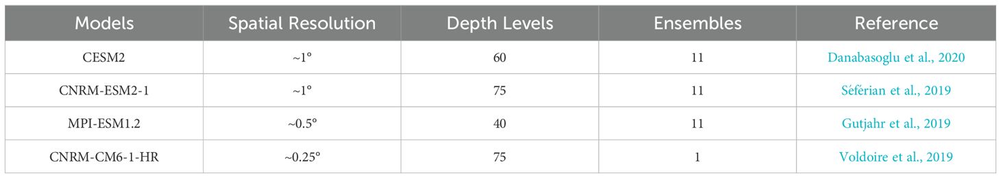
Table 1. List of CMIP6 models used in the study and their key details and references.

In order to estimate change in the distributions of our variables of interest, we use quantile regression (Koenker and Bassett, 1978). Here we choose 5 quantile levels (q) to assess: 5%, 25%, 50%, 75%, and 95%. These range of values allow assessment of trends in the median, inter-quartile range (IQR) (i.e., the difference between the 25% and 75% quantiles, representing the centre 50% of the distribution), and high and low extremes. The quantile regression model we use is expressed as:

$$y_q={\alpha }_q+{\beta }_{q}t$$

where the conditional quantile ($y_q$) varies as a function of the intercept (α_q) and slope (β_q) again both at a given quantile, observations at time (t= 1,2,…,n) (months). The parameters of the regression model for each (q) quantile are estimated by minimising the tiled absolute value function.

Many natural variables can be expected to demonstrate serial autocorrelation in their time series. Such autocorrelation has been previously shown to bias trend detection if not properly accounted for in the cases of both linear (Beaulieu et al., 2013) and quantile (Huo et al., 2017; Koenker, 2017) regression. As such, we first test for autocorrelation, and if it is detected, the time series is then transformed to correct for the autocorrelation, following the methodology employed by Zhai et al. (2024). The approach assumes that residuals in the time series can be represented by a first order autocorrelation (AR(1)) model. To test if autocorrelation is indeed present a QF test, a residual based autocorrelation test, is employed (Huo et al., 2017). If the QF test is positive and serial autocorrelation is shown to be present in the residuals, the time series is then transformed following Cochrane and Orcutt (1949).

3 Results

3.1 Trends for the South East Pacific

First, the spatial patterns of trends in the median were assessed across the whole region at 300 m depth, the half way point of depths analysed, except for Chl which was analysed at the surface (Figure 1). Inter-model uncertainty was also assessed for all trends - see Supplementary Information. A number of variables show trends of the same sign across the whole region, namely temperature showing increases and decreases in both pH and CO₃. Salinity shows a positive trend over the north and east of the region, largely associated with the Humboldt system upwelling region (called hereafter upwelling region), showing a decrease in the rest of the domain. Oxygen shows an overall decreasing trend in the domain except in the core OMZ region in the junction between Chile and Peru, which includes the Nazca ridge, where it shows an increase. Chl shows a decrease at the coast, with an increase over the majority of the rest of the seamount chains, strongest at the edge of the South Pacific Gyre, although no trend is observed in its centre. There is general agreement between the two climate scenarios in all cases.

Figure 1

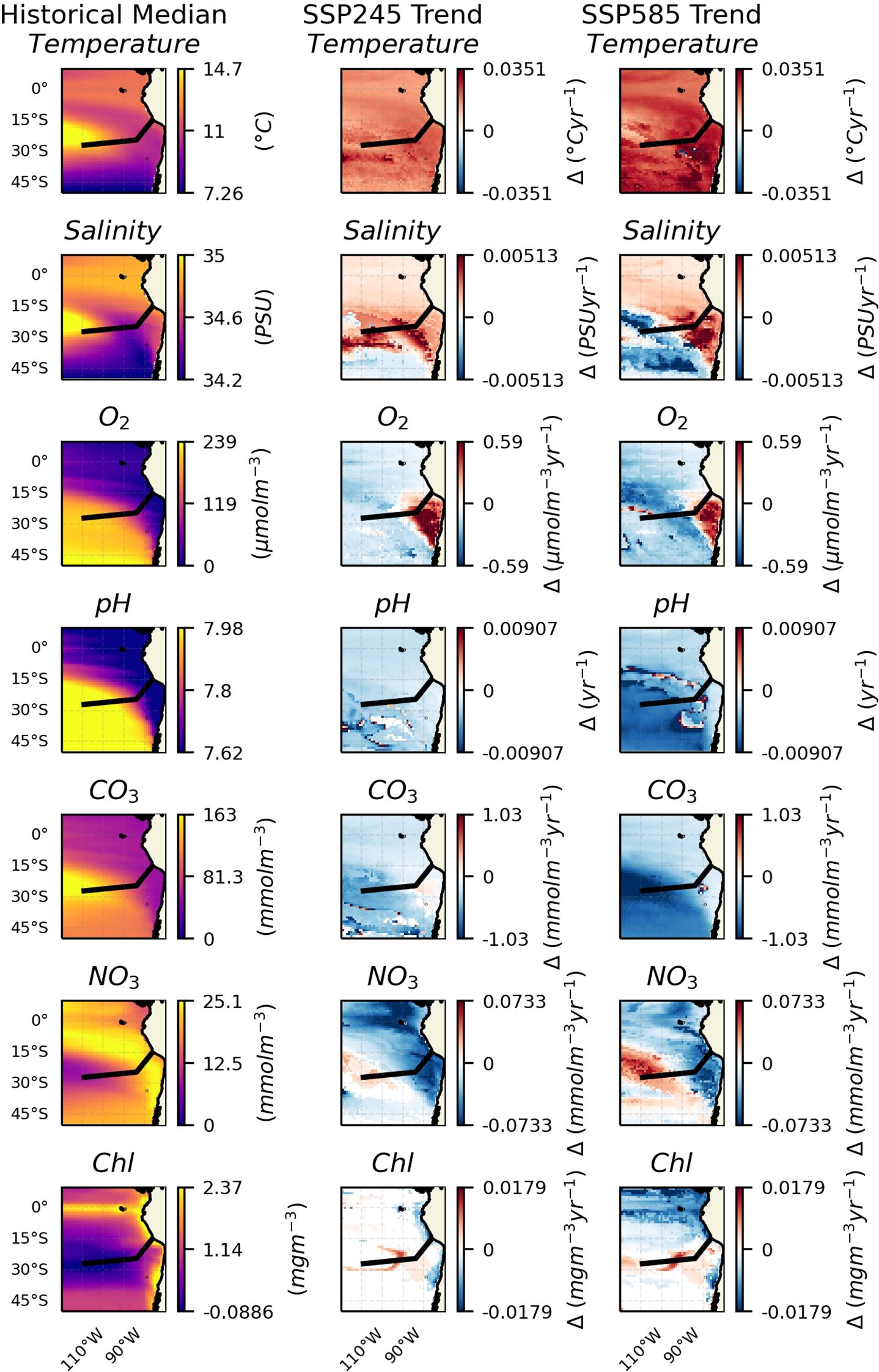
Figure 1. Key variables at 300 m depth across the region. The black line shows the approximate chord along the seamount chains. The leftmost column shows the median values for the historic period. The middle column shows trends in the median over the SSP245 period. And the rightmost shows trends in the median over the SSP585 period. Insignificant trends are considered as 0 (i.e., in white).

Trends in the IQR over the same domain and depth were also assessed (Figure 2). A markedly less consistent pattern between the two climate scenarios and individual variables is seen. Of the spatial patterns in trends that are more consistent: temperature shows an overall positive trend in IQR towards the coast, particularly in the SSP585 scenario. Salinity shows a generally positive trend in the 20°S to 40°S latitude range, the western portion of this appearing to relate to the location of the South Pacific Gyre. Oxygen concentration appears to show a decrease in IQR centred around the transition zone between the two seamount chains, likely associated with the edge of the OMZ. Carbonate concentration appears to show a negative trend in IQR over the Salas & Gómez ridge, although in this case, it is not matched by a similar decrease in the IQR of pH. Nitrate concentration appears to show a trend towards increased IQR over the upwelling region and a decrease in the rest of the domain. Chl seems to show no IQR trend in the SSP245 scenario, and only scattered increases and decreases in the SSP585 scenario.

Figure 2

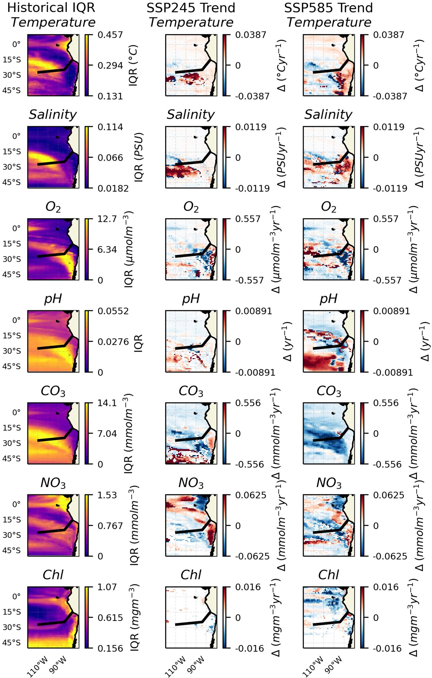
Figure 2. Key variables at depths of 300 m across the region. The black line shows the approximate chord along the seamount chains. The leftmost column shows the IQR values for the historic period. The middle column shows trends in IQR over the SSP245 period. And the rightmost shows trends in IQR over the SSP585 period. Insignificant trends are considered as 0 (i.e., in white).

Finally, trends in the low and high extremes (5% and 95% quantiles) were assessed (Figure 3). Compared to the IQR and median, trends in the extremes show even less consistency between the climate scenarios and individual variables. Of the more consistent patterns, temperature shows an increasing trend in both scenarios at both ends of the distribution, indicative of the whole distribution shifting. Nitrate concentration appears to show a decreasing trend for the 5% quantile over the upwelling region and an increase over the rest of the domain. Chl appears to show a contraction of the extremes (i.e., towards a distribution with reduced tails) with a negative trend in the high extremes and positive trend in the low extremes, particularly centred towards the eastern end of the Salas & Gómez ridge.

Figure 3

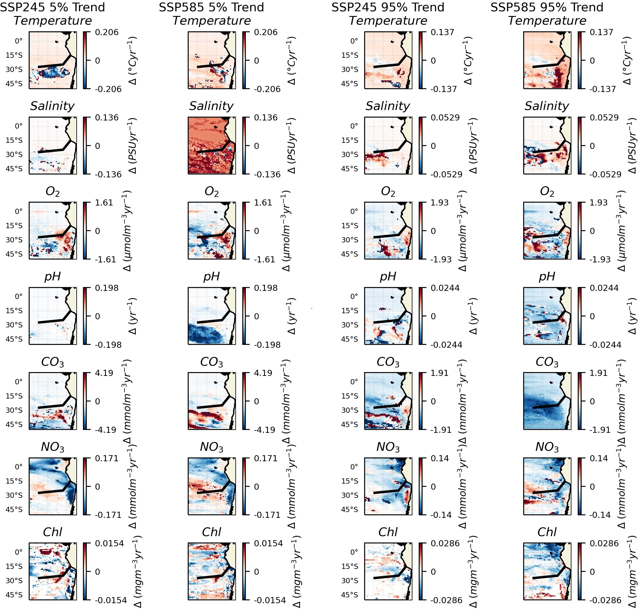
Figure 3. Key variables at depths of 300 m across the region. The black line shows the approximate chord along the seamount chains. The two left columns show changes in the 5% quantile. The two right columns show trends in the 95% quantile. For each pair, the left column shows trends over the SSP245 period and the right column shows changes over the SSP585 period. Insignificant trends are considered as 0 (i.e., in white).

3.2 Trends with depth along the seamount chains

Following the assessment at 300 m depth across the whole region, trends in the median were evaluated along the two seamount chains at depths between 0 and 600 m (Figure 4). Similarly to the regional plots of median trend, temperature shows an increase at all depths, while pH and CO₃ show a decrease across all depths. In general, salinity shows a positive trend in the median, except in a subsurface core towards the centre of the region, which shows a negative trend. Oxygen generally decreases, except in the OMZ where it shows an increase. Nitrate concentration shows a positive trend in the median in areas that had low values in the historical period, i.e.,. towards the surface and West, and a decreasing trend where values were previously highest, i.e., towards the deep and East.

Figure 4

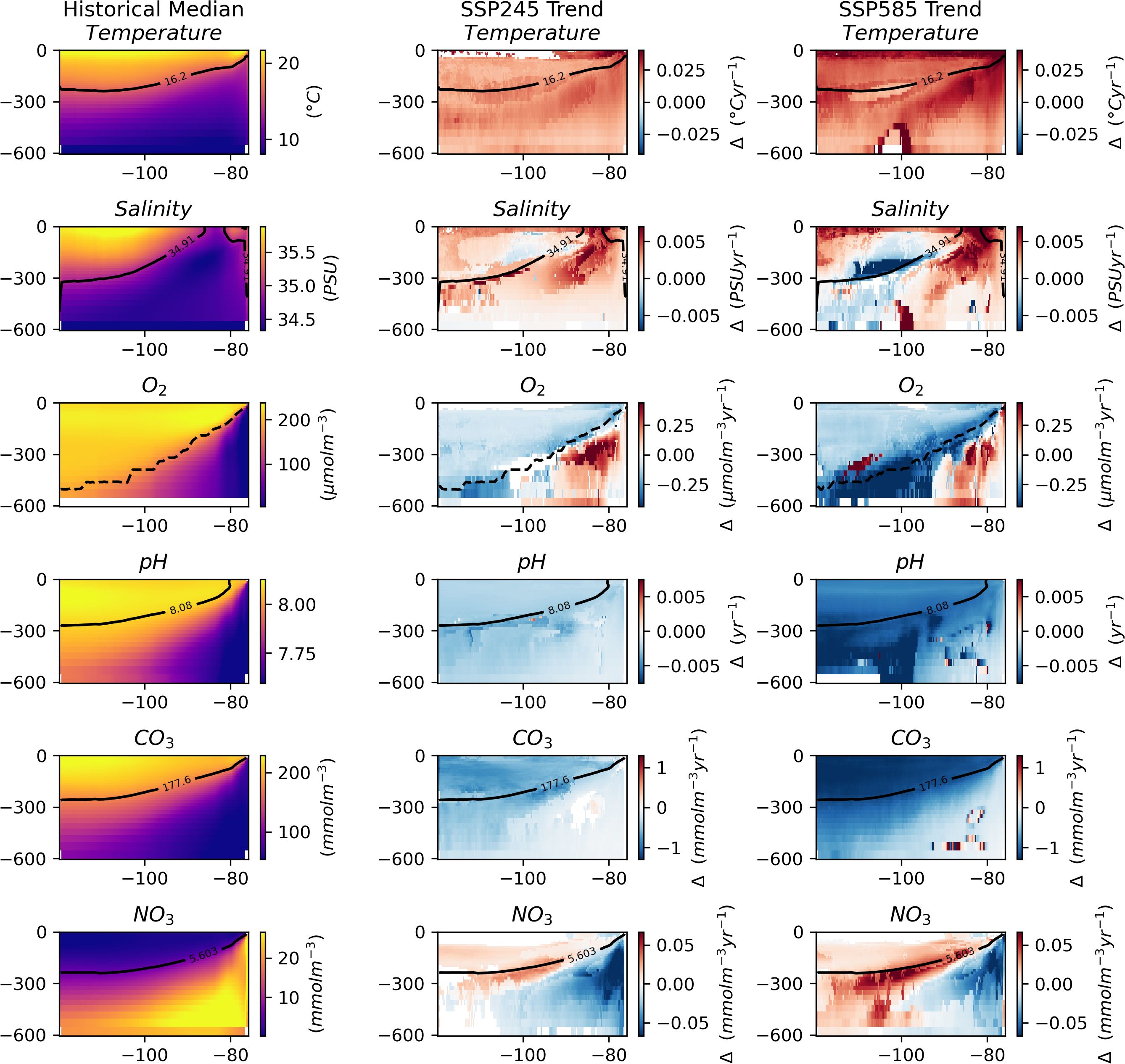
Figure 4. Key variables with depth across the length of the combined seamount chains. The leftmost column shows the median values for the historic period. The middle column shows trends in the median over the SSP245 period. And the rightmost shows trends in the median over the SSP585 period. Insignificant trends are considered as 0 (i.e., in white). The solid black line indicates the depth of the median value in the historical period. The dashed black line indicates the depth of the oxycline.

Similarly to the regional patterns in IQR trends, trends in IQR along the cross-section do not show much of a consistent pattern (Figure 5). The historical IQR subplots reveal an area of increased IQR that extends diagonally from shallow depths in the East to deeper depths in the West. This feature likely reflects the boundary of the upwelling/OMZ, indicating variability in the exact location over time. Notably, trends in the IQR of oxygen concentration show a negative trend in this particular zone, closely matched by an increase towards the West and at slightly shallower depths. pH and nitrate concentrations appear to show a related change, although with less consistency.

Figure 5

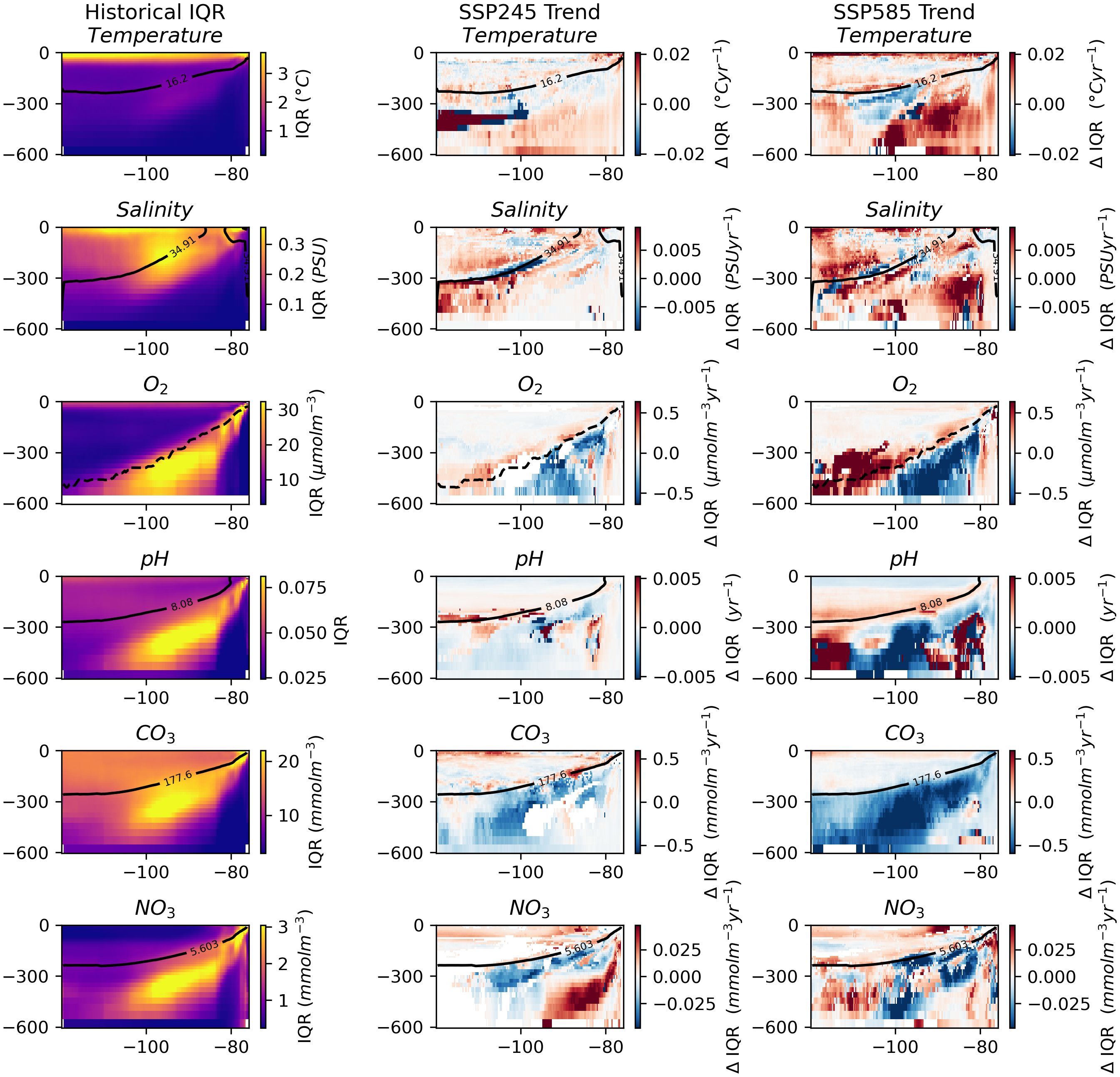
Figure 5. Key variables with depth across the length of the combined seamount chains. The leftmost column shows the IQR values for the historic period. The middle column shows trends in IQR over the SSP245 period. And the rightmost shows trends in IQR over the SSP585 period. Insignificant trends are considered as 0 (i.e., in white). The solid black line indicates the depth of the median value in the historical period. The dashed black line indicates the depth of the oxycline.

Trends in the extreme quantiles (Figure 6) do appear to show more consistency as compared to the regional assessment. For the trends in the extreme quantiles of temperature and salinity, both the 5% and 95% quantiles are increasing over the majority of the cross section, indicating a shift in the whole distribution towards higher values, although note the negative movement in the median of salinity towards the centre of the region in the previous section. Carbonate concentration shows an overall decrease in both extreme quantiles across both scenarios. Oxygen concentration shows a positive trend in the 5% quantile and decrease in the area of historically highest IQR, consistent with the trends in IQR showing a narrowing distribution here. Towards the surface, nitrate concentration shows a negative trend in the 5% quantile and positive trend in the 95% quantile indicative of an increased likelihood of both extremes. At depth towards the East, the nitrate concentration trends in both extremes show an overall decrease, possibly linked to changes in upwelling.

Figure 6

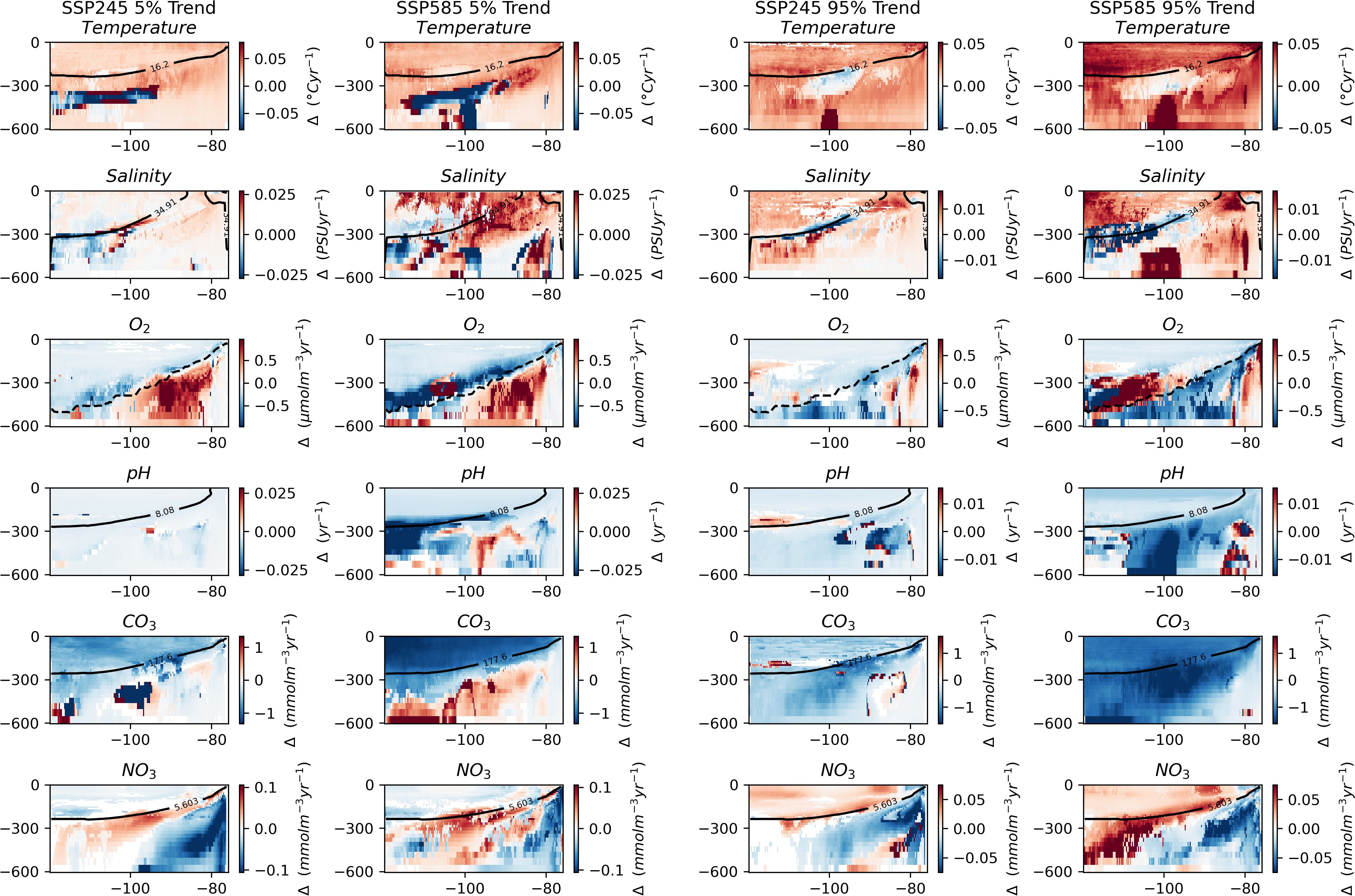
Figure 6. Key variables with depth across the length of the combined seamount chains. The two left columns show changes in the 5% quantile. The two right columns show trends in the 95% quantile. For each pair,the left column shows trends over the SSP245 period and the right column shows changes over the SSP585 period. Insignificant trends are considered as 0 (i.e., in white). The solid black line indicates the depth of the median value in the historical period. The dashed black line indicates the depth of the oxycline.

4 Discussion

This manuscript addresses changes in physical and biogeochemical conditions along the Nazca and Salas & Gómez submarine chains in the SEP, evaluating climate projections from CMIP6 models under the SSP245 and SSP585 scenarios.

The key variables showing spatially constant trends in the median are the temperature increases and pH/carbonate decreases. These are consistent in direction with the findings in Dewitte et al. (2021). pH changes are expected to impact a number of the endemic species in the region, particularly those that precipitate calcium carbonate (Hofmann et al., 2010). Temperature changes would be expected to provide a particular constraint on metabolism, especially outside the OMZ, where oxygen has been shown to be the dominant constraint (Parouffe et al., 2023). Increasing temperature is also generally expected to impact ectotherm phenology, geographic distribution and lead to a reduction in species body size (e.g., Ohlberger, 2013).

The other main pattern of changes relates to the OMZ/upwelling region, where oxygen concentration is projected to increase and nutrient availability decrease. The changes in oxygen are consistent with trends observed in the CESM-LE (Community Earth System Model - Large Ensemble) (Dewitte et al., 2021; Parouffe et al., 2023). We note that there appears to be negligible change in wind speed over the region in the SSP245 scenario, and although there are increases in the SSP585 scenario, they are focused away from the core of the oxygen minimum zone (Figure 7). However, wind stress curl (Figure 8), at least in the SSP585 scenario, shows trends towards increasing Ekman suction over the Nazca seamount chain, indicative of an increase in upwelling. Other research has noted a weak increase in upwelling favourable winds (Chamorro et al., 2021). Conversely, strong surface temperature increases (Figure 4) may be enhancing stratification and which is an opposing control on upwelling. Mixed layer depth (MLD) is predicted to shallow over the extent of the Nazca ridge (Figure 9). Eastern boundary upwelling systems have generally seen an increase in wind-driven upwelling leading to broader (e.g., Frederick et al., 2024) and stronger (e.g., Chan, 2019) OMZs although others have noted this conflict between temperature and wind-driven controls (e.g., Dewitte et al., 2021). These conflicting trends may ultimately lead to a partially compensatory effect of climate change impacts on productivity. Alongside this change in intensity, there appears to be changes in variability along the boundary of the OMZ, as represented by the oxycline, with increased variability at shallower depths and to the west and decreased variability at deeper depths to the east (Figure 5). This change in variability may relate to changes in subsurface mesoscale activity along the border; such dynamics have been shown to have an important role at the border of the Peruvian OMZ (Bettencourt et al., 2015).

Figure 7

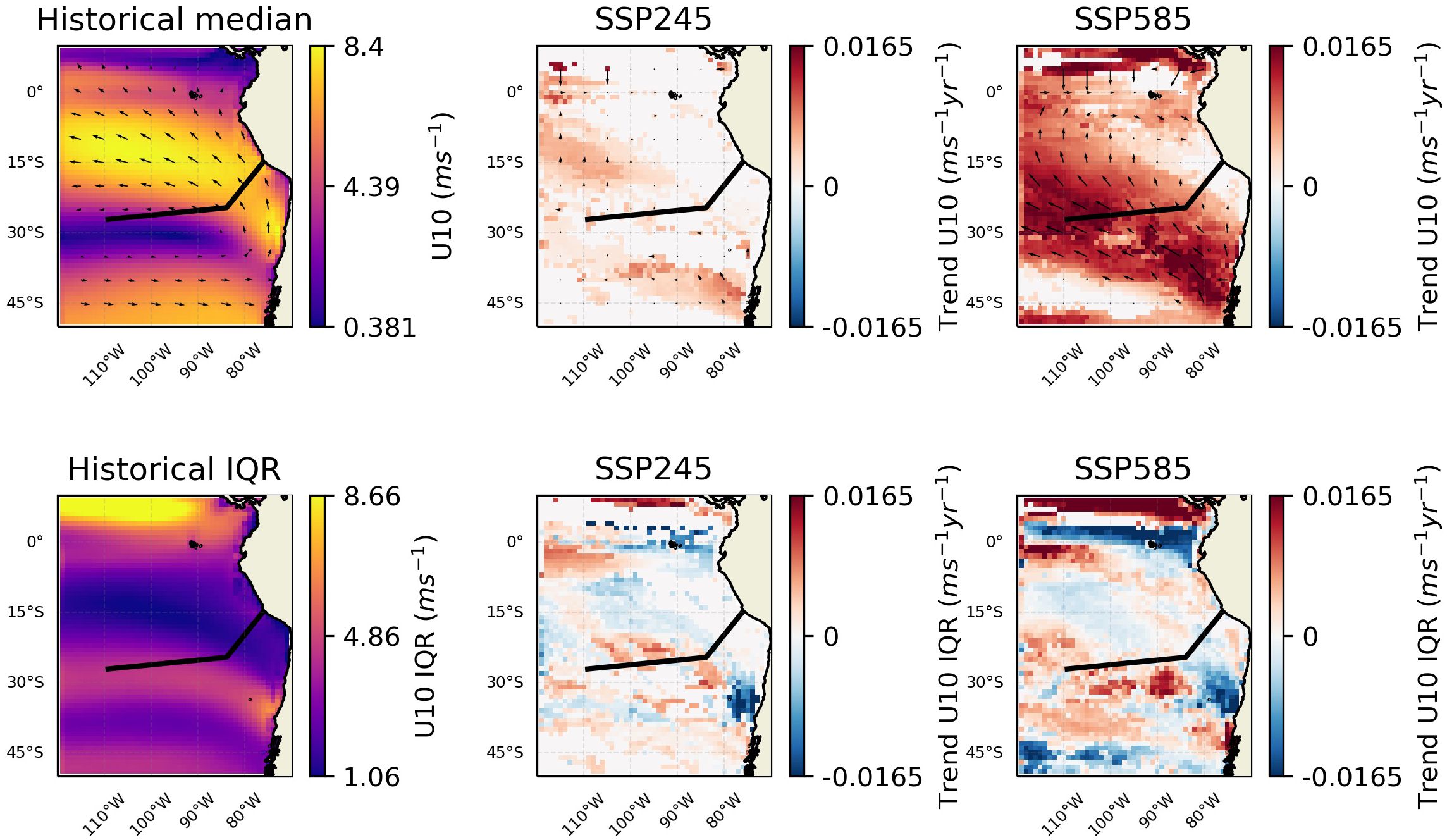
Figure 7. Changes in wind speed and direction over the region. The black line shows the approximate chord along the seamount chains. The leftmost column shows the values for the historic period. The middle column shows trends over the SSP245 period. And the rightmost shows trends over the SSP585 period. The top row shows medians and the bottom row IQR. Insignificant trends are considered as 0 (i.e., in white).

Figure 8

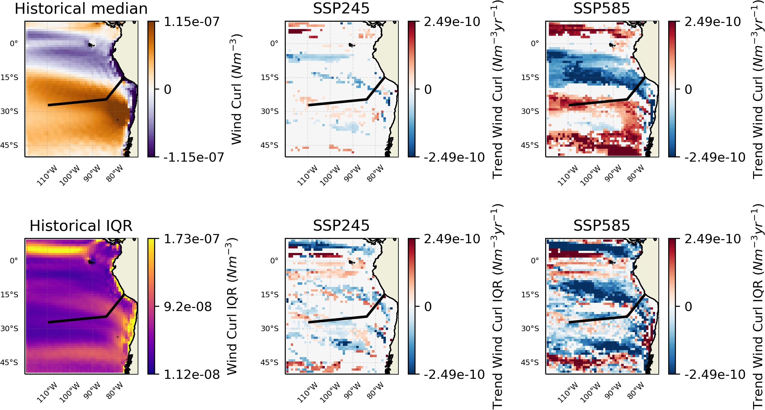
Figure 8. Changes in wind stress curl over the region. The black line shows the approximate chord along the seamount chains. The leftmost column shows the values for the historic period. The middle column trends over the SSP245 period. And the rightmost trends over the SSP585 period. The top row shows medians and the bottom row IQR. Insignificant trends are considered as 0 (i.e., in white).

Figure 9

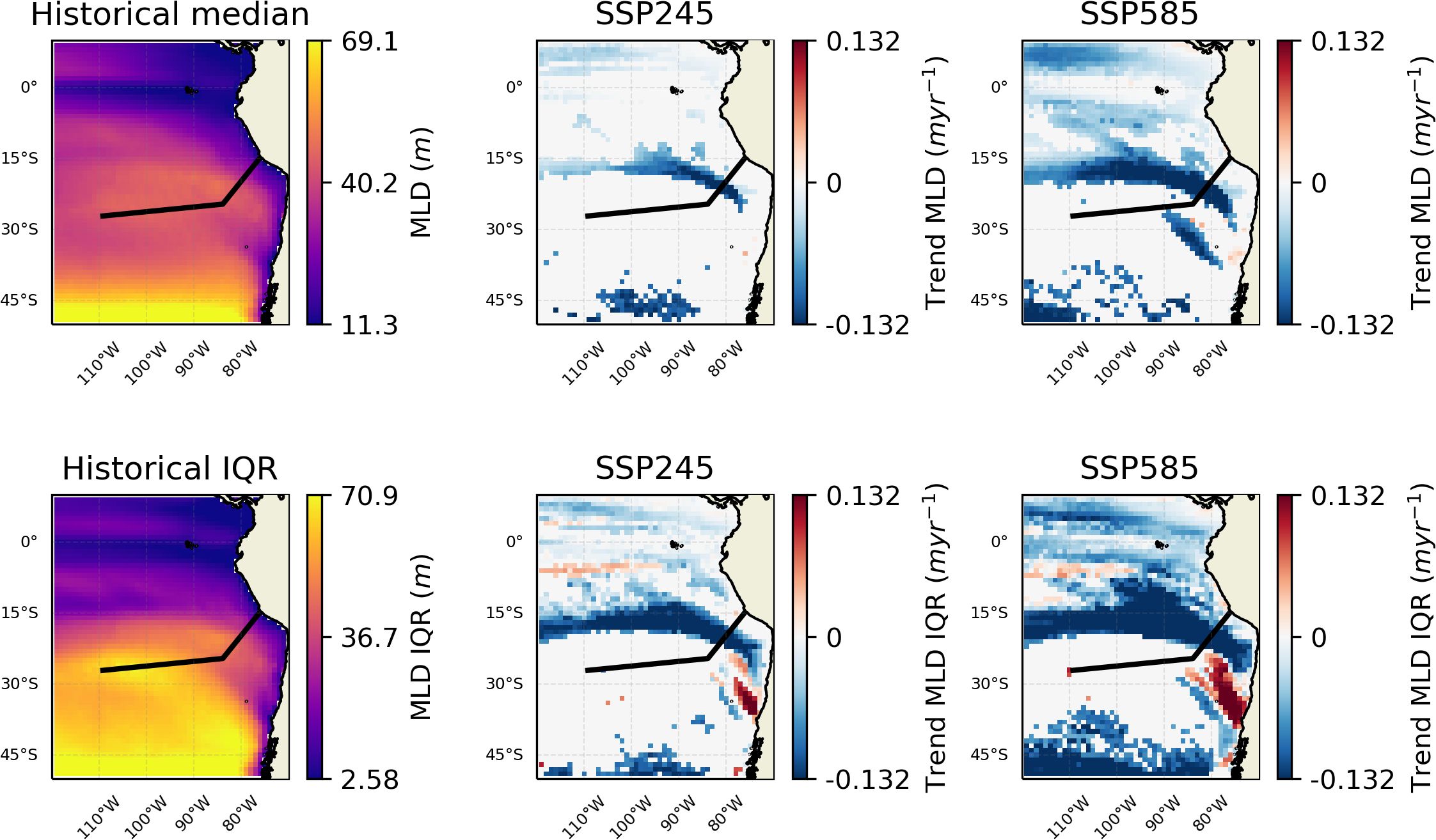
Figure 9. Changes in MLD (Mixed Layer Depth) over the region. The black line shows the approximate chord along the seamount chains. The leftmost column shows the values for the historic period. The middle column trends over the SSP245 period. And the rightmost trends over the SSP585 period. (Blue indicates a shallowing MLD). The top row shows medians and the bottom row IQR. Insignificant trends are considered as 0 (i.e., in white).

These upwelling-related changes appear to lead to contrasting trends between the two seamount chains, as the boundary between them also happens to lie at the edge of the upwelling zone (Figure 10). This means that for the Salas & Gómez chain, where nutrients are already lower due to the presence of the South Pacific Gyre, an increase in nutrient variability and Chl concentrations will be beneficial, although a decrease in oxygen concentrations may start to impose metabolic constraints, even if oxygen concentrations should still be substantially above hypoxia. Conversely, the Nazca chain, where nutrients in the historical period were more abundant, may start to suffer nutrient limitation, while oxygen constraints may be relaxed. Jack mackerel (Trachurus murphyi) have a nursery area in the region of the Nazca seamount chain and have been shown to avoid low oxygen zones (Bertrand et al., 2016), so this may well increase their distribution here. However, the resident fauna of the OMZ of the Nazca Ridge could be affected by modifications in the trophic web or the entry of competing non-resident fauna, through distribution changes.

Figure 10

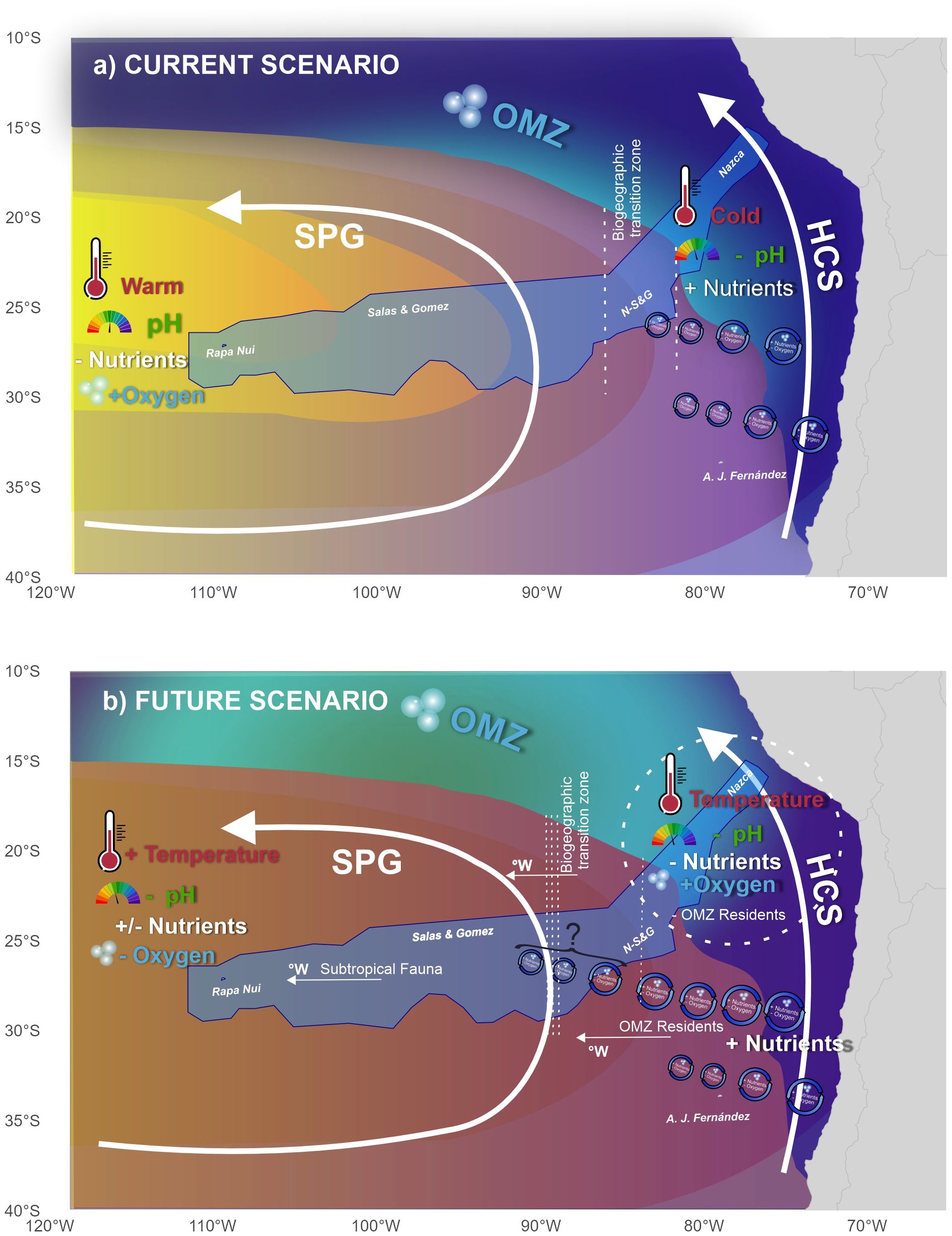
Figure 10. Conceptual model of current conditions and potential future changes and their effect on benthic fauna. The blue polygon represents the EBSA (Ecologically or Biologically Significant Areas) of the Salas & Gómez and Nazca Ridges. OMZ, Oxygen Minimum Zone; HCS, Humboldt Current System; SPG, South Pacific Gyre.

The models show changes in the physical and biochemical conditions at the intersection of the Nazca and Salas & Gómez ridges, a zone proposed as a biogeographical transition (Parin et al., 1997; Mecho et al., 2021), where two contrasting oceanographic fronts converge: to the east, influenced by the HCS, and to the west, by oligotrophic subtropical waters (Dewitte et al., 2021). Along the Salas & Gómez ridge, the intersection is the area with the highest diversity of mesophotic communities. Changes in oxygen, temperature, and nutrient conditions could alter community structure, connectivity patterns, and the bathymetric and longitudinal distribution of both invertebrates and vertebrates (Bertrand et al., 2016). The projected increase in temperature and Chl, and decrease in pH across the entire SEP region, as indicated by our results, will also have significant implications for seabirds. Warmer waters can alter the distribution and abundance of prey species, which is crucial for seabirds’ foraging success. For example, studies by Lerma et al. (2020) and Serratosa et al. (2020) highlight the importance of oceanographic conditions in shaping the foraging ecology and at-sea distribution of seabirds. The increased variability and extremes in physical and biogeochemical variables will expose seabirds to more frequent and severe environmental stressors. This heightened variability can disrupt the stability of seabird populations, as they may struggle to adapt to rapid changes in their environment. Plaza et al. (2021) observed temporal changes in seabird assemblage structure and trait diversity in Rapa Nui, highlighting the sensitivity of seabird communities to environmental fluctuations.

The prediction that nutrients will increase, and dissolved oxygen will decrease westwards and the opposite eastwards, poses an interesting scenario, where the traditionally ultraoligotrophic Salas y Gómez ridge will tend to face conditions more like those present in the Nazca ridge. This means that some species and biogeographic breaks could move westwards and thus conservation measures should consider future changes in biodiversity composition. Due to these types of changes, conservation tools such as mobile protected areas have been suggested for mobile species (Maxwell et al., 2020). Although hard to enforce, mobile protected areas could be useful for highly mobile fishes, sea turtles, seabirds and marine mammals. However, benthic sessile species that dominate both ridges are not able to migrate and will have to either adapt to changes in conditions or extend their distribution ranges. Thus, adaptive management strategies will be needed when planning for conservation measures such as those suggested in Gaymer et al. (2025).

Although changes in the median do appear to show clear patterns in the region that are consistent between the investigated climate scenarios, when trends in the IQR and high and low extremes are investigated less spatially consistent patterns are seen; indeed, changes in ranges and extremes appear likely to affect small portions of the investigated seamount chains, making broader conclusions hard to draw. The origin of this increased variability is likely from an increase in transitory events such as fronts and eddies that are increasing in activity as a result of temperature increases and associated changes in wind and current magnitude and directions. Such changes have been noted to be complex and multi-faceted globally, although changes in this region are projected to be smaller than others (Beech et al., 2022). Frontal probability has been noted to be increasing in sub-regions of the SEP (e.g., Oerder et al., 2018). Note that the available resolution of the CMIP6 models used may impact the size and location of these individual sub-regions as a response to the smaller scale meso and submesoscale events which are likely underrepresented here.

The CMIP6 models used here are of relatively coarse resolution compared (¼ ° - 1°) to regional models (typically ≤ 1/10°) meaning that mesoscale and submesoscale features, including eddies, vortices, fronts, and filaments, are likely not to be represented properly despite being an important source of variability. This may be of particular importance along the edge of the OMZ and with dynamics around the individual seamounts themselves, i.e., similar to the island mass effect; their topography has been shown to affect circulation patterns and enhance vertical mixing (Vic et al., 2019) locally increasing nutrient concentrations (Rowden et al., 2020). These finer scale dynamics would likely lead to increased variability than is seen here, and may also change average patterns. Likewise, eddies are seen as a possible source of deoxygenation and nutrient supply away from the coastal zone towards the deeper ocean (D’Ottone et al., 2016). Unfortunately, at this stage, CMIP6 models with sufficient biogeochemical variables are limited; regional models of higher resolution that include climate projections should be explored to understand potential changes and impacts in these features on biogeochemistry and, thus, ecology.

5 Conclusions

This study focused on assessing trends in climate projections for a number of key variables, both physical and biogeochemical in the seamount chains of Nazca and Salas & Gómez in the Southeast Pacific. We used output from a number of CMIP6 models over both low (SSP245) and high (SSP585) emission scenarios and analysed these using a quantile regression approach to understand changes in average, ranges, and extremes.

Our findings indicate that for the entire region at depths to 600 m, temperature is projected to increase in both scenarios associated with a corresponding increase in acidity (i.e., decrease in pH). Alongside these overall changes for the entire domain, the contrast between the coastal upwelling system, covering the Nazca ridge and an open ocean regime, covering the Salas & Gómez ridge are seen. These show an increase in nutrients and a decrease in oxygen over the Salas & Gómez ridge and the opposite over the Nazca ridge (Figure 10). These trends appear to be linked to changes in upwelling strength through the competing impacts of enhanced temperature-driven stratification and wind stress curl. Chl does not appear to show trends closely tied to that of nutrients or wind showing an increase along the ridges except at the coast where it decreases. Changes in IQR and extremes show increased spatial variability and lower coherency over the entire region when compared to the median, although patterns are indicative of changing variability along the boundary of the OMZ. Overall, these results show significant changes, smaller than the inter-model uncertainty, for these seamount chains and the entire South East Pacific, although the complex nature of changes in the trends in ranges challenges the development of an overall conservation approach.

Future work should focus on assessing how these changes in physical and biogeochemical variables will impact these organisms by using the trends here as input for changes in a species distribution modelling approach. Following this, application of regional modelling for assessing climate projections can be used to understand the different impacts on the variability and average state from broader-scale to mesoscale and submesoscale features such as fronts and eddies.

Data availability statement

Publicly available datasets were analyzed in this study. This data can be found here: https://esgf.llnl.gov/ https://www.ncei.noaa.gov/products/world-ocean-database.

Author contributions

MH: Conceptualization, Formal analysis, Investigation, Methodology, Software, Visualization, Writing – original draft, Writing – review & editing. MR: Methodology, Project administration, Supervision, Writing – original draft, Writing – review & editing. MG: Visualization, Writing – review & editing. DZ: Methodology, Software, Writing – review & editing. EF: Writing – review & editing. CG: Funding acquisition, Project administration, Supervision, Writing – review & editing. JS: Funding acquisition, Project administration, Supervision, Writing – review & editing. GL-J: Funding acquisition, Project administration, Supervision, Writing – review & editing.

Funding

The author(s) declare that financial support was received for the research and/or publication of this article. This work was funded by Anillo BiodUCCT (ATE 220044). This research was also supported by the Center for Ecology and Sustainable Management of Oceanic Islands (ESMOI). MLH received support from Concurso de Fortalecimiento al Desarrollo Científico de Centros Regionales 2020-R20F0008-CEAZA.

Acknowledgments

We would like to thank the World Climate Research Programme, which, through its Working Group on Coupled Modelling, coordinated and promoted CMIP6. We also wish to thank the individual climate modeling groups for producing and making available their model output, the Earth System Grid Federation (ESGF) for archiving the data and providing access, and the multiple funding agencies who support CMIP6 and ESGF. We would also like to thank the team behind the World Ocean Database for making their product available.

Conflict of interest

The authors declare that the research was conducted in the absence of any commercial or financial relationships that could be construed as a potential conflict of interest.

Generative AI statement

The author(s) declare that no Generative AI was used in the creation of this manuscript.

Publisher’s note

All claims expressed in this article are solely those of the authors and do not necessarily represent those of their affiliated organizations, or those of the publisher, the editors and the reviewers. Any product that may be evaluated in this article, or claim that may be made by its manufacturer, is not guaranteed or endorsed by the publisher.

Supplementary material

The Supplementary Material for this article can be found online at: https://www.frontiersin.org/articles/10.3389/fmars.2025.1550708/full#supplementary-material

References

Aguirre C., Garreaud R., Belmar L., Farías L. (2021). High-frequency variability of the surface ocean properties off central Chile during the upwelling season. Front. Marine Sci. 8. doi: 10.3389/fmars.2021.702051

Crossref Full Text | Google Scholar

Alexander M. A., Scott J. D., Friedland K. D., Mills K. E., Nye J. A., Pershing A. J., et al. (2018). Projected sea surface temperatures over the 21st century: changes in the mean, variability and extremes for large marine ecosystem regions of northern oceans. Elementa 6, 73–84. doi: 10.1525/elementa.191

Crossref Full Text | Google Scholar

Beaulieu C., Henson S. A., Sarmiento J. L., Dunne J. P., Doney S. C., Rykaczewski R. R., et al. (2013). Factors challenging our ability to detect long-term trends in ocean chlorophyll. Biogeosciences 10, 2711–2245. doi: 10.5194/bg-10-2711-2013

Crossref Full Text | Google Scholar

Beech N., Rackow T., Semmler T., Danilov S., Wang Q., Jung T. (2022). Long-term evolution of ocean eddy activity in a warming world. Nat. Climate Change 12, 910–175. doi: 10.1038/s41558-022-01478-3

Crossref Full Text | Google Scholar

Bertrand A., Habasque J., Hattab T., Hintzen N. T., Oliveros-Ramos R., Gutiérrez M., et al. (2016). 3-D habitat suitability of jack mackerel trachurus murphyi in the Southeastern Pacific, a comprehensive study. Prog. Oceanogr. 146, 199–211. doi: 10.1016/j.pocean.2016.07.002

Crossref Full Text | Google Scholar

Bettencourt J. H., Lopez C., Hernandez-Garcia E., Montes I., Sudre J., Dewitte B., et al. (2015). Boundaries of the Peruvian oxygen minimum zone shaped by coherent mesoscale dynamics. Nat. Geosci. 8, 937–405. doi: 10.1038/ngeo2570

Crossref Full Text | Google Scholar

Boyer T. P., Baranova O. K., Coleman C., Garcia H. E., Grodsky A., Locarnini R. A., et al. (2018).World ocean database 2018. Available online at: http://www.nodc.noaa.gov/ (Accessed June 1, 2023).

Google Scholar

Burger F. A., Terhaar J., Frölicher T. L. (2022). Compound marine heatwaves and ocean acidity extremes. Nat. Commun. 13, 1–125. doi: 10.1038/s41467-022-32120-7

PubMed Abstract | Crossref Full Text | Google Scholar

Chamorro A., Echevin V., Dutheil C., Tam J., Gutiérrez D., Colas F. (2021). Projection of upwelling-favorable winds in the Peruvian upwelling system under the RCP8.5 scenario using a high-resolution regional model. Climate Dynam. 57, 1–16. doi: 10.1007/s00382-021-05689-w

Crossref Full Text | Google Scholar

Chan F. (2019). Evidence for ocean deoxygenation and its patterns: eastern boundary upwelling systems. Ocean Deoxygen.: Everyone’s Prob. 73–84. doi: 10.2305/IUCN.CH.2019.13.en

Crossref Full Text | Google Scholar

Clark M. R., Rowden A. A., Schlacher T., Williams A., Consalvey M., Stocks K. I., et al. (2010). The ecology of seamounts: structure, function, and human impacts. Annu. Rev. Marine Sci. 2, 253–278. doi: 10.1146/annurev-marine-120308-081109

PubMed Abstract | Crossref Full Text | Google Scholar

Cochrane D., Orcutt G. H. (1949). Application of least squares regression to relationships containing auto- correlated error terms author (s): D. Cochrane and G. H. Orcutt Published by : Taylor & Francis, Ltd. on behalf of the American statistical association stable URL : http://ww. J. Am. Stat. Assoc. 44, 32–61. doi: 10.2307/2280349

Crossref Full Text | Google Scholar

D’Ottone M. C., Bravo L., Ramos M., Pizarro O., Karstensen J., Gallegos M., et al. (2016). Biogeochemical characteristics of a long-lived anticyclonic eddy in the Eastern South Pacific ocean. Biogeosciences 13, 2971–2795. doi: 10.5194/bg-13-2971-2016

Crossref Full Text | Google Scholar

Danabasoglu G., Lamarque J. F., Bacmeister J., Bailey D. A., DuVivier A. K., Edwards J., et al. (2020). The community earth system model version 2 (CESM2). J. Adv. Model. Earth Syst. 12, 1–35. doi: 10.1029/2019MS001916

Crossref Full Text | Google Scholar

Dewitte B., Conejero C., Ramos M., Bravo L., Garçon V., Parada C., et al. (2021). Understanding the impact of climate change on the oceanic circulation in the Chilean island ecoregions. Aquat. Conserv.: Marine Freshwater Ecosys. 31, 232–525. doi: 10.1002/aqc.3506

Crossref Full Text | Google Scholar

Elsworth G. W., Lovenduski N. S., Krumhardt K. M., Marchitto T. M., Schlunegger S. (2023). Anthropogenic climate change drives non-stationary phytoplankton internal variability. Biogeosciences 20, 4477–4490. doi: 10.5194/bg-20-4477-2023

Crossref Full Text | Google Scholar

Eyring V., Bony S., Meehl G. A., Senior C. A., Stevens B., Stouffer R. J., et al. (2016). Overview of the coupled model intercomparison project phase 6 (CMIP6) experimental design and organization. Geosci. Model Dev. 9, 1937–1585. doi: 10.5194/gmd-9-1937-2016

Crossref Full Text | Google Scholar

Frederick L., Urbina M. A., Escribano R. (2024). Reviews and synthesis: increasing hypoxia in eastern boundary upwelling systems: A major stressor for zooplankton. EGUsphere 1–16, 1839–1852. doi: 10.5194/egusphere-2024-836

Crossref Full Text | Google Scholar

Friedlander A. M., Goodell W., Giddens J., Easton E. E., Wagner D. (2021). Deep-Sea Biodiversity at the Extremes of the Salas y Gómez and Nazca Ridges with Implications for Conservation. PloS One 16, 1–27. doi: 10.1371/journal.pone.0253213

PubMed Abstract | Crossref Full Text | Google Scholar

Gaymer C. F., Ramajo L., Aburto J. (2024). Diagnóstico Del Riesgo Climático de Rapa Nui : Co-Diseño de Medidas de Adaptación Al Cambio Climático Para El Patrimonio Costero, La Pesca y El Turismo. doi: 10.6084/m9.figshare.27287184

Crossref Full Text | Google Scholar

Gaymer C. F., Wagner D., Álvarez-Varas R., Boteler B., Bravo L., Brooks C. M., et al. (2025). Research advances and conservation needs for the protection of the salas y gómez and nazca ridges : A natural and cultural heritage hotspot in the Southeastern Pacific ocean. Marine Policy 171. doi: 10.1016/j.marpol.2024.106453

Crossref Full Text | Google Scholar

Gutjahr O., Putrasahan D., Lohmann K., Jungclaus J. H., Storch J. S. V., Brüggemann N., et al. (2019). Max planck institute earth system model (MPI-ESM1.2) for the high-resolution model intercomparison project (HighResMIP). Geosci. Model Dev. 12, 3241–3815. doi: 10.5194/gmd-12-3241-2019

Crossref Full Text | Google Scholar

Hare S. R., Mantua N. J. (2000). Empirical evidence for North Pacific regime shifts in 1977 and 1989. Prog. Oceanogr. 47, 103–145. doi: 10.1016/S0079-6611(00)00033-1

Crossref Full Text | Google Scholar

Hauri C., Pagès R., Hedstrom K., Doney S. C., Dupont S., Ferriss B., et al. (2024). More than marine heatwaves: A new regime of heat, acidity, and low oxygen compound extreme events in the gulf of Alaska. AGU Adv. 5. doi: 10.1029/2023AV001039

Crossref Full Text | Google Scholar

Henson S. A., Beaulieu C., Lampitt R. (2016). Observing climate change trends in ocean biogeochemistry: when and where. Global Change Biol. 22, 1561–1715. doi: 10.1111/gcb.13152

PubMed Abstract | Crossref Full Text | Google Scholar

Hofmann G. E., Barry J. P., Edmunds P. J., Gates R. D., Hutchins D. A., Klinger T., et al. (2010). The effect of ocean acidification on calcifying organisms in marine ecosystems: an organism-to-ecosystem perspective. Annu. Rev. Ecol. Evol. Sys. 41, 127–147. doi: 10.1146/annurev.ecolsys.110308.120227

Crossref Full Text | Google Scholar

Huo L., Kim T. H., Kim Y., Lee D. J. (2017). A residual-based test for autocorrelation in quantile regression models. J. Stat. Comput. Simul. 87, 1305–1225. doi: 10.1080/00949655.2016.1262371

Crossref Full Text | Google Scholar

Koenker R. (2017). Quantile regression: 40 years on. Annu. Rev. Econ. 9, 155–176. doi: 10.1146/annurev-economics-063016-103651

Crossref Full Text | Google Scholar

Koenker R., Bassett G. (1978). Regression quantiles author (s): Roger Koenker, Gilbert Bassett and Jr. Published by : The econometric society stable URL : https://www.Jstor.Org/stable/1913643 the econometric society is collaborating with JSTOR to digitize, preserve and extend acce. Econometrica 46, 33–505. doi: 10.2307/1913643

Crossref Full Text | Google Scholar

Landschützer P., Gruber N., Bakker D. C. E., Stemmler I., Six K. D. (2018). Strengthening seasonal marine CO2 variations due to increasing atmospheric CO2. Nat. Climate Change 8, 146–505. doi: 10.1038/s41558-017-0057-x

Crossref Full Text | Google Scholar

Le Grix N., Zscheischler J., Laufkötter C., Rousseaux C. S., Frölicher T. L. (2021). Compound high-temperature and low-chlorophyll extremes in the ocean over the satellite period. Biogeosciences 18, 2119–2375. doi: 10.5194/bg-18-2119-2021

Crossref Full Text | Google Scholar

Lerma M., Serratosa J., Luna-Jorquera G., Garthe S. (2020). Foraging ecology of masked boobies (Sula dactylatra) in the world’s largest ‘Oceanic desert.’. Marine Biol. 167, 1–135. doi: 10.1007/s00227-020-03700-2

Crossref Full Text | Google Scholar

Massimino D., Johnston A., Gillings S., Jiguet F., Pearce-Higgins J. W. (2017). Projected reductions in climatic suitability for vulnerable British birds. Clim. Change 145, 117–130. doi: 10.1007/s10584-017-2081-2

Crossref Full Text | Google Scholar

Maxwell S. M., Gjerde K. M., Conners M. G., Crowder L. B. (2020). Mobile protected areas for biodiversity on the high seas. Science 367, 252–254. doi: 10.1126/science.aaz9327

PubMed Abstract | Crossref Full Text | Google Scholar

Mecho A., Dewitte B., Sellanes J., Gennip S. v., Easton E. E., Gusmao J. B. (2021). Environmental drivers of mesophotic echinoderm assemblages of the Southeastern Pacific ocean. Front. Marine Sci. 8. doi: 10.3389/fmars.2021.574780

Crossref Full Text | Google Scholar

Messié M., Chavez F. P. (2015). Seasonal regulation of primary production in eastern boundary upwelling systems. Prog. Oceanogr. 134, 1–18. doi: 10.1016/j.pocean.2014.10.011

Crossref Full Text | Google Scholar

Oerder V., Bento J. P., Morales C. E., Hormazabal S., Pizarro O. (2018). Coastal upwelling front detection offCentral Chile (36.5-37°S) and spatio-temporal variability of frontal characteristics. Remote Sens. 10, 227–228. doi: 10.3390/rs10050690

Crossref Full Text | Google Scholar

Ohlberger J. (2013). Climate warming and ectotherm body size - from individual physiology to community ecology. Funct. Ecol. 27, 991–1001. doi: 10.1111/1365-2435.12098

Crossref Full Text | Google Scholar

Parin N. V., Mironov A. N., Nesis K. M. (1997). Biology of the nazca and sala y gômez submarine ridges, an outpost of the indo-west pacific fauna in the Eastern Pacific ocean: composition and distribution of the fauna, its communities and history. Adv. Marine Biol. 32, 227–228. doi: 10.1016/s0065-2881(08)60017-6

Crossref Full Text | Google Scholar

Parouffe A., Garçon V., Dewitte B., Paulmier A., Montes I., Parada C., et al. (2023). Evaluating future climate change exposure of marine habitat in the South East Pacific based on metabolic constraints. Front. Marine Sci. 9. doi: 10.3389/fmars.2022.1055875

Crossref Full Text | Google Scholar

Plaza P., Serratosa J., Gusmao J. B., Duffy D. C., Arce P., Luna-Jorquera G. (2021). Temporal changes in seabird assemblage structure and trait diversity in the Rapa Nui (Easter island) multiple-use marine protected area. Aquat. Conserv.: Marine Freshwater Ecosys. 31, 378–885. doi: 10.1002/aqc.3501

Crossref Full Text | Google Scholar

Rodgers K. B., Lee S. S., Rosenbloom N., Timmermann A., Danabasoglu G., Deser C., et al. (2021). Ubiquity of human-induced changes in climate variability. Earth Sys. Dynam. 12, 1393–1411. doi: 10.5194/esd-12-1393-2021

Crossref Full Text | Google Scholar

Rodrigo C., Díaz J., González-Fernández A. (2014). Origen Del Alineamiento Submarino de Pascua: Morfología y Lineamientos Estructurales. Latin Am. J. Aquat. Res. 42, 857–705. doi: 10.3856/vol42-issue4-fulltext-12

Crossref Full Text | Google Scholar

Rowden A. A., Pearman T. R. R., Bowden D. A., Anderson O. F., Clark M. R. (2020). Determining coral density thresholds for identifying structurally complex vulnerable marine ecosystems in the deep sea. Front. Marine Sci. 7. doi: 10.3389/fmars.2020.00095

Crossref Full Text | Google Scholar

Sankarasubramanian A., Lall U. (2003). Flood quantiles in a changing climate: seasonal forecasts and causal relations. Water Resour. Res. 39, 1–125. doi: 10.1029/2002WR001593

Crossref Full Text | Google Scholar

Séférian R., Nabat P., Michou M., Saint-Martin D., Voldoire A., Colin J., et al. (2019). Evaluation of CNRM earth system model, CNRM-ESM2-1: role of earth system processes in present-day and future climate. J. Adv. Model. Earth Syst. 11, 4182–4227. doi: 10.1029/2019MS001791

Crossref Full Text | Google Scholar

Serratosa J., Hyrenbach K.D., Miranda-Urbina D., Portflitt-Toro M., Luna N., Luna-Jorquera G. (2020). Environmental drivers of seabird at-sea distribution in the Eastern South Pacific Ocean: Assemblage composition across a longitudinal productivity gradient. Front. Marine Sci. 6. doi: 10.3389/fmars.2019.00838

Crossref Full Text | Google Scholar

Tareghian R., Rasmussen P. (2013). Analysis of Arctic and Antarctic sea ice extent using quantile regression. Int. J. Climatol. 33, 1079–1865. doi: 10.1002/joc.3491

Crossref Full Text | Google Scholar

Vic C., Naveira Garabato A. C., Green J.A.M., Waterhouse A. F., Zhao Z., Melet A., et al. (2019). Deep-ocean mixing driven by small-scale internal tides. Nat. Commun. 10. doi: 10.1038/s41467-019-10149-5

PubMed Abstract | Crossref Full Text | Google Scholar

Voldoire A., Saint-Martin D., Sénési S., Decharme B., Alias A., Chevallier M., et al. (2019). Evaluation of CMIP6 DECK experiments with CNRM-CM6-1. J. Adv. Model. Earth Syst. 11, 2177–2213. doi: 10.1029/2019MS001683

Crossref Full Text | Google Scholar

Wagner D., Meer L. v. d., Gorny M., Sellanes J., Gaymer C. F., Soto E. H., et al. (2021). The Salas y Gómez and Nazca ridges: A review of the importance, opportunities and challenges for protecting a global diversity hotspot on the high seas. Marine Policy 126, 104377. doi: 10.1016/j.marpol.2020.104377

Crossref Full Text | Google Scholar

Weidberg N., Ospina-Alvarez A., Bonicelli J., Barahona M., Aiken C. M., Broitman B. R., et al. (2020). Spatial shifts in productivity of the coastal ocean over the past two decades induced by migration of the pacific anticyclone and bakun’s effect in the humboldt upwelling ecosystem. Global Planet. Change 193, 103259. doi: 10.1016/j.gloplacha.2020.103259

Crossref Full Text | Google Scholar

Wernberg T. (2021). “Marine Heatwave Drives Collapse of Kelp Forests in Western Australia,” in Ecosystem Collapse and Climate Change. Ecological Studies, vol. 241 . Eds. Canadell J. G., Jackson R. B. (Springer, Cham). doi: 10.1007/978-3-030-71330-0_12

Crossref Full Text | Google Scholar

Widlansky M. J., Long X., Schloesser F. (2020). Increase in sea level variability with ocean warming associated with the nonlinear thermal expansion of seawater. Commun. Earth Environ. 1, 1–12. doi: 10.1038/s43247-020-0008-8

Crossref Full Text | Google Scholar

Zhai D., Beaulieu C., Kudela R. M. (2024). Long-term trends in the distribution of ocean chlorophyll. Geophys. Res. Lett. 51, 1–115. doi: 10.1029/2023GL106577

Crossref Full Text | Google Scholar