A coupled physical-biogeochemical modeling approach to investigate the dynamics of the Benguela Upwelling System

The Benguela Upwelling System is one of the most productive marine coastal ecosystems globally, driven by wind-induced upwelling of cold, nutrient-rich deep waters. However, the system’s complexity, combined with data scarcity, has left its dynamics and long-term response to a warming climate insufficiently understood. This study employs a high-resolution coupled physical-biogeochemical modeling system, using a two-way nesting strategy, to investigate the dynamics of the Benguela Upwelling System over a four-decade period (1980–2020). The physical model component, the Nucleus for European Modeling of the Ocean (NEMO), is coupled with the Biogeochemical Flux Model (BFM) to reproduce both physical and biogeochemical dynamics within a high-resolution Benguela domain. The physical component demonstrates good skill in replicating observational annual and seasonal climatologies of seawater temperature, salinity, and near-surface currents. The simulated biogeochemical fields satisfactorily compare with observational datasets available in the Benguela region for inorganic nutrients, dissolved oxygen, and upper ocean Chlorophyll-a (Chl-a) concentrations. Model outcomes were then used to investigate the long-term sea surface temperature and Chl-a trends by focusing on the upwelling zone, where a cooling trend was detected in both the northern and southern Benguela subregions, suggesting the occurrence of an upwelling intensification in recent decades. Although a positive Chl-a trend was observed in both subregions, the loose correspondence in either location or timing with the surface temperature signal indicates that algal growth is only partly influenced by the upwelling intensity. This coupled modeling framework provides valuable insights into the Benguela Upwelling System and could serve as a basis for improving our understanding of the variability in physical and ecological processes over recent decades.

1 Introduction

The Benguela Upwelling System (BUS) is one of the most productive marine systems within the Eastern Boundary Upwelling Systems (EBUS) and at the global ocean scale (Carr, 2001; Messié et al., 2009; Messié and Chavez, 2015). This translates into significant economic and ecological values (Hamukuaya, 2020; Kainge et al., 2020), highlighting the need for a better understanding of its current and future dynamics. Wind-driven upwelling is the primary driver of the BUS’s high productivity since the along-shore winds in combination with Earth’s rotation advect surface waters offshore, and determine the ascent of deep, cold, and nutrient-rich waters from the deeper layers (Kämpf et al., 2016), which in turn fuels the marine trophic web (García-Reyes et al., 2015). However, under climate warming, stronger upwelling may increase nutrient supply, while intensified offshore Ekman transport can displace primary producers from coastal zones (Cury and Roy, 1989; Bakun, 1990; Bakun et al., 2015), highlighting the importance of investigating the system’s long-term dynamics.

Upwelling-favorable winds in the BUS arise from the pressure gradient between the Angola thermal low over land and the St. Helena high-pressure system over the ocean (Lima et al., 2019). The system exhibits pronounced spatial heterogeneity, with a major division at the Lüderitz persistent upwelling cell (~26°S), which separates two distinct subregions: the northern (NBUS) and the southern (SBUS) Benguela (Figure 1B). This division reflects differences in shelf width, coastal topography, and atmospheric forcing (Hutchings et al., 2009). The NBUS experiences sustained upwelling in austral winter (June to August, JJA), while the SBUS is characterized by pulsed, intermittent upwelling that peaks in austral summer (December to February, DJF) and is often disrupted by warm water intrusions that restrict productivity to a narrow coastal band (Hagen et al., 2001; Veitch et al., 2009). At Lüderitz, strong winds, a narrow shelf, and intense turbulent mixing suppress phytoplankton accumulation (Hutchings et al., 2009). Circulation–productivity interaction is further shaped by boundary-driven currents: for example, the intrusion of the Angola Current in the northern Benguela region and the intrusion of the Agulhas Current from the southern boundary. These warm waters enhance lateral mixing and may reduce productivity (Rossi et al., 2008; Biastoch et al., 2024). Hence, the investigation of the BUS variability requires an integrated approach capable of capturing its inherent physical and biogeochemical complexity.

Figure 1

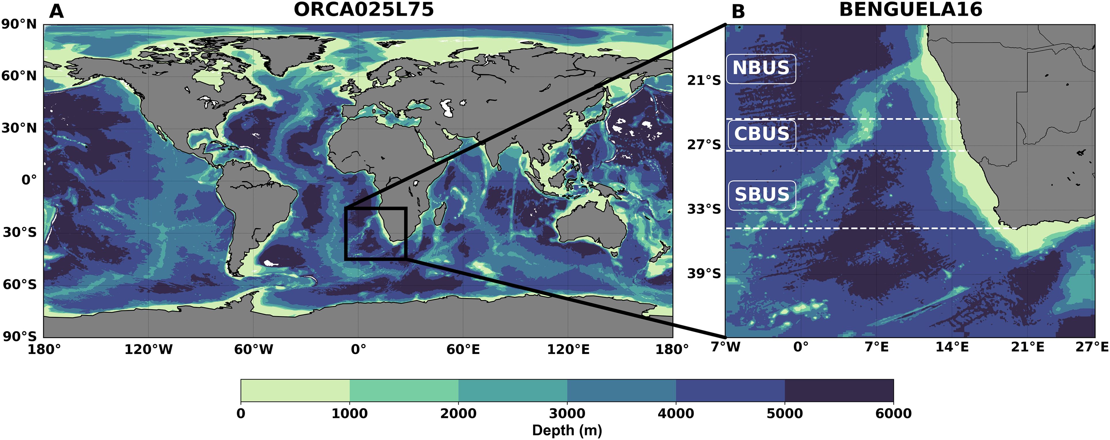
Figure 1. (A) The global ocean ORCA025L75 configuration at 1/4° resolution, and (B) the nested regional domain BENGUELA16 at a resolution of 1/16°. The colormap represents bathymetry derived from the GEBCO dataset (GEBCO Compilation Group, 2021). The right panel shows the subdivision of the Benguela region into northern (NBUS), Central (CBUS), and Southern (SBUS) subregions, with dashed horizontal white lines indicating the boundaris of each.

Compared to other EBUS, the Benguela Upwelling System has received less intense scientific scrutiny throughout time. Furthermore, the lack of high-quality observations in this region has prevented a sound understanding of its internal dynamics (Brandt et al., 2024). As a result, numerical models have become essential tools for researchers working in this region (Penven et al., 2001; Veitch et al., 2009; Chen et al., 2012; Santos et al., 2012; Schmidt and Eggert, 2016; Tomety, 2022), offering both temporal and spatial coverage to complement observational gaps. The BUS represents a peculiar modeling case study due to its pronounced spatial heterogeneity, reflected in contrasting upwelling seasonality and intensity between its subregions. Moreover, the restriction of upwelling events to a narrow coastal band, and the complex circulation patterns pose considerable challenges to any numerical modeling effort.

Several modeling applications were developed to address the physical and biogeochemical dynamics of the Benguela Upwelling System, each facing specific challenges related to four key factors: horizontal spatial resolution, temporal coverage, domain extent, and biogeochemical model complexity. In the early work of Penven et al. (2001), a regional physical model with a one-way nested Benguela subdomain (1/12°) was driven by 1° monthly climatological atmospheric fields. While upwelling events were clearly identified, an overestimated influx of cold water in the upwelling zone was attributed to the low spatiotemporal resolution of the forcing fields. Subsequently, Koné et al. (2005) simulated primary and secondary production in the Benguela ecosystem using two nutrient-phytoplankton-zooplankton-detritus networks with increasing complexity. The more complex ecosystem structure enabled a better representation of the seasonal phytoplankton cycle and nutrient concentrations. The coupled physical-biogeochemical model by Gutknecht et al. (2013) was successfully used to identify the role of large-scale circulation in shaping the ecosystem dynamics of the northern and southern Benguela. However, this application was generally limited to relatively short time windows (up to 15 years), constraining the analysis of long-term variability within the system. The nested physical model developed by Small et al. (2015) demonstrated that increasingly finer horizontal resolution of wind stress fields (up to 0.5°) failed to reproduce realistic upwelling structures unless winds were adjusted toward coastal observations. Schmidt and Eggert (2016) employed a regional high-resolution coupled physical-biogeochemical model, forced by realistic time-varying atmospheric fields, to investigate the impacts of physical and biogeochemical processes on dissolved oxygen dynamics in the BUS over 15 years (1999–2014). More recently, Six and Mikolajewicz (2022) used a global configuration model to show how varying spatial resolution can improve simulations of biogeochemical processes within the BUS.

In light of previous applications, we here present a coupled physical-biogeochemical modeling system for the broader Benguela Upwelling System (northern, central, southern, and Agulhas bank subregions) (Figure 1B), designed to address prior limitations by offering high spatial resolution, expanded temporal coverage, and the use of high-grade atmospheric forcing data. The physical component of the regional BUS modeling system is two-way nested into a general circulation model of the global ocean, allowing for an accurate specification of physical lateral boundary conditions. This solution provides reliable boundary conditions for the regional model, as it allows dynamic feedback from the high-resolution regional domain to the global one by improving the consistency of large-scale dynamics near the regional boundaries (Herzfeld and Rizwi, 2019). Moreover, this approach will ensure that the biogeochemical component will benefit from the improved representation of the physical processes, enhancing the realism of transport dynamics within the system and across the oceanic boundaries. The biogeochemical model component is structured toward an intermediate complexity of lower trophic level interactions, with explicit representation of stoichiometric variability in primary producers, organic matter, and pelagic-benthic interactions. The coupled modeling system was forced with state-of-the-art high-resolution atmospheric reanalysis fields (ERA5) to simulate the BUS dynamics in a temporal extent spanning four decades (namely 1980–2020) and outcomes were validated against multiplatform observational datasets. This modeling framework is employed to simulate key environmental features of the Benguela Upwelling System under changing climate conditions, with a focus on the interplay between upwelling dynamics and the spatio-temporal variability of marine productivity. The validated system enables the investigation of long-term changes in sea surface temperature and upper ocean Chl-a, providing insight into the BUS’s response over four decades.

The following section provides a detailed description of the coupled modeling framework, followed by an evaluation of the simulated BUS dynamics over the study period using observational datasets encompassing both physical and biogeochemical parameters. A thorough discussion of the results is then provided, leading to the conclusions of the study.

2 Coupled physical-biogeochemical modeling system

2.1 Physical component

The ocean’s general circulation is simulated using the open-source “Nucleus for European Modelling of the Ocean” (NEMO v.4.2.2; Madec and the NEMO System Team, 2023). This three-dimensional, finite-difference ocean model solves the Navier-Stokes primitive equations and employs a non-linear equation of state that couples active tracers with fluid velocity, following hydrostatic and Boussinesq assumptions.

The physical component of the modeling system is constituted by a global ocean configuration that utilizes a global ORCA tripolar grid (Madec and Imbard, 1996) with a nominal horizontal resolution of 1/4° (~27.75 km) at the equator, refining to approximately 14 km at 60° latitude. A regional domain representing the BUS is nested within the global configuration using the “Adaptive Grid Refinement in Fortran” tool (AGRIF; Debreu et al., 2012). This regional domain achieves a higher horizontal resolution of 1/16° (~7 km) and extends from 15.71°S to 44.89°S and from 7.03°W to 27.28°E (Figures 1A, B). A two-way nesting method is adopted, enabling the regional configuration to receive lateral open boundary conditions from the global one, whose physical fields are then improved by means of the regional high-resolution oceanic conditions. Herein, the global configuration is referred to as ORCA025L75 and the regional configuration as BENGUELA16. Both configurations share the same vertical z-coordinate system, consisting of 75 layers ranging from a few meters near the surface to approximately 200 meters in the deep ocean. Data from the General Bathymetric Chart of the Oceans grid (GEBCO; GEBCO Compilation Group, 2021) were used to generate the bathymetry of each configuration.

Vertical mixing is parameterized using the turbulent kinetic energy scheme (Blanke and Delecluse, 1993), while the advection of active tracers (temperature and salinity) is computed using a total variance dissipation scheme, and the lateral mixing is applied through a Laplacian formulation along iso-neutral surfaces. Bottom friction is modeled using a quadratic formulation. In the global configuration, additional parameterizations account for the subgrid-scale vertical mixing and the diffusive bottom boundary layer. Momentum and heat exchange at the air-sea interface are simulated through the ECMWF bulk parameterization scheme (Brodeau et al., 2017), while near-surface atmospheric forcing data were obtained from the ERA5 reanalysis dataset (Hersbach et al., 2020), which has a horizontal resolution of 31 km and an hourly frequency. A spatially explicit, time-invariant geothermal heat flux is prescribed at the seafloor using data from Goutorbe et al. (2011). Riverine freshwater inputs are derived from the Global Flood Awareness System reanalysis (GloFAS v2.1; Alfieri et al., 2013), setting as inputs values zero salinity and the same temperature of the corresponding ocean grid-point.

A spin-up simulation is conducted by repeating the forcing conditions from 1980 over 15 annual cycles. The initial three-dimensional temperature and salinity fields are obtained from the 1981–2010 climatology of the World Ocean Atlas 2018 (Locarnini et al., 2018; Zweng et al., 2019). Temperature and salinity are not restored toward surface reference fields. The time integration of the ocean model is performed with a timestep of 1200 s for the global configuration and 400 s for the regional one. The final physical state at the end of the spin-up period serves as the initial condition for a 41-year hindcast simulation, covering the period from January 1980 to December 2020.

2.2 Biogeochemical component

The biogeochemical component is provided by the “Biogeochemical Flux Model” (BFM v.5.3; Vichi et al., 2023). BFM is an open-source, community-developed, generic biomass-based marine biogeochemical model. It represents the system in Eulerian coordinates, simulating the pelagic dynamics of the marine ecosystem through a suite of chemical and biological processes. The pelagic-benthic coupling is implemented via a simple benthic closure, where fixed quotes of the sedimented organic matter are remineralized and returned to the water column as nutrients.

The model organizes elemental components—carbon, nitrogen, phosphorus, silicon, iron, and oxygen—into chemical functional families, forming the structural elements of both living functional groups and non-living organic matter. Biogeochemical cycling is solved independently for the following dissolved components: nitrate (NO₃^-), ammonium (NH₄⁺), phosphate (PO₄^3-), silicate (SiO₄^4-), iron (Fe), and oxygen (O₂). The ocean carbonate system is modeled with dissolved inorganic carbon (DIC) and total alkalinity as prognostic state variables, following the best practices outlined by Orr et al. (2017). The lower-trophic level ecosystem interactions represented in this study by the BFM can be considered of intermediate complexity (see, e.g., Lovato and Butenschön, 2023). The ecosystem structure accounts for five living functional groups: heterotrophic bacteria, two phytoplankton groups (diatoms and nanoflagellates), and two zooplankton groups (microzooplankton and mesozooplankton). A schematic diagram illustrating the relationships and interactions between the different model components is provided in Figure 2.

Figure 2

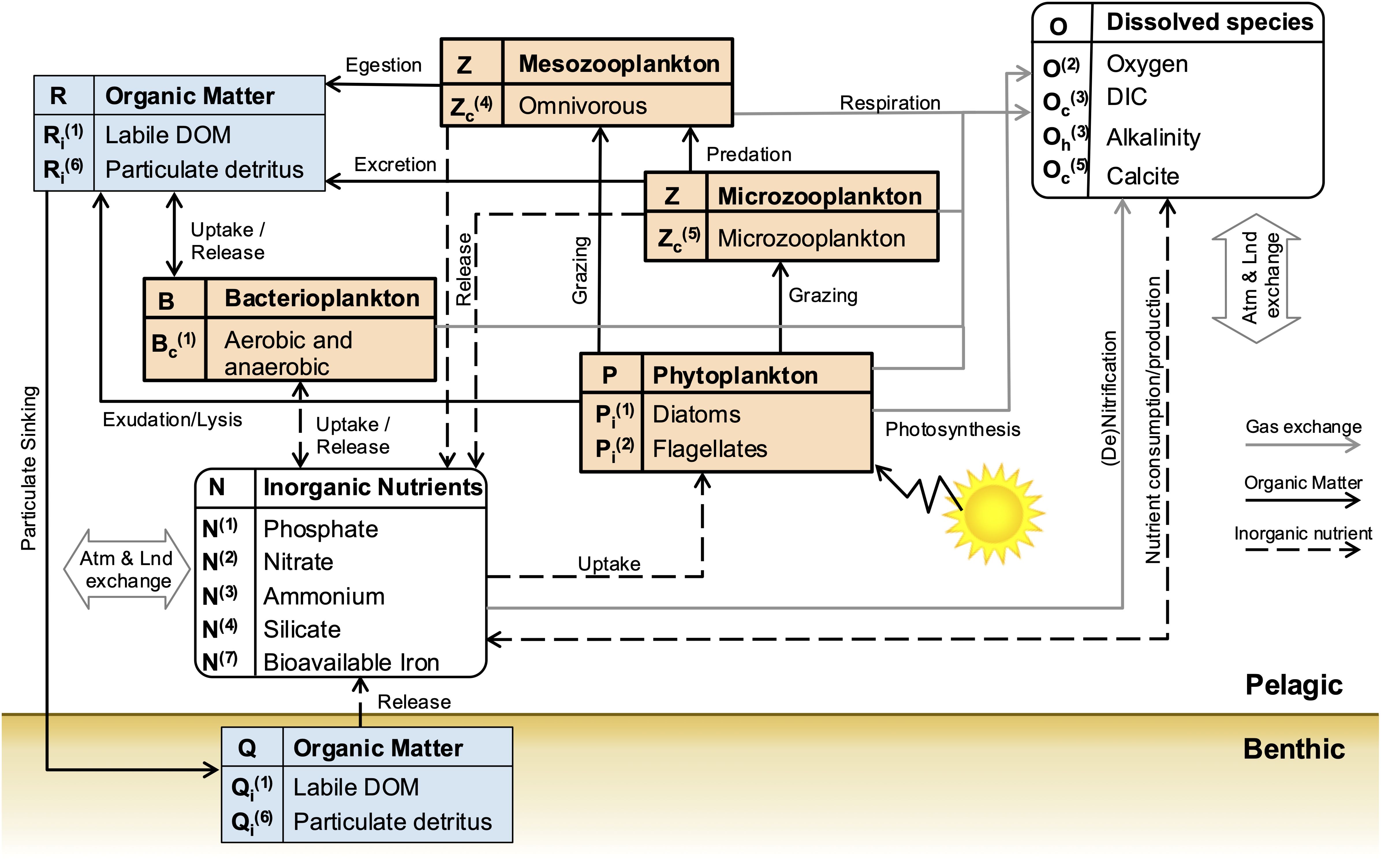
Figure 2. Schematic representation of the lower trophic level ecosystem structure used for the BENGUELA16 configuration of the BFM model. Living Functional Groups are represented by bold-line square boxes, non-living Functional Groups by thin-line square boxes, and inorganic components by rounded boxes. Black dashed lines indicate the flow of inorganic nutrients, solid black lines the flow of organic matter, and the gray solid lines the gas exchanges. The subscript i in the component’s short names denotes the selected Chemical Functional Families (C, N, P, Si, Fe,…). Double arrows indicate the exchanges at the boundaries with atmospheric and land systems.

The coupling between the physical and biogeochemical components of the modeling system is achieved through an offline procedure, utilizing high-frequency physical fields previously computed for the BUS regional configuration. These data are processed by the NEMO interface “Tracers in Ocean Paradigm” (TOP; Aumont et al., 2019) to resolve the advective and diffusive transport of biogeochemical tracers, while reaction terms computed by the BFM are integrated using a source-splitting method (see details in Lovato and Butenschön, 2023). The advection of passive tracers is solved using the monotonic upstream scheme for conservative laws (MUSCL), while lateral diffusion follows the same approach used for physical active tracers. A key advantage of the offline coupling procedure is the ability to use a longer integration timestep which was set to 900 s.

Similar to the physical component, a spin-up simulation of marine biogeochemical quantities was conducted for 15 years by repeatedly applying the physical circulation fields of the year 1980. Initial conditions for O₂, SiO₄^4-, PO₄^3-, and NO₃^- were derived from the World Ocean Atlas 2018 (WOA18; Garcia et al., 2019a, 2019b), while total alkalinity and dissolved inorganic carbon concentrations were sourced from the climatological gridded dataset of the Global Ocean Data Analysis Project (GLODAP v2; Lauvset et al., 2022). All other variables were initialized with uniform values in the upper ocean (0–100 m), as described in Orr et al. (2017). Climatological river nutrient loads were prescribed using fields produced by the Global Nutrient Export from Watersheds 2 model (NEWS2; Mayorga et al., 2010). Lateral open boundary conditions for biogeochemical variables were obtained from monthly fields generated in the historical and ssp245 experiments by the CMCC-ESM2 model (Lovato et al., 2023a, 2023b).

After the spin-up simulations, the regional BUS configuration was used to simulate the evolution of marine biogeochemistry over the period 1980–2020.

2.3 Observational datasets

A comprehensive set of multiplatform observational datasets, including global gridded products and local in-situ measurements, was used to assess the performance of the coupled modeling system.

Global scale gridded datasets employed in the validation of marine physics accounted for three main seawater parameters, namely temperature, salinity, and near-surface current speed. Satellite-derived data products from the European Space Agency-Climate Change Initiative (ESA-CCI) comprised the sea surface temperature (SST, Merchant et al., 2019) at 5 km of spatial resolution over the period 1982–2020 and the sea surface salinity (SSS, Boutin et al., 2021) covering the years range 2010–2019 with a nominal resolution of 25 km. Reference fields of the near-surface (15 meters depth) current velocities were obtained from the Ocean Surface Current Analyses Real-time (OSCAR) from 2012 to 2020 and with a third of degree (~37 Km) horizontal resolution (ESR, 2009). The subsurface ocean validation of three-dimensional temperature and salinity fields was addressed using the multi-observation global ocean ARMOR3D analysis at a resolution of 25 km (CMEMS, 2022), which merges in-situ and satellite observations over the 1993–2020 period using multiple linear regression methods that relate surface and subsurface data (Guinehut et al., 2012).

The validation of the biogeochemical component focused on dissolved inorganic nutrients (NO₃^- and PO₄^3-), dissolved oxygen, and Chl-a from either gridded climatologies or in-situ datasets. Annual climatological data of dissolved oxygen, NO₃^-, and PO₄^3- were sourced from the CSIRO Atlas of Regional Seas (CARS, 2009), at half a degree (~55 Km) of horizontal resolution and over 79 depth levels, with vertical intervals ranging from 5 m near the surface to 250 m at deep layers. Upper ocean Chl-a concentrations were obtained from satellite observations based on the Copernicus-GlobColour processor, using the Garver-Siegel-Maritorena (GSM) algorithm, covering the period 1998–2020 at a resolution of 4 km (CMEMS, 2023).

In-situ observations were retrieved from different sampling cruises and monitoring platforms, as illustrated in Figures 3A, B. Dissolved inorganic nutrients (NO₃^- and PO₄^3-) profiles come from two oceanographic cruises. The RV James Cook cruise (JC032) held in April 2009, conducted at a latitudinal transect near 24°S, extending longitudinally from 6°W to 14°E, including 23 vertical profiles, each with approximately 24 depth levels from the surface down to 5500 m depth (Schuster et al., 2013). The RV Africana cruise (Afr258) in December 2009 accounts for 16 profiles along the Benguela coastal zone between 17°S and 33°S (Rixen and Flohr, 2012; Flohr et al., 2014).

Figure 3

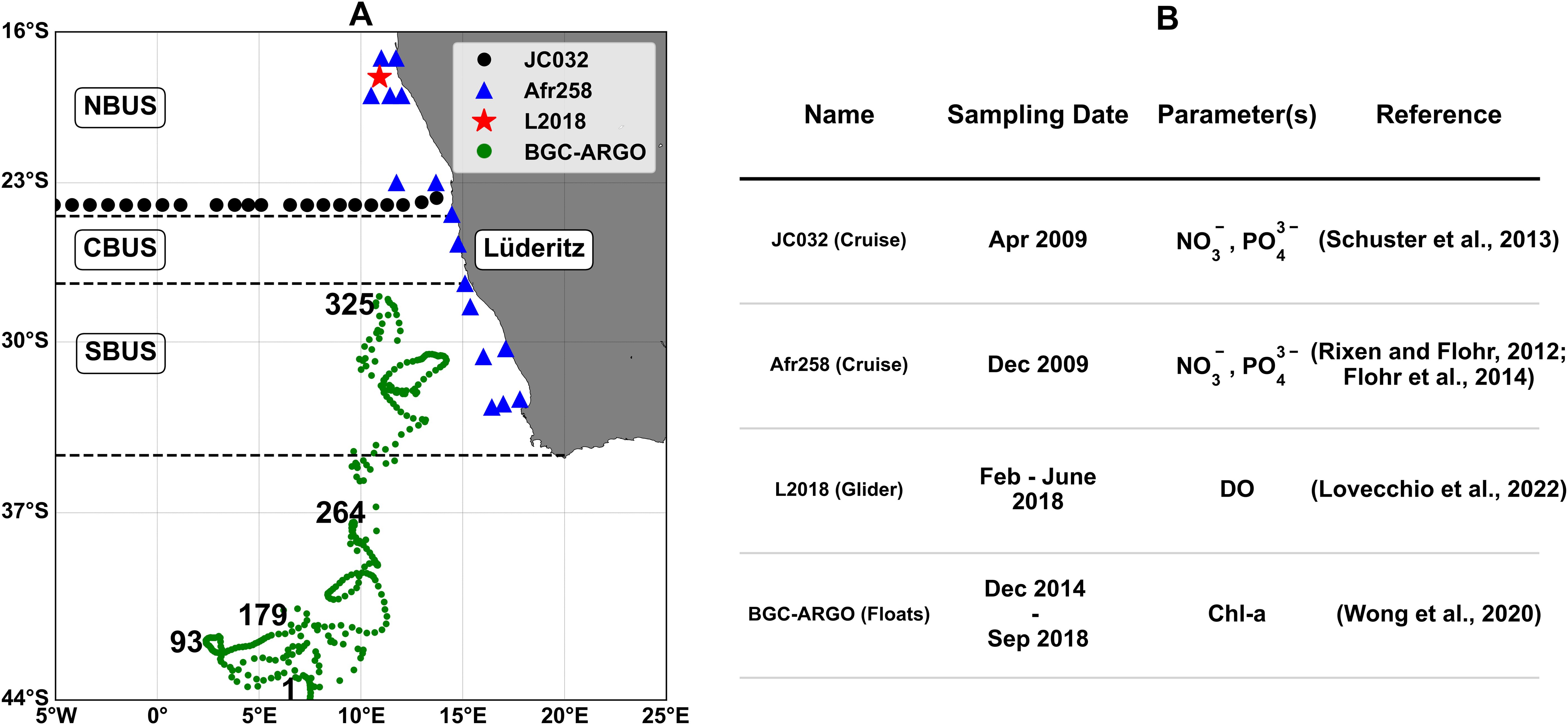
Figure 3. Location (A) and source details (B) of the diverse in-situ measurements collection used to validate the BENGUELA16 biogeochemical component. NBUS, CBUS, and SBUS refer respectively to the Northern, Central, and Southern Benguela subregions. The green dots represent the BGC-ARGO observations profiles (Wong et al., 2020), where labels indicate the prospective locations of the float over time.

Chl-a vertical distribution was assessed using 325 profiles collected by Biogeochemical Argo (BGC-ARGO) float number 6901582 between December 2014 and September 2018 in the open waters of the southern Benguela subregion, extending from the surface to 1000 m of depth (Wong et al., 2020). Daily dissolved oxygen observations were derived from a high-resolution glider deployed from February to June 2018 in the NBUS (Lovecchio et al., 2022). The glider followed a ~12 km triangular path and profiled to 1000 m depth with ~20 cm vertical resolution, surfacing 5–6 times daily and sampling primarily on upward dives.

3 Results

This section presents the validation of the model simulations, providing a concise assessment of the global ORCA025L75 physical component and a more detailed evaluation of the BENGUELA16 regional domain. The comparison with climatological gridded datasets aims to evaluate the presence of systematic spatial biases in the long-term mean state simulated by the model across the different BUS subregions, while the comparison with discrete in-situ measurements assesses the capability of the modeling system to realistically capture observed spatio-temporal features.

Overall model performance is evaluated using spatial bias (Model - Observations), normalized standard deviation (STD), normalized root mean square difference (RMSD), and the correlation coefficient (r). The latter three metrics are visualized using a normalized Taylor diagram (Jolliff et al., 2009), where the azimuthal angle represents the correlation coefficient, the radial distance indicates the normalized standard deviation, and the RMSD is shown as the distance from the reference point on the x-axis labeled “OBS”. This point represents an ideal agreement between the model and observations, with a correlation coefficient and normalized STD equal to 1 and an RMSD of zero. Closer proximity to this point indicates better model performance relative to observations.

Observational gridded datasets were interpolated onto the model grid, with 2D datasets adjusted horizontally and 3D datasets interpolated both horizontally and vertically. In-situ observations were compared with simulated values at the nearest grid point and corresponding time frame. Linear trends from both the model and observations are computed using classical least squares regression for each calendar month and for the Benguela subregions, based on the latitudinal boundaries shown in Figure 3A.

3.1 Validation of global ocean physical fields (ORCA025L75)

A brief description of the main physical results from the global ocean configuration is provided here to complement the overall modeling system assessment, with a focus on the reliability of the simulated fields in the South Atlantic region surrounding the Benguela upwelling area.

The global ocean configuration ORCA025L75 demonstrates satisfactory skill in reproducing the annual climatology of SST patterns when compared to ESA-CCI satellite observations (Figures 4A–C). The model accurately captures the horizontal distribution of SST, with a spatial mean bias of about 0.02 °C. However, localized positive biases of approximately 3 °C are evident along western boundary current regions, where strong horizontal circulation patterns exhibit substantial variability. Seasonal patterns of SST climatological fields are also fairly well represented by the model (Supplementary Figure S1), with mean seasonal biases ranging from 0.11 °C in austral summer (DJF) to -0.05 °C in austral spring (September to November, SON). A quantitative evaluation of the 3D temperature climatology is conducted using a normalized Taylor diagram (Figure 5A), compared against ARMOR3D data. Both annual and seasonal climatological values consistently cluster below 0.40 RMSD and show remarkably high positive correlation coefficients exceeding 0.95 across all depth ranges. The close agreement between ORCA025L75 and ARMOR3D is further supported by the proximity of normalized STD values, indicating the model effectively captures the amplitude of variability in observed data.

Figure 4

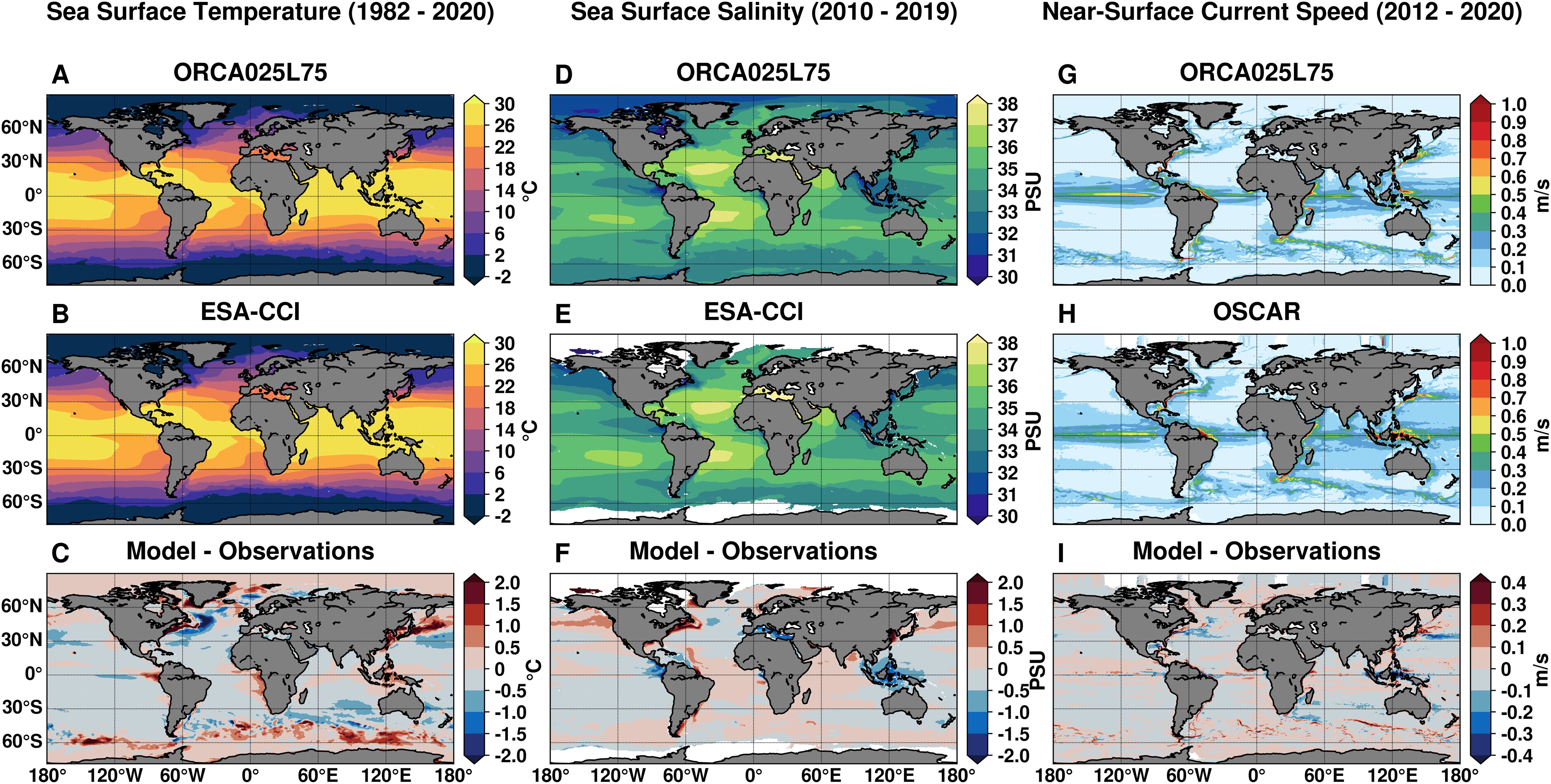
Figure 4. Long-term average climatological fields for sea surface temperature (A–C), sea surface salinity (D–F), and near-surface current speed at 15 m depth (G–I). For each variable, panels show output from the ORCA025L75 (A, D, G), corresponding observational datasets from ESA-CCI (B, E) and OSCAR (H), and the model–observation differences (C, F, I).

Figure 5

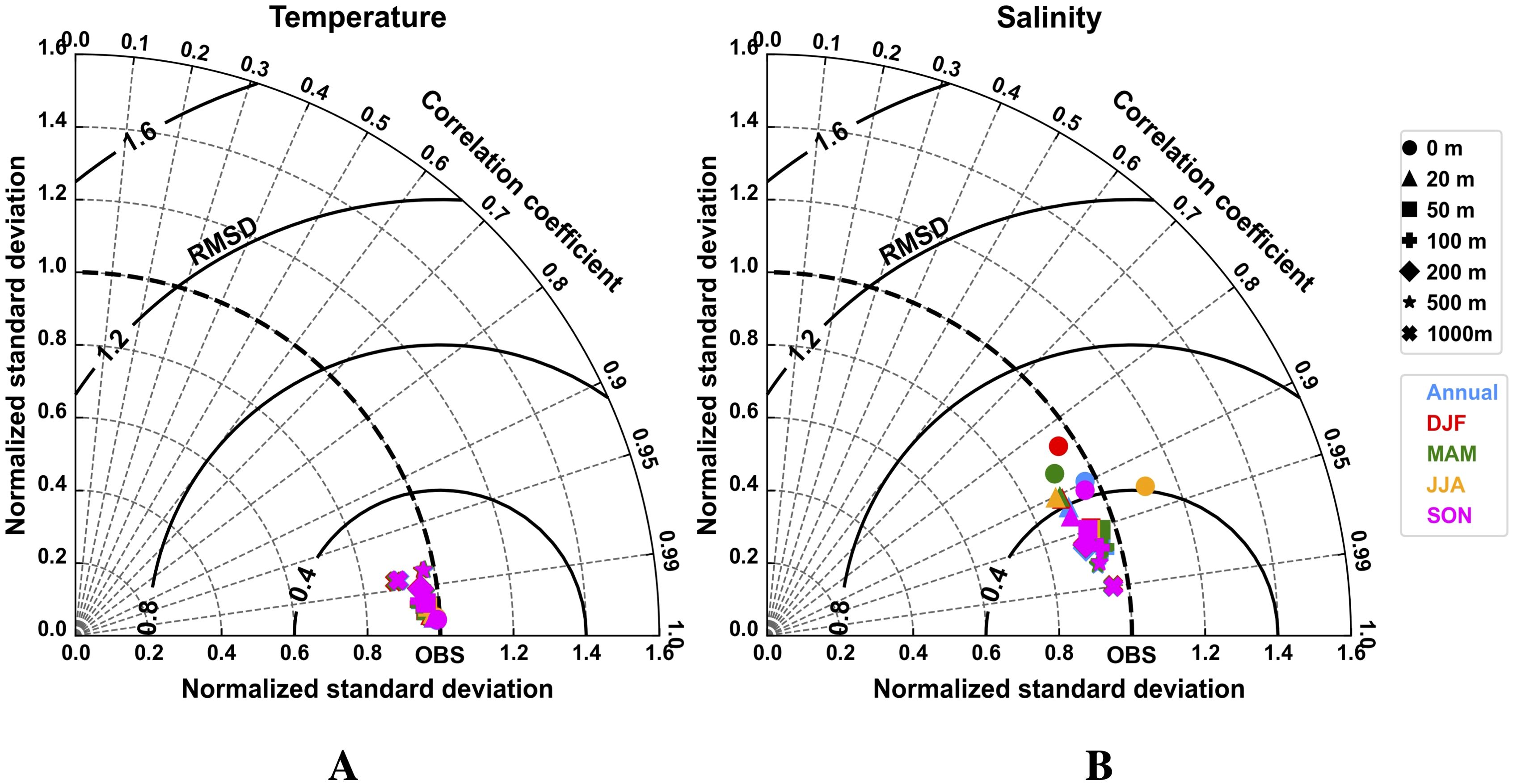
Figure 5. Normalized Taylor diagrams summarizing the comparison of climatological (1993–2020) seawater temperature (A) and salinity (B) fields from the ORCA025L75 physical simulation and the ARMOR3D analysis (CMEMS, 2022). Symbols refer to different depth levels, while colors indicate both annual and seasonal mean values. Each Taylor diagram reports the correlation coefficient (azimuthal angle; gray dashed lines), normalized standard deviation (radial distance), and root-mean-square difference (RMSD; bold black contours).

The comparison of simulated SSS annual climatology with ESA-CCI satellite observations (Figures 4D–F) also reveals a rather good agreement, with a spatial mean bias of approximately -0.03 PSU and seasonal differences ranging from -0.04 to -0.02 PSU in JJA and DJF, respectively (Supplementary Figure S2). Nonetheless, the comparison highlights both positive and negative SSS biases near river mouths. In the vicinity of the BUS, the SSS bias remains minimal, within ±0.50 PSU (Figures 4D–F). The normalized Taylor diagram (Figure 5B) shows that values are more scattered in near-surface layers than at depth, with RMSD values below 0.50 and generally high positive correlations (> 0.80) in most instances.

Annual climatological fields of near-surface (15 m depth) horizontal current speeds, as simulated by ORCA025L75, are compared with OSCAR analysis data (Figures 4G–I). Mean biases remain well below -0.01 m/s, and the model effectively reproduces the main patterns of oceanic circulation. However, notable deviations are observed primarily in the equatorial band and along western boundary currents, consistent with the SST bias patterns.

Overall, the mean oceanic physical conditions simulated by the global component of the modeling system are characterized by relatively modest biases in the South Atlantic region surrounding the Benguela upwelling area, helping to provide improved boundary conditions.

3.2 Benguela regional model validation (BENGUELA16)

3.2.1 Marine physics

The performance of the physical component in the BENGUELA16 domain was assessed by comparing long-term climatological surface fields with satellite-derived observations and analysis datasets (Figure 6). The simulated data exhibit low mean spatial biases for SST, SSS, and near-surface current speed, with respective values of -0.10 °C, 0.04 PSU, and 0.02 m/s. Compared to ESA-CCI SST data (Figures 6A–C), the BENGUELA16 physical component correctly reproduces the influx of warm water into the Atlantic Ocean via the Agulhas Current around the southern tip of Africa, as well as the warm water intrusion from the Angola-Benguela frontal zone along the northern boundary of the BUS. The model reliably simulates the presence of cold water masses along the Namibian coastal shelf, which indicates the underlying coastal upwelling process. The SST bias along the coastal area remains relatively modest, around 0.53° C, where the simulated upwelling dynamics determine the spatial shape and extent of the surface temperature gradient toward the open ocean. These biases become more pronounced in the seasonal climatology (Supplementary Figure S3), varying across different regions of the BUS in response to dominant circulation patterns.

Figure 6

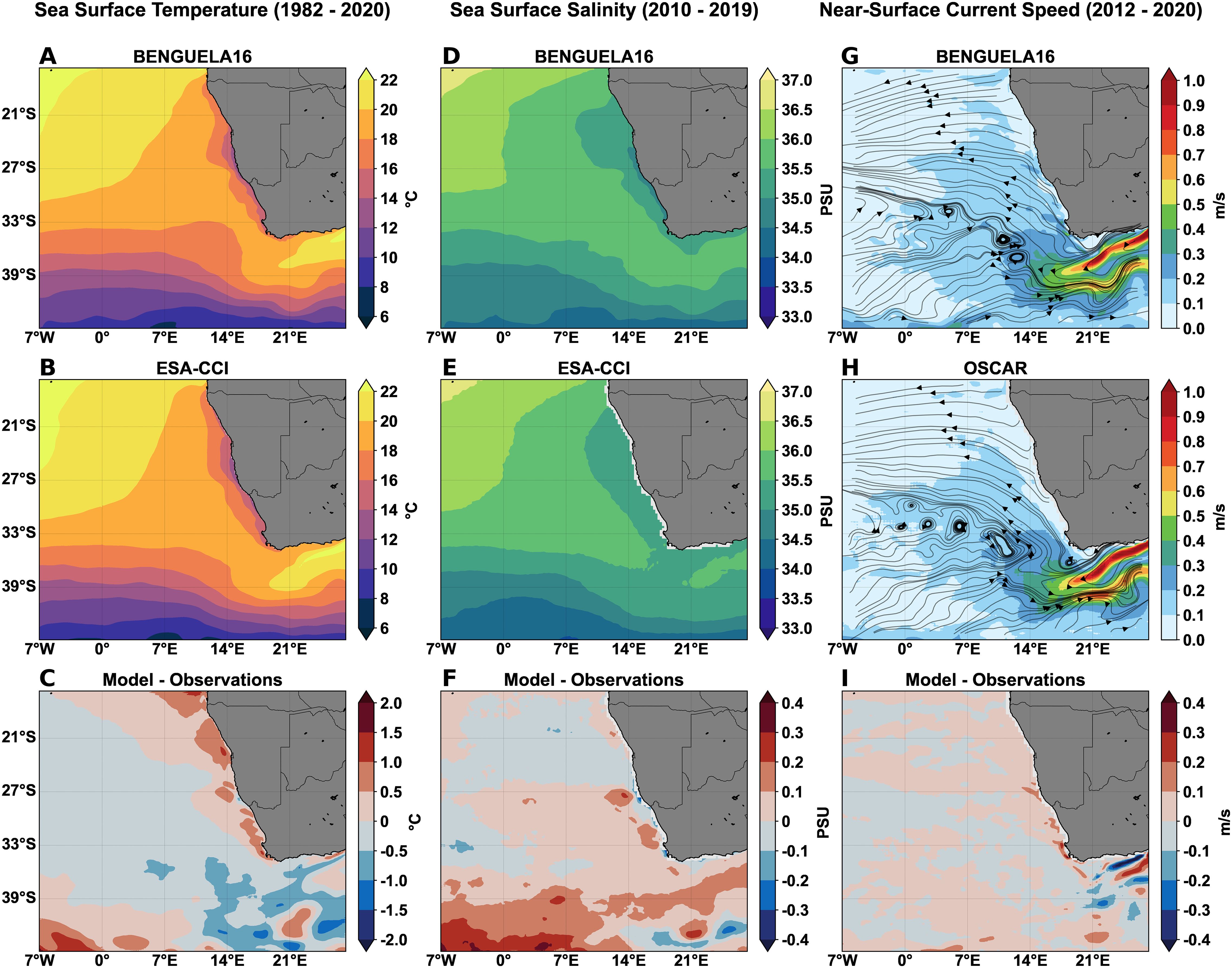
Figure 6. Long-term average climatological fields for sea surface temperature (A–C), sea surface salinity (D–F), and near-surface current speed at 15 m depth (G–I). For each variable, panels show output from the BENGUELA16 (A, D, G), corresponding observational datasets from ESA-CCI (B, E) and OSCAR (H), and the model–observation differences (C, F, I). Streamlines in (G, H) represent circulation directions at 15 meters, where lines were subsampled every 10 grid points to enhance plotting clarity.

Similarly, the BENGUELA16 model reproduces the low-salinity waters bordering the Namibian shelf, as observed in the ESA-CCI dataset (Figures 6D–F), with an absolute difference of 0.10 PSU, and the seasonal fields exhibit a remarkably variable spatial distribution of biases (Supplementary Figure S4). The comparison of near-surface horizontal current speeds (Figures 6G–I) indicates minimal biases. Both the location and the extent of major circulation features, including the Agulhas Current and its retroflection, are satisfactorily reproduced by the physical component and minimal deviations occurred only in the approaches of the coastal eastern boundary.

For subsurface temperature and salinity, the model’s performance was evaluated by comparing long-term climatological fields with the ARMOR3D dataset at selected depth levels (Figures 7A, B). These Taylor diagrams indicate that across all examined depth levels and temporal windows, RMSD values remain below 0.40 and correlation coefficients are consistently high (> 0.90) for both variables. In particular, salinity data are closely clustered near the reference value, while temperature shows a slight decrease in correlation at 1000 m depth.

Figure 7

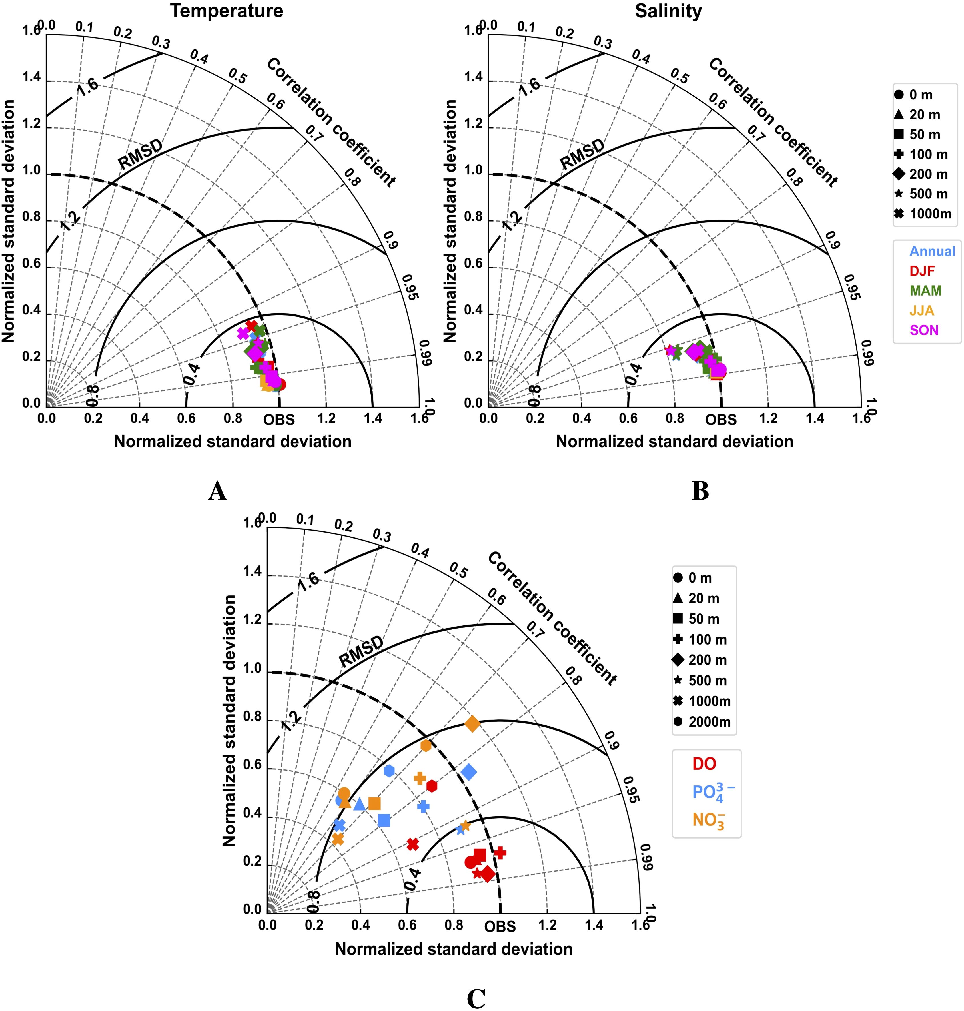
Figure 7. Normalized Taylor diagrams summarizing the comparison of climatological seawater temperature (A), seawater salinity (B), and diverse biogeochemical fields (C) from the BENGUELA16 simulation averaged over the period 1993–2020 against the physical data form ARMOR3D analysis (CMEMS, 2022) and CARS climatological data (CARS, 2009). Biogeochemical data shown in panel (C) refer to dissolved oxygen (DO), dissolved inorganic phosphate (PO₄^3-), and dissolved inorganic nitrate (NO₃^-). Symbols indicate different depth levels, while colors in panels (A–B) indicate annual and seasonal averages. Each Taylor diagram reports the correlation coefficient (azimuthal angle; gray dashed lines), normalized standard deviation (radial distance), and root-mean-square difference (RMSD; bold black contours).

The same annual climatological fields were used to represent the vertical distribution of seawater temperature and salinity down to ~800 m along a longitudinal section in the central BUS region at 26.64°S (Figures 8A, B). The persistence of the upwelling process reflects on the isotherms and isohalines tilting up and outcropping near the coastal area, as clearly visible in both simulated and observational fields. This upwelling-induced deformation of isolines extends down to approximately 400 m. However, notable biases emerge mostly in the upper 200 m along a narrow coastal strip, where the simulated fields exhibit a sharper gradient toward coastal waters compared to the smoother ARMOR3D fields.

Figure 8

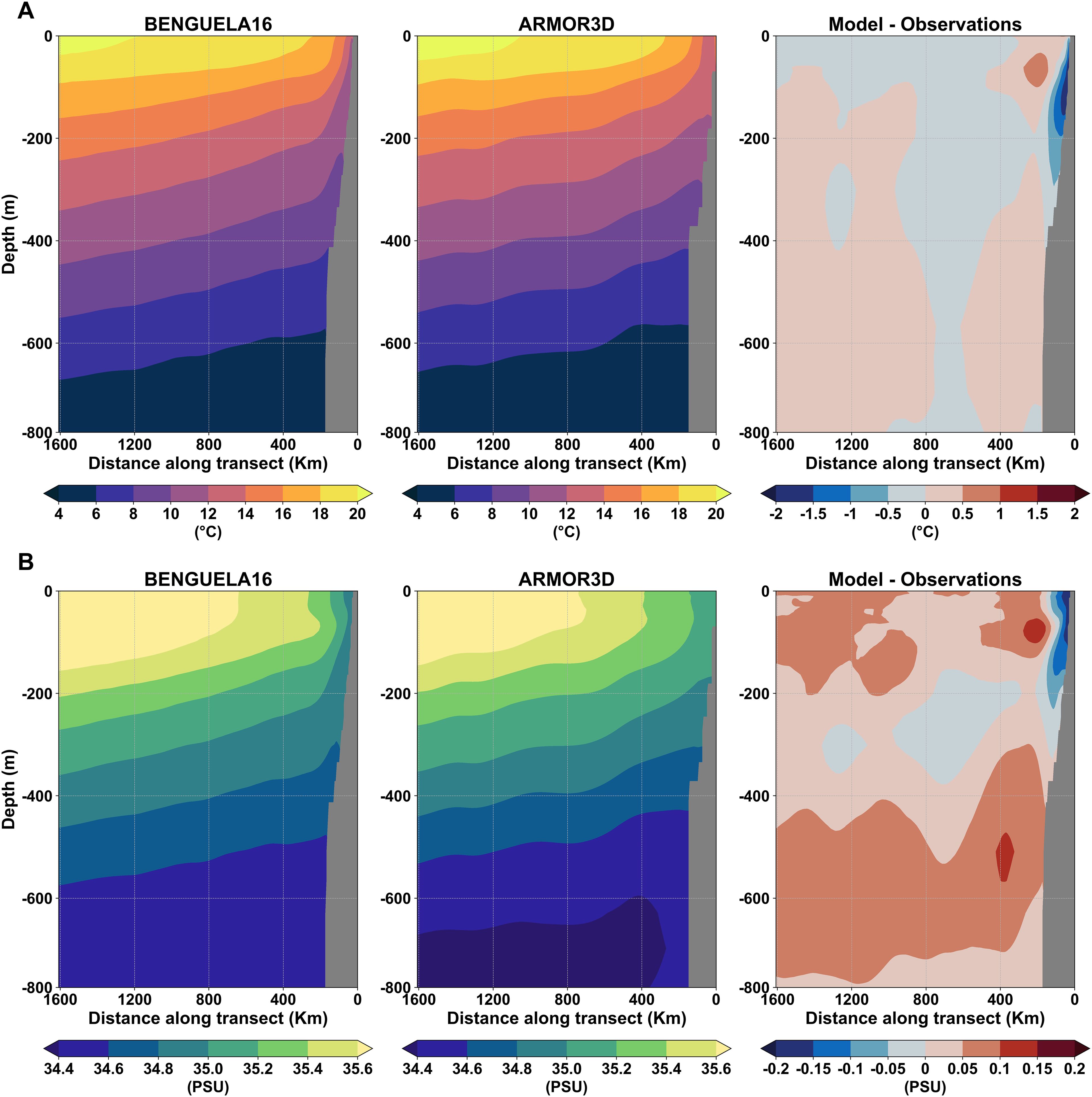
Figure 8. Seawater temperature (A) and salinity (B) climatological fields (1993-2020) along a longitudinal section at approximately 26.64°S, derived from the BENGUELA16 simulation (left panel), ARMOR3D analysis (CMEMS, 2022) (center), and their differences (right).

3.2.2 Marine biogeochemistry

The validation of the BENGUELA16 biogeochemical component is presented here through comparison with gridded and in-situ observational datasets (see Section 2.3) of seawater concentrations for dissolved inorganic nitrate and phosphate, dissolved oxygen, and Chl-a.

Gridded climatological data for dissolved inorganic nitrate and phosphate from the CARS dataset were compared with the BENGUELA16 long-term climatology (1980–2020), using spatial statistical metrics across eight different depth levels (Figure 7C). The spatial distribution of inorganic nutrients shows adequate correlation with observational data at all depths, with values ranging from 0.60 to 0.90, indicating that the model effectively captures the distribution of these inorganic nutrients. However, accuracy decreases in subsurface layers, where RMSD values for NO₃^- reach approximately 0.80. PO₄^3- shows smaller variations, with lower RMSD values at shallower depths (e.g., 50, 100, and 200 meters) and higher values in deeper layers (1000 and 2000 meters). Notably, the surface layer exhibits an RMSD of ~0.80.

The reliability of the simulated monthly averaged vertical distribution of NO₃^- and PO₄^3- was assessed using 16 in-situ profiles from the Afr258 cruise in December 2009 and 27 casts from the JC023 cruise along a longitudinal transect in April 2009 (Figures 9A, B). Model data were extracted at the nearest grid cells and time frame, and vertically interpolated to match the depth levels of observations. The linear correlations for both nutrients were high and statistically significant (p-value < 0.05), although localized spatial differences were evident. In deeper layers (500–1500 m), NO₃^- data pairs align well in the NBUS sub-region, while PO₄^3- shows slightly lower agreement. At intermediate depths (100–500 m), BENGUELA16 systematically underestimates concentrations across all subregions, with average differences of -2.9 mmol N/m³ for NO₃^- and -0.50 mmol P/m³ for PO₄^3-. In the uppermost layers (0–100 m), observations display a widespread, with larger differences in NO₃^- at higher concentrations, whereas PO₄^3- near-surface concentrations show better agreement across all BUS subregions. The comparison with JC023 transect data (Figures 9C, D) is particularly strong, as both longitudinal and vertical variability are well represented by the BENGUELA16 model. The model closely reproduces observed ranges of dissolved inorganic nitrate (0–10 mmol N/m³) and phosphate (0–0.50 mmol P/m³) in the upper 200 meters, effectively capturing both the nutrient-rich coastal upwelling signature and the deep nutrient-rich layer (600–1000 meters). Statistical metrics were computed by extracting model data in correspondence with the JC023 sample locations, showing correlation coefficients of 0.97 for NO₃^- and 0.98 for PO₄^3-, with corresponding RMSE values of 3.65 mmol N/m³ and 0.23 mmol P/m³, respectively.

Figure 9

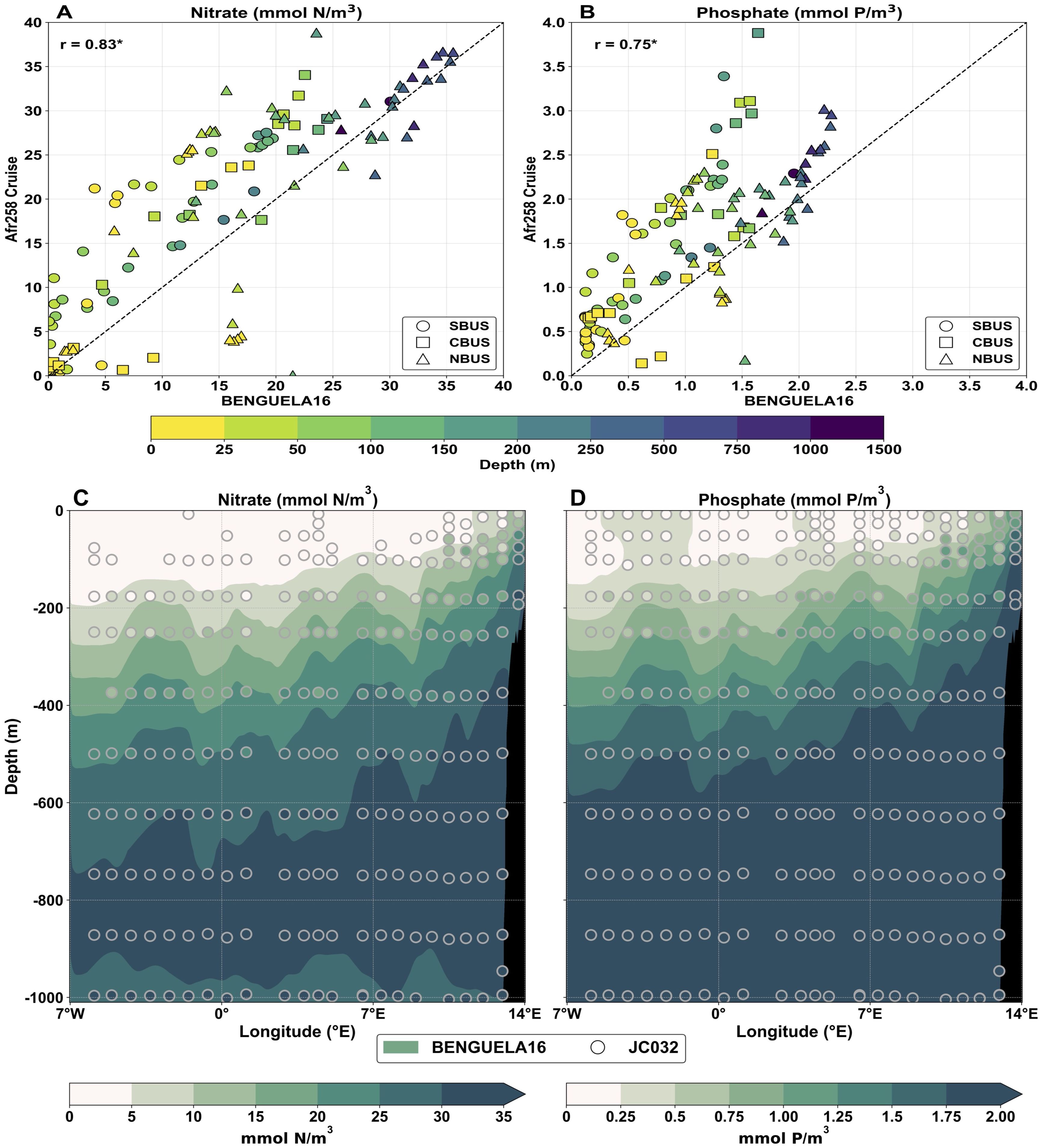
Figure 9. Comparison of BENGUELA16 monthly averaged data for dissolved inorganic nitrate and phosphate against in-situ measurements from Afr258 (A, B) and JC032 (C, D) cruises (see Figure 3 for details). In the top panels, the unequally spaced color scale indicates the depth of samples, while different subregions are associated with symbols. Model data were extracted at the nearest grid cell and sampling date, with values linearly interpolated at the same in-situ sample depths. The dashed line indicates the ideal fit and the Pearson’s correlation coefficient (r) is marked with an asterisk if statistically significant (p < 0.05). In the bottom panels, the BENGUELA16 data were extracted along a longitudinal section at about 24°S which reflects the JC032 cruise path without using any interpolation procedure.

The annual climatological fields of dissolved oxygen show good agreement with CARS data across most depth levels (Figure 7C), with low RMSD and normalized STD values, although correlation coefficients slightly decrease below 500 meters. A more detailed depth-resolved analysis of DO biases (Supplementary Figure S5) shows that the model matches observational data well in upper layers, except near the coast. At 100 meters, notable differences appear along the Benguela coastal region, with negative biases in the north and positive ones in the south. In deeper layers, pronounced negative biases are found at 500 and 1000 meters, particularly along the western lateral open boundary. A direct comparison between time-averaged vertical profiles from high-resolution glider data (February–June 2018) and daily averaged model outputs is presented in Figure 10. The mean vertical profiles align closely, with good agreement in standard deviation ranges in the upper and 400–1000 meter depth range. Simulated minimum and maximum DO values fall within observed ranges, although a bias of about 30 mmol O₂/m³ is evident near 200 meters.

Figure 10

Figure 10. Vertical profiles of the mean and standard deviation range (left panel) and minimum-maximum interval (right panel) computed between February and June 2018 from daily dissolved oxygen glider data (black) and daily BENGUELA16 simulation (red). Model data were extracted at the nearest grid point with respect to the glider reference location (see details in Figure 3A).

Long-term climatological fields of upper ocean Chl-a from BENGUELA16 were compared with Copernicus-GlobColour satellite estimates over the period 1998–2020 (Figure 11). Model-derived satellite-like Chl-a values were computed following the formulation in Vichi et al. (2023). The analysis focused on the upwelling-driven algal bloom extent, defined as the coastal region extending 1000 km offshore (see e.g., Lamont et al., 2019; Hendry et al., 2021). The annual climatological spatial distribution of Chl-a (Figure 11A) shows good agreement with observations, especially across the zonal extent of the coastal Chl-a plume. Despite a slightly negative mean bias (-0.05 mg/m³), differences appear along the narrow coastal band in all BUS subregions, particularly where Chl-a peaks at 5 mg/m³. A scatter plot of model versus satellite grid points (Figure 11B) shows homogeneous clustering in the northern and central subregions, while the southern subregion exhibits two distinct clusters reflecting both positive and negative biases. This difference is also evident in the subregional correlation coefficients.

Figure 11

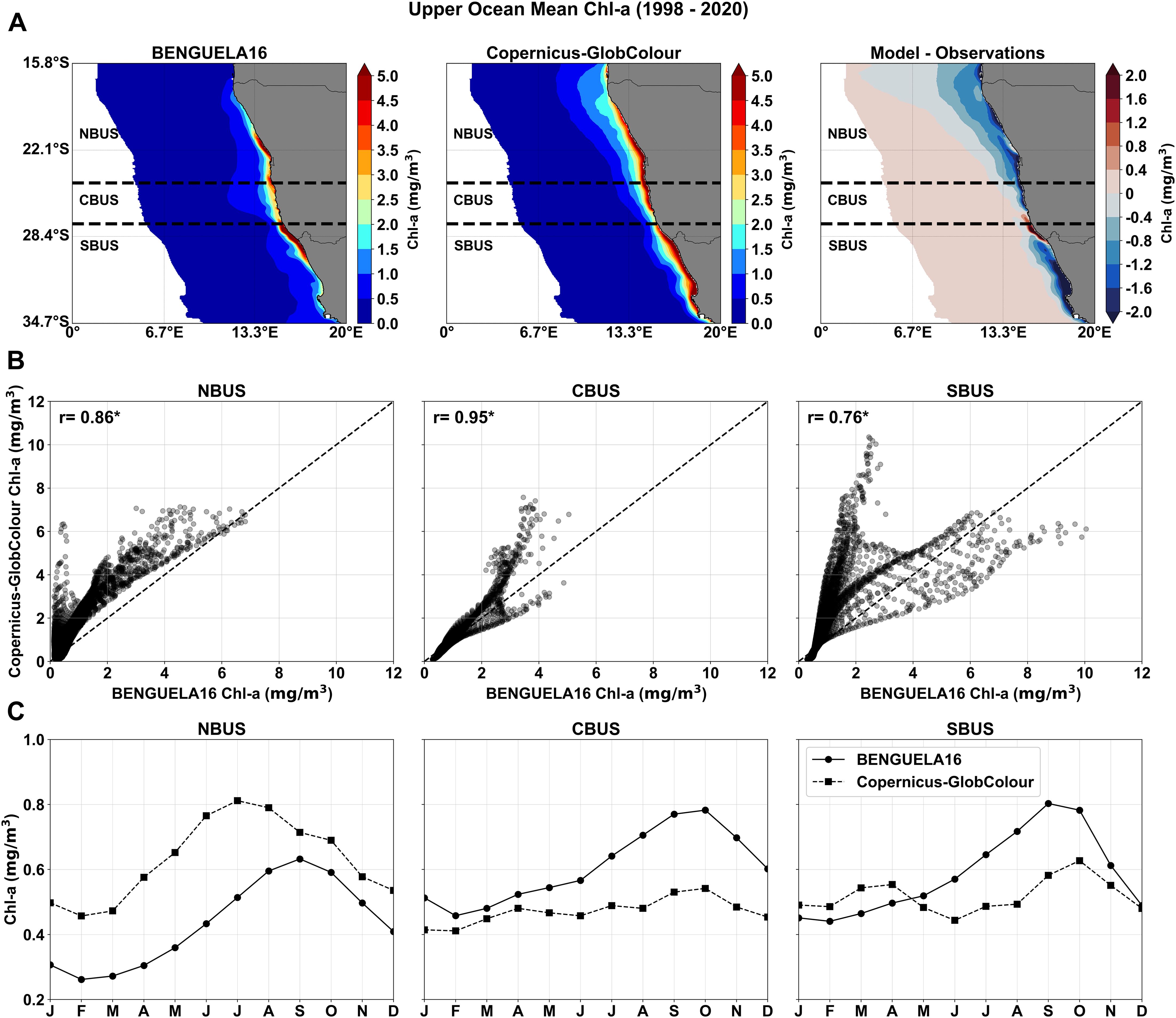
Figure 11. Comparison of the 1998–2020 climatological fields of the upper ocean Chl-a concentrations from BENGUELA16 simulations and Copernicus-GlobColour satellite data (CMEMS, 2023) for an area extending ~1000 km offshore from the Benguela region coastline. (A) Spatial distribution of the upper ocean Chl-a from BENGUELA16 (left) and Copernicus-GlobColour (center) data, along with their difference (right). Dashed horizontal lines indicate the BUS subregions: NBUS (Northern Benguela), CBUS (Central Benguela), and SBUS (Southern Benguela). (B) Scatter plot of simulated vs observed Chl-a concentrations at each model’s grid point within the selected coastal band for the three subregions. The dashed line indicates the ideal fit and the Pearson’s correlation coefficient (r) is marked with an asterisk if statistically significant (p < 0.05). (C) Annual cycle of monthly Chl-a mean values over each subregion as obtained from BENGUELA16 and Copernicus-GlobColour data.

The comparison of spatially and monthly averaged surface Chl-a between BFM and Copernicus-GlobColour data (Figure 11C) shows the model effectively reproduces the annual cycle across all three subregions. In the central and southern Benguela, the Chl-a peak (August–October) matches observations, whereas in the northern Benguela, the peak is delayed relative to satellite data (June–August). While the seasonal cycle is well captured, biases persist: BENGUELA16 underestimates Chl-a by approximately 0.24 mg/m³ (January–August) in the NBUS and overestimates it by ~0.25 mg/m³ in the central and southern subregions.

A comparison between simulated monthly mean Chl-a profiles from BENGUELA16 and multiprofile observations from BGC-ARGO over the SBUS open waters during the period from December 2014 to September 2018 is illustrated in Figure 12. Overall, the model satisfactorily reproduces the vertical distribution patterns of Chl-a, with data showing a typical biologically active layer extending from the surface to approximately 100 meters. Furthermore, the model captures the observed seasonality to a large extent, with deeper and lower Chl-a concentrations during the austral winter and the occurrence of the subsurface maxima during the austral summer. However, the model systematically underestimates Chl-a concentrations, particularly in upper layers, where BGC-ARGO observations frequently exceed 0.60 mg/m³, whereas BENGUELA16 simulations mostly remain below 0.40 mg/m³.

Figure 12

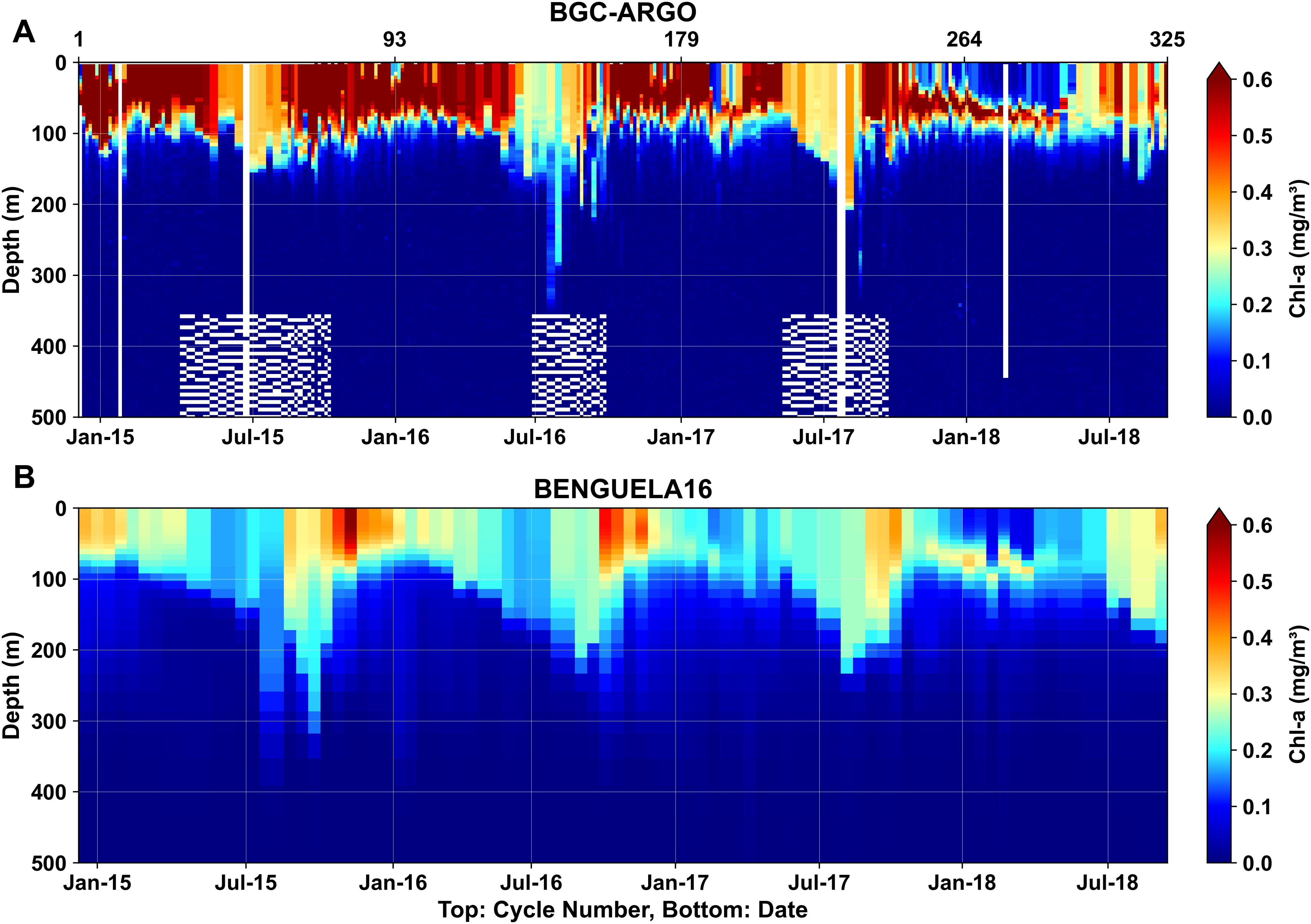
Figure 12. Hovmöller comparison of Chl-a multi-profiles from (A) the BGC-ARGO float number 6901582 (Wong et al., 2020) and (B) the BENGUELA16 outputs. BENGUELA16 data correspond to the nearest grid cell and sampling date of each BGC-ARGO sample. White blanks indicate missing data. The profiles span from December 2014 to September 2018, with their locations illustrated in Figure 3A. The top x-axis denotes the profile number, the bottom x-axis represents the date, and the y-axis indicates depth (m).

3.3 Long-term trends

The long-term trends of sea surface temperature and upper ocean Chl-a concentrations (Figure 13) have been estimated from the simulated data over the BENGUELA16 domain and the satellite-based datasets ESA-CCI and Copernicus-GlobColour (see Section 2.3 for details). Data were averaged longitudinally over a 1° band from the coastline to retain the upwelling activity zone and scaled to express decadal rates of change. We used linear least-squares regression to obtain the trends at each grid point over the latitudinal range. For the trend analysis, only statistically significant trends with p-values < 0.05 are considered.

Figure 13

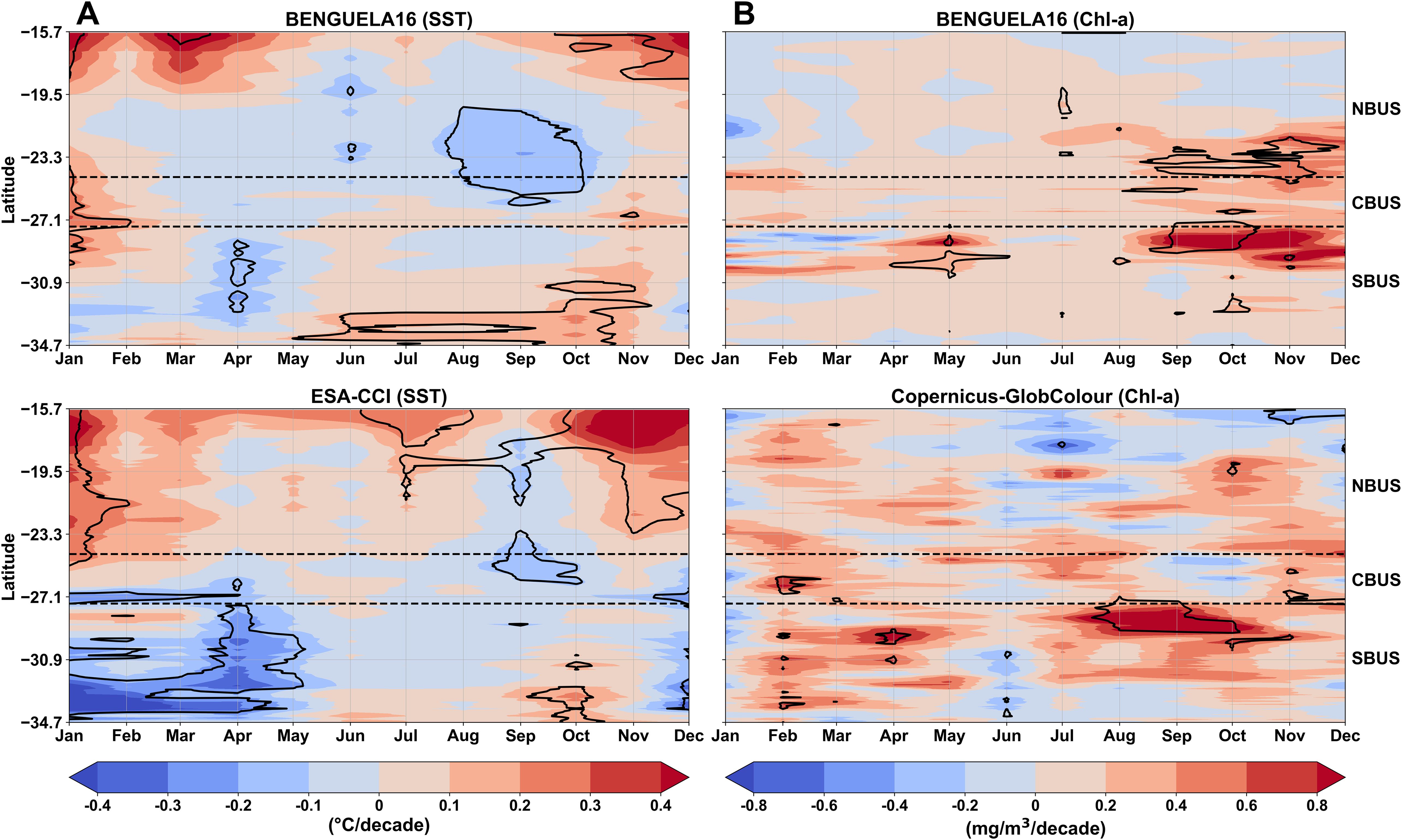
Figure 13. Long-term trends in sea surface temperature (SST; °C/decade) (A), and the upper ocean Chl-a concentrations (mg/m³ per decade) (B), computed from the BENGUELA16 simulated data (top panels) and satellite-based observations of ESA-CCI (1982–2020) and Copernicus-GlobColour (1998–2020) datasets (bottom panels). Data were longitudinally averaged over a ~100 km band from the coastline and span the latitudinal range of 15.7°S to 34.7°S. Black contour lines represent statistically significant trends (p < 0.05). Horizontal dashed lines indicate the boundaries of the three subregions: Northern Benguela (NBUS), Central Benguela (CBUS), and Southern Benguela (SBUS).

In general, the trends derived from the BENGUELA16 SST data show strong coherence with those from the ESA-CCI dataset (Figure 13A). A cooling trend of -0.12 °C per decade is identified between 20°S and 26°S, with the model indicating a broader seasonal span from August to October. This negative trend extends into the central Benguela subregion. However, in this area, the two datasets show contrasting signs in the trends during the austral summer. Both datasets indicate cooling across the southern subregion during the austral summer, though ESA-CCI reveals a more intense and seasonally extensive cooling, with trends reaching up to -0.64 °C per decade, compared to a maximum of -0.24 °C per decade in the model.

The BENGUELA16 simulation also captures three statistically significant warming patterns: i) in the Angola-Benguela Frontal Zone (ABFZ, 15.7°S–18.7°S) during late austral spring and summer (October to January), with values up to 0.40 °C per decade; ii) in central Benguela (24.5°S–27.5°S), a weaker warming of about 0.25 °C per decade is observed in January; iii) in southern Benguela (30.7°S–34.7°S), a more modest warming trend of 0.15 °C per decade extends from austral autumn through spring (May to November).

For upper ocean Chl-a trends, the comparison between BENGUELA16 and CopernicusGlobColour reveals several similarities, particularly in regions with positive trends (Figure 13B). Both datasets show statistically significant increases in Chl-a exceeding 0.80 mg/m³ per decade during late austral winter and spring (August to October), especially over southern Benguela (27°S–29°S). BENGUELA16 also shows a positive trend at 29°S during austral autumn, although with lower intensity (0.20–0.40 mg/m³) compared to satellite estimates (0.60–0.80 mg/m³). Differences between the datasets become more pronounced in the central and southern Benguela during austral summer (February), while the positive trend emerging in April in satellite data also appears in the model, though delayed by one month. Additionally, Copernicus-GlobColour shows a small but statistically significant negative trend over the ABFZ during austral summer, which is not captured by the model.

Overall, the BENGUELA16 regional model shows good skill in capturing the spatio-temporal patterns and intensity of SST trends, and to a lower extent, those of Chl-a concentrations.

4 Discussion

4.1 Limitations of the BUS modeling system

As illustrated in Figure 4, the global domain physical component exhibits systematic biases for both SST and SSS in correspondence with the western boundary currents, namely the Gulf Stream and the Kuroshio Current—similar to findings from previous modeling studies (Bryan et al., 2007; He et al., 2014; Renault et al., 2019; Liu et al., 2023). As shown by Iovino et al. (2023), the model’s horizontal resolution poses certain limitations on its ability to reproduce the spatial variability of these highly dynamic systems. Along with grid resolution, certain model parameterizations also contribute to the emergence of such biases. Kamenkovich et al. (2000) demonstrated that horizontal viscosity plays a critical role in shaping the dynamics of western boundary currents. Furthermore, Renault et al. (2019) showed that incorporating air-sea feedbacks, particularly through the eddy killing mechanism, can help mitigate persistent biases in simulations of western boundary currents. Although the model is forced with high-frequency GloFAS runoff data, local positive and negative surface salinity anomalies remain evident along coastal areas. This is likely related to the use of zero-salinity inputs, which may underrepresent the real runoff characteristics and would benefit from the imposition of ad-hoc salinity values at river outlets.

The physical component of the BENGUELA16 configuration is characterized by positive salinity biases along its southern boundary (Figures 6D–F; Supplementary Figure S4), indicating a deficiency in reproducing freshwater masses entering the BUS from the Southern Ocean. These waters typically feed into the South Atlantic gyre and introduce fresher water along the South African coast (Beal et al., 2011). This bias may also be linked to limitations in representing the northward displacement of the South Atlantic Subtropical Front, which influences both the influx of low-salinity water and the zonal extent of the Agulhas Retroflection.

Marine biogeochemical variables show varying levels of agreement with the selected observational datasets (see Section 3.2.2). The comparison of NO₃^- and PO₄^3- with both gridded and in-situ data indicates that biases mainly affect the surface and subsurface layers. This discrepancy can be attributed to an intense biological consumption in the model, resulting in lower nutrient concentrations. Additionally, the offshore advection of newly upwelled waters may rapidly transport nutrients away from the coast, reducing their residence time and limiting phytoplankton growth. This mechanism is also linked to the slight overestimation of near-surface current speeds compared to OSCAR data, especially over the narrow coastal shelf (Figures 6G–I).

Dissolved oxygen biases along the western and southern boundaries of the regional domain, particularly between 500 and 1000 m depth (Supplementary Figure S5), are primarily attributed to lower accuracy in the boundary condition data used to prescribe oxygen influxes from the Southern Ocean. The comparison with glider measurements in the northern Benguela subregion (Figure 10) indicates that simulated oxygen profiles generally match observations in the upper and deeper layers, but the model underestimates concentrations by about 30 mmol O₂/m³ at intermediate depths around 200 m. This difference likely results from a combination of unrealistic oxygen levels in the Southern Atlantic Central Water entering the region (see Mohrholz et al., 2008; Schmidt and Eggert, 2016) and enhanced oxygen consumption due to heterotrophic bacterial remineralization of organic matter.

Coastal Chl-a values within the first 100 km of the upwelling zone are underestimated, while concentrations in the open ocean—especially in the central and southern regions, are slightly overestimated. This is more evident in the punctual comparison of simulated and satellite-derived Chl-a fields (Figure 11B). In southern Benguela, the pattern of over- and underestimated values near the coast deviates notably from the ideal fit, while open ocean data are in better agreement. Nevertheless, the spatially averaged annual cycle (Figure 11C) shows that the model adequately captures the seasonal variability of algal blooms, especially in the NBUS, where Chl-a concentrations peak in August, December, and April, as previously reported by Louw et al. (2016).

However, comparing model outputs with satellite data in optically complex coastal waters remains challenging. In fact, satellite measurements of spectral reflectance can be influenced by factors unrelated to phytoplankton abundance, such as the presence of colored dissolved organic matter (Siegel et al., 2005; Aurin and Dierssen, 2012) and suspended particulates that alter light attenuation (Chauhan et al., 2002; Gohin, 2011; Theenathayalan et al., 2022). As a result, satellite retrieval algorithms are subject to greater uncertainty in these regions and may sometimes overestimate Chl-a concentrations (Coelho et al., 2017; Poddar et al., 2019).

4.2 Strengths of the BUS modeling system

The comparison of long-term mean state physical fields in the global and regional domains of the BUS modeling system shows that biases are generally modest, with a good reproduction of climatological physical patterns. In the validation of the ORCA025L75 global domain (Figure 4), temperature and salinity showed realistic spatial patterns, and a rather low bias was obtained for near-surface current speed fields. The global configuration also provided a reliable representation of the seawater temperature and salinity fields in the subsurface ocean at most of the selected depth levels (Figure 5).

The reproduction of physical fields in the BENGUELA16 regional domain was remarkable, as in the comparison with satellite observations (Figure 6) and ARMOR3D analysis data at different depths (Figure 7), where the obtained biases were comparable and in some cases lower than previous similar modeling applications (Veitch et al., 2009; Gutknecht et al., 2013). The regional configuration effectively captures the horizontal and vertical spatial patterns of seawater physical parameters as determined by the Benguela coastal upwelling dynamics. The low SST values obtained along the Namibian shelf (Figure 6A) indicate the ascent of cold waters from deeper layers, with an extension of the coastal upwelling plume comparable to that observed by satellite surveys. Along the vertical, the simulated upward tilting of isolines with the consequent outcropping of deeper water compares well with ARMOR3D analysis fields (Figure 8), particularly over the narrow coastal shelf despite some minor underestimations. Near-surface current speeds produced by the Benguela regional configuration are also largely coherent with those available from the OSCAR Analysis (Figures 6G–I) and with the circulation patterns described in previous oceanographic studies (Stramma and Peterson, 1989; Lutjeharms, 2007; Beal et al., 2011; Tim et al., 2018; Majumder and Schmid, 2018). The model clearly shows the northwestward flow of the Benguela Current around 27°S that is fuelled by the Southern Atlantic and Indian Oceans via the South Atlantic Current. Furthermore, the BENGUELA16 physical component consistently simulates the Agulhas retroflection at about 16°E, which generates the Agulhas Return Current directed toward the Indian Ocean subtropical gyre and the Agulhas leakage’s mesoscale eddies propagating into the South Atlantic gyre (Reason et al., 2003).

The long-term mean fields of NO₃^- and PO₄^3- exhibited reasonably good skills at the different vertical layers (Figure 7), as the BENGUELA16 data don’t significantly deviate from the mean state representation of the CARS climatology. Conversely, the evaluation against in-situ data from the JC032 and Afr258 cruises showed a better agreement (Figure 9). In particular, the comparison of longitudinal sections with JC032 data shows a good representation of nutrient concentration isoline deformation caused by the coastal upwelling (Figures 9C, D). Dissolved oxygen long-term mean fields of BENGUELA16 showed to be consistent with CARS climatology, particularly within the biologically active upper layers (0–200 m), while oxygen levels were underestimated at depths over the central and northern Benguela shelf (Supplementary Figure S5). However, the model successfully captured key DO dynamics, including the distribution of hypoxic waters (< 60 mmol O₂/m³), particularly in the northern Benguela, where the Southern Atlantic Central Water transports oxygen-depleted waters via the poleward undercurrent (Monteiro and van der Plas, 2006; Mohrholz et al., 2008; Lass and Mohrholz, 2008). The validation of simulated upper-ocean Chl-a concentrations against satellite data shows how the model is capable of capturing the upwelling-driven response of phytoplankton, as the onshore-offshore Chl-a gradient observed in Copernicus-GlobColour data is well represented (Figure 11A), with additional skills in the reproduction of the whole seasonal cycle (Figure 11C). Moreover, the comparison with Chl-a vertical profiles collected by the ARGO-BGC float indicated the satisfactory skills of the model in replicating the depth and structure of the vertical Chl-a distribution over space and time.

Overall, the coupled modeling system effectively captures the key physical and biogeochemical dynamics of the Benguela Upwelling System, and it may be further exploited to support a range of applications aimed at monitoring system dynamics. From a physical perspective, different indices can be implemented to assess the variability of upwelling intensity by exploiting either SST changes along the Namibian shelf (Chen et al., 2012; Santos et al., 2012) or the simulated current velocities to estimate offshore Ekman transport across the different subregions (Veitch et al., 2010). Moreover, the combined use of physical and biogeochemical quantities enables the application of the Biologically Effective Upwelling Transport Index (BEUTI; Jacox et al., 2018), which evaluates nitrate flux into the photic zone. The good performance of the modeling system in representing dissolved oxygen across various depths also makes it well-suited for studying long-term trends in minimum oxygen zones, particularly under intensified upwelling conditions (Bakun et al., 2015). Finally, model outcomes could be further utilized to monitor the evolution of the Benguela marine ecosystem and assess potential impacts on productivity, habitat quality, and fisheries potential, helping to identify oceanographic shifts that support informed, climate-resilient management of coastal areas (Chang et al., 2023; Lamont et al., 2019).

4.3 Long-term trends and their implications for upwelling intensification

Sea surface temperature is widely recognized as a reliable proxy for assessing both temporal and spatial variability in upwelling intensity (Gutierrez-Guerra et al., 2024), due to its theoretical connection to the ascent of deep, cold water to the surface layer. The model outcomes reveal a significant cooling trend in both the northern and southern Benguela subregions, during their respective upwelling seasons. In the northern Benguela, a cooling trend is evident during late austral winter and austral spring (Figure 13A), which is the primary upwelling season for this subregion (Shannon, 1985; Hagen et al., 2001; Tim et al., 2015). Similarly, in southern Benguela, the strongest cooling trend occurs during its upwelling season, namely from December to May (Rixen et al., 2021; Rouault and Tomety, 2022).

When comparing the simulated SST seasonal trends with those from ESA-CCI satellite data, the model demonstrates good skill in detecting cooling patterns in northern and southern subregions, particularly during upwelling seasons. However, some discrepancies in the spatial and temporal distribution and intensity of these trends emerged, particularly in the ABFZ and within southern Benguela. These discrepancies may be explained by the model having produced a weaker water inflow from the Angola Current resulting in a lower extent of the warming trend in the NBUS, while the simulated upwelling signal in the SBUS is weakened by a stronger Agulhas warm-water intrusion during the austral spring and autumn.

Nevertheless, the model’s outcomes align with previous observational studies. For example, Tomety et al. (2024) identified a significant cooling trend in satellite-derived SST data in the northern Benguela subregion (23°S–25°S) during austral spring between 1982 and 2015, with a cooling rate of -0.10 to -0.20 °C per decade, similar to our results (Figure 13A).

A warming trend in the ABFZ latitudes (16°S) is consistent with findings from previous studies. Tomety et al. (2024) reported a significant warming trend during austral summer (DJF), in addition, Monteiro and van der Plas (2006) documented a warming trend in SST over the ABFZ, with values exceeding 0.60 °C per decade from 1982 to 2005. This warming trend may be linked to latitudinal shifts in its position, likely driven by the southward intrusion of the warmer Angola Current into the cooler Benguela Upwelling Zone. Vizy et al. (2018) reported a southward latitudinal shift of 0.05° – 0.55° per decade between 1980 and 2014. The ABFZ follows a pronounced semi-annual cycle, peaking between November and December (Koseki et al., 2019), which aligns with our detected warming trends in the region during these months. Variability in its position and intensity can significantly impact the coastal ecosystem, as warm and nutrient-poor intrusions may alter biological communities (Huenerlage and Buchholz, 2013).

Several studies converged on the coastal SST cooling along the BUS at the annual scale, attributing this primarily to upwelling intensification (Santos et al., 2012; Polonsky and Serebrennikov, 2021; Gutierrez-Guerra et al., 2024). Polonsky and Serebrennikov (2021) noted a cooling tendency in the Benguela coastaloceanic thermal gradient, accompanied by an intensification of the Ekman transport. Gutierrez-Guerra et al. (2024) assessed changes across all Eastern Boundary Upwelling Systems, identifying a negative trend (-0.23°C per decade) in the BUS coastal waters. The cooling trends simulated by the BENGUELA16 physical component, which moderately coincide with satellite observations during upwelling seasons, are much more likely pointing to an upwelling intensification.

The simulated surface Chl-a trends (Figure 13B) show statistically significant positive trends over a few locations, indicating an overall increase in upper Chl-a concentrations over the studied period (1998–2020). In particular, the comparison with Copernicus-GlobColour data showed that the model is able to detect the main positive trend in southern Benguela. However, discrepancies exist, such as the simulated positive trend over the northern Benguela during the austral spring, which is not evident in satellite observations. These may be related to inherent limitations of satellite-derived Chl-a data (see Section 4.1) or potential shortcomings in the model, indicating further required improvement in the simulation of Chl-a levels.

The model-derived positive Chl-a trends, which are potentially linked to upwelling intensification, are also consistent with previous studies. Gregg et al. (2005) noted a positive Chl-a trend along the Namibian-Angolan coast between 1998 and 2003. Verheye (2000) documented an increase in surface Chl-a concentrations between March and June in St. Helena Bay (32°S). Bordbar et al. (2021) observed a significant correlation between the spatial patterns of Chl-a and upwelling intensity from 2008 to 2018 in the whole BUS region. Similarly, Chen et al. (2012) reported a strong positive correlation between upwelling intensity and Chl-a across latitudes from 23°S to 34°S during the 2003–2008 period.

The simulated trends reveal an inverse proportionality between Chl-a and SST trends. The positive Chl-a trends in northern Benguela correspond to the cooling trend of SST found at the same latitudes and seasons. In northern Benguela, the positive Chl-a trend slightly aligns with the detected cooling, though with a one-month temporal lag (Figures 13A,B). This relationship supports the linkage between upwelling intensification, surface water cooling, and increasing activity of primary producers (García-Reyes et al., 2015). However, an increase in primary producers’ activity does not always directly correlate with stronger upwelling. Enhanced upwelling typically draws nutrient-rich water into the mixed layer, but our trend comparisons suggest this conceptual framework may not apply across all the Benguela subregions.

A stronger cooling trend may occur without a corresponding positive Chl-a trend, as observed in southern Benguela during austral summer and autumn. In the proposed modeling framework, this could be due to intensified upwelling activity enhancing dilution, further limiting Chl-a accumulation, or to an already saturated phytoplankton growth regulated by top-down control. While upwelling generally stimulates phytoplankton growth by transporting nutrient-rich water to the surface (Bakun et al., 2015), other factors—including the chemical composition of the upwelled water, can significantly influence primary production (Rykaczewski and Dunne, 2010; Bograd et al., 2015). Jacox et al. (2018) noted that subsurface nutrient concentrations may vary independently of local upwelling vertical transport. Flynn et al. (2020) reported that in southern Benguela, primary production is not exclusively tied to upwelling signals, as high nutrient fluxes are regenerated over the continental shelf (i.e., nutrient trapping), providing variability in primary producers independent of upwelling-derived nutrients.

Finally, intensified upwelling in the BUS may boost primary producers and consumers in surface waters but also increase organic export, enhancing microbial respiration that depletes O₂ and raises CO₂ (Gruber, 2011). This can induce hypoxic conditions over the continental shelf, threatening marine life (Grantham et al., 2004; Chan et al., 2008). The exposure of the upper ocean ecosystem to more acidic conditions during the upwelling events may have detrimental effects on marine biota (Lluch-Cota et al., 2014; Bakun et al., 2015). Moreover, changes in upwelling timing can disrupt predator-prey dynamics and affect productivity in upwelling regions (Schwing et al., 2006).

5 Conclusions

This study demonstrates the effectiveness of a high-resolution coupled physical-biogeochemical modeling system in capturing the dynamics of the Benguela Upwelling System over long-term timescales. The regional BENGUELA16 configuration successfully reproduces key physical and biogeochemical features, including mesoscale circulation patterns, coastal upwelling and its role in vertical nutrient transport, low-oxygen concentrations in shelf waters, and the characteristic onshore–offshore Chl-a gradient.

The analysis of long-term sea surface temperature trends revealed significant cooling (-0.20 °C per decade) during the upwelling seasons in the northern and southern Benguela regions, suggesting a steady intensification of upwelling dynamics over the past four decades. However, this trend is not reflected in the companion analysis of upper ocean Chl-a, neither in the model nor in the satellite data. This discrepancy warrants further investigation to better understand the environmental factors that may be counteracting the expected biological response to intensified upwelling.

Beyond validation, the modeling system provides a sound basis for future applications, such as the development of upwelling indices to monitor changes in marine ecosystem productivity and potential impacts on upper trophic levels—for example, by feeding information into fisheries models. Thanks to its spatial resolution and extended temporal coverage, the coupled model outputs may also be used to examine the evolution of oxygen minimum zones in the northern subregion and assess their evolution under warming climate conditions. To a broader extent, the insights produced in this work could be exploited to develop regional observational strategies and inform resource management plans in one of the world’s most productive eastern boundary upwelling systems.

Data availability statement

The raw data supporting the conclusions of this article will be made available by the authors, without undue reservation.

Author contributions

AS: Data curation, Visualization, Methodology, Conceptualization, Writing – review & editing, Writing – original draft, Validation. TL: Writing – review & editing, Validation, Data curation, Methodology, Conceptualization. MB: Writing – review & editing, Conceptualization. MZ: Writing – review & editing, Conceptualization.

Funding

The author(s) declare that financial support was received for the research and/or publication of this article. AS, TL, and MB acknowledge funding from the European Union’s Horizon 2020 research and innovation programmes (grant agreement no. 862923) (AtlantECO).

Acknowledgments

Thanks to the “CMCC Foundation - Euro-Mediterranean Center on Climate Change, Bologna, Italy” for providing access to the High-performance computing (ZEUS), which has been instrumental in facilitating the computational aspects of this research.

Conflict of interest

The authors declare that the research was conducted in the absence of any commercial or financial relationships that could be construed as a potential conflict of interest.

The author(s) declared that they were an editorial board member of Frontiers, at the time of submission. This had no impact on the peer review process and the final decision.

Generative AI statement

The author(s) declare that no Generative AI was used in the creation of this manuscript.

Publisher’s note

All claims expressed in this article are solely those of the authors and do not necessarily represent those of their affiliated organizations, or those of the publisher, the editors and the reviewers. Any product that may be evaluated in this article, or claim that may be made by its manufacturer, is not guaranteed or endorsed by the publisher.

Supplementary material

The Supplementary Material for this article can be found online at: https://www.frontiersin.org/articles/10.3389/fmars.2025.1601284/full#supplementary-material

Supplementary Figure 1 | Comparison of sea surface temperature (SST) seasonal climatologies between NEMO (left) and ESA-CCI (Merchant et al., 2019) (centre) and their difference (right).

Supplementary Figure 2 | Comparison of sea surface salinity (SSS) seasonal climatologies between NEMO (left) and ESA-CCI (Boutin et al., 2021) (centre) and their difference (right).

Supplementary Figure 3 | SST seasonal climatology comparison from NEMO (left) and ESA-CCI (Merchant et al., 2019) (centre) and their difference (right) over the BENGUELA16 domain.

Supplementary Figure 4 | Seasonal climatology comparison between NEMO (left) and ESA-CCI (Boutin et al., 2021) (centre) SSS and their difference (right) over the BENGUELA16 domain.

Supplementary Figure 5 | Comparison of BENGUELA16 (left) and CARS (CARS, 2009) (centre) dissolved oxygen annual climatology (1980 - 2020) and their difference (right) at different vertical depths (0, 50, 100, 500, and 1000 meters).

References

Alfieri L., Burek P., Dutra E., Krzeminski B., Muraro D., Thielen J., et al. (2013). Glofas–global ensemble streamflow forecasting and flood early warning. Hydrology Earth System Sci. 17, 1161–1175. doi: 10.5194/hess-17-1161-2013

Crossref Full Text | Google Scholar

Aumont O., Éthé C., Lovato T., Mouchet A., Nurser G., Palmiéri J., et al. (2019). Tracers in Ocean Paradigm (TOP)–The NEMO Tracers engine. France: Notes du Pôle de modélisation de l'Institut Pierre-Simon Laplace (IPSL) doi: 10.5281/zenodo.1471700

Crossref Full Text | Google Scholar

Aurin D. A. and Dierssen H. M. (2012). Advantages and limitations of ocean color remote sensing in cdom-dominated, mineral-rich coastal and estuarine waters. Remote Sens. Environ. 125, 181–197. doi: 10.1016/j.rse.2012.07.001

Crossref Full Text | Google Scholar

Bakun A. (1990). Global climate change and intensification of coastal ocean upwelling. Science 247, 198–201. doi: 10.1126/science.247.4939.198

PubMed Abstract | Crossref Full Text | Google Scholar

Bakun A., Black B. A., Bograd S. J., Garcia-Reyes M., Miller A. J., Rykaczewski R. R., et al. (2015). Anticipated effects of climate change on coastal upwelling ecosystems. Curr. Climate Change Rep. 1, 85–93. doi: 10.1007/s40641-015-0008-4

Crossref Full Text | Google Scholar

Beal L. M., De Ruijter W. P., Biastoch A., and Zahn R. (2011). On the role of the agulhas system in ocean circulation and climate. Nature 472, 429–436. doi: 10.1038/nature09983

PubMed Abstract | Crossref Full Text | Google Scholar

Biastoch A., Rühs S., Ivanciu I., Schwarzkopf F. U., Veitch J., Reason C., et al. (2024). “The agulhas current system as an important driver for oceanic and terrestrial climate,” in Sustainability of Southern African Ecosystems Under Global Change: Science for Management and Policy Interventions (Cham, Switzerland: Springer), 191–220. doi: 10.1007/978-3-031-10948-5_8

Crossref Full Text | Google Scholar

Blanke B. and Delecluse P. (1993). Variability of the tropical atlantic ocean simulated by a general circulation model with two different mixed-layer physics. J. Phys. Oceanography 23, 1363–1388. doi: 10.1175/1520-0485(1993)023<1363:VOTTAO>2.0.CO;2

Crossref Full Text | Google Scholar

Bograd S. J., Buil M. P., Di Lorenzo E., Castro C. G., Schroeder I. D., Goericke R., et al. (2015). Changes in source waters to the southern california bight. Deep Sea Res. Part II: Topical Stud. Oceanography 112, 42–52. doi: 10.1016/j.dsr2.2014.04.009

Crossref Full Text | Google Scholar

Bordbar M. H., Mohrholz V., and Schmidt M. (2021). The relation of wind-driven coastal and offshore upwelling in the benguela upwelling system. J. Phys. Oceanography 51, 3117–3133. doi: 10.1175/JPO-D-20-0297.1

Crossref Full Text | Google Scholar

Boutin J., Reul N., Köhler J., Martin A., Catany R., Guimbard S., et al. (2021). Satellite-based sea surface salinity designed for ocean and climate studies. J. Geophysical Research: Oceans 126, e2021JC017676. doi: 10.1029/2021JC017676

Crossref Full Text | Google Scholar

Brandt P., Bordbar M. H., Coelho P., Koungue R. A. I., Körner M., Lamont T., et al. (2024). “Physical drivers of southwest african coastal upwelling and its response to climate variability and change,” in Sustainability of Southern African Ecosystems under Global Change: Science for Management and Policy Interventions (Cham, Switzerland: Springer), 221–257. doi: 10.1007/978-3-031-10948-5_9

Crossref Full Text | Google Scholar

Brodeau L., Barnier B., Gulev S. K., and Woods C. (2017). Climatologically significant effects of some approximations in the bulk parameterizations of turbulent air–sea fluxes. J. Phys. Oceanography 47, 5–28. doi: 10.1175/JPO-D-16-0169.1

Crossref Full Text | Google Scholar

Bryan F. O., Hecht M. W., and Smith R. D. (2007). Resolution convergence and sensitivity studies with north atlantic circulation models. part i: The western boundary current system. Ocean Model. 16, 141–159. doi: 10.1016/j.ocemod.2006.08.005

Crossref Full Text | Google Scholar

Carr M.-E. (2001). Estimation of potential productivity in eastern boundary currents using remote sensing. Deep Sea Res. Part II: Topical Stud. Oceanography 49, 59–80. doi: 10.1016/S0967-0645(01)00094-7

Crossref Full Text | Google Scholar

CARS (2009). Cars 2009 dataset. Available online at: http://www.marine.csiro.au/~dunn/cars2009/ (Accessed September 15, 2023).

Google Scholar

Chan F., Barth J., Lubchenco J., Kirincich A., Weeks H., Peterson W. T., et al. (2008). Emergence of anoxia in the california current large marine ecosystem. Science 319, 920–920. doi: 10.1126/science.1149016

PubMed Abstract | Crossref Full Text | Google Scholar

Chang P., Xu G., Kurian J., Small R. J., Danabasoglu G., Yeager S., et al. (2023). Uncertain future of sustainable fisheries environment in eastern boundary upwelling zones under climate change. Commun. Earth Environ. 4, 19. doi: 10.1038/s43247-023-00681-0

Crossref Full Text | Google Scholar

Chauhan P., Mohan M., Nayak S., and Navalgund R. (2002). Comparison of ocean color chlorophyll algorithms for irs-p4 ocm sensor using in-situ data. J. Indian Soc. Remote Sens. 30, 87–94. doi: 10.1007/BF02989980

Crossref Full Text | Google Scholar

Chen Z., Yan X.-H., Jo Y.-H., Jiang L., and Jiang Y. (2012). A study of benguela upwelling system using different upwelling indices derived from remotely sensed data. Continental shelf Res. 45, 27–33. doi: 10.1016/j.csr.2012.05.013

Crossref Full Text | Google Scholar

CMEMS (2022). Multi observation global ocean 3d temperature salinity height geostrophic current and mld. E.U. Copernicus Marine Service Information (CMEMS) (Marine Data Store (MDS). doi: 10.48670/moi-00052

Crossref Full Text | Google Scholar

CMEMS (2023). Global ocean colour (copernicus-globcolour), bio-geo-chemical, l4 (monthly and interpolated) from satellite observations (1997-ongoing) (Marine Data Store (MDS). doi: 10.48670/moi-00281

Crossref Full Text | Google Scholar

Coelho C., Heim B., Foerster S., Brosinsky A., and De Araújo J. C. (2017). In situ and satellite observation of cdom and chlorophyll-a dynamics in small water surface reservoirs in the Brazilian semiarid region. Water 9, 913. doi: 10.3390/w9120913

Crossref Full Text | Google Scholar

Cury P. and Roy C. (1989). Optimal environmental window and pelagic fish recruitment success in upwelling areas. Can. J. Fisheries Aquat. Sci. 46, 670–680. doi: 10.1139/f89-08

Crossref Full Text | Google Scholar

Debreu L., Marchesiello P., Penven P., and Cambon G. (2012). Two-way nesting in splitexplicit ocean models: Algorithms, implementation and validation. Ocean Model. 49, 1–21. doi: 10.1016/j.ocemod.2012.03.003

Crossref Full Text | Google Scholar

ESR (2009). Oscar third degree resolution ocean surface currents. Ver. 1 (California, USA: NASA Physical Oceanography Distributed Active Archive Center (PO.DAAC)). doi: 10.5067/OSCAR-03D01

Crossref Full Text | Google Scholar

Flohr A., van der Plas A., Emeis K.-C., Mohrholz V., and Rixen T. (2014). Spatio-temporal patterns of c: N: P ratios in the northern benguela upwelling system. Biogeosciences 11, 885–897. doi: 10.5194/bg-11-885-2014

Crossref Full Text | Google Scholar

Flynn R., Granger J., Veitch J., Siedlecki S., Burger J., Pillay K., et al. (2020). On-shelf nutrient trapping enhances the fertility of the southern benguela upwelling system. J. Geophysical Research: Oceans 125, e2019JC015948. doi: 10.1029/2019JC015948

Crossref Full Text | Google Scholar

Garcia H., Weathers K., Paver C., Smolyar I., Boyer T., Locarnini M., et al. (2019a). World ocean atlas 2018. Vol. 4: Dissolved inorganic nutrients (phosphate, nitrate and nitrate+ nitrite, silicate) (USA: National Oceanic and Atmospheric Administration). Available online at: https://www.ncei.noaa.gov/data/oceans/woa/WOA18 (Accessed November 15, 2024).

Google Scholar

Garcia H., Weathers K., Paver C., Smolyar I., Boyer T., Locarnini M., et al. (2019b). World Ocean Atlas 2018, Volume 3: Dissolved Oxygen, Apparent Oxygen Utilization, and Dissolved Oxygen Saturation (USA: National Oceanic and Atmospheric Administration). Available online at: https://www.ncei.noaa.gov/data/oceans/woa/WOA18 (Accessed November 15, 2024).

Google Scholar

García-Reyes M., Sydeman W. J., Schoeman D. S., Rykaczewski R. R., Black B. A., Smit A. J., et al. (2015). Under pressure: Climate change, upwelling, and eastern boundary upwelling ecosystems. Front. Mar. Sci. 2. doi: 10.3389/fmars.2015.00109

Crossref Full Text | Google Scholar

GEBCO Compilation Group (2021). GEBCO 2021 Grid. doi: 10.5285/c6612cbe-50b3-0cff-e053-6c86abc09f8f

Crossref Full Text | Google Scholar

Gohin F. (2011). Annual cycles of chlorophyll-a, non-algal suspended particulate matter, and turbidity observed from space and in-situ in coastal waters. Ocean Sci. 7, 705–732. doi: 10.5194/os-7-705-2011

Crossref Full Text | Google Scholar

Goutorbe B., Poort J., Lucazeau F., and Raillard S. (2011). Global heat flow trends resolved from multiple geological and geophysical proxies. Geophysical J. Int. 187, 1405–1419. doi: 10.1111/j.1365-246X.2011.05228.x

Crossref Full Text | Google Scholar

Grantham B. A., Chan F., Nielsen K. J., Fox D. S., Barth J. A., Huyer A., et al. (2004). Upwellingdriven nearshore hypoxia signals ecosystem and oceanographic changes in the northeast pacific. Nature 429, 749–754. doi: 10.1038/nature02605

PubMed Abstract | Crossref Full Text | Google Scholar

Gregg W. W., Casey N. W., and McClain C. R. (2005). Recent trends in global ocean chlorophyll. Geophysical Res. Lett. 32. doi: 10.1029/2004GL021808

Crossref Full Text | Google Scholar

Gruber N. (2011). Warming up, turning sour, losing breath: ocean biogeochemistry under global change. Philos. Trans. R. Soc. A: Mathematical Phys. Eng. Sci. 369, 1980–1996. doi: 10.1098/rsta.2011.0003

PubMed Abstract | Crossref Full Text | Google Scholar

Guinehut S., Dhomps A.-L., Larnicol G., and Le Traon P.-Y. (2012). High resolution 3-d temperature and salinity fields derived from in situ and satellite observations. Ocean Sci. 8, 845–857. doi: 10.5194/os-8-845-2012

Crossref Full Text | Google Scholar

Gutierrez-Guerra M. A., Perez-Hernandez M. D., and Velez-Belchi P. (2024). Intensified upwelling: normalized sea surface temperature trends expose climate change in coastal areas. EGUsphere 2024, 1–26. doi: 10.5194/egusphere-2024-389

Crossref Full Text | Google Scholar

Gutknecht E., Dadou I., Le Vu B., Cambon G., Sudre J., Garçon V., et al. (2013). Coupled physical/biogeochemical modeling including o 2-dependent processes in the eastern boundary upwelling systems: application in the benguela. Biogeosciences 10, 3559–3591. doi: 10.5194/bg-103559-2013

Crossref Full Text | Google Scholar

Hagen E., Feistel R., Agenbag J. J., and Ohde T. (2001). Seasonal and interannual changes in intense benguela upwelling, (1982–1999). Oceanologica Acta 24, 557–568. doi: 10.1016/S03991784(01)01173-2

Crossref Full Text | Google Scholar

Hamukuaya H. (2020). Benguela current convention supports ecosystem assessment and management practice. Environ. Dev. 36, 100574. doi: 10.1016/j.envdev.2020.100574

Crossref Full Text | Google Scholar

He Z., Thompson K. R., Ritchie H., Lu Y., and Dupont F. (2014). Reducing drift and bias of a global ocean model by frequency-dependent nudging. Atmosphere-Ocean 52, 242–255. doi: 10.1080/07055900.2014.922240

Crossref Full Text | Google Scholar

Hendry K., Romero O., and Pashley V. (2021). Nutrient utilization and diatom productivity changes in the low-latitude south-eastern atlantic over the past 70 ka: response to southern ocean leakage. Climate Past 17, 603–614. doi: 10.5194/cp-17-603-2021

Crossref Full Text | Google Scholar

Hersbach H., Bell B., Berrisford P., Hirahara S., Horányi A., Muñoz-Sabater J., et al. (2020). The era5 global reanalysis. Q. J. R. Meteorological Soc. 146, 1999–2049. doi: 10.1002/qj.3803

Crossref Full Text | Google Scholar

Herzfeld M. and Rizwi F. (2019). A two-way nesting framework for ocean models. Environ. Model. Software 117, 200–213. doi: 10.1016/j.envsoft.2019.03.015

Crossref Full Text | Google Scholar

Huenerlage K. and Buchholz F. (2013). Krill of the northern benguela current and the Angola-benguela frontal zone compared: physiological performance and short-term starvation in euphausia hanseni. J. plankton Res. 35, 337–351. doi: 10.1093/plankt/fbs086

Crossref Full Text | Google Scholar

Hutchings L., van der Lingen C., Shannon L., Crawford R., Verheye H., Bartholomae C., et al. (2009). The benguela current: An ecosystem of four components. Prog. Oceanography 83, 15–32. doi: 10.1016/j.pocean.2009.07.046

Crossref Full Text | Google Scholar

Iovino D., Fogli P. G., and Masina S. (2023). Evaluation of the cmcc global eddying ocean model for the ocean model intercomparison project (omip2). Geoscientific Model. Dev. 16, 6127–6159. doi: 10.5194/gmd-16-6127-2023

Crossref Full Text | Google Scholar

Jacox M. G., Edwards C. A., Hazen E. L., and Bograd S. J. (2018). Coastal upwelling revisited: Ekman, bakun, and improved upwelling indices for the us west coast. J. Geophysical Research: Oceans 123, 7332–7350. doi: 10.1029/2018JC014187

Crossref Full Text | Google Scholar

Jolliff J. K., Kindle J. C., Shulman I., Penta B., Friedrichs M. A., Helber R., et al. (2009). Summary diagrams for coupled hydrodynamic-ecosystem model skill assessment. J. Mar. Syst. 76, 64–82. doi: 10.1016/j.jmarsys.2008.05.014

Crossref Full Text | Google Scholar

Kainge P., Kirkman S. P., Estevão V., van der Lingen C. D., Uanivi U., Kathena J. N., et al. (2020). Fisheries yields, climate change, and ecosystem-based management of the benguela current large marine ecosystem. Environ. Dev. 36, 100567. doi: 10.1016/j.envdev.2020.100567

Crossref Full Text | Google Scholar

Kamenkovich I., Marotzke J., and Stone P. H. (2000). Factors affecting heat transport in an ocean general circulation model. J. Phys. oceanography 30, 175–194. doi: 10.1175/1520-0485(2000)030<0175:FAHTIA>2.0.CO;2

Crossref Full Text | Google Scholar

Kämpf J., Chapman P., Kämpf J., and Chapman P. (2016). The functioning of coastal upwelling systems. Upwelling Syst. world: A Sci. Journey to Most Productive Mar. Ecosyst., 31–65. doi: 10.1007/978-3-319-42524-5

Crossref Full Text | Google Scholar

Koné N. V., Machu E., Penven P., Andersen V., Garçon V., Fréon P., et al. (2005). Modeling the primary and secondary productions of the southern benguela upwelling system: A comparative study through two biogeochemical models. Global Biogeochemical Cycles 19. doi: 10.1029/2004GB002427

Crossref Full Text | Google Scholar

Koseki S., Giordani H., and Goubanova K. (2019). Frontogenesis of the Angola–benguela frontal zone. Ocean Sci. 15, 83–96. doi: 10.5194/os-15-83-2019

Crossref Full Text | Google Scholar

Lamont T., Barlow R., and Brewin R. (2019). Long-term trends in phytoplankton chlorophyll a and size structure in the benguela upwelling system. J. Geophysical Research: Oceans 124, 1170–1195. doi: 10.1029/2018JC014334

Crossref Full Text | Google Scholar

Lass H. U. and Mohrholz V. (2008). On the interaction between the subtropical gyre and the subtropical cell on the shelf of the se atlantic. J. Mar. Syst. 74, 1–43. doi: 10.1016/j.jmarsys.2007.09.008

Crossref Full Text | Google Scholar

Lauvset S. K., Lange N., Tanhua T., Bittig H. C., Olsen A., Kozyr A., et al. (2022). Glodapv2. 2022: the latest version of the global interior ocean biogeochemical data product. Earth System Sci. Data Discussions 14, 1–37. doi: 10.5194/essd-14-5543-2022

Crossref Full Text | Google Scholar

Lima D. C., Soares P. M., Semedo A., Cardoso R. M., Cabos W., and Sein D. V. (2019). How will a warming climate affect the benguela coastal low-level wind jet? J. Geophysical Research: Atmospheres 124, 5010–5028. doi: 10.1029/2018JD029574

Crossref Full Text | Google Scholar

Liu X., Zeng C., Yin T., Wang Z., Li Z., Yao Z., et al. (2023). Inter-comparison of global ice sea coupling model based on nemo and mitgcm. J. Physics: Conf. Ser. (IOP Publishing) 2486, 12027. doi: 10.1088/1742-6596/2486/1/012027

Crossref Full Text | Google Scholar

Lluch-Cota S. E., Hoegh-Guldberg O., Karl D., Pörtner H.-O., Sundby S., and Gattuso J.-P. (2014). Cross-chapter box on uncertain trends in major upwelling ecosystems. In: Climate Change 2014: Impacts, Adaptation, and Vulnerability. Part A: Global and Sectoral Aspects. Contribution of Working Group II to the Fifth Assessment Report of the Intergovernmental Panel on Climate Change. Field C.B., Barros V.R., Dokken D.J., Mach K.J., Mastrandrea M.D., Bilir T.E., et al. (eds.). Cambridge, United Kingdom and New York, NY, USA: Cambridge University Press, pp. 149-151. doi: 10013/epic.45155.d001

Google Scholar

Locarnini M., Mishonov A., Baranova O., Boyer T., Zweng M., Garcia H., et al. (2018). World ocean atlas 2018, volume 1: Temperature (USA: National Oceanic and Atmospheric Administration). Available online at: https://archimer.ifremer.fr/doc/00651/76338/77329.pdf (Accessed November 15, 2024).

Google Scholar

Louw D. C., van der Plas A. K., Mohrholz V., Wasmund N., Junker T., and Eggert A. (2016). Seasonal and interannual phytoplankton dynamics and forcing mechanisms in the northern benguela upwelling system. J. Mar. Syst. 157, 124–134. doi: 10.1016/j.jmarsys.2016.01.009

Crossref Full Text | Google Scholar

Lovato T. and Butenschön M. (2023). Coupling BFM with Ocean models: the NEMO model V4.2 (Nucleus for the European Modelling of the Ocean) (Bologna, Italy: BFM). Available online at: http://bfm-community.eu (Accessed November 20, 2024).

Google Scholar

Lovato T., Peano D., and Butenschön M. (2023a). Ipcc ddc: Cmcc cmcc-esm2 model output prepared for cmip6 cmip historical. doi: 10.26050/WDCC/AR6.C6CMCMCMChi

Crossref Full Text | Google Scholar

Lovato T., Peano D., and Butenschön M. (2023b). Ipcc ddc: Cmcc cmcc-esm2 model output prepared for cmip6 scenariomip ssp245. doi: 10.26050/WDCC/AR6.C6SPCMCMCs245

Crossref Full Text | Google Scholar

Lovecchio E., Henson S., Carvalho F., and Briggs N. (2022). Oxygen variability in the offshore northern benguela upwelling system from glider data. J. Geophysical Research: Oceans 127, e2022JC019063. doi: 10.1029/2022JC019063

PubMed Abstract | Crossref Full Text | Google Scholar

Lutjeharms J. (2007). Three decades of research on the greater agulhas current. Ocean Sci. 3, 129–147. doi: 10.5194/os-3-129-2007

Crossref Full Text | Google Scholar

Madec G. and Imbard M. (1996). A global ocean mesh to overcome the north pole singularity. Climate Dynamics 12, 381–388. doi: 10.1007/BF00211684

Crossref Full Text | Google Scholar

Madec G. and the NEMO System Team (2023). NEMO ocean engine reference manual. doi: 10.5281/zenodo.8167700

Crossref Full Text | Google Scholar

Majumder S. and Schmid C. (2018). A study of the variability in the benguela current volume transport. Ocean Sci. 14, 273–283. doi: 10.5194/os-14-273-2018

Crossref Full Text | Google Scholar

Mayorga E., Seitzinger S. P., Harrison J. A., Dumont E., Beusen A. H., Bouwman A., et al. (2010). Global nutrient export from watersheds 2 (news 2): model development and implementation. Environ. Model. Software 25, 837–853. doi: 10.1016/j.envsoft.2010.01.007

Crossref Full Text | Google Scholar

Merchant C. J., Embury O., Bulgin C. E., Block T., Corlett G. K., Fiedler E., et al. (2019). Satellitebased time-series of sea-surface temperature since 1981 for climate applications. Sci. Data 6, 223. doi: 10.1038/s41597-019-0236-x

PubMed Abstract | Crossref Full Text | Google Scholar

Messié M. and Chavez F. P. (2015). Seasonal regulation of primary production in eastern boundary upwelling systems. Prog. Oceanography 134, 1–18. doi: 10.1016/j.pocean.2014.10.011

Crossref Full Text | Google Scholar

Messié M., Ledesma J., Kolber D. D., Michisaki R. P., Foley D. G., and Chavez F. P. (2009). Potential new production estimates in four eastern boundary upwelling ecosystems. Prog. Oceanography 83, 151–158. doi: 10.1016/j.pocean.2009.07.018

Crossref Full Text | Google Scholar

Mohrholz V., Bartholomae C., van der Plas A., and Lass H. (2008). The seasonal variability of the northern benguela undercurrent and its relation to the oxygen budget on the shelf. Continental Shelf Res. 28, 424–441. doi: 10.1016/j.csr.2007.10.001

Crossref Full Text | Google Scholar

Monteiro P. M. and van der Plas A. K. (2006). 5 low oxygen water (low) variability in the benguela system: Key processes and forcing scales relevant to forecasting. Large Mar. Ecosyst. 14, 71–90. doi: 10.1016/S1570-0461(06)80010-8

Crossref Full Text | Google Scholar

Orr J. C., Najjar R. G., Aumont O., Bopp L., Bullister J. L., Danabasoglu G., et al. (2017). Biogeochemical protocols and diagnostics for the cmip6 ocean model intercomparison project (omip). Geoscientific Model. Dev. 10, 2169–2199. doi: 10.5194/gmd-10-2169-2017

Crossref Full Text | Google Scholar

Penven P., Roy C., Brundrit G., de Verdière A. C., Fréon P., Johnson A., et al. (2001). A regional hydrodynamic model of the southern benguela upwelling. S. Afr. J. Sci. 9, 472–475.

Google Scholar

Poddar S., Chacko N., and Swain D. (2019). Estimation of chlorophyll-a in northern coastal bay of bengal using landsat-8 oli and sentinel-2 msi sensors. Front. Mar. Sci. 6. doi: 10.3389/fmars.2019.00598

Crossref Full Text | Google Scholar

Polonsky A. and Serebrennikov A. (2021). Long-term tendencies of intensity of eastern boundary upwelling systems assessed from different satellite data. part 1: Atlantic upwellings. Izvestiya Atmospheric Oceanic Phys. 57, 1658–1669. doi: 10.1134/S0001433821120161

Crossref Full Text | Google Scholar

Reason C., Lutjeharms J., Hermes J., Biastoch A., and Roman R. (2003). Inter-ocean fluxes south of africa in an eddy-permitting model. Deep Sea Res. Part II: Topical Stud. Oceanography 50, 281–298. doi: 10.1016/S0967-0645(02)00385-5

Crossref Full Text | Google Scholar

Renault L., Marchesiello P., Masson S., and Mcwilliams J. C. (2019). Remarkable control of western boundary currents by eddy killing, a mechanical air-sea coupling process. Geophysical Res. Lett. 46, 2743–2751. doi: 10.1029/2018GL081211

Crossref Full Text | Google Scholar

Rixen T. and Flohr A. (2012). Biogeochemical characteristics of the northern benguela upwelling system with emphasis on the carbonate system and nutrient dynamics during afr258. doi: 10.1594/PANGAEA.779586

Crossref Full Text | Google Scholar

Rixen T., Lahajnar N., Lamont T., Koppelmann R., Martin B., Van Beusekom J. E., et al. (2021). Oxygen and nutrient trapping in the southern benguela upwelling system. Front. Mar. Sci. 8. doi: 10.3389/fmars.2021.730591

Crossref Full Text | Google Scholar

Rossi V., López C., Sudre J., Hernández-García E., and Garçon V. (2008). Comparative study of mixing and biological activity of the benguela and canary upwelling systems. Geophysical Res. Lett. 35. doi: 10.1029/2008GL033610

Crossref Full Text | Google Scholar

Rouault M. and Tomety F. (2022). Impact of el niño–southern oscillation on the benguela upwelling. J. Phys. Oceanography 52, 2573–2587. doi: 10.1175/JPO-D-21-0219.1

Crossref Full Text | Google Scholar

Rykaczewski R. R. and Dunne J. P. (2010). Enhanced nutrient supply to the california current ecosystem with global warming and increased stratification in an earth system model. Geophysical Res. Lett. 37. doi: 10.1029/2010GL045019

Crossref Full Text | Google Scholar

Santos F., Gomez-Gesteira M., Decastro M., and Alvarez I. (2012). Differences in coastal and oceanic sst trends due to the strengthening of coastal upwelling along the benguela current system. Continental Shelf Res. 34, 79–86. doi: 10.1016/j.csr.2011.12.004

Crossref Full Text | Google Scholar

Schmidt M. and Eggert A. (2016). Oxygen cycling in the northern benguela upwelling system: Modelling oxygen sources and sinks. Prog. Oceanography 149, 145–173. doi: 10.1016/j.pocean.2016.09.004

Crossref Full Text | Google Scholar

Schuster U., King B. A., Torres-Valdes S., and Messias M.-J. (2013). Dissolved inorganic carbon, alkalinity, temperature, salinity and other variables collected from discrete sample and profile observations using ctd, coulometer for dic measurement and other instruments from discovery in the north atlantic ocean from 2010-01–06 to 2010-02-18 (ncei accession 0112761). doi: 10.3334/cdiac/otg.clivar_a9.5_2009

Crossref Full Text | Google Scholar

Schwing F. B., Bond N. A., Bograd S. J., Mitchell T., Alexander M. A., and Mantua N. (2006). Delayed coastal upwelling along the us west coast in 2005: A historical perspective. Geophysical Res. Lett. 33. doi: 10.1029/2006GL026911

Crossref Full Text | Google Scholar

Shannon L. V. (1985). The benguela ecosystem part i: evolution of the benguela, physical features and processes. Oceanogr. Mar. Biol. Ann. Rev. 23, 105–182.

Google Scholar

Siegel D. A., Maritorena S., Nelson N., Behrenfeld M., and McClain C. (2005). Colored dissolved organic matter and its influence on the satellite-based characterization of the ocean biosphere. Geophysical Res. Lett. 32. doi: 10.1029/2005GL024310

Crossref Full Text | Google Scholar

Six K. D. and Mikolajewicz U. (2022). High-resolution modelling of long-term trends in the oxygen and carbon cycles of the benguela upwelling system. Biogeosciences Discussions 2022, 1–51. doi: 10.5194/bg-2022-27

Crossref Full Text | Google Scholar

Small R. J., Curchitser E., Hedstrom K., Kauffman B., and Large W. G. (2015). The benguela upwelling system: Quantifying the sensitivity to resolution and coastal wind representation in a global climate model. J. Climate 28, 9409–9432. doi: 10.1175/JCLI-D-15-0192.1

Crossref Full Text | Google Scholar

Stramma L. and Peterson R. G. (1989). Geostrophic transport in the benguela current region. J. Phys. Oceanography 19, 1440–1448. doi: 10.1175/15200485(1989)019<1440:GTITBC>2.0.CO;2

Crossref Full Text | Google Scholar

Theenathayalan V., Sathyendranath S., Kulk G., Menon N., George G., Abdulaziz A., et al. (2022). Regional satellite algorithms to estimate chlorophyll-a and total suspended matter concentrations in vembanad lake. Remote Sens. 14, 6404. doi: 10.3390/rs14246404

Crossref Full Text | Google Scholar

Tim N., Zorita E., and Hünicke B. (2015). Decadal variability and trends of the benguela upwelling system as simulated in a high-resolution ocean simulation. Ocean Sci. 11, 483–502. doi: 10.5194/os-11-483-2015

Crossref Full Text | Google Scholar

Tim N., Zorita E., Schwarzkopf F. U., Rühs S., Emeis K.-C., and Biastoch A. (2018). The impact of agulhas leakage on the central water masses in the benguela upwelling system from a high-resolution ocean simulation, University of Capte Town, South Africa. J. Geophysical Research: Oceans 123, 9416–9428. doi: 10.1029/2018JC014218

Crossref Full Text | Google Scholar

Tomety F. (2022). Coastal Climate Change and Variability in the Benguela Current System. Faculty of Science, Department of Oceanography. Available online at: http://hdl.handle.net/11427/36739 (Accessed January 15, 2024).

Google Scholar

Tomety F. S., Illig S., Ostrowski M., Awo F. M., Bachèlery M.-L., Keenlyside N., et al. (2024). Long-term climatological trends driving the recent warming along the Angolan and Namibian coasts. Climate Dynamics 62, 7763–7782. doi: 10.1007/s00382-024-07305-z

Crossref Full Text | Google Scholar

Veitch J., Penven P., and Shillington F. (2009). The benguela: A laboratory for comparative modeling studies. Prog. Oceanography 83, 296–302. doi: 10.1016/j.pocean.2009.07.008

Crossref Full Text | Google Scholar

Veitch J., Penven P., and Shillington F. (2010). Modeling equilibrium dynamics of the benguela current system. J. Phys. Oceanography 40, 1942–1964. doi: 10.1175/2010JPO4382.1

Crossref Full Text | Google Scholar

Verheye H. M. (2000). Decadal-scale trends across several marine trophic levels in the southern benguela upwelling system off South Africa. AMBIO: J. Hum. Environ. 29, 30–34. doi: 10.1639/0044-7447(2000)029[0030:DSTASM]2.0.CO;2

Crossref Full Text | Google Scholar

Vichi M., Lovato T., Butenschön M., Tedesco L., Lazzari P., Cossarini G., et al. (2023). The Biogeochemical Flux Model (BFM): Equation Description and User Manual (Bologna, Italy: BFM Community). Available online at: http://bfm-community.eu (Accessed November 20, 2024).

Google Scholar

Vizy E. K., Cook K. H., and Sun X. (2018). Decadal change of the south atlantic ocean Angola–benguela frontal zone since 1980. Climate Dynamics 51, 3251–3273. doi: 10.1007/s00382-0184077-7

Crossref Full Text | Google Scholar

Wong A. P., Wijffels S. E., Riser S. C., Pouliquen S., Hosoda S., Roemmich D., et al. (2020). Argo data 1999–2019: Two million temperature-salinity profiles and subsurface velocity observations from a global array of profiling floats. Front. Mar. Sci. 7. doi: 10.3389/fmars.2020.00700

Crossref Full Text | Google Scholar

Zweng M., Reagan J., Seidov D., Boyer T., Locarnini M., Garcia H., et al. (2019). World ocean atlas 2018, volume 2: Salinity (USA: National Oceanic and Atmospheric Administration). Available online at: https://data.nodc.noaa.gov/woa/WOA18/DOC/woa18_vol2.pdf (Accessed November 15, 2024).

Google Scholar