Spatiotemporal characteristics and mechanisms of upper water exchange between the Arabian Sea and the Bay of Bengal in the North Indian Ocean

The distribution of upper water masses and water exchange processes in the Arabian Sea and Bay of Bengal have important implications for the dynamics, thermal structure, and associated air-sea interactions in the North Indian Ocean. In this study, we apply the spectral clustering method to investigate the distribution patterns and exchange characteristics of Arabian Sea Water (ASW) and Bay of Bengal Water (BBW) under seasonal and interannual variability, with emphasis on the analysis of the spatiotemporal variations and control mechanisms of water fluxes in two main channel sections: the mouth of the Bay of Bengal (6° N) and the central equatorial seas (81° E). The results indicate that the eastward water flux driven by the Southwest Monsoon Current and Wyrtki jets averages 13.93±2.50 Sv (1 Sv = 10⁶/m³) in summer and autumn, and the distribution range of ASW can be extended to the north of 10° N in the Bay of Bengal during this period. The winter–spring BBW incursion into the region west of 73° E in the Arabian Sea and the transport of the Northeast Monsoon Current reach 16.43±1.48 Sv, showing distinct seasonal changes. From 2001 to 2020, water fluxes across the Bay mouth and equatorial channels generally show a positive correlation. Affected by the monsoon transition process and the equatorial half-year Kelvin wave, water flux changes exhibit distinct half-year and one-year cycles. The time series of low salinity water transport anomalies and Dipole Mode Index (DMI) in the Bay mouth and equatorial region are negatively correlated (–0.30 and –0.42), indicating that water exchange is also moderated by Indian Ocean Dipole (IOD) events on the interannual scale. The equatorial region exhibits greater sensitivity to IOD events, reflecting a more complex 2–3 year cycle in water flux variations. These findings highlight the effectiveness of the spectral clustering method in revealing the spatiotemporal patterns of water masses, which is important for understanding the ocean circulation system and associated climate variability in the North Indian Ocean.

1 Introduction

Upper ocean processes occurring in the Northern Indian Ocean have important implications for ocean structure and water exchange in the region (Shankar et al., 2002; Vinayachandran et al., 2012; Su et al., 2021). In the Bay of Bengal, the ocean interior is strongly stratified by rivers and rainfall, limiting the depth of heat fluxes and thus accelerating sea surface warming (Murty et al., 1992; Rao and Sivakumar, 2003). The southern Sri Lankan currents connect the Bay of Bengal to the rest of the Indian Ocean, exporting freshwater from the basin and balancing the strong evaporation from the Arabian Sea (Vinayachandran and Yamagata, 1998; Schott and McCreary, 2001). Seasonally, this variability in seawater properties enhances the response of the ocean to atmospheric forcing and plays a key role in regulating air–sea exchanges, particularly the Monsoon Intra-Seasonal Oscillation (MISO) (Pirro et al., 2020; Roman-Stork et al., 2020). On longer time scales, the large low salinity water in the equatorial Indian Ocean and the barrier layer they form also influence the development of Indian Ocean Dipole (IOD) events (Molinari et al., 1990; Wenyi et al., 2020). Understanding the processes involved in the distribution of upper water masses and water exchange in this region is an important link in demonstrating the influence of the dynamics, thermal structure, and associated air–sea interactions in the Northern Indian Ocean waters (Ting et al., 2020; Zhou et al., 2022).

The Northern Indian Ocean region has unique circulation patterns and water exchange processes due to monsoon and equatorial dynamical processes (Schott et al., 2009) (Figure 1). During the summer monsoon, the West Indian Coastal Current (WICC) and the Southwest Monsoon Current (SMC) drive the transport of Arabian Sea Water (ASW) to the Bay of Bengal (Vinayachandran et al., 1999). After the outbreak of the winter monsoon, the Northeast Monsoon Current (NMC) and the East Indian Coastal Current (EICC) cross the basin and carry fresher Bay of Bengal Water (BBW) westward into the Arabian Sea (Han and McCreary, 2001). The region between Sri Lanka and the equator acts as a bottleneck for the latitudinal current in the northern Indian Ocean, providing the main conduit for water exchange between the Arabian Sea and the Bay of Bengal (Vinayachandran et al., 2013). Schott et al. (1994) extrapolated from current-meter observations to estimate the transport of the SMC and the NMC in southern Sri Lanka at the 4–6° N section as 8.4 Sv and 11 Sv, respectively, with neither extending deeper than 120 m. Rainville et al. (2022) obtained similar results in their study using autonomous gliders and calculated that the average BBW passing through the 82–84° E section in eastern Sri Lanka during the summer of 2013–2016 was 3 Sv, with freshwater content exceeding 0.05 Sv. In addition to the monsoon currents, the equatorial region periodically experiences the Wyrtki jets (WJs) in spring and autumn (Wyrtki, 1973), which is driven by brief and unusually strong equatorial westerly winds during the monsoon transition period, accompanied by the eastward propagation of Kelvin waves, which transports warm and salty upper waters further eastward and extends its influence beyond the equator (Yuan and Han, 2006). In the eastern part of the Bay mouth, equatorial Kelvin waves also force the BBW to spread, a process that was confirmed by Jinadasa et al. (2020) using buoy drift data; Wang et al (Wang et al., 2024), based on the ROMS model, derived an average of 3.61 Sv of eastern BBW passing through the large 6° N channel out of the Bay in the summer of 2010–2019.

Figure 1

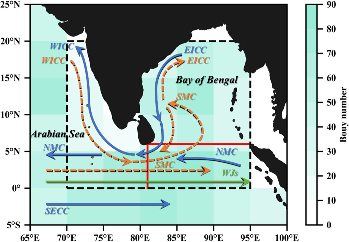
Figure 1. The surface circulation system of the North Indian Ocean is in the study area. The orange dashed line and blue line indicate the main paths of the surface currents during the summer monsoon and winter monsoon periods, respectively. SMC, Southwest Monsoon Current; NMC, Northeast Monsoon Current; WICC, West Indian Coastal Current; EICC, East Indian Coastal Current; SECC, South Equatorial Counter Current. The green line indicates the main currents during the monsoon transition period, WJs, Wyrtki Jets. The red line shows the 6° N section at the mouth of the Bay of Bengal and the 81° E section in the central equatorial seas, respectively, and the black dashed rectangular box shows the spectral clustering area. Cyan shading indicates the number of Argo buoys distributed in the 5°×5° grid from January 2011 to December 2020 in the study area.

In fact, the distribution and water exchange characteristics of ASW and BBW in the circulation system are difficult to characterize directly due to the complexity of the changes in upper ocean processes (De Vos et al., 2014). Previous studies are usually limited to single cruise observations, focusing on the ocean dynamics mechanism in the Sri Lankan region but failing to provide a comprehensive answer to the expansion paths of ASW and BBW as well as the spatiotemporal characteristics of the water exchange on an interannual basis. Moreover, the current distribution range of the upper water masses is mostly based on the thermohaline criterion, and more effective and accurate methods of water mass analysis have not been introduced, which leads to a lack of intuitive expression of the distributions of ASW and BBW in the seasonal process (Jensen et al., 2016; Cullen and Shroyer, 2019; Hormann et al., 2019). With the continuous optimization and development of classification methods, spectral clustering (SC) has demonstrated good performance in water mass analysis and water exchange studies, providing the possibility to clearly understand the seasonal distribution and movement state of water masses (Song et al., 2011). Different from the traditional clustering methods, SC, based on the theory of image analysis, fully considers the variability between target data points and the distribution structure of the overall temperature and salt data in the water mass classification study combined with a T-S diagram, and has successfully analyzed the Kuroshio water and shelf water in the East China Sea, as well as the water exchange between the Bohai Sea and the Yellow Sea during the winter gales (Li et al., 2015; Song et al., 2016a), but it has not been applied in larger scale regions.

Therefore, from the perspective of water mass analysis, we highlight the differences in the nature and the extent of the mixing region between the ASW and BBW in the Northern Indian Ocean and reveal the seasonal distribution of the upper water masses and their movement paths through the SC method to explore the water exchange process between the ASW and BBW in the main channel. Based on Argo and SODA data, we focus on the distribution of upper water masses and the spatiotemporal characteristics of water exchange from 2001 to 2020.

2 Data and methods

2.1 Data

2.1.1 Argo

The T-S diagram of seawater combined with measured data can visualize the temperature and salinity properties of seawater masses and has been widely used to study the delineation and mixing of water masses (Li et al., 2004; Zang et al., 2020). In this paper, we use the quality-controlled Argo temperature and salinity data provided by the Global Argo Data Center (http://www.argo.org.cn/) to preliminarily study the temperature and salinity distributions of the upper water masses such as ASW and BBW and to determine the main sea areas where the ASW and BBW are mixing. Since the international Argo program was largely stabilized after the initial construction of the observation network at the end of 2007, we use here Argo data for the period from January 2011 to December 2020, with the pressure range of the buoy observations set to 0–200 dbar. The spatial distribution of the number of Argo buoys by 5° × 5° is shown in Figure 1, and the corresponding thermohaline dataset is shown in Figure 2. The final information includes all the thermohaline scattering data from 1563 buoys in the range of 65° E–100° E, 5° S–25° N.

Figure 2

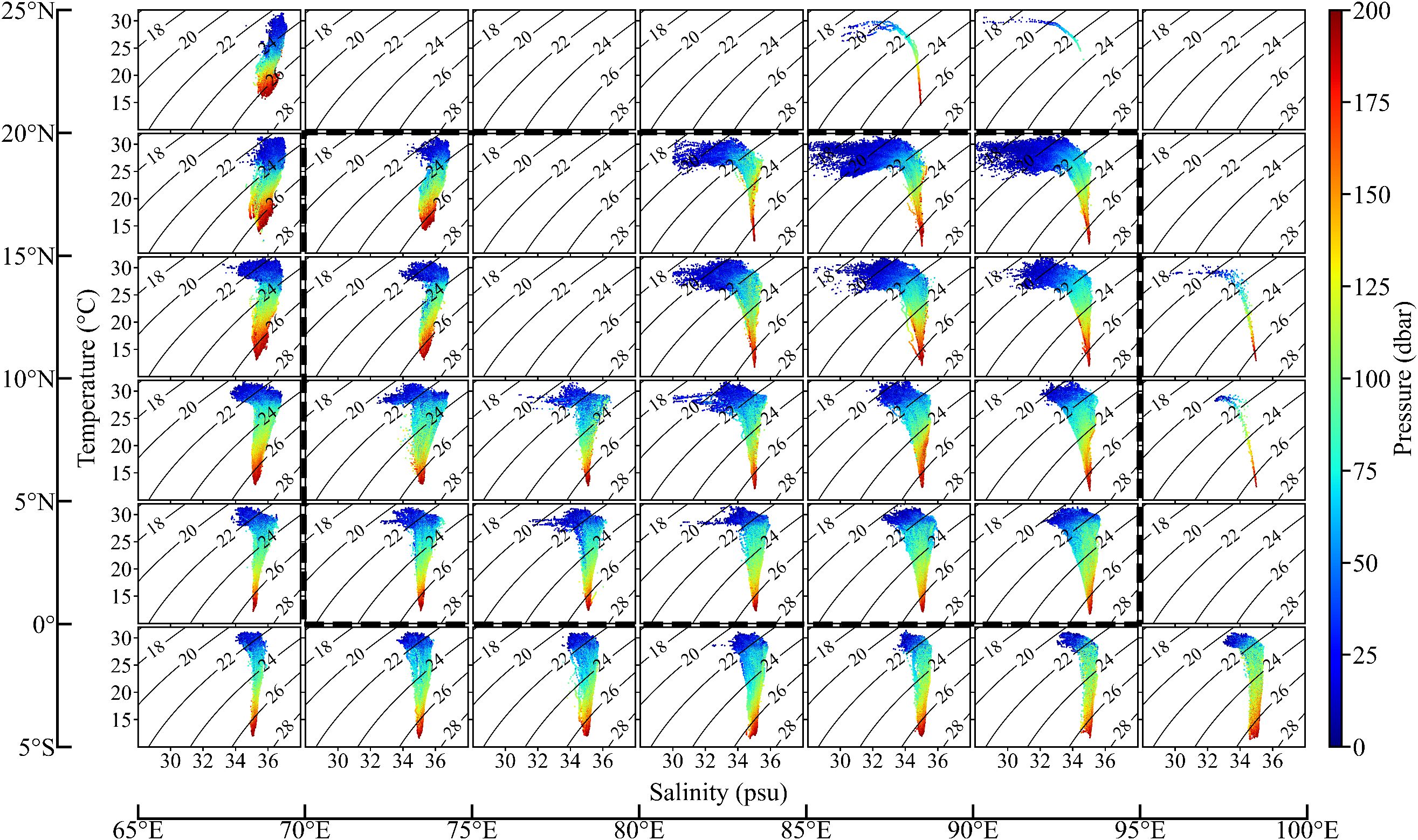
Figure 2. T-S diagram of the upper waters of the North Indian Ocean in the study area. The subplot represents the data within the 5° × 5° grid defined in Figure 1, the color indicates the pressure (dbar), and the contour lines are the potential density (kg/m³).

According to Figure 2, the temperature characteristics of the seawater in the northern Indian Ocean are relatively consistent in the range of 0–200 dbar, decreasing gradually from the surface downwards, and are mostly in the range of 10–32°C. There is a significant difference between the salinity of seawater on the east and west sides of the Indian Peninsula in the range of 0–100 dbar, and the salinity of the upper layer of seawater to the west of 75° E and north of 15° N is at the maximum overall, with part of it exceeding 36, which is the source area of ASW; on the contrary, the salinity of seawater to the east of 80° E and north of 15° N is lower, and the salinity of surface seawater can be lower than 30, which represents the center of BBW. The gradual mixing of ASW and BBW is observed in the range of 0–10° N in the central part of the range, i.e., the southern tip of the Indian Peninsula, where the difference in salinity of seawater is significantly smaller, especially between 75 and 80° E, suggesting that the ASW and BBW mixing takes place mainly in the latitudinal channel between southern Sri Lanka and the equator, with the 0–5° N range in the central sea as the center of east–west water exchange.

South of the equator (0–5° S), the shape of the T-S diagram of seawater tends to be consistent, and the thermohaline nature is essentially unchanged over the horizontal and vertical distribution ranges, with salinities mostly in the range of 34–35, which is characteristic of Indian Equatorial Water (IEW) (Stramma et al., 1996). Therefore, to focus on the movement process of ASW and BBW under the action of monsoon and equatorial current systems, the source and mixing zones containing ASW and BBW are determined in this paper to be in the range of 70–95° E, 0–20° N, i.e., the region where the two water masses are seasonally classified, as shown by the black dashed rectangular box in Figures 1, 2.

2.1.2 SODA

SODA (Simple Ocean Data Assimilation) reanalysis data are based on the Modular Ocean Model (MOM) and Parallel Ocean Program (POP) of the Geophysical Fluid Dynamics Laboratory (GFDL), using parallel algorithms to perform static equilibrium and Boussinesq approximation on three-dimensional original equations. The dataset includes physical quantities such as salinity, temperature, current velocity, sea surface height, and sea surface wind stress (Carton et al., 2000; Carton and Giese, 2008). SODA3 is often used to reproduce and compare large-scale latitudinal currents, especially equatorial and boundary currents (such as WJs), and is stable in trend analysis, seasonal changes and water mass structure (Wang et al., 2012; Feng et al., 2025; Rahman and Rahaman, 2024). The spatial resolution of SODA3.15.2 (http://dsrs.atmos.umd.edu/DATA/soda3.15.2/REGRIDED/ocean/) is 0.5°×0.5°, and the vertical stratification is 50 layers. The time range of SODA3.15.2 data selected in this paper is from January 2001 to December 2020, focusing on the study of the differences in seawater salinity and current velocity in the upper 100m depth, as well as the seasonal clustering analysis of water masses in the characteristic depth layer.

The contour profiles of salinity and current velocity in the annual mean 0–100 m depth range at the mouth of the Bay of Bengal in the 6°N latitudinal direction and in the central equatorial sea in the 81°E longitudinal direction are given in Figure 3. Compared with the equatorial section, the spatial variations in salinity are more obvious in the Bay mouth area, with the annual average seawater salinity being higher in the west and lower in the east, and the current direction west of 85° E shows a characteristic of the east in and west out, manifested as the long-term influence of SMC and NMC on the western channel of the Bay mouth. The southward current is dominant in the eastern part of the Bay mouth, but a northward current exists perennially above the eastern boundary at a depth of 30 m. The equatorial section shows that the salinity of seawater from south of Sri Lanka to the equator is generally high, with a gradual increase from north to south, which is influenced by the westward transportation of freshwater in the north and the high salinity water driven by WJs in the equator in the south, which can be corroborated by the surface westward currents north of 4.5° N and strong eastward currents at the equator (0–2° N).

Figure 3

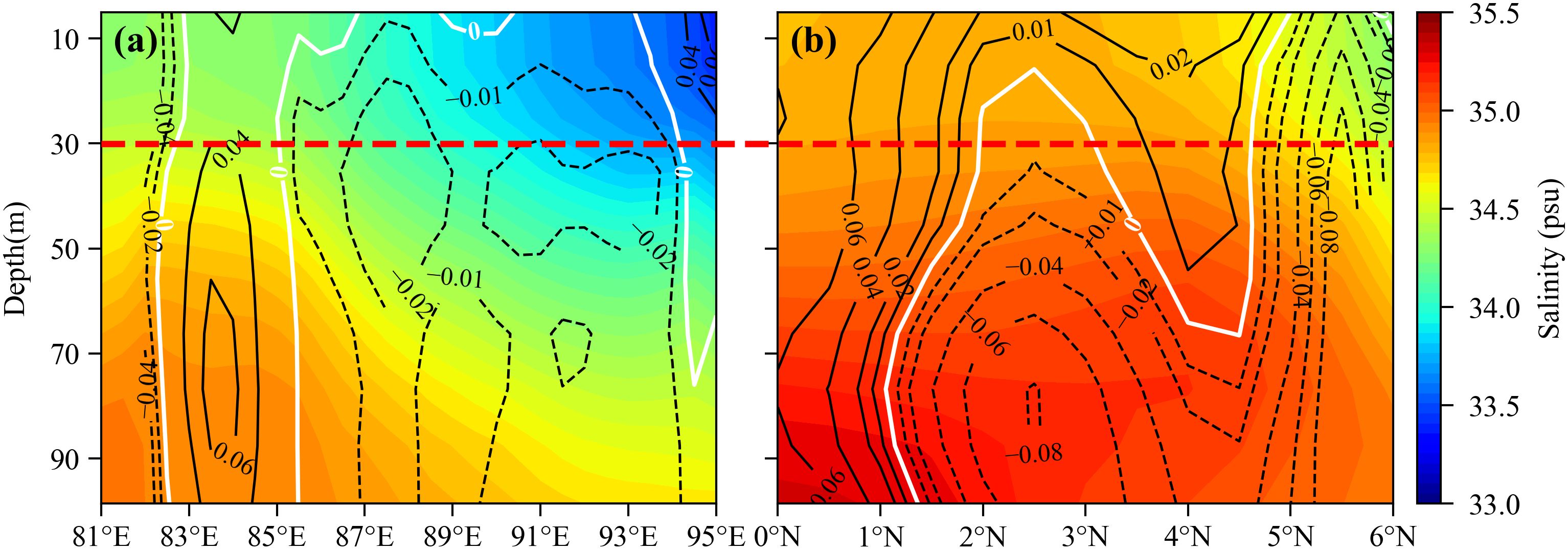
Figure 3. Upper 100 m profiles of salinity and current velocity at 6° N (a) and 81°E (b) under the annual mean. Current velocity (m/s) contours with positive values for north–and eastward currents and negative values for south–and westward currents. The red dashed line is the 30 m characteristic depth layer.

Therefore, according to the two upper profiles in the Bay mouth and the equatorial region, it can be seen that the salinity properties of seawater in the range from the surface to 30 m depth are more obvious and are more significantly affected by the North Indian Ocean current system, especially the low salinity BBW captured at 30 m depth and shallower in the eastern part of the Bay mouth and its transport to the south (outside the Bay) (Figure 3a). In general, the difference in water masses is most obvious in the surface layer, and the core of BBW is also mainly located in the surface layer, but even so, we consider the distribution range of the entire upper water mass because ASW is distributed at the depth of 0–100 m in comparison (Schott and McCreary, 2001), so it is necessary to select a suitable depth layer as a representative for SC analysis. Based on the T-S diagram given in Figure 2, it can also be concluded that at depths of 25 m and shallower, the difference in salinity between the upper water masses ASW and BBW is more pronounced, but the properties of the seawater tend to be similar in deeper ranges, with greater reproducibility of their respective temperature and salinity data, which may increase the likelihood of confounding of the different water masses in the clustering analysis.

Consequently, in order to better represent the distribution of the upper water mass, we select the characteristic depth layer of 30 m to conduct the SC analysis of the water mass (as shown by the red dashed line in Figure 3). This depth layer reduces the impact of surface disturbances and the possible overlap of deeper seawater in the data, making it more accurate and representative.

2.2 Methods

2.2.1 Spectral clustering

Based on the seawater temperature and salt level structure on the characteristic depth layer, we refer to the spectral clustering (SC) method to categorize the upper water masses (Von Luxburg, 2007) and give the motion state of each water mass during the seasonal change process, and the operation steps of SC are as follows (Equations 1–4):

(1) For a given thermohaline dataset X = {x₁,…, x_n}, first calculate the similarity matrix W (here, the thermohaline dataset consists of seawater temperature and salinity variables at the 30 m depth layer in the study area), each element of which W_ij denotes the similarity between data points x_i and x_j. The similarity matrix is often defined using a Gaussian kernel function:

$\begin{array}{ll}{W}_{ij}=\text{ex}p(-\frac{\Vert x_i-x_j{\Vert }^2}{2{\sigma }^2})& (1)\end{array}$

where σ is the width parameter of the Gaussian kernel, which represents the scale of the similarity measure;

(2) Define the diagonal matrix D and the Laplacian matrix L:

$\begin{array}{ll}{D}_{ii}={{\displaystyle \sum }}_j{W}_{ij}& (2)\end{array}$

$\begin{array}{ll}L=D^{-\frac{1}{2}}L{D}^{-\frac{1}{2}}& (3)\end{array}$

where D_ii denotes the sum of all values in row i of matrix W;

(3) Solve the matrix L to obtain the minimum k eigenvalues (λ₁,…,λ_k) and the eigenvectors corresponding to these k eigenvalues ($\overline{x}$₁,…, x_k);

(4) Construct the target matrix O = (($\overline{x}$)₁,…, ($\overline{x}$)_k) ∈ R^n×k, each of whose columns is equal to each of the eigenvectors obtained in the previous step, respectively;

(5) Normalize each row of the matrix O separately so that it has a uniform unit criterion and construct the matrix Q ∈ R^n×k:

$\begin{array}{ll}{O}_{ij}=\frac{O_{ij}}{{({{\displaystyle \sum }}_j{O}_{ij}^2)}^{\frac{1}{2}}}& (4)\end{array}$

(6) Consider each row of matrix Q as each corresponding data point; Q is a matrix with N data points and k parameter attributes for each data point. Finally, this newly constructed set of data points is clustered using the K-means cluster analysis method, which in turn yields each corresponding cluster and its center.

The clustering results are sensitive to the Gaussian kernel width parameter (σ) and the number of clusters. Since the temperature and salinity point data involved in the clustering have been standardized, we set σ in step (1) to 1 (Song et al., 2011; Song et al., 2016b). The number of clusters is based on the T-S diagram distribution in Figure 2. We set the number of clusters in the study area including IEW to 3, and the number of clusters in the main mixing area of ASW and BBW (black dashed area) to 2.

To verify the accuracy of this method, we first conducted SC analysis on the study area (65–100° E, -5–25° N) including most of the upper ocean current systems using the annual average temperature and salinity data of SODA3.15.2 at a depth of 30 m (Figure 4). Figure 4a shows the horizontal distribution structure of the upper water masses, and Figure 4b is the corresponding T-S diagram. The water masses in the study area are clustered into 3 categories, and the horizontal distributions of ASW and BBW are more fluctuating due to the influences of the monsoon circulation and equatorial current system. The mixed water of ASW and BBW during seasonal changes is categorized as IEW on the annual average. The clustering results show that part of the ASW has a low temperature relative to the IEW and BBW, and the highest salinity, which reflects the geographical location of the Arabian Sea in the horizontal distribution; the BBW has the largest range of temperature and salt distribution, with the salinity spanning from 29 to 34, and the location of the water mass is distributed north of 5° N overall, in the inner Bay of Bengal; IEW is the most concentrated, with a salinity profile roughly 34–35, mostly within the equatorial waters of 5° S–5° N. In terms of structure, the results of SC analysis are similar to the properties and horizontal distribution results of the upper water masses in the North Indian Ocean given by Emery et al. and Sardessai et al (Emery, 2001; Sardessai et al., 2010). In addition, we also mapped the spectral clustering results into the spectral clustering feature space constructed by the first two eigenvectors of the graph Laplacian matrix (Supplementary Figure S1). The identified clusters are clearly separated in the spectral feature space and show a clear nonlinear curved structure. This phenomenon indicates that the water masses are not discretely distributed, but form a continuous transition along the temperature and salinity gradient, which further illustrates the applicability of the SC method in the classification of water masses.

Figure 4

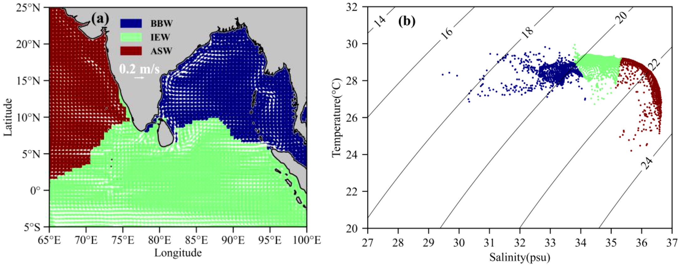
Figure 4. SC results of the 30 m depth layer in the North Indian Ocean in the study area under annual mean. (a) The structure of the upper water mass distribution in the study area, with white arrows showing the 30 m depth layer flow field; (b) the corresponding T-S diagram, where the same color corresponds to the same range of data point sets in (a).

It is worth noting that Figure 4 shows the clustering result under the long-term average, reflecting the relatively conservative geographical spatial distribution of water masses. However, according to the Argo measured data in Figure 2, only the temperature and salinity of seawater south of the equator (0-5° S) are stably maintained as the IEW structure, while the IEW north of the equator actually reflects the mixing process of ASW and BBW during the seasonal process. Therefore, in Section 3.1, we follow the previously defined clustering region and choose the number of clusters to be 2 for SC analysis, with the aim of clearly capturing the movement and extent of expansion of ASW and BBW during the seasonal process.

2.2.2 Water flux calculation

The mouth of the Bay of Bengal and the central equatorial seas are within the main channel where ASW and BBW undergo exchanges. To study the material exchange relationship between ASW and BBW during their movements, water transport calculations were carried out for the upper 100m section at 6° N of the Bay mouth and 81° E of the equator according to the water flux calculation formula (Equation 5) (Qiu and Zhu, 2015).

$\begin{array}{ll}{F}_v={{\displaystyle \sum }}_i\left[\Delta l_i{{\displaystyle \sum }}_k{v}_{i,k}\Delta z_k\right]& (5)\end{array}$

where i and k are the horizontal and vertical grid numbers in the section, respectively; v_i,_k is the normal current velocity at the center of the grid (i,k), positively oriented to the north and east; Δl_i and Δz_k are the width and thickness of the (i,k) grid; and the water flux is in units of Sv (1Sv = 10⁶m³/s).

The flux estimates are derived from the SODA reanalysis. To validate the meridional ocean current velocities, we selected two nearby RAMA buoys located along the 6° N section (at 90° E, 4° N and 90° E, 8° N), both at a depth of 10 m. The validation results show good agreement (Supplementary Figure S2).

3 Results

3.1 Seasonal distribution and movement of water masses

The SC results show the distribution and motion processes of ASW and BBW during seasonal changes. According to Figure 5, the motions of the upper water masses under each period show a clear connection with the prevailing circulation pattern. In January, the NMC and the southward EICC connected with the WICC in the Arabian Sea, constituting a link for the BBW out of the Bay. The BBW can expand westward along this channel to 73° E, and the other part of the low salinity water continues to move northward along the west coast of the Indian Peninsula. As the winter monsoon receded, the influence of the NMC gradually weakened in April, and although the westward current is still dominant in the mouth of the Bay of Bengal, its intensity decreased significantly, which led to the contraction of the BBW into the Bay. At the same time, the spring WJs transport the upper layer of water eastward, which makes the distribution of ASW wider. In July, the sea is controlled by a strong summer monsoon, and the southeastward WICC converges with the SMC around 5° N, forming a strong northeastward current in the southern part of the Bay mouth. The main body of the SMC can bring the ASW to a range of 10° N inside the Bay, and some of them continue northward along with the EICC. During this period, the distribution range of ASW reaches its peak, compressing the space of BBW to the greatest extent. Affected by the invasion of ASW, BBW moves out of the Bay with the southward current in the eastern part of the Bay, and this trend continues until autumn. In October, the spreading range of BBW in the east increased further, forcing the ASW to contract in a southwesterly direction, and the invasion of ASW in the Bay subsided, and the BBW regained the dominant position in the eastern sea area.

Figure 5

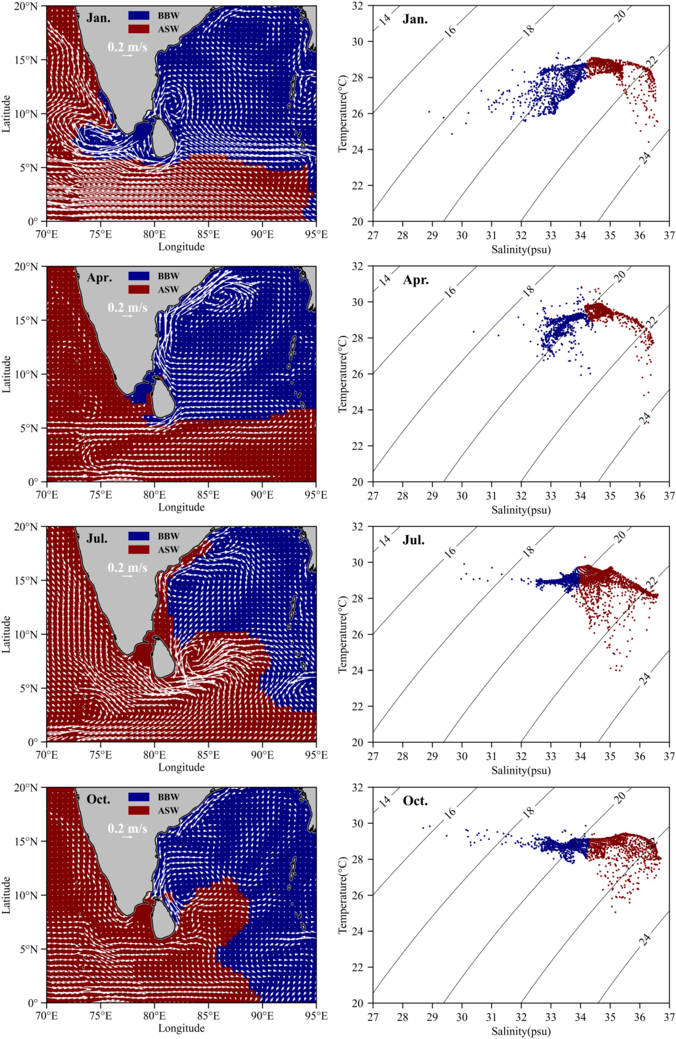
Figure 5. SC results of ASW and BBW at 30m depth under the average of January, April, July, and October. The left panel shows the distribution state of water masses, and the white arrows show the 30m depth layer flow field; the right panel shows the T-S diagram of the corresponding water masses.

Correspondingly, the T-S diagram shows the temperature and salinity distribution and clustering process of ASW and BBW. BBW shows more obvious seasonal variations, with the widest distribution of temperature and salt structure during the winter monsoon period, reflecting the westward expansion of BBW into the Arabian Sea during this period; on the contrary, the surface BBW in the temperature and salt ranges within the characteristic values of 28–30°C and 32–34 during the summer monsoon period, and the relatively cooler and saltier ASW gained most of the dataset space. The difference in properties during the monsoon transition period is mainly reflected in the salinity, which takes 34.5 as the dividing line and has a more consistent shape, which is the result of mixing in the absence of strong seasonal currents in the transition state.

In addition, based on the clustering results, we analyze the degree of attribution of seawater according to the core location of ASW and BBW in each season to further explain the mixing process of water masses (Supplementary Figure S3). The results show that the mixing zone is narrower and the attribution of the water masses is clearer during the monsoon period, which further proves the strong influence of the monsoon currents on the region, and the mixing zones of the water masses in the spring and autumn are more irregular in comparison, while at the same time, the variation of the core positions of the water masses indicates the corresponding movement trend of the water masses.

3.2 Spatiotemporal characteristics of water exchange and the mechanisms

Schematic illustration of the expansion pathways of ASW and BBW given by the seasonally averaged SC results. Figure 6 shows that ASW invades the BBW during the southwest monsoon mainly through two pathways, i.e., the main portion carried by the SMC and the northward branch along the EICC, both pathways cross the equatorial central Indian Ocean at 81° E and the mouth of the Bay of Bengal at 6° N section, and during the seasonal transitions, the WJs also transport the ASW eastward, which is a major source of eastward water fluxes on the equatorial section. The dispersal process of BBW also has two different pathways, one is westward into the Arabian Sea in winter through the channel formed by EICC, NMC, and WICC, and the other is transported to the outer sea in the eastern part of the Bay mouth in summer and autumn. These pathways are also verified in the seasonal distribution of Argo buoys (Supplementary Figure S4).

Figure 6

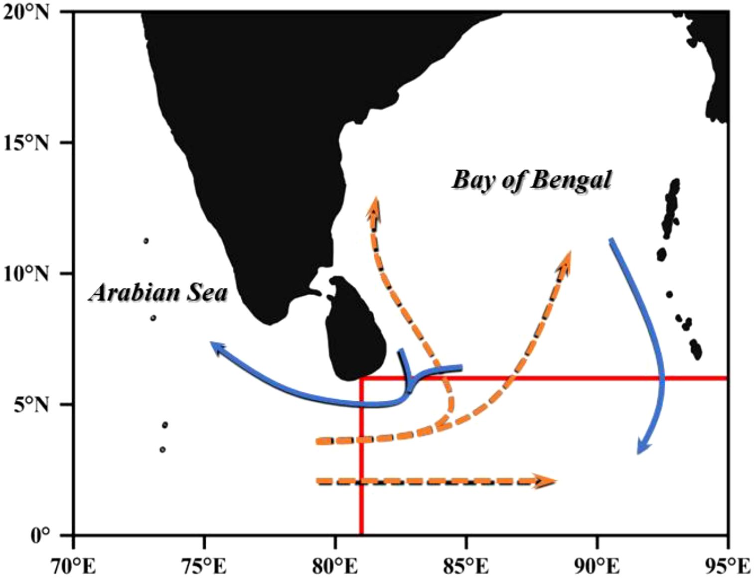
Figure 6. Water masses movement paths under SC results. The orange dashed line and the blue line are the schematic expansion paths of ASW and BBW, respectively, and the red line is the location of the two sections given in the previous section.

Thus, the two sections at 6° N in the Bay of Bengal and 81° E in the central equatorial seas become the necessary pathways for the mixing and exchange of ASW and BBW during the seasonal changes, and the changes in water fluxes at the cross sections are also important indicators of the water exchange characteristics.

The monthly average data from 2001 to 2020 calculated in this paper show a generally positive correlation with the time series of water and net water flux at a depth of 100 m on the two sections (Figure 7). Typically, due to the influence of strong SMC crossing the equatorial bottleneck and bringing a large amount of ASW into the Bay of Bengal, the change in water flux in the equatorial section will be earlier than that in the section at the mouth of the Bay. This trend is reversed in winter due to NMC. Therefore, there is an asynchrony in the changes in water flux in the two sections during the season, which is particularly noticeable in the summer to autumn season.

Figure 7

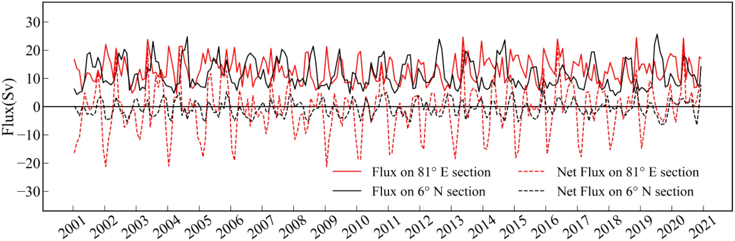
Figure 7. Changes in water flux and net water flux at monthly intervals from 2001 to 2020. Water fluxes across the 6° N and 81° E sections are shown by solid black and red lines, respectively; net water fluxes are shown by dashed black and red lines, with positive values for north- and eastward-flowing water fluxes and negative values for south- and westward-flowing water fluxes.

Table 1 shows the results of water flux and net water flux in each period. Monsoon currents and WJs have a more significant impact on the water exchange process in the central equatorial seas, with water fluxes across the equatorial section reaching an average of 12.97 ± 2.58 Sv and 11.32 ± 2.70 Sv in the Bay mouth section. In terms of seasonal variability, the water exchange processes in the Bay mouth area are more active during the summer winds (17.13 ± 1.95 Sv), with water flux variations that exceed those of the equatorial waters in some years (2001, 2007, 2012, 2014, 2019), which is likely related to the large transport of BBW in the eastern part of the Bay mouth during summer and autumn. The annual average of low salinity water outflow from the Bay of Bengal reaches 6.03 ± 1.50 Sv, but the Bay mouth section presents higher values of net outflow in June-September each year, suggesting that BBW is transported more in the summer and autumn than in the winter, According to the research of Madkaiker et al., this is attributed to the equatorward-flowing EICC during summer, which transports low salinity water from the Bay of Bengal to regions outside the Bay (Madkaiker et al., 2024). For the equatorial region, the main variability consists of the monsoon currents, followed by the influence of WJs. In winter and spring, the water flux across the equatorial section is almost exclusively from the NMC-driven westward current, with a mean net water flux of 16.43 ± 1.48 Sv in January; this corresponds to the peaks of the eastward net flux alternating between the April–May and September–November periods in the interannual scales, reflecting changes in the strength of the WJs in the spring and the autumn over the long period during the seasonal transition. Overall, the trend in net water fluxes at the Bay mouth section is generally consistent with the performance at the equatorial section, with roughly a 1–2-month time lag, but the magnitude of the change is much smaller than the latter.

Table 1

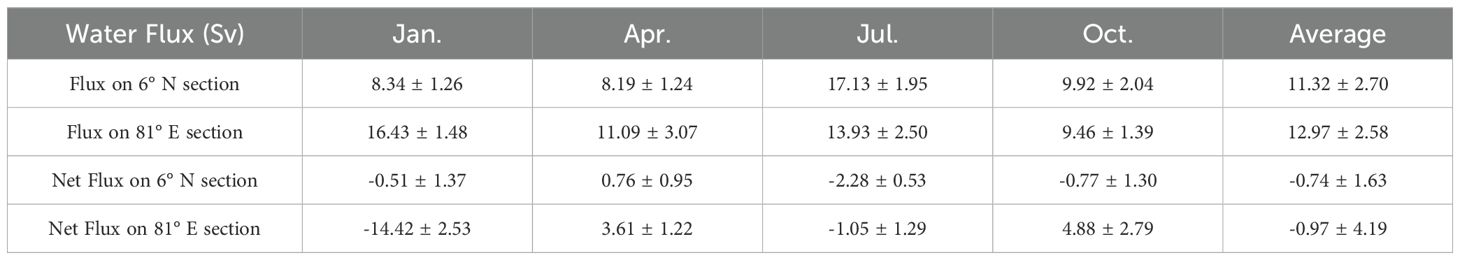
Table 1. The average results of water flux and net water flux on the sections in different periods.

The changes in the four fluxes with time are analyzed by spectral correlation. Figure 8 shows that the time series of each flux from the Bay mouth and on the equatorial section have distinct semiannual and 1-year cycles, suggesting that the monsoon transition process in the Northern Indian Ocean and the influence of the equatorial anomalous westerly winds and the Kelvin wave propagation in the semiannual cycle are the main mechanisms controlling the exchange and mixing between the ASW and the BBW. The cycle of water fluxes on the equatorial section is more complex, and the influence of MISO may be a contributing factor to the intra-seasonal cycle variation it exhibits in 2–3 months (Webber et al., 2014; Krishnamurti et al., 2017). In longer time scales, water flux variations at the equator and Bay mouth sections also manifest a 2–3 year cycle, which may be related to changes in the equatorial latitudinal winds and sea surface current field induced by a shift in the cycle of IOD events (Luo et al., 2007; Hashizume et al., 2013).

Figure 8

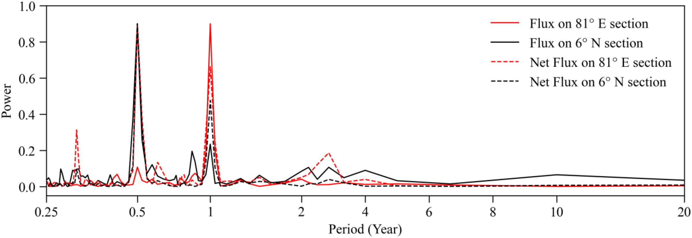
Figure 8. Results of the spectral analysis of the water flux and net water flux curves with time for the 6° N and 81° E sections.

The Dipole Mode Index (DMI) is defined as the difference in sea surface temperature anomalies between the tropical western Indian Ocean (10° S–10° N, 50–70° E) and the southeastern Indian Ocean (10°–0° S, 90–110° E), and is the primary indicator for measuring the intensity of IOD events (Saji et al., 1999). Zhang et al. (2013) classified IOD events as pIOD (or nIOD), based on the amplitude of the DMI greater than (or less than) one positive (negative) standard deviation. Figure 9 shows the time series of the southward transport anomaly (a) on the Bay mouth section and the westward transport anomaly (b) on the equatorial section versus the DMI from 2001 to 2020.

Figure 9

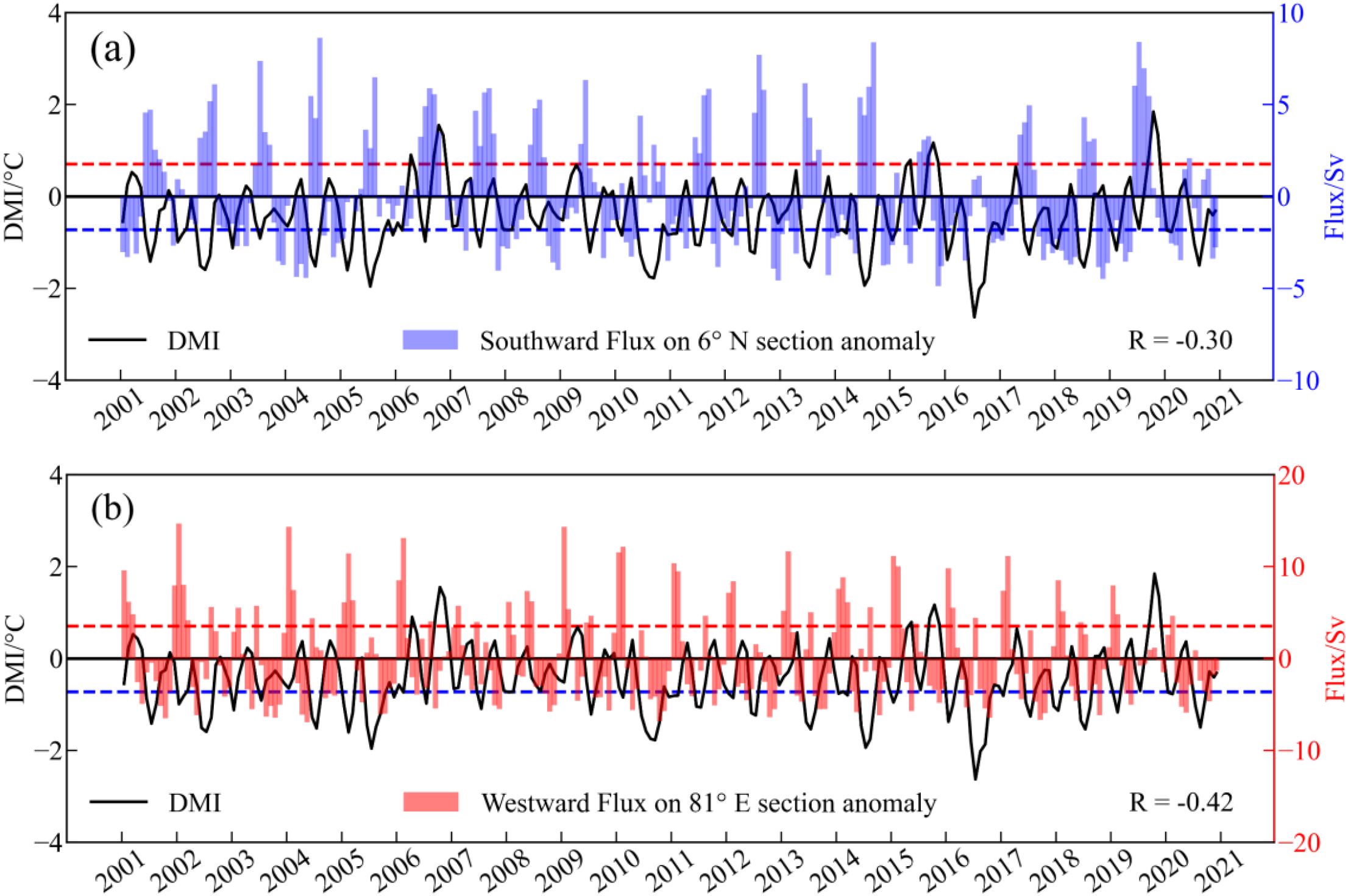
Figure 9. Time series of anomaly and Dipole Mode Index (DMI) for southward and westward transport in the Bay Mouth section (a) and equatorial section (b). R is the correlation coefficient between transport anomalies and DMI (over 99% confidence level), and the red and blue dashed lines are positive and negative 1× standard deviation of the DMI series, respectively.

In most nIOD years (2005, 2010, 2014, 2016), the amount of low salinity water passing through the mouth of the Bay and the central equator increased significantly, which manifested itself as a continuous spreading of BBW to the outer Bay and equatorial waters. Similar findings by Dandapat et al. indicate that during negative nIOD events, equatorial westerly wind anomalies enhance the propagation of downwelling Kelvin waves, which in turn strengthen the cyclonic circulation in the western Bay of Bengal. This process further promotes the development of a stable and intensified equatorward EICC, thereby facilitating the efficient southward transport of low salinity water from the northern Bay (Dandapat et al., 2018). This process is also captured by the abnormally strong southward current in the western mouth of the Bay during the nIOD in Supplementary Figure S5. The barrier layer formed by the large low salinity water exacerbated the warming of the upper ocean waters in the eastern Indian Ocean, responding positively to the course of the nIOD event on an interannual basis (Kumari et al., 2018). On the contrary, in pIOD years (2006, 2015, 2017, 2019), the delivery of low salinity water to the equatorial Indian Ocean is lower than the average. Equatorial easterly wind anomalies cause missing Kelvin waves and eddy activity, which weaken the freshwater transport capacity of the EICC (Supplementary Figure S5), resulting in a thinning of the thickness of the eastern barrier layer and a consequent weakening of the impacts of the sea-air interaction it causes (Dandapat et al., 2018). Correspondingly, the transport anomaly and DMI are negatively correlated in both sections, with correlation coefficients of −0.30 and −0.42, respectively, and the change in transport in the equatorial section seems to be more sensitive to IOD events, with a more complex magnitude of change in the interannual period. (Figure 9).

4 Conclusions and discussions

Based on the Argo and SODA data from 2001 to 2020, we determine the extent and seasonal distribution of the mixing zone of ASW and BBW, give the kinematic state and water exchange process of ASW and BBW in the North Indian Ocean circulation system through the SC method, and analyze in detail the spatiotemporal characteristics of the water exchange and its control mechanism.

The SC results show that the seasonal distribution of the upper water masses in the study area varies obviously. The distribution range of ASW peaks in summer, which can invade the north of 10° N within the Bay of Bengal, and its eastward expansion path is mainly provided by SMC and WJs; BBW reaches the region west of 73° E in the Arabian Sea in winter along with the NMC and then spreads a lot in the eastern part of the Bay mouth to the equatorial Indian Ocean in summer and autumn. The thermohaline nature of BBW changes more significantly than ASW during the seasonal process.

The time series from 2001 to 2020 reveals that the changes in water and net water flux on the Bay mouth and equatorial sections show a general positive correlation, but the water exchange process in the equatorial region is more complex, with an annual average water flux of 12.97 ± 2.58 Sv, which is larger than that on the Bay mouth (11.32 ± 2.70 Sv). The westward current driven by the NMC reaches 16.43 ± 1.48 Sv in winter and spring, corresponding to the peak eastward water flux (13.93 ± 2.50 Sv) that occurs alternately in summer and autumn, showing a clear seasonal variation. For the Bay mouth, BBW transport is an important factor that reflects the water exchange process. The results show that the annual average of low salinity water outflow from the Bay of Bengal is 6.03 ± 1.50 Sv, and it is larger in summer and autumn than in winter, indicating that the water exchange process in the mouth of the Bay of Bengal is more active during the summer monsoon period. In addition, the intensity of WJs shows significant variations during the seasonal transition in different years, further exacerbating the differences in water exchange between the equatorial and Bay mouth regions.

The continuously circulating upper ocean processes significantly affect the periodic changes in water fluxes, especially in the semiannual and 1-year cycles, suggesting that the monsoon transition process in the northern Indian Ocean and the influence of equatorial semiannual Kelvin waves are the main factors driving the exchange and mixing between ASW and BBW. On interannual scales, water exchange in the equatorial region and the Bay mouth region also shows a clear connection with IOD events, reflecting a 2–3-year cycle. A comparison of the low salinity water transport anomalies with the DMI time series at the two sections reveals a negative correlation (−0.30 and −0.42), and changes in transport at the equatorial section appear to be more sensitive to IOD events, with more complex magnitudes of change on the interannual scale.

The distribution of water masses and water exchange processes between the Arabian Sea and the Bay of Bengal are of great significance for the thermohaline balance of the North Indian Ocean (Madkaiker et al., 2024). Based on this study, we show to some extent the applicability of the SC method in the classification of upper water masses in the North Indian Ocean and find that there are significant seasonal and interannual differences in the water exchange capacity of the two regions, and that such mutual water exchange processes and the expansion paths of the water masses therein make important contributions to the ecology of neighboring oceans as well as to the development of the fishery industry, particularly along the coasts of the Indian Peninsula and Sri Lanka. In addition to this, measurements and analysis of the low salinity water of the Bay of Bengal passing over the two main passages at the mouth of the Bay and in the central equator can also help in the assessment and prediction of climatic anomalies such as the IOD.

However, it is worth noting that the SC method based on the T-S diagram helps in the identification and characterization of water masses, but with the continuous development of water mass analysis work, more parameters are being applied to new studies, such as spicity function, dissolved oxygen, and nutrient salt concentration (Peña-Izquierdo et al., 2015; Lao et al., 2022; Zhou et al., 2023). Therefore, relying only on the temperature and salinity structure for cluster analysis may be slightly insufficient, and the introduction of relevant marine biochemical and physical parameters in future work will further enhance the objectivity and accuracy of the water mass analysis results and provide a more comprehensive perspective for regional water mass analysis. In addition, the dependence of the SC method on parameter settings, the accuracy limitations of the SODA reanalysis used in the water mass analysis, and the uneven spatial distribution of some Argo buoys may constitute objective sources of uncertainty in this study.

Data availability statement

The datasets presented in this study can be found in online repositories. The names of the repository/repositories and accession number(s) can be found in the article/Supplementary Material.

Author contributions

DZ: Visualization, Writing – original draft. YF: Data curation, Formal analysis, Writing – review & editing. JG: Funding acquisition, Project administration, Resources, Writing – review & editing. JS: Conceptualization, Methodology, Writing – original draft, Writing – review & editing. YC: Software, Validation, Writing – review & editing.

Funding

The author(s) declare that financial support was received for the research and/or publication of this article. Dalian Science and Technology Innovation Fund (2024JJ11PT007), Dalian Science and Technology Program for Innovation Talents of Dalian (2022RJ06), Science and Technology Plan of Liaoning Province (2024JH2/102400061), Provincial Education Department Scientific Research Platform Construction Project (LJ232410158056).

Acknowledgments

We would like to thank the Dalian Ocean University Branch of the National Marine Data Center, Liaoning Ocean and Polar Science Data Center, and Dalian Ocean Science Data Center for providing data support.

Conflict of interest

The authors declare that the research was conducted in the absence of any commercial or financial relationships that could be construed as a potential conflict of interest.

Generative AI statement

The author(s) declare that no Generative AI was used in the creation of this manuscript.

Publisher’s note

All claims expressed in this article are solely those of the authors and do not necessarily represent those of their affiliated organizations, or those of the publisher, the editors and the reviewers. Any product that may be evaluated in this article, or claim that may be made by its manufacturer, is not guaranteed or endorsed by the publisher.

Supplementary material

The Supplementary Material for this article can be found online at: https://www.frontiersin.org/articles/10.3389/fmars.2025.1610528/full#supplementary-material

References

Carton J. A., Chepurin G., Cao X., and Giese B. (2000). A simple ocean data assimilation analysis of the global upper ocean 1950–95. Part I: Methodology. J. Phys. Oceanogr. 30, 294–309. doi: 10.1175/1520-0485(2000)030<0294:ASODAA>2.0.CO;2

Crossref Full Text | Google Scholar

Carton J. A. and Giese B. S. (2008). A reanalysis of ocean climate using Simple Ocean Data Assimilation (SODA). Monthly weather Rev. 136, 2999–3017. doi: 10.1175/2007MWR1978.1

Crossref Full Text | Google Scholar

Cullen K. E. and Shroyer E. L. (2019). Seasonality and interannual variability of the Sri Lanka dome. Deep Sea Res. Part II Top. Stud. Oceanogr. 168, 104642. doi: 10.1016/j.dsr2.2019.104642

Crossref Full Text | Google Scholar

Dandapat S., Chakraborty A., and Kuttippurath J. (2018). Interannual variability and characteristics of the East India Coastal Current associated with Indian Ocean Dipole events using a high resolution regional ocean model. Ocean Dynamics 68, 1321–1334. doi: 10.1007/s10236-018-1201-5

Crossref Full Text | Google Scholar

De Vos A., Pattiaratchi C. B., and Wijeratne E. M. S. (2014). Surface circulation and upwelling patterns around Sri Lanka. Biogeosciences 11, 5909–5930. doi: 10.5194/bg-11-5909-2014

Crossref Full Text | Google Scholar

Emery W. J. (2001). Water types and water masses. Encycl. Ocean Sci. 6, 3179–3187. doi: 10.1006/rwos.2001.0108

Crossref Full Text | Google Scholar

Feng Q., Zhou J., Han G., and Xie J. (2025). Variation of wyrtki jets influenced by indo-Pacific ocean–atmosphere interactions. J. Mar. Sci. Eng. 13, 691. doi: 10.3390/jmse13040691

Crossref Full Text | Google Scholar

Han W. and McCreary J. P. Jr. (2001). Modeling salinity distributions in the Indian Ocean. J. Geophys. Res. Ocean. 106, 859–877. doi: 10.1029/2000JC000316

Crossref Full Text | Google Scholar

Hashizume M., Chaves L. F., Faruque A. S. G., Yunus, Streatfield K., and Moji K. (2013). A differential effect of Indian ocean dipole and El Niño on cholera dynamics in Bangladesh. PloS One 8, e60001. doi: 10.1371/journal.pone.0060001

PubMed Abstract | Crossref Full Text | Google Scholar

Hormann V., Centurioni L. R., and Gordon A. L. (2019). Freshwater export pathways from the Bay of Bengal. Deep Sea Res. Part II Top. Stud. Oceanogr. 168, 104645. doi: 10.1016/j.dsr2.2019.104645

Crossref Full Text | Google Scholar

Jensen T. G., Wijesekera H. W., Nyadjro E. S., Thoppil P. G., Shriver J. F., Sandeep K. K., et al. (2016). Modeling salinity exchanges between the equatorial Indian Ocean and the Bay of Bengal. Oceanography 29, 92–101. doi: 10.5670/oceanog.2016.42

Crossref Full Text | Google Scholar

Jinadasa S. U. P., Pathirana G., Ranasinghe P. N., Centurioni L., and Hormann V. (2020). Monsoonal impact on circulation pathways in the Indian Ocean. Acta Oceanol. Sin. 39, 103–112. doi: 10.1007/s13131-020-1557-5

Crossref Full Text | Google Scholar

Krishnamurti T., Jana S., Krishnamurti R., Kumar V., Deepa R., Papa F., et al. (2017). Monsoonal intraseasonal oscillations in the ocean heat content over the surface layers of the Bay of Bengal. J. Mar. Syst. 167, 19–32. doi: 10.1016/j.jmarsys.2016.11.002

Crossref Full Text | Google Scholar

Kumari A., Kumar S. P., and Chakraborty A. (2018). Seasonal and interannual variability in the barrier layer of the Bay of Bengal. J. Geophys. Res. Ocean. 123, 1001–1015. doi: 10.1002/2017JC013213

Crossref Full Text | Google Scholar

Lao Q., Zhang S., Li Z., Chen F., Zhou X., Jin G., et al. (2022). Quantification of the seasonal intrusion of water masses and their impact on nutrients in the Beibu Gulf using dual water isotopes. J. Geophys. Res. Ocean. 127, e2021JC018065. doi: 10.1029/2021JC018065

Crossref Full Text | Google Scholar

Li F., Xie J., and Li Y. (2004). New methods of fitting the membership function of oceanic water masses. J. Ocean Univ. China 3, 1–9. doi: 10.1007/s11802-004-0001-3

Crossref Full Text | Google Scholar

Li J., Song J., Mu L., Wang Y., Li Y., and Wang G. (2015). Characteristics of sea water exchange between Bohai Sea and Yellow Sea under the effect of high wind in winter. Mar. Sci. Bull. 34, 647–656. doi: 10.11840/j.issn.1001-6392.2015.06.007

Crossref Full Text | Google Scholar

Luo J.-J., Masson S., Behera S., and Yamagata T. (2007). Experimental forecasts of the Indian Ocean dipole using a coupled, OAGCM. J. Clim. 20, 2178–2190. doi: 10.1175/JCLI4132.1

Crossref Full Text | Google Scholar

Madkaiker K., Rao A. D., and Joseph S. (2024). High-resolution numerical modelling of seasonal volume, freshwater, and heat transport along the Indian coast. Ocean Sci. 20, 1167–1185. doi: 10.5194/os-20-1167-2024

Crossref Full Text | Google Scholar

Molinari R. L., Olson D., and Reverdin G. (1990). Surface current distributions in the tropical Indian Ocean derived from compilations of surface buoy trajectories. J. Geophys. Res. Ocean. 95, 7217–7238. doi: 10.1029/JC095iC05p07217

Crossref Full Text | Google Scholar

Murty V. S. N., Sarma Y. V. B., Rao D. P., and Murty C. S. (1992). Water characteristics, mixing and circulation in the Bay of Bengal during southwest monsoon. J. Mar. Res. 50, 207–228. doi: 10.1357/002224092784797700

Crossref Full Text | Google Scholar

Peña-Izquierdo J., van Sebille E., Pelegrí J. L., Sprintall J., Mason E., Llanillo P. J., et al. (2015). Water mass pathways to the North Atlantic oxygen minimum zone. J. Geophys. Res. Ocean. 120, 3350–3372. doi: 10.1002/2014JC010557

Crossref Full Text | Google Scholar

Pirro A., Fernando H. J. S., Wijesekera H. W., Jensen T. G., Centurioni L. R., and Jinadasa S. U. P. (2020). Eddies and currents in the Bay of Bengal during summer monsoons. Deep Sea Res. Part II Top. Stud. Oceanogr. 172, 104728. doi: 10.1016/j.dsr2.2019.104728

Crossref Full Text | Google Scholar

Qiu C. and Zhu J. R. (2015). Assessing the influence of Sea level rise on salt transport processes and estuarine circulation in the Changjiang River estuary. J. Coast. Res. 31, 661–670. doi: 10.2112/JCOASTRES-D-13-00138.1

Crossref Full Text | Google Scholar

Rahman R. and Rahaman H. (2024). Impact of bathymetry on Indian Ocean circulation in a nested regional ocean model. Sci. Rep. 14, 1: 8008. doi: 10.1038/s41598-024-58464-2

PubMed Abstract | Crossref Full Text | Google Scholar

Rainville L., Lee C. M., Arulananthan K., Jinadasa S. U. P., Fernando H. J. S., Priyadarshani W. N. C., et al. (2022). Water mass exchanges between the Bay of Bengal and Arabian Sea from multiyear sampling with autonomous gliders. J. Phys. Oceanogr. 52, 2377–2396. doi: 10.1175/JPO-D-21-0279.1

Crossref Full Text | Google Scholar

Rao R. R. and Sivakumar R. (2003). Seasonal variability of sea surface salinity and salt budget of the mixed layer of the north Indian Ocean. J. Geophys. Res. Ocean. 108, 9–1-9-14. doi: 10.1029/2001JC000907

Crossref Full Text | Google Scholar

Roman-Stork H. L., Subrahmanyam B., and Murty V. S. N. (2020). The role of salinity in the southeastern Arabian Sea in determining monsoon onset and strength. J. Geophys. Res. Ocean. 125, e2019JC015592. doi: 10.1029/2019JC015592

Crossref Full Text | Google Scholar

Saji N. H., Goswami B. N., Vinayachandran P. N., and Yamagata T. (1999). A dipole mode in the tropical Indian Ocean. Nature 401, 360–363. doi: 10.1038/43854

PubMed Abstract | Crossref Full Text | Google Scholar

Sardessai S., Shetye S., Maya M., Mangala K., and Kumar S. P. (2010). Nutrient characteristics of the water masses and their seasonal variability in the eastern equatorial Indian Ocean. Mar. Environ. Res. 70, 272–282. doi: 10.1016/j.marenvres.2010.05.009

PubMed Abstract | Crossref Full Text | Google Scholar

Schott F. A. and McCreary J. P. Jr. (2001). The monsoon circulation of the Indian Ocean. Prog. Oceanogr. 51, 1–123. doi: 10.1016/S0079-6611(01)00083-0

Crossref Full Text | Google Scholar

Schott F. A., Xie S. P., and McCreary J. P. Jr. (2009). Indian Ocean circulation and climate variability. Rev. Geophys. 47(1). doi: 10.1029/2007RG000245

Crossref Full Text | Google Scholar

Schott F., Reppin J., Fischer J., and Quadfasel D. (1994). Currents and transports of the Monsoon Current south of Sri Lanka. J. Geophys. Res. Ocean. 99, 25127–25141. doi: 10.1029/94JC02216

Crossref Full Text | Google Scholar

Shankar D., Vinayachandran P. N., and Unnikrishnan A. S. (2002). The monsoon currents in the north Indian Ocean. Prog. Oceanogr. 52, 63–120. doi: 10.1016/S0079-6611(02)00024-1

Crossref Full Text | Google Scholar

Song J., Guo J. R., Bao X. W., Mu L., Li J., and Liu Y. L. (2016a). Study of the water exchange between the Kuroshi and the East China Sea. Mar. Sci. Bull. 35, 178–186. doi: 10.11840/j.issn.1001-6392.2016.03.002

Crossref Full Text | Google Scholar

Song J., Liu Y. L., Li J., Guo J. R., Mu L., Yao Z. G., et al. (2016b). Optimization of spectral mixing model method and its application in ocean water mass analysis and water exchange research. Mar. Sci. Bull. 35, 74–80. doi: 10.11840/j.issn.1001-6392.2016.01.010

Crossref Full Text | Google Scholar

Song J., Xue H., Bao X., Wu D., Chai F., Shi L., et al. (2011). A spectral mixture model analysis of the Kuroshio variability and the water exchange between the Kuroshio and the East China Sea. Chin. J. Oceanol. Limnol. 29, 446–459. doi: 10.1007/s00343-011-0114-7

Crossref Full Text | Google Scholar

Stramma L., Fischer J., and Schott F. (1996). The flow field off southwest India at 8N during the southwest monsoon of August 1993. J. Mar. Res. 54, 55–72. doi: 10.1357/0022240963213448

Crossref Full Text | Google Scholar

Su D., Wijeratne S., and Pattiaratchi C. B. (2021). Monsoon influence on the island mass effect around the Maldives and Sri Lanka. Front. Mar. Sci. 8, 645672. doi: 10.3389/fmars.2021.645672

Crossref Full Text | Google Scholar

Ting H., Feng Z., Di T., and Zhang J. (2020). Seasonal variations of mesoscale eddy in the Bay of Bengal and its adjacent regions. J. Mar. Sci. 38, 21. doi: 10.3969/j.issn.1001-909X.2020.03.003

Crossref Full Text | Google Scholar

Vinayachandran P. N., Masumoto Y., Mikawa T., and Yamagata T. (1999). Intrusion of the southwest monsoon current into the Bay of Bengal. J. Geophys. Res.: Ocean. 104, 11077–11085. doi: 10.1029/1999JC900035

Crossref Full Text | Google Scholar

Vinayachandran P. N., Neema C. P., Mathew S., Remya R., et al. (2012). Mechanisms of summer intraseasonal sea surface temperature oscillations in the Bay of Bengal. J. Geophysical Research: Oceans 117(C1). doi: 10.1029/2011JC007433

Crossref Full Text | Google Scholar

Vinayachandran P. N., Shankar D., Vernekar S., Sandeep K. K., Amol P., Neema C. P., et al. (2013). A summer monsoon pump to keep the Bay of Bengal salty. Geophys. Res. Lett. 40, 1777–1782. doi: 10.1002/grl.50274

Crossref Full Text | Google Scholar

Vinayachandran P. N. and Yamagata T. (1998). Monsoon response of the sea around Sri Lanka: Generation of thermal domesand anticyclonic vortices. J. Phys. Oceanogr. 28, 1946–1960. doi: 10.1175/1520-0485(1998)028<1946:MROTSA>2.0.CO;2

Crossref Full Text | Google Scholar

Von Luxburg U. (2007). A tutorial on spectral clustering. Stat. Comput. 17, 395–416. doi: 10.1007/s11222-007-9033-z

Crossref Full Text | Google Scholar

Wang H. Z., Zhang R., Wang G. H., An Y. Z., and Jin B. G. (2012). Quality control of Argo temperature and salinity observation profiles. Chin. J. Geophys. (in Chinese) 55, 577–588. doi: 10.6038/j.issn.0001-5733.2012.02.020

Crossref Full Text | Google Scholar

Wang Y., Zhou F., Zhu X., Ye R., Peng Y., Hu Z., et al. (2024). Spatiotemporal characteristics of water exchange between the Andaman Sea and the Bay of Bengal. Acta Oceanol. Sin. 43, 1–15. doi: 10.1007/s13131-024-2317-8

Crossref Full Text | Google Scholar

Webber B. G. M., Matthews A. J., Heywood K. J., Kaiser J., and Schmidtko S. (2014). Seaglider observations of equatorial Indian Ocean Rossby waves associated with the Madden-Julian Oscillation. J. Geophys. Res. Ocean. 119, 3714–3731. doi: 10.1002/2013JC009657

Crossref Full Text | Google Scholar

Wenyi G., Yun Q., and Xinyu L. (2020). The interannual variability of barrier layer in the Bay of Bengal and its relationship with IOD events. Haiyang Xuebao 42, 38–49. doi: 10.3969/j.issn.0253-4193.2020.09.005

Crossref Full Text | Google Scholar

Wyrtki K. (1973). “Physical oceanography of the Indian Ocean,” in The Biology of the Indian Ocean (Springer, Berlin/Heidelberg, Germany), 18–36.

Google Scholar

Yuan D. and Han W. (2006). Roles of equatorial waves and western boundary reflection in the seasonal circulation of the equatorial Indian Ocean. J. Phys. Oceanogr. 36, 930–944. doi: 10.1175/JPO2905.1

Crossref Full Text | Google Scholar

Zang N., Wang F., and Sprintall J. (2020). The intermediate water in the Philippine Sea. J. Oceanol. Limnol. 38, 1343–1353. doi: 10.1007/s00343-020-0035-4

Crossref Full Text | Google Scholar

Zhang Y., Du Y., Zheng S., Yang Y., and Cheng X. (2013). Impact of Indian Ocean Dipole on the salinity budget in the equatorial Indian Ocean. J. Geophys. Res. Ocean. 118, 4911–4923. doi: 10.1002/jgrc.20392

Crossref Full Text | Google Scholar

Zhou X., Qiu Y., Lin X., Teng H., and Aung C. (2022). An intrathermocline eddy observed in the northeastern Bay of Bengal. Geophys. Res. Lett. 49, e2022GL099201. doi: 10.1029/2022GL099201

Crossref Full Text | Google Scholar

Zhou S., Zhu M., Wang Y., Guo S., Huang P., and Lu Y. (2023). Progress of exploration and application in spicity function. Chin. J. Geophys. 66, 2461–2469. doi: 10.6038/cjg2022Q0134

Crossref Full Text | Google Scholar