An energy-constrained profile parameterization of shear-driven turbulence in the interior ocean

This paper proposes an energy-constrained profile parameterization of both turbulent kinetic energy dissipation rate (ϵ) and vertical diffusivity (κ), for shear instability-induced turbulence that is initiated in an initial unstable layer (IUL) where the gradient Richardson number $Ri \in (0, 0.25)$. Large-eddy simulation (LES) experiments provide the data of turbulent processes originating from Kelvin-Helmholtz instability of varied initial shear conditions. The energy-constrained framework posits ϵ and κ as proportional to $K_{\text{a}}$ and ${\tau }^{–1}$, where $K_{\text{a}}$ represents available kinetic energy, measuring the released kinetic energy, τ denotes turbulence evolution timescale. Both are determinable by the thickness of IUL ($h_0$), buoyancy frequency ($N_0$), vertical shear ($S_0$), and Richardson number ($R{i}_0$) of the IUL. Notably, unlike conventional schemes that parameterize turbulent mixing for single model grid point layer by layer, the present scheme parameterizes the turbulent mixing not only for the grid point(s) of IUL, but also for all the model grid points that are within a determined vertical turbulent penetration layer, by providing a profile of diffusivity. Therefore, the scheme is termed the energy-constrained profile parameterization (EPP). EPP aligns well with the LES results and direct microstructure measurements, outperforming existing parameterizations.

1 Introduction

Beneath the ocean surface mixed layer (ML), shear-generated turbulence is a critical mechanism driving mixing and vertical transport in stably stratified environmental flows (Geyer et al., 2010; Smyth and Moum, 2012). Its accurate representation is vital for understanding flow dynamics and improving predictive models. A common approach to parameterizing this turbulence involves relating it to the local gradient Richardson number, $Ri = N^2/S^2$, where $N^2 = – (g/\rho )(\partial \rho /\partial z)$ is the squared buoyancy frequency, and $S^2 = {(\partial u/\partial z)}^2 + {(\partial v/\partial z)}^2$ represents the squared vertical shear.

When $Ri \le R{i}_c \approx 0.25$, shear instability becomes more likely to develop, as the destabilizing effects of vertical shear overpower the stabilizing influence of buoyancy (Howard, 1961; Miles, 1961). This critical value $R{i}_c$ marks a regime where turbulence and mixing intensify significantly. Most existing parameterization schemes for vertical mixing, such as the schemes by Pacanowski and Philander (1981) (PP81) and Peters et al. (1988) (P88), as well as the widely used K-profile parameterization (KPP) by Large et al. (1994), established a relationship between Ri and shear-driven turbulence intensity, demonstrating a sharp increase in turbulent diffusivity (κ) as Ri decreases. However, based purely on dimensional grounds, the turbulence properties need to scale not only with the Ri, but also with the forcing that drives the turbulence (Chang et al., 2005; Zaron and Moum, 2009).

Essentially, in the unforced stratified shear flows, turbulent kinetic energy (TKE) is extracted from the mean flow kinetic energy (MKE) by shear production, which is converted irreversibly into potential and internal energies by buoyancy production and turbulent dissipation, respectively (Winters et al., 1995; Smyth and Winters, 2003; Smyth et al., 2007). It means that the original energy property could be a crucial factor for the turbulent mixing parameterization.

Considering that the TKE dissipation rate $ϵ$ is proportional to the ratio of TKE to the turbulent timescale $\tau$ (Moum, 1996b), Kunze et al. (1990) proposed a “reduced shear parameterization” (RSP) and parameterized turbulence dissipation rate $ϵ$ as $K_{\text{a}}\sigma /(\gamma + 1)$ for unstable layers where $Ri \in (0, 0.25)$. Here, $K_{\text{a}}$ is termed as available kinetic energy (AKE) which represents the minimum amount of kinetic energy necessary to stabilize the flow, $\text{σ}$ represents the maximum growth rate of Kelvin–Helmholtz (KH) billows (Hazel, 1972), and $\gamma$ is the mixing efficiency (Osborn, 1980). Polzin (1996) found that the RSP matched his observations well, but pointed out that there is no particular reason to use this linear instability timescale as the timescale of turbulence in this scheme. This scheme, to our knowledge, has not been applied in numerical models yet.

In addition, based on RSP, Kunze (2014) demonstrated that the Ozmidov and overturn lengthscales are larger than the thickness of the unstable layer where $Ri < 0.03$, so turbulence can entrain water from outside the unstable layer. Many observations and numerical studies revealed the widespread occurrence of such vertical entrainment processes in various stratified flow scenarios (e.g., Smyth et al., 2005; Inoue et al., 2012; Pham and Sarkar, 2022). These insights highlight the necessity of incorporating vertical turbulence entrainment and penetration into future parameterizations to more accurately capture the dynamics of stratified turbulence.

Constructing a new parameterization scheme is always challenging. This is because the inherent complexity of turbulence processes makes it difficult to generalize their behavior. Many previous parameterizations are largely derived from limited observational datasets, which may not have fully captured the complex and nonlinear properties of turbulence in real oceanic conditions, particularly their energetics and timescales.

In this context, large-eddy simulation (LES) is a powerful tool to analyze turbulent mixing and energy transfer processes. LES resolves turbulence at high resolution, capturing the intricate cascade of energy across scales and providing detailed insights into the evolution of turbulence, and can be easily performed under varying stratification and shear conditions. Using LES, Pham et al. (2024) parameterized the daily averaged turbulent heat flux for deep-cycle turbulence in the upper Pacific equatorial ocean, taking into account the effects of surface forcing and background flow conditions.

In contrast, this study will focus on shear-driven turbulence without surface forcing. By integrating LES simulations with the energy-constrained framework like RSP, this study aims to examine the energetics and timescale characteristics of shear-driven turbulence, and finally develop a new parameterization of it, particularly for the dynamical regime of shear instability: $Ri \in (0, 0.25)$. The proposed parameterization will be tested against observational datasets and compared with previous parameterizations. The new scheme will provide a more accurate representation of turbulent diffusivity, enhancing our understanding and modeling of turbulence in stratified shear flows.

The remainder of the paper is arranged as follows. The LES model description, parameterization framework and the observations that are used to test the new parameterization are provided in section 2. The detailed experimental results and the construction of the new parameterization are described in section 3. The test of parameterization is described in section 4. A summary and discussion are given in section 5.

2 Model setup, parameterization framework and observations

2.1 LES and experiments

The LES used in this study was originally developed by Moeng (1984) and modified by P. Sullivan (e.g., Sullivan et al., 1996). The model had been applied to the equatorial ocean by Wang et al. (1996); Wang et al. (1998) and Wang and Müller (2002). The model employs a Fourier pseudospectral method in both horizontal directions and a second-order finite difference scheme in the vertical direction. The radiation conditions are applied to the bottom boundary, allowing downward propagating internal waves to leave the system (Klemp and Durran, 1983). Periodic boundary conditions are used in the horizontal directions.

The governing equations (Equations 1.1–1.4) are

$\begin{array}{ll}\begin{array}{c}\frac{\partial \mathbf{\text{u}}}{\partial t} + \mathbf{\text{u}} · \mathrm{\nabla }\mathbf{\text{u}} = – \mathrm{\nabla }p – \alpha gT + \mathrm{\nabla } · \mathit{\tau },\end{array}& \text{(1.1)}\end{array}$

$\begin{array}{ll}\begin{array}{c}\mathrm{\nabla } · \mathbf{\text{u}} = 0,\end{array}& \text{(1.2)}\end{array}$

$\begin{array}{ll}\begin{array}{c}\frac{\partial T}{\partial t} + \mathbf{\text{u}} · \mathrm{\nabla }T = \mathrm{\nabla } · \mathbf{\text{q}},\end{array}& \text{(1.3)}\end{array}$

$\begin{array}{ll}\begin{array}{c}\frac{\partial e}{\partial t} + \mathbf{\text{u}} · \mathrm{\nabla }e = \mathit{\tau } · \mathrm{\nabla }\mathbf{\text{u}} – \alpha g{q}_3 – ϵ + \mathrm{\nabla } · 2\mathbf{\text{K}} · \mathrm{\nabla }e,\end{array}& \text{(1.4)}\end{array}$

where u = (u, v, w) is the velocity, p is the pressure (normalized by a reference density), α = 2.6×10⁻⁴ K⁻¹ is the thermal expansion coefficient, g is the gravitational acceleration vector, τ is the subgrid stress tensor, T is the potential temperature, $\mathbf{\text{q}} = (q_1, q_2, q_3)$ is the subgrid heat flux, e is the subgrid-scale turbulent kinetic energy, ϵ is the turbulent kinetic energy dissipation rate, and K is a diffusion tensor. Detailed descriptions of discretization and subgrid-scale parameterization can be found in Sullivan et al. (1996) and Wang et al. (1996). Both vertical and horizontal components of the earth’s rotation are ignored.

The computational domain is 512 m × 512 m in the horizontal directions and 256 m in the vertical direction, respectively. The domain is discretized at $\Delta x = \Delta y = \Delta z = 1 \text{m}$. Such domain sizes and grid resolutions can resolve both the “long” scale (wavelength much larger than the size of turbulent eddies) oscillations/internal waves that are observed during field measurements (e.g., Moum et al., 1992) and the small overturning scales during the evolution of shear instabilities.

To investigate the relationship between turbulence strength and background variables, we designed 27 experiments with different initial conditions of velocity and temperature, resulting in different combinations of stratification, shear, and Ri.

In order to assess the properties of turbulent mixing induced by a sheared and density-stratified parallel flow, initial depth-dependent profiles for the horizontal velocity $u_0$ and temperature T₀, and related $N_0^2$, $S_0^2$ and $R{i}_0$ are fixed to the idealized and dimensional profiles (Figure 1). The explicit expressions for $u_0$ and squared buoyancy frequency $N_0^2$ are given by

Figure 1

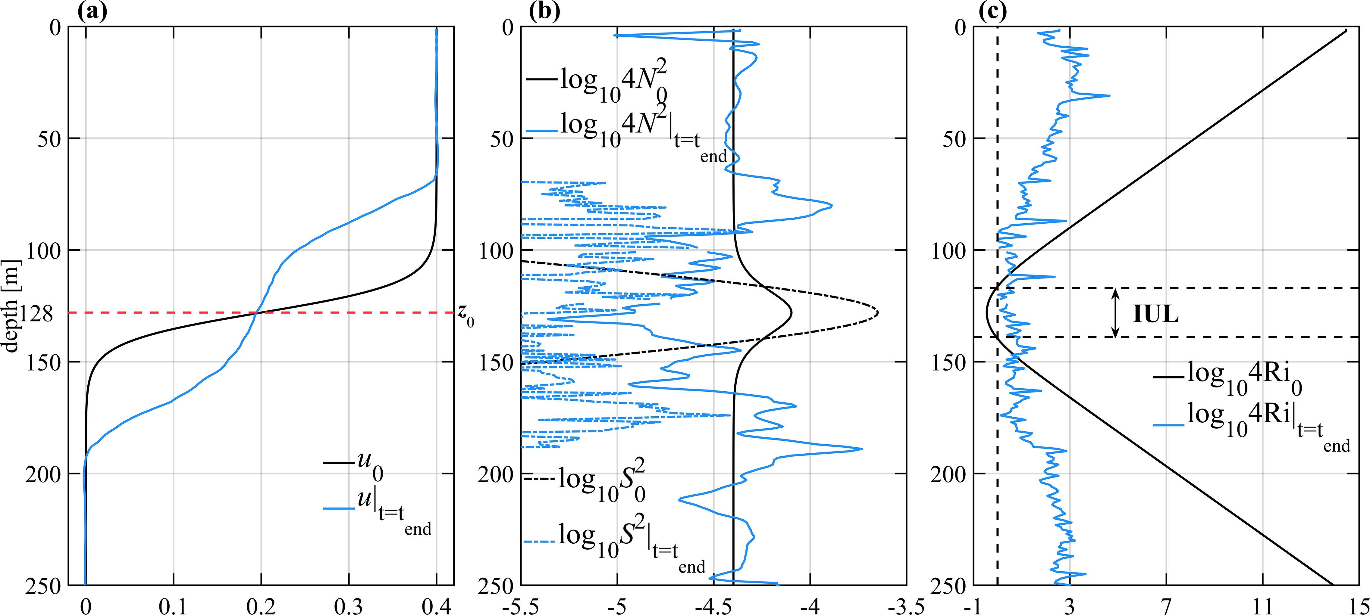
Figure 1. Initial profile and the profile at the end of the turbulent stage (t=t_end) of experiment A₇B₇ (see text). (a) Initial zonal velocity, u₀ (solid black line), and zonal velocity at the end of the turbulent stage, ${u|}_{{\text{t=t}}_{\text{end}}}$ (solid blue line) as a function of depth; the horizontal dashed red line denotes $z_0$ = 128 m. (b) The logarithmic form of four times the squared buoyancy frequency, ${\text{log}}_{10}4N_0^2$ (black solid line) and ${\text{log}}_{10}{4N}^2{|}_{{\text{t=t}}_{\text{end}}}$ (blue solid line), squared shear, ${\text{log}}_{10}{S}_0^2$ (black dot-dashed line) and ${\text{log}}_{10}{S}^2{|}_{{\text{t=t}}_{\text{end}}}$ (blue dot-dashed line). (c) The logarithmic form of four times the Richardson number, ${\text{log}}_{10}{4Ri}_0$ (black line) and ${\text{log}}_{10}{4Ri|}_{{\text{t=t}}_{\text{end}}}$ (blue line); the vertical dashed line denotes ${Ri}_0$ = 0.25, while the horizontal dashed black lines denote the upper and lower boundaries of the initial unstable layer (IUL).

$\begin{array}{ll}\begin{array}{c}{u}_0(z) = {\text{A}}_{\text{i}} \times [0.2\tanh (\frac{z + 128}{40/3}) + 0.2] (\text{m} {\text{s}}^{–1}),\end{array}& (2)\end{array}$

$\begin{array}{ll}\begin{array}{c}{N}_0^2(z) = {\text{B}}_{\text{j}} \times 0.1 \times {10}^{–4}({\mathrm{sech}}^2(\frac{z + 128}{40/3}) + 1) ({\text{s}}^{–2}).\end{array}& (3)\end{array}$

This flow structure follows that of Smyth and Peltier (1989). Here, corresponding A_i and B_j are the factors of $u_0$ and $N_0^2$, respectively. $u_0$ decreases with depth slowly above 100 m with weak shear, and decreases with depth dramatically to nearly zero at about 150 m, resulting in large shear in-between with a squared shear peak of 2.24 × 10⁻⁴ s⁻² at 128 m. $N_0^2$ has a maximum of 0.2 × 10⁻⁴ s⁻² also at 128 m; T₀ is obtained by integration of $N_0^2$ using a T-dependent ocean state equation. Consequently, the minimum of ${Ri}_0$, ${Ri}_{\min }$, reaches 0.2 at 128 m. Hereafter, the depth of 128 m is denoted as $z_0$. Away from this stratified shear layer, ${Ri}_0$ is very large: it increases from its minimum to larger than 2 above 100 m and below 150 m depths. Here, the layer with ${Ri}_0$< 0.25 is defined as the initial unstable layer (hereafter IUL). Consequently, the flow within the IUL is unstable to KH instability, which ensures the generation of turbulence after small amplitude perturbations kickstart the instability (Smyth and Peltier, 1989; Smyth et al., 2005). We note that, though these profiles cannot fully capture all potential profiles of the unstable shear layers in the ocean, they represent a large part of the characteristics of shear-driven turbulence in the stratified ocean.

A total of 27 unstable flows, with different ${Ri}_{\min }$ and IULs, have been designed to obtain sufficient turbulence properties. The parameters of the flows are listed in Table 1, where the aforementioned $u_0$ and $N_0^2$ profiles are for the experiment A₇B₇. Here we choose two other examples to depict our setting. For example, in experiment A₆B₆, the initial zonal velocity $u_0$ in A₇B₇ is multiplied by a constant factor A₆ = 0.9, which results in a $S_0^2$ that is 0.81 times that of experiment A₇B₇; at the same time, $N_0^2$ is multiplied by B₆ = 0.81, thus the ${Ri}_0$ profile of A₆B₆ remains the same as that of experiment A₇B₇. In experiment A₆B₅, the initial zonal velocity $u_0$ in A₇B₇ is multiplied by a constant factor A₆ = 0.9, but $N_0^2$ is multiplied by a constant factor B₅ = 0.64; as a result, the stratification weakens more than the shear, and the profile of ${Ri}_0$ decreases, reaching a minimum of 0.05. Based on this rule, the other 24 profiles are designed. The factors to $u_0$, named A₁–A₇, increase from 0.4 to 1.0, while the factors to $N_0^2$, named B₁–B₇, increase from 0.16 to 1.0. The set of 27 profiles contains not only variable ${Ri}_0$ (${Ri}_{\text{min}}$ ranging from 0.057 to 0.201) with constant $N_0^2$ or $S_0^2$, but also constant ${Ri}_0$ with variable $N_0^2$ or $S_0^2$, making the resulting turbulence more ergodic and the afterward statistical analysis more flexible.

Table 1

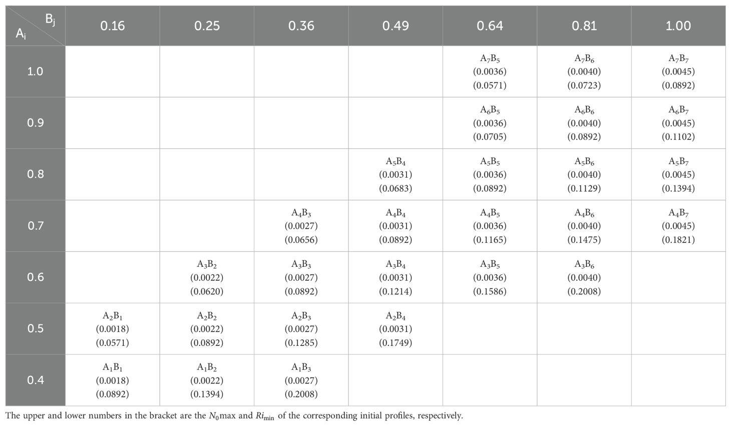
Table 1. LES experiment names, denoted as A_iB_j. Here, corresponding A_i (the first line) and B_j (the first row) are the factors of ${\text{u}}_0$ and ${\text{N}}_0^2$ expressions (Equations 2, 3), respectively.

We note that, because our study is focused on the turbulent mixing in the interior ocean, the surface forcings, including both the wind-stress-induced friction velocity and the surface heat/buoyancy flux, are set to zero in the LES experiments. This avoids the influence of boundary forcing on turbulence just below the ML base (Zaron and Moum, 2009). In addition, large-scale forcing that represents the maintenance of the background flow via larger-scale motions (Wang et al., 1998) is not set, either. As such, each of our experiments documents a non-forced evolution of turbulence, which provides ‘pure’ KH instability-induced turbulence data; this contrasts with the observed turbulence which could result from more complex processes. Due to the absence of both the external forcing and large-scale forcing, the turbulence decays rapidly which usually lasts for less than 24 hours.

2.2 Fundamental variables based on the initial conditions

Since the instability develops from the IUL, the initial variables, $\overline{N_0}$, $\overline{S_0}$ and $\overline{R{i}_0}$ are vertically averaged over the IUL. The thickness of IUL (IULT, denoted as $h_0$) is also considered an important initial variable. They are used for subsequent calculation and parameterization.

2.3 Turbulent layer and turbulent stage in the LES

2.3.1 the turbulent layer

Since a significant portion of the computational vertical layers and simulation time involves laminar flow above and below the turbulent layer, averaging turbulent statistics over the laminar regime will result in failure to accurately represent the turbulent layer properties. Smyth et al. (2005) found that the turbulent layer roughly coincided with the initial shear layer they identified, therefore they suggested that the turbulent layer can be isolated effectively from the laminar region by two isopycnic surfaces. Building on this idea, in this study, the upper and lower boundaries of the turbulent layer (hereafter TL) are defined by two surfaces, upon which the zonal velocities had the values of the upper and lower boundaries of the IUL at each moment (Figure 2).

Figure 2

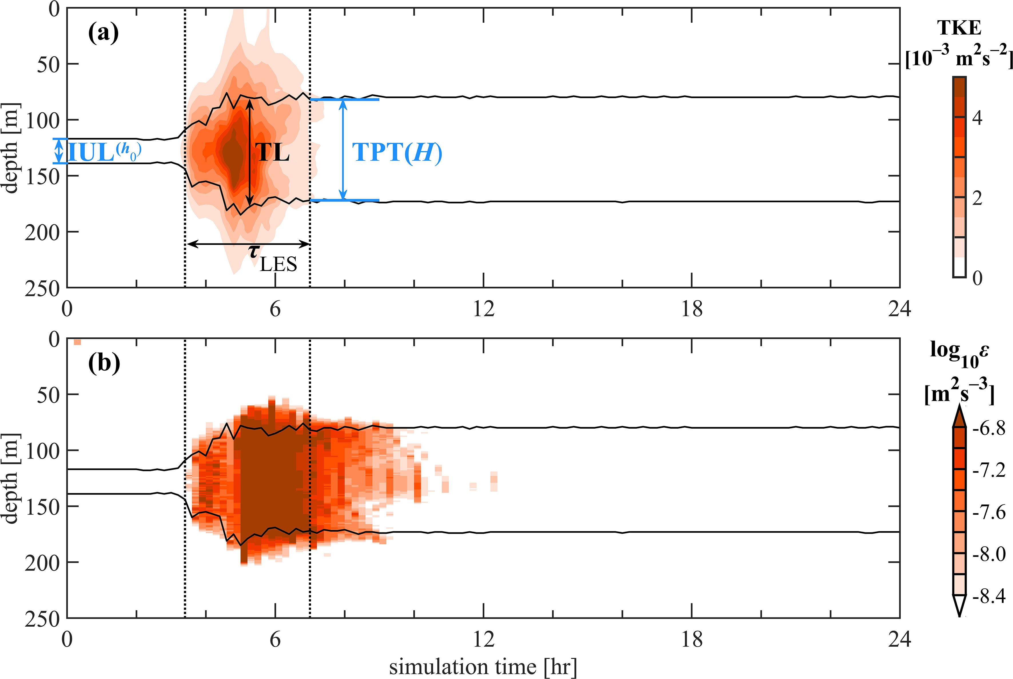
Figure 2. Time evolution of horizontal mean (a) TKE and (b) TKE dissipation rate ϵ as a function of depth for experiment A₇B₇. The Black lines denote the boundary of the turbulent layer. Horizontal blue solid lines (left) denote the upper and lower boundary of the initial unstable layer (IUL) while the horizontal blue solid lines (right) denote the upper and lower boundary of turbulent penetration, which is defined as the thickness of turbulent penetration (TPT). The vertical black dashed lines denote the start and end of the turbulent stage and the duration ${\text{τ}}_{\text{LES}}$ is defined as the difference between these 2 time nodes.

2.3.2 The turbulent stage and timescale τ_LES

A method needs to be adopted to objectively determine the turbulent stage. As for its definition, TKE is employed as a quantitative measure, because TKE is a direct measure of turbulence intensity and is also representative of turbulence generation and dissipation (Tong et al., 2022). However, using a fixed TKE threshold cannot solve the problem of the dependence of TKE on $N_0$. Here, an appropriate value of 10% of the maximum TKE over the domain and simulation time for each experiment is chosen as the threshold to identify the time range. The 2 nodes at the time axis at which the vertically averaged TKE within the TL exceeds the threshold are defined as the start and end of the turbulent stage (denoted as ${\text{t}}_{\text{start}}$ and ${\text{t}}_{\text{end}}$). The turbulent duration ${\tau }_{LES}$ is defined naturally as the difference between these 2 nodes (Figure 2). Within the turbulent duration, the TKE is firstly increased and then dissipated. Thus ${\tau }_{LES}$ can be used as the timescale of the TKE evolution. Subsequent statistical calculations are performed in the TL and turbulent stage. ${\tau }_{LES}$ is a key variable to be parameterized.

2.4 Turbulent parameters in LES

As the energy sources and sinks of turbulent evolution (Figure 3a), within the TL and over the turbulent stage, the energy transferred via shear production $E_{S{P}_{LES}}$, the energy transferred via turbulent dissipation $E_{{ϵ}_{LES}}$ and the energy transferred via buoyancy production $E_{B_{LES}}$ can be directly calculated from the LES outputs by the following equations:

Figure 3

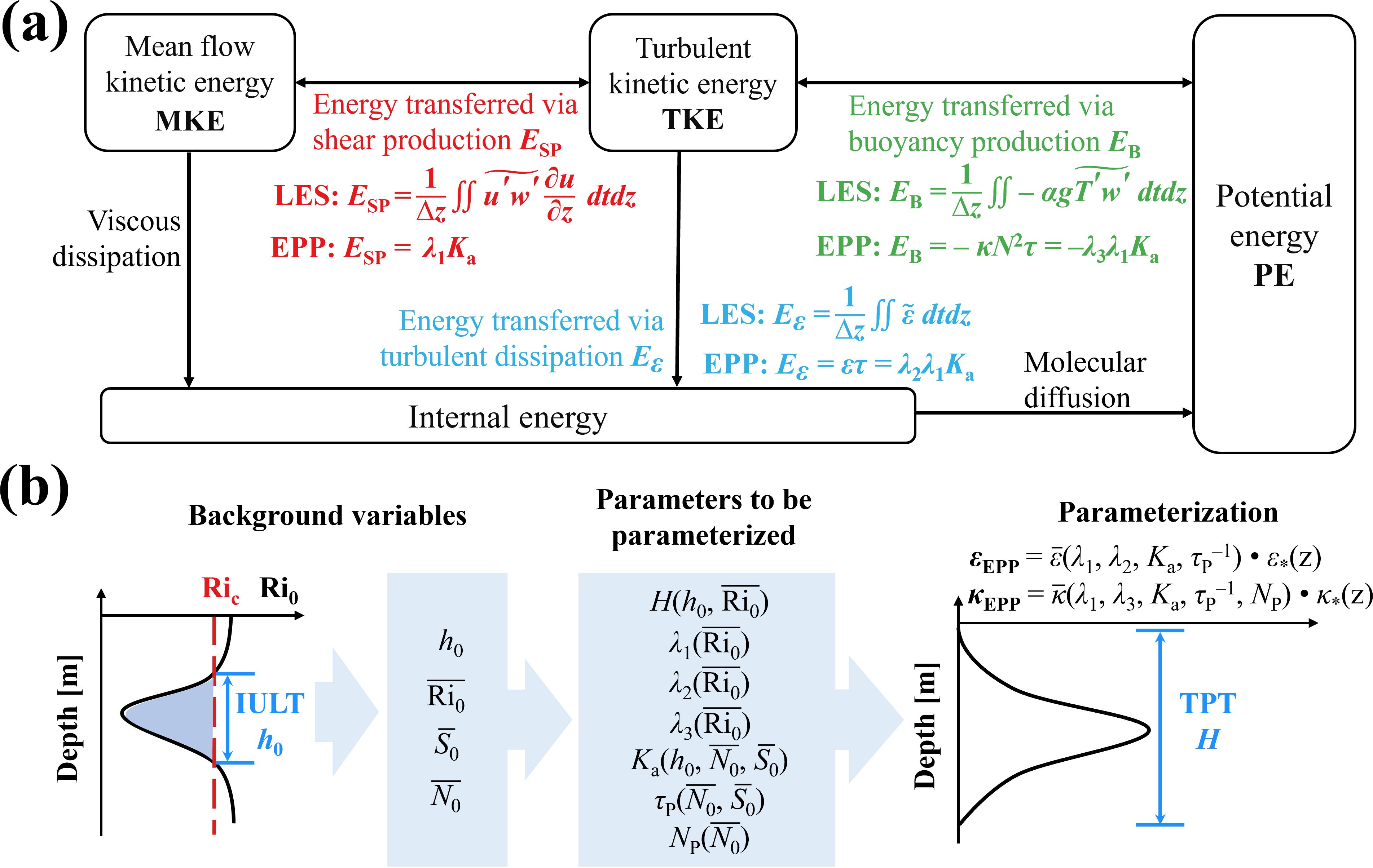
Figure 3. (a) Schematic representation of the energy transformation. Boxes represent energy reservoirs. Arrows are transfers (reversible or irreversible) between reservoirs. The transferred/transformed energy via shear production (red), turbulent dissipation (blue) and buoyancy production (green) calculated from the LES outputs and parameterized by EPP are described by (Equations 4-9). (b) Schematic of parameterization described by (Equations 10-15).

$\begin{array}{ll}{E}_{S{P}_{LES}}=\frac{1}{z_2-z_1}{\displaystyle {\int }_{z_2}^{z_2}{\displaystyle {\int }_{t=t_{start}}^{t=t_{end}}-\widetilde{u^{\prime }{w}^{\prime }}}}\frac{\partial \tilde{u}}{\partial z}\text{dt\hspace{0.17em}dz}& (4)\end{array}$

$\begin{array}{ll}{E}_{{ϵ}_{LES}}=\frac{1}{z_2-z_1}{\displaystyle {\int }_{z_1}^{z_2}{\displaystyle {\int }_{t=t_{start}}^{t=t_{end}}\widetilde{ϵ}\text{\hspace{0.17em}dt\hspace{0.17em}dz}}}& (5)\end{array}$

$\begin{array}{ll}{E}_{B_{LES}}=\frac{1}{z_2-z_1}{\displaystyle {\int }_{z_1}^{z_2}{\displaystyle {\int }_{t=t_{start}}^{t=t_{end}}-ag\widetilde{T^{\prime }{w}^{\prime }}\text{dt\hspace{0.17em}dz}}}& (6)\end{array}$

$\begin{array}{ll}{E}_{S{P}_{LES}} + E_{B_{LES}} - E_{{ϵ}_{LES}} \approx 0,& (7)\end{array}$

where ${\text{t}}_{\text{start}}$ and ${\text{t}}_{\text{end}}$ are the start and end of the turbulent stage, and z₁ and z₂ are the upper and lower boundaries of the TL. Primes and tildes represent the deviations from the horizontal mean, and the horizontal average, respectively.

The 3D (horizontally over the domain and vertically over the TL) and temporally (over the turbulent stage) averaged TKE dissipation rate ${ϵ}_{LES}$, turbulent diffusivity ${\kappa }_{LES}$ and buoyancy frequency $N_{LES}$ can be directly calculated from the LES outputs by

$${\mathit{\kappa }}_{LES}=\frac{1}{z_2-z_1}{\displaystyle {\int }_{z_1}^{z_2}-\frac{\langle \widetilde{T^{\prime }{w}^{\prime }}\rangle }{\partial \langle \tilde{T}\rangle /\partial z}}dz$$

$${ϵ}_{LES}=\frac{1}{z_2-z_1}{\displaystyle {\int }_{z_1}^{z_2}\langle \widetilde{ϵ}\rangle dz}$$

$$N_{LES}=\frac{1}{z_2-z_1}{\displaystyle {\int }_{z_1}^{z_2}\langle \tilde{N}\rangle dz}$$

where the angle brackets represent the temporal average over the turbulent stage.

In this study, the LES-provided ${ϵ}_{LES}$, ${\kappa }_{LES}$, ${\tau }_{LES}$, $N_{LES}$, $E_{S{P}_{LES}}$, $E_{{ϵ}_{LES}}$ and $E_{B_{LES}}$ will be used as the “true” values, based on which the new parameterization would be built based on the initial variables like $h_0$, $\overline{N_0}$, $\overline{S_0}$ and $\overline{R{i}_0}$ (Figure 3b).

2.5 Energy constraint framework

$E_{S{P}_{LES}}$ comes from the release of MKE, which is approximately equal to the difference in kinetic energy between the initial unstable flow and the quiescent flow after turbulence. In Figures 1b, c, at the end of the turbulent stage, the strength of shear within the TL is reduced, and the mean Ri is close to about 0.25 at the center and boundary of the TL. This indicated that the flow now reaches a marginally stable state (Thorpe and Liu, 2009).

Based on this feature, Kunze et al. (1990) assumed that the shear in an unstable stratified shear flow would be reduced if turbulent fluxes raised the $Ri = R{i}_0 < 0.25$ to $Ri = 0.25$. Assuming that shear and stratification in the IUL are constant, the difference in kinetic energy between the initial unstable state and the final state of marginal instability is defined as the AKE ($K_{\text{a}}$), and is calculated as $K_{\text{a}} = h_0^2(S^2 – 4N^2)/24$. For nonlinear shear profiles like ours, ${\text{K}}_{\text{a}}$ can be calculated as $h_0^2\overline{S_0^2 – 4N_0^2}/24$, where overbar represents the vertical average over the IUL. Though this computational approach scarifies certain physical fidelity compared to the rigorous numerical integration method, their values are consistent to a large extent (not shown); therefore, for calculation efficiency, we adopt this convenient method in the present study.

However, it is noted that the AKE ($K_{\text{a}}$) is different from $E_{S{P}_{LES}}$. $E_{S{P}_{LES}}$ represents the real released MKE throughout the TL turbulent processes, which is calculated from the LES results via (Equation 4) and is shown in Figure 3a. $K_{\text{a}}$ is proposed for the purpose of parameterization, which represents the idealized amount of MKE released through the instability, without considering the complex energetics. For this reason, let $E_{S{P}_{LES}}$ be expressed as

$\begin{array}{ll}\begin{array}{c}{E}_{S{P}_{LES}} = {\lambda }_1{K}_{\text{a}},\end{array}& (8)\end{array}$

where the parameter ${\lambda }_1$ is introduced in detail in the following framework of parameterization construction.

Furthermore, another parameter ${\lambda }_2 = E_{{ϵ}_{LES}}/E_{S{P}_{LES}}$ is introduced so that. is parameterized. Similarly, a third parameter ${\lambda }_3 = –E_{B_{LES}}/E_{S{P}_{LES}}$ is introduced. Under an assumption that the input energy is either transferred to potential energy or internal energy over the whole turbulent stage, ${\lambda }_3$ is naturally equal to $1 – {\lambda }_2$ (Figure 3a). Then, the mean $E_{{ϵ}_{LES}}$ and $E_{B_{LES}}$ can be expressed by considering the turbulent timescale ${\tau }_{LES}$ as:

$\begin{array}{ll}{E}_{{ϵ}_{LES}} = {ϵ}_{LES} · {\tau }_{LES} = {\lambda }_2{\lambda }_1{K}_{\text{a}},& \text{(9.1)}\end{array}$

$\begin{array}{ll}{E}_{B_{LES}} = {\kappa }_{LES} · N_{LES}^2 · {\tau }_{LES} = – {\lambda }_3{\lambda }_1{K}_{\text{a}}.& \text{(9.2)}\end{array}$

Here, ${\lambda }_1$, ${\lambda }_2$ and ${\lambda }_3$ are variables to be parameterized by $\overline{R{i}_0}$.

In sum, for each experiment, $K_{\text{a}}$ is calculated by initial variables, while the energy transferred via shear production ($E_{S{P}_{LES}}$) is calculated from LES outputs. By equating the parameterized $E_{S{P}_{LES}}$ to the $K_{\text{a}}$ (Equation 8), ${\lambda }_1$ is derived for each experiment. Through regression analysis, ${\lambda }_1$ is parameterized as a function of $\overline{R{i}_0}$. Similarly, parameterizations for ${\lambda }_2$, ${\lambda }_3$, $N_{LES}$ and ${\tau }_{LES}$ are obtained. Ultimately, parameterized expressions for the turbulent diffusivity and dissipation rate are derived (Figure 3b).

2.6 Observations

A dataset of observations is collected to verify our parameterization. First, turbulence activity was measured during the Tropical Instability Wave Experiment (TIWE) in the fall of 1991 at 0°, 140°W (Lien et al., 1995). During this experiment, two overlapping time series of measurements were made from two independent ships, Wecoma and Moana Wave, so the method and data can be compared and validated. 3918 casts and 2072 casts of microstructure temperature, conductivity, and shear measurements in the upper 200 m were made using the profiler CHAMELEON and the Advanced Microstructure Profiler (AMP). The horizontal velocity was measured by the ship-mounted Acoustic Doppler Current Profilers (ADCPs) with the vertical resolution of approximately 8 m.

The TKE dissipation rate ${ϵ}_{obs}$ is estimated by the method of sensing small-scale shears from the free-falling profilers (Moum et al., 1995). ${\kappa }_{obs}$ is calculated as $\gamma {ϵ}_{obs}/N^2$, where $\gamma$ is taken as a common value of 0.2 (Lien et al., 1995; Zaron and Moum, 2009). Because of the occasional necessity of repairs and delays caused by other operational difficulties, the time series of profiles was unevenly sampled. To simplify the calculation, all data were averaged hourly with the vertical resolution of 1 m. In the next subsections, we will further process this dataset to comply with our EPP scheme.

Researchers usually directly apply a parameterization to observed hydrologic data to evaluate its performance. However, we note that it is difficult to fairly evaluate the performance this way. Firstly, observational data often lack the precise background variables that are required to initialize the potential turbulent events, unlike the well-controlled initial conditions in LES experiments. The so-called background fields may also have undergone the influence of prior turbulence. Secondly, the observed mixing coefficients (such as $ϵ$ and $\kappa$) are subject to other larger-scale forces, such as advection and shear production, which is also unlike the freely developed turbulence as seen in LES. Lastly, turbulence observed at an observational site may originate from remote locations rather than local instability.

To compare EPP with observations, some turbulent events are picked out (marked by the white square in Figures 4a, b). As shown in Figures 4c, d, such turbulent events resemble LES experiments. Enhanced turbulence follows a fluid state within an IUL with $Ri \in (0, 0.25)$.

Figure 4

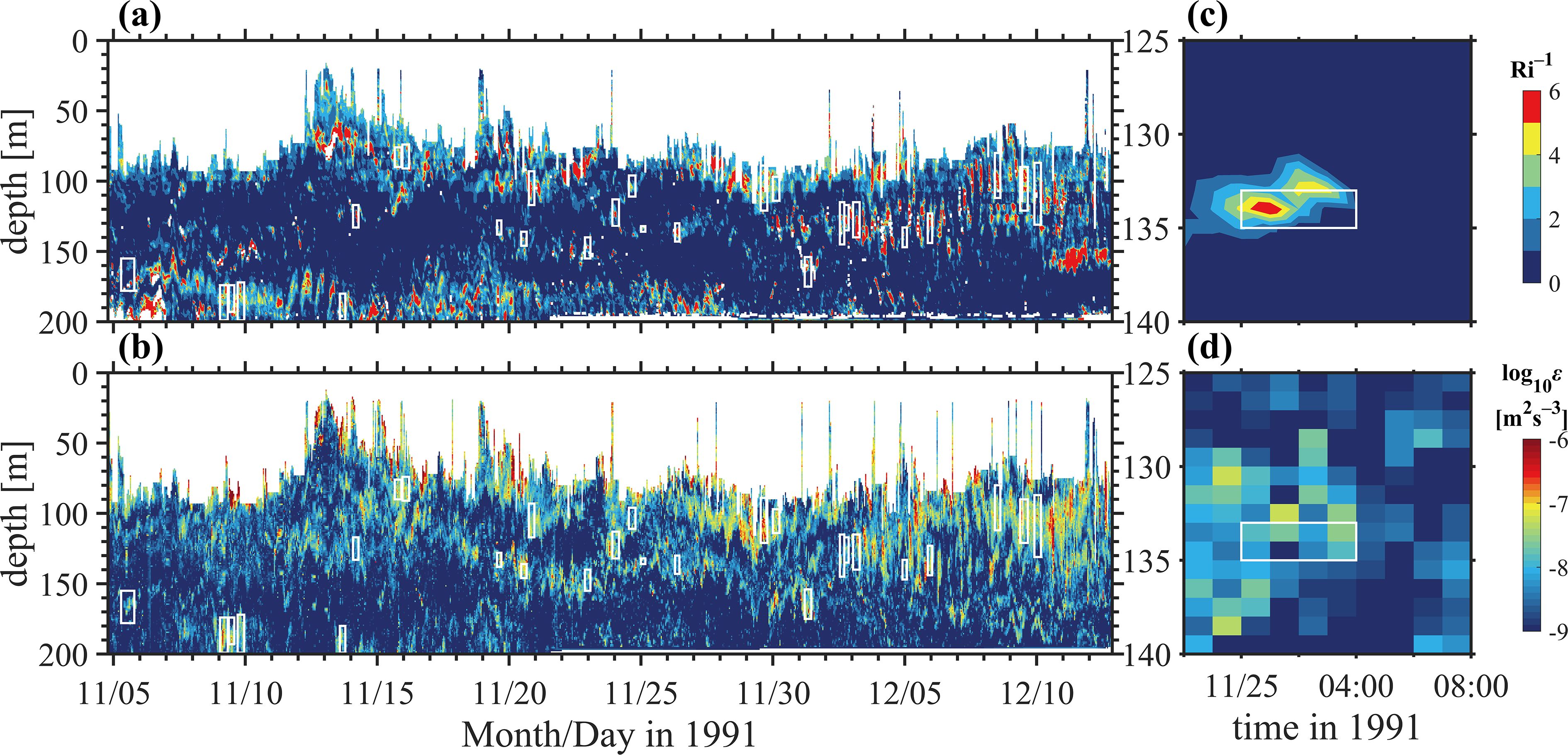
Figure 4. Depth-time plots of (a) inverse Richardson number ${Ri}^{–1}$ and (b) ϵ of TIWE. (c, d) as in (a, b) but for the turbulent events described in section 2.6. Times are UTC. White boxes represent the turbulent events. Values are blanked (white) in the ML and deep cycle layer in (a, b). The depth of ML is defined as the minimum depth within which the density is 0.01 kg m⁻³ heavier than the surface value while the DCL base is defined as the deepest depth below the ML at which Ri< 0.25 (Lien et al., 1995).

3 Turbulent properties and the parameterizations

3.1 Temporal evolution of turbulent properties: TKE, ϵ and TL

The turbulent kinetic energy (TKE) and its dissipation rate, ϵ, are important metrics describing the development and decay of turbulence. The temporal variability of horizontally averaged TKE and ϵ over each model layer, and the identified TL and turbulent stage for experiment A₇B₇ are shown in Figure 2. ${\tau }_{LES}$ is about 4 hours. TKE increases rapidly in the domain of IUL during the onset of the turbulent stage. TKE surges to a peak (~ 5 × 10⁻³ m² s⁻²) within about 1 hour in the domain of IUL. Then TKE declines gradually to the background value over 3 hours. ϵ increases and maintains a value ranging 4 × 10⁻⁹ – 4 × 10⁻⁸ m² s⁻³ during the first 2 hours of the turbulent stage. After this, ϵ surges to more than 1.6 × 10⁻⁷ m² s⁻³ and keeps for about 2 hours. Although a short period with high ϵ is excluded from the turbulent stage, most of the turbulent characteristics have been captured. ϵ for the 27 experiments show a similar evolution as described above.

In addition, due to the vertical penetration of the turbulence, the TL becomes thicker rapidly. The thickness of the TL at the end of the turbulent stage is defined as the turbulent penetration thickness (hereafter TPT, denoted as H). H (90 m) is approximately 4 times larger than $h_0$ (22 m) in experiment A₇B₇ (Figure 2). Strong vertical turbulent momentum and buoyancy fluxes therein result in a decrease in the temperature and velocity above the $z_0$ and an increase of them below the $z_0$ (Figure 1a). This variation has been shown in the direct numerical simulation results of Smyth and Winters (2003) and the CROCO ocean model results of Penney et al. (2020).

However, there is a significant difference in ${\tau }_{LES}$ across the 27 experiments, owing to the varied initial conditions (Figures 5a, b). ${\tau }_{LES}$ varies between 7920 s and 38880 s, and increases with increasing $N_0^{-1}$ which is often quoted for turbulence generation and dissipation (e.g., Moum, 1996b). Although ${\tau }_{LES}$ (i.e., 13680 s) for experiment A₇B₇ is much longer than the timescale $N_0^{-1}$ (i.e., 250 s), it is comparable with the value of Smyth et al. (2005). When $N_0$ ≈ 1 × 10⁻² s⁻¹ (their Figure 1), their duration is about 5000 s and 50 times $N_0^{-1}$. It can also be found that ${\tau }_{LES}$ appear to increase with increasing $S_0^{-1}$, which is consistent with the results of Watanabe and Nagata (2021).

Figure 5

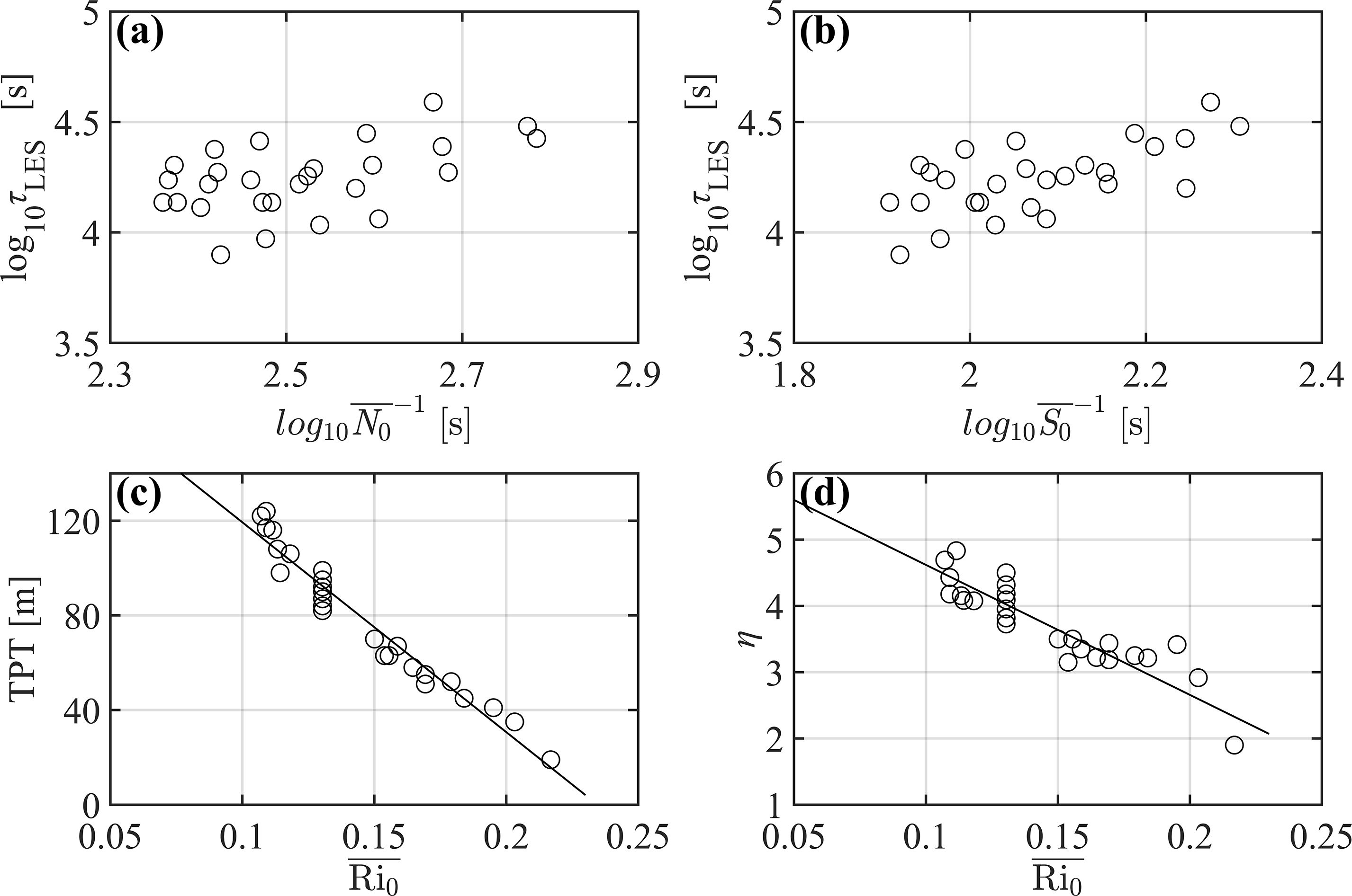
Figure 5. (a) $N_0^{–1}$ vs ${\text{τ}}_{\text{LES}}$, (b) $S_0^{–1}$ vs ${\text{τ}}_{\text{LES}}$. (c) TPT, and (d) the ratio of TPT to IULT, η, as a function of $\overline{{Ri}_0}$. The black solid lines in (c, d) denote the linearly fitted lines.

The TPTs of 27 experiments range from 20 m to 120 m, and their variations are significantly correlated with the $\overline{R{i}_0}$ (Figure 5c). A linear regression of TPT on $\overline{R{i}_0}$ can explain 96% of the variance. However, the IULT is also related to $\overline{R{i}_0}$, thus the ratio of TPT to IULT, η, is a good index representing the penetration intensity of turbulence. In Figure 5d, η is a monotone-decreasing function of $\overline{R{i}_0}$. TPTs can reach nearly 5 times the IULTs when the $\overline{R{i}_0}$ is about 0.1, which is comparable to the values of 2–3 in Smyth et al. (2005) and 5 in Penney et al. (2020). Different from the theoretical results of Kunze (2014), turbulent entrainment can also occur even for $Ri \in (0.03, 0.25)$.

3.2 Parameterization of ${ϵ}_{LES}$

To parameterize $E_{SP}$ with $K_{\text{a}}$, we calculated ${\lambda }_1$ of each experiment, and found that ${\lambda }_1$ varies between 1.5 and 25 (Figure 6a). When the velocity after simulated turbulent mixing is close to the prescribed idealized velocity of marginal instability, ${\lambda }_1$ is small and close to 1; however, the more they differ from each other, the more MKE is released and the value of ${\lambda }_1$ is larger than 1.

Figure 6

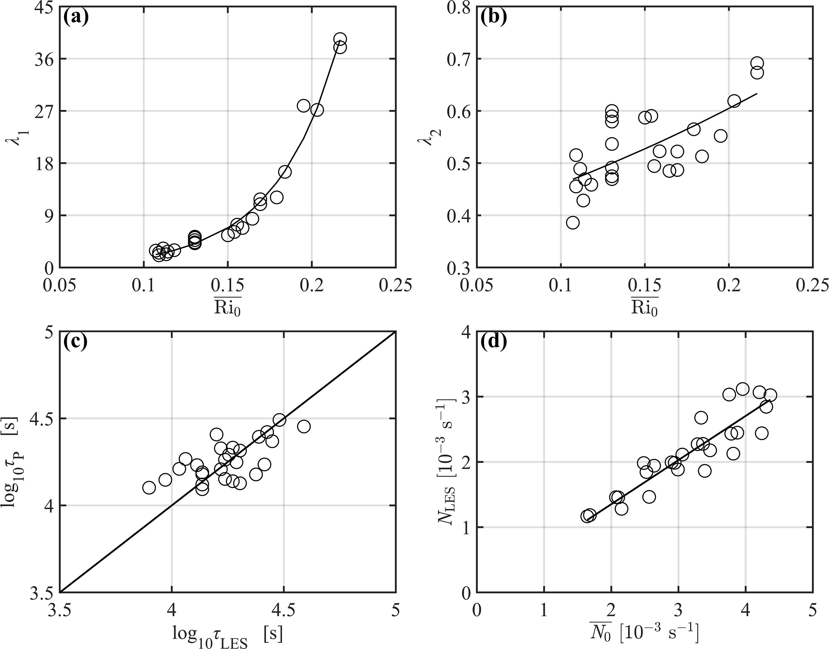
Figure 6. The ratio (a) ${\text{λ}}_1$, and (b) ${\text{λ}}_2$ as a function of $\overline{{Ri}_0}$. Comparison (c) between ${\text{τ}}_{\text{LES}}$ and ${\text{τ}}_{\text{EPP}}$, and (d) between $N_{LES}$ and $\overline{N_0}$. The black lines in (a, b, d) denote the best fits. The line in (c) denotes the 1–1 line.

Calculation based on the LES results reveals that ${\lambda }_2$ varies between 0.38 and 0.69 (Figure 6b). The larger ${\lambda }_2$ is, the larger proportion of TKE is dissipated into the internal energy. It is noted that ${\lambda }_3$ is intrinsically the flux Richardson number $R_f$, and ${\lambda }_3/{\lambda }_2$ is another measure of mixing efficiency γ which is the ratio of $–E_B$ to $E_{ϵ}$ (Smyth et al., 2001; Inoue and Smyth, 2009). We found that the values of γ range from about 0.4 to 1.4, which are larger than the commonly used value of 0.2; the underlying reason is that the calculation of γ includes the development stage of turbulence where γ is believed large (Smyth, 2020). Actually, γ can be larger than 1 when the flux Richardson number R_f is large, as seen in many numerical simulations and oceanic measurements (Moum, 1996a; Smyth et al., 2001; Salehipour and Peltier, 2015).

Finally, to parameterize $E_{SP}$, $E_{ϵ}$ and $E_B$ with $K_{\text{a}}$, ${\lambda }_1$ and ${\lambda }_2$ should be parameterized at first. We found that ${\lambda }_1$ and ${\lambda }_2$ are good functions of $\overline{R{i}_0}$ (Figures 6a, b). ${\lambda }_1$ and ${\lambda }_2$ both increase with increasing $\overline{R{i}_0}$. ${\lambda }_1$ increases exponentially with $\overline{R{i}_0}$ while ${\lambda }_2$ increases almost linearly with $\overline{R{i}_0}$. Based on the data, we give the following fitting functions,

$\begin{array}{ll}\begin{array}{c}{\lambda }_{1_P} = a{e}^{b\overline{R{i}_0}}, and {\lambda }_{2_P} = c{e}^{d\overline{R{i}_0}}.\end{array}& (10)\end{array}$

The regressions are shown in Figures 6a, b, respectively. Coefficient values and confidence intervals are listed in Table 2, and the residuals are presented in the Supplementary Material. ${\lambda }_{1_P}$ can explain about 98% of the variance of ${\lambda }_1$ (R² = 0.98), while ${\lambda }_{2_P}$ can explain about 47% of the variance of ${\lambda }_2$ (R² = 0.47). The low R² value indicates that nonlinear processes (e.g., vortex pairing) significantly modulate ${\lambda }_2$. Nevertheless, $\overline{R{i}_0}$ remains an important control parameter.

Table 2

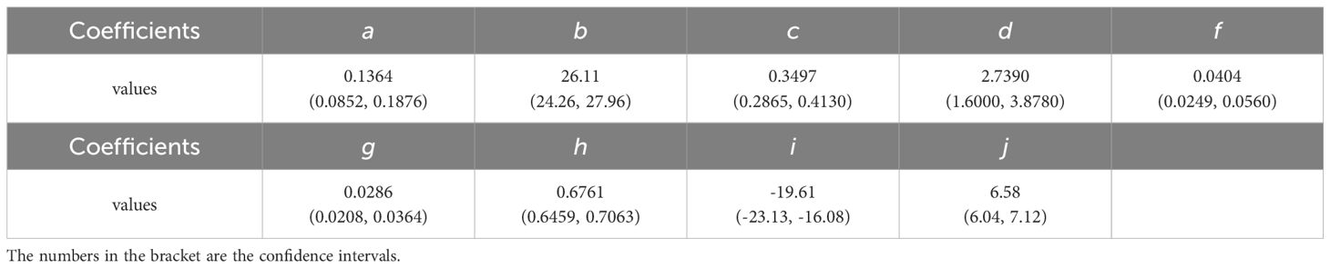
Table 2. Coefficient values of parameterizations.

In Equation 9.1, timescale ${\tau }_{LES}$ need to be parameterized. Previously, $\sigma =(S – 2N)/4$ was used by Kunze et al. (1990) to estimate the inverse timescale for the growth of small amplitude billows based on linear stability analysis (Hazel, 1972), while $N^2/S$ was used to estimate the inverse timescale for the dissipation stage after the inception of shear turbulence based on the laboratory data (Thorpe, 1973). Polzin (1996) indicated that durations for turbulent events of observations during the North Atlantic Tracer Release Experiment encompass both growth and dissipation timescales. Considering that ${\tau }_{LES}$ is the full duration of turbulent evolution, which includes both the growth and decay stages based on nonlinear numerical simulations, we parameterize the turbulent timescale ${\tau }_{LES}$ as a linear combination of the two mentioned timescales,

$\begin{array}{ll}\begin{array}{c}{\tau }_P^{ –1} = f\frac{(\overline{S_0}-2\overline{N_0})}{4} + g\frac{{\overline{N_0}}^2}{\overline{S_0}},\end{array}& (11)\end{array}$

where f and g are determined to be 0.04044 and 0.02861 by two-variable linear regression. The parameterization of ${\tau }_{LES}$, i.e., ${\tau }_P$, explains about 50% of the variance of ${\tau }_{LES}$ (R² = 0.50) as shown in Figure 6c. This expression is simple and easy to be used in the parameterization scheme. Accordingly, Equation 9.1 becomes:

$\begin{array}{ll}\begin{array}{c}{ϵ}_{EPP} = ac{e}^{(b+d)\overline{R{i}_0}} · h_0^2\frac{\overline{S_0^2-4N_0^2}}{24} · (f\frac{(\overline{S_0}-2\overline{N_0})}{4} + g\frac{{\overline{N_0}}^2}{\overline{S_0}}).\end{array}& (12)\end{array}$

Equation 12 is the energy-constrained parameterization for the TKE dissipation rate induced by the KH instability for the IUL where $Ri \in (0, 0.25)$, which is represented by the original background variables.

3.3 Parameterization of ${\kappa }_{LES}$

In the meanwhile, it is found that the stratification $N_{LES}$ in Equation 9.2 has a significant linear relationship with the initial value $\overline{N_0}$, i.e., $N_P = h\overline{N_0}$ (Figure 6d). where h is determined to be 0.6761. $N_P$ explains about 82% of the variance of $N_{LES}$ (R² = 0.82). In addition, ${\lambda }_3$ is parameterized as $1 – {\lambda }_{2_P}$. Accordingly, Equation 9.2 becomes:

$\begin{array}{ll}\begin{array}{c}{\kappa }_{EPP}=(1 c{e}^{d\overline{R{i}_0}})·a{e}^{b\overline{R{i}_0}}·h_0^2\frac{\overline{S_0^2-4N_0^2}}{24}·(f\frac{(\overline{S_0}-2\overline{N_0})}{4}+g\frac{{\overline{N_0}}^2}{\overline{S_0}})·{(h\overline{N_0})}^{ –2}.\end{array}& (13)\end{array}$

Equation 13 is the energy-constrained parameterization for κ of the KH instability-induced turbulence for the IUL where $Ri \in (0, 0.25)$, which is represented by the original background variables.

The last key property of the present parameterization lies in the vertical extension of the turbulent mixing. An important information obtained from both previous studies and the present LES results is that the shear instability-driven turbulence is not confined within the IUL, but extends to the neighboring layers. This phenomenon represents the release of accumulated energy from a potentially unstable fluid system. The TPT should represent the outer boundary of the system where the energy can be extracted. Thinking from this way, it is necessary to parameterize κ within the TPT, rather than at the grid points of $Ri \in (0, 0.25)$ only like in the previous parameterizations.

The suitable parameterization for this issue includes two steps. The first step is to identify TPT and represent it with original background variables, while the second step is to redistribute κ vertically within TPT.

Firstly, as described in section 3a, the ratio of TPT to IULT, η, varies from 2 to 5; furthermore, it can be fitted as a linear function of $\overline{R{i}_0}$ (Figure 5d)

$\begin{array}{ll}\begin{array}{c}{\eta }_P = i\overline{R{i}_0} + j,\end{array}& (14)\end{array}$

where i and j are determined as –19.61 and 6.58. ${\eta }_P$ explains about 82% of the variance of η (R² = 0.82). In practice, IULT can be determined by the grid spacing of the oceanic numerical model. Given that η can be obtained by $\overline{R{i}_0}$, the TPT can also be obtained easily, providing the layers where the parameterization should be exerted.

Secondly, the vertical distribution of κ should be provided. The previous discussion and parameterization mainly focused on the mean ${\kappa }_{LES}$ averaged vertically over the TPT under the assumption of 3D homogeneity of turbulence (Kaltenbach et al., 1994; Shih et al., 2005). Whereas, κ can be also calculated layer by layer, which can provide the vertical pattern of κ within the TL. Specifically, for each experiment, the κ profile is calculated first, and then it is normalized by ${\kappa }_{LES}$ to get ${\kappa }_{*}$, in the meanwhile, z is normalized by TPT to get $z_{*}$. Finally, the normalized profiles for 27 experiments are averaged, which is shown in Figure 7. It is found that ${\kappa }_{*}$ reaches its maximum value which is about 2 times the vertical average at the center of TPT where $R{i}_0$ is the minimum. Out of the deeper and shallower boundaries of TPT, ${\kappa }_{*}$ rapidly decreases to almost 0. Observed diffusivity profiles resulting from KH billow breakdown in the Changjiang Estuary closely match this vertical distribution (Tu et al., 2024). This pattern of normalized profile can be described by the fitting function:

Figure 7

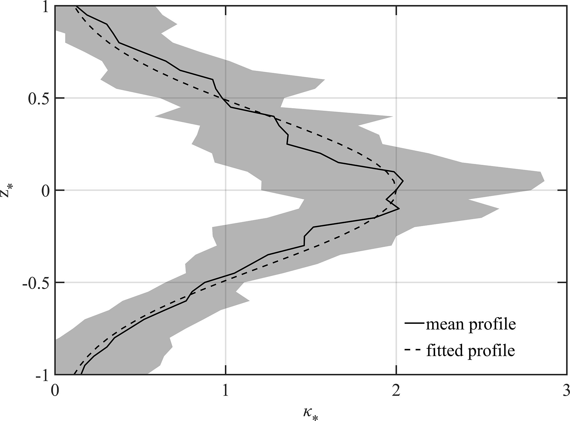
Figure 7. The mean normalized profile of ${\text{κ}}_{*}$ as a function of normalized depth ${\text{z}}_{*}$. The solid and dashed lines denote the mean and fitted profiles. Gray shading shows the standard deviation of ${\text{κ}}_{*}$ for 27 experiments.

$\begin{array}{ll}\begin{array}{c}{\kappa }_{*} = 2e^{– 1.7z_{*}^2},\end{array}& (15)\end{array}$

where $z_{*}$ represents the normalized depth of TPT. The fitted profile is very close to the actual mean profile. The profile of κ is obtained by multiplying ${\kappa }_{EPP}$ in Equation 13 by ${\kappa }_{*}$. Till now, we have finished building the new parameterization for the shear instability-driven vertical mixing in the interior ocean (Equations 13, 15).

Overall, given the new parameterization is based on an energy-constrained framework and provides the vertical diffusivity profile, it is named the energy-constrained profile parameterization, and abbreviated as EPP.

4 Comparison of the EPP with LES data, observations and existing parameterizations

In this subsection, we test the proposed EPP scheme, (Equations 12-15), against the LES data and the observations, and also compare them with existing parameterizations.

4.1 Compare ${ϵ}_{EPP}$ and ${\kappa }_{EPP}$ with LES data

It should be noted that, although the EPP schemes are based on the same set of data as ${ϵ}_{LES}$ and ${\kappa }_{LES}$, thus are non-independent, they are constructed according to the theoretical framework of energy constraint, rather than by simply fitting to ${ϵ}_{LES}$ and ${\kappa }_{LES}$. Therefore, ${ϵ}_{LES}$ and ${\kappa }_{LES}$ of LES can be used to test our scheme.

To evaluate the EPP scheme, the parameterized ${ϵ}_{EPP}$ and the original ${ϵ}_{LES}$ calculated from LES, are shown in Figure 8a. The parameterized values compare remarkably well to the values of LES. To be specific, ${ϵ}_{EPP}$ explain about 81% of the variance of ${ϵ}_{LES}$. 96% of the samples show a discrepancy within a factor of 2 for ${ϵ}_{EPP}$, while about 70% of the samples show a discrepancy only within a factor of 1.5. The parameterized diffusivity ${\kappa }_{EPP}$ and the LES-calculated diffusivity ${\kappa }_{LES}$ are compared in Figure 8b. ${\kappa }_{EPP}$ explains about 88% of the variance of ${\kappa }_{LES}$. 96% of the parameterized ${\kappa }_{EPP}$ are within a factor of 1.5 to ${\kappa }_{LES}$.

Figure 8

Figure 8. Comparison (a) between ${\text{ϵ}}_{\text{LES}}$, and ${\text{ϵ}}_{\text{EPP}}$ and ${\text{ϵ}}_{\text{RSP}}$, and (b) between ${\text{κ}}_{\text{LES}}$, and ${\text{κ}}_{\text{EPP}}$, ${\text{κ}}_{\text{RSP}}$, ${\text{κ}}_{\text{ZM}}$, ${\text{κ}}_{\text{KPP}}$, ${\text{κ}}_{\text{P}88}$ and ${\text{κ}}_{\text{PP}81}$. The lines denote the 1–1 line. Agreement within factors of 1.5 and 2 is designated by the gray bands.

Overall, the parameterized coefficients in the EPP scheme are in good agreement with the data calculated by LES, both in magnitude and variability.

4.2 Compare ${ϵ}_{EPP}$ and ${\kappa }_{EPP}$ with observations

The EPP scheme is also tested with independent observational data collected from the TIWE experiments (Lien et al., 1995). As described in section 2.6, 33 turbulent events similar to category 1 below the boundary layer (ML and deep cycle layer) are identified for the TIWE data (white squares in Figure 4).

When applying EPP to the IUL with $Ri \in (0, 0.25)$ that is below the boundary layer in observations, the TKE dissipation rate and diffusivity are calculated according to the schematic in Figure 3b. Firstly, the temperature, salinity, and velocity ${\text{u}}_0$ within the IUL can be used to calculate the initial variables, such as $\overline{N_0}$, $\overline{S_0}$ and $\overline{R{i}_0}$. Next, ${\lambda }_{1_P}$, ${\lambda }_{2_P}$, ${\lambda }_{3_P}$, $K_{\text{a}}$, ${\tau }_P$, $N_P$ and ${\eta }_P$ can be obtained with Equations 10, 11, 14. Using these variables and Equations 12, 13, the vertical average ${ϵ}_{EPP}$ and ${\kappa }_{EPP}$ are calculated. Secondly, $h_0$ is regarded as the sum of grid spacings of IUL. Multiplying ${\text{h}}_0$ by the ratio ${\eta }_P$, the TPT and grids within which the turbulence can penetrate are obtained. Finally, by multiplying ${\kappa }_{EPP}$ by the normalized profile from Equation 15, the ${\kappa }_{EPP}$ profile is obtained. It is worth noting that, possibly due to the influence of other forcings, the stratification within turbulent events is not always smaller than the initial value $\overline{N_0}$ as in LES. Therefore, we use the observed buoyancy frequency as $N_P$.

Applying the EPP to the 33 turbulent events, it is seen that the parameterized values can basically capture the magnitude and amplitude of the observed ${ϵ}_{obs}$ and ${\kappa }_{obs}$ (Figure 9). The agreements between ${ϵ}_{EPP}$ and ${ϵ}_{obs}$, and between ${\kappa }_{EPP}$ and ${\kappa }_{obs}$ are both within a factor of 10 for about 88% and a factor of 5 for about 70%, respectively. Nonetheless, the EPP shows advantages compared to the widely used previous schemes, which is discussed in the next subsection.

Figure 9

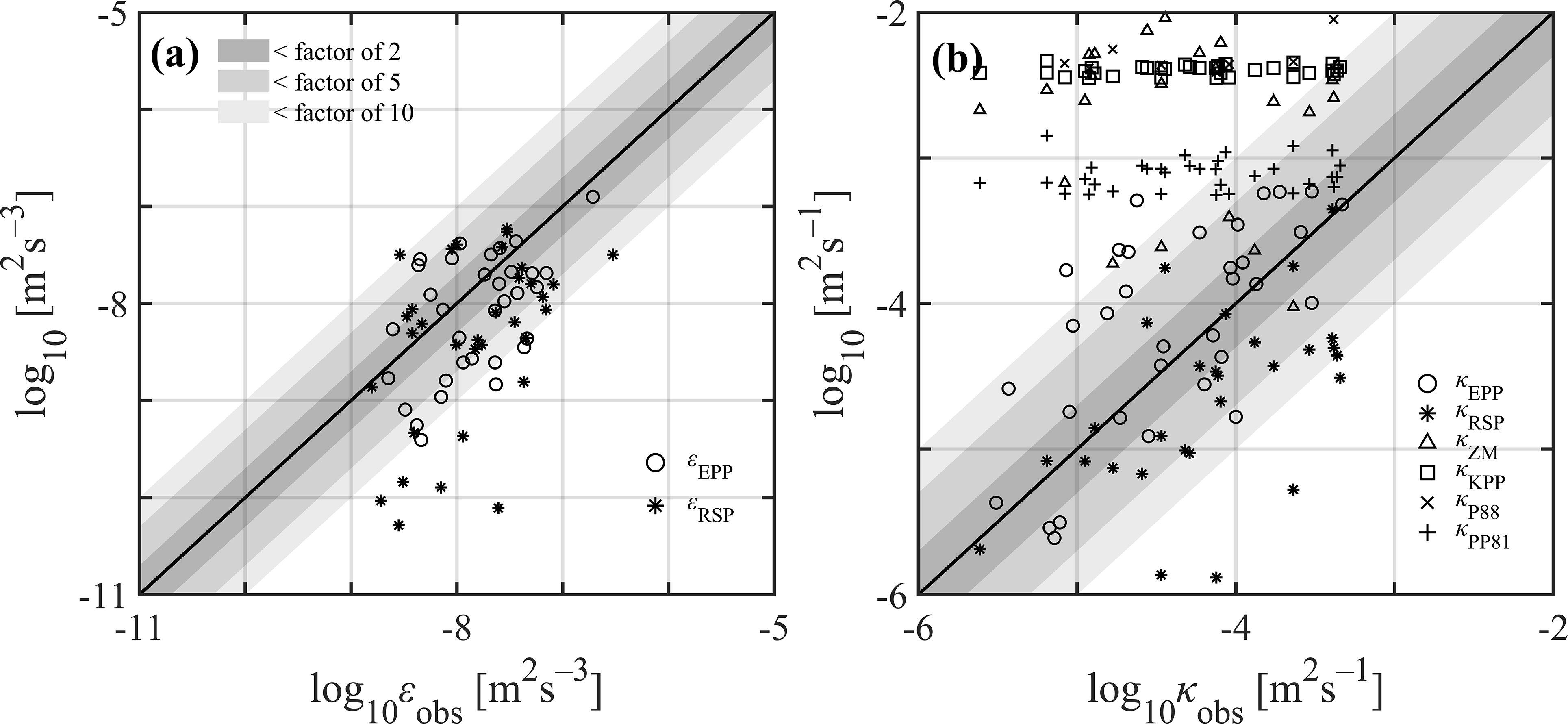
Figure 9. Comparison (a) between ${\text{ϵ}}_{\text{obs}}$ and ${\text{ϵ}}_{\text{EPP}}$, and (b) between ${\text{κ}}_{\text{obs}}$, and ${\text{κ}}_{\text{EPP}}$, ${\text{κ}}_{\text{RSP}}$, ${\text{κ}}_{\text{ZM}}$, ${\text{κ}}_{\text{KPP}}$, ${\text{κ}}_{\text{P}88}$ and ${\text{κ}}_{\text{PP}81}$.

4.3 Compare ${ϵ}_{EPP}$ and ${\kappa }_{EPP}$ with previous schemes

Several previous parameterizations, including RSP, ZM (Zaron and Moum, 2009), PP81, P88 and KPP are compared, which shows an overall better performance of EPP. REV parameterization is used for ZM while shear instability mixing component of KPP is adopted for comparison. Through the comparison, we also analyze the underlying mechanisms why EPP performs better.

As shown in Figure 8a, if taking the LES as metrics, ${ϵ}_{RSP}$ overestimates ${ϵ}_{LES}$, and has a larger scatter than ${ϵ}_{EPP}$, while only 59.3% of ${\kappa }_{RSP}$ are within a factor of 2, compared to the 100% of ${ϵ}_{EPP}$. This may be due to the large inverse timescale employed in the RSP scheme, which results in a large ${ϵ}_{RSP}$, but its smaller γ partially offsets this overestimation. ${\kappa }_{KPP}$, ${\kappa }_{PP81}$ and ${\kappa }_{ZM}$ all underestimate the ${\kappa }_{LES}$ by a factor of 4–18 on average, while ${\kappa }_{P88}$ overestimates them by a factor of 18. KPP, PP81, and ZM all prescribe distinct yet nearly invariant diffusivity when the Ri< 0.25 based on observed averages. Their empirical rigidity neglecting turbulence-scale dynamics in idealized LES experiments. For P88, the overestimation stems from its mathematical formulation where ${\kappa }_{P88}$ tends toward infinity as Ri approaches 0. The EPP seems to best fit the data, this is because this scheme fully considers the dynamical variables in addition to $\overline{R{i}_0}$.

As for the parameterizations of the observations (Figure 9a), more of ${ϵ}_{RSP}$ underestimates ${ϵ}_{obs}$ than ${ϵ}_{EPP}$, but about 72% of ${ϵ}_{RSP}$ approximate ${ϵ}_{obs}$ well. 73% of the parameterized ${\kappa }_{RSP}$ are within a factor of 10, while 58% of the samples are within a factor of 5. Compared with ${ϵ}_{EPP}$, more of ${\kappa }_{RSP}$ underestimate ${\kappa }_{obs}$. ${\kappa }_{ZM}$, ${\kappa }_{KPP}$, ${\kappa }_{PP81}$ and ${\kappa }_{P88}$ overestimate ${\kappa }_{obs}$ by more than a factor of 10 on average, and they fail to capture the variability of ${\kappa }_{obs}$. The fact that variability of turbulent diffusivity depends not only on ${Ri}_0$ but also on other variables such as shear and stratification (Richards et al., 2021) is obviously missed in these parametrizations. ${\kappa }_{KPP}$ and ${\kappa }_{PP81}$ overestimate ${\kappa }_{obs}$, indicating that KPP and PP81 must adjust their parameters according to the observations at different conditions to achieve the best parameterization, but it is almost impossible to experience all different conditions. In contrast, the EPP and RSP is relatively adaptive to the observations and LES data.

5 Summary and discussion

Shear-driven turbulence in the interior stratified shear flow is an important process in the ocean, but it is difficult to measure and simulate in ocean models. The existing parameterizations for turbulent diffusivity are usually based on the background gradient Richardson number only, which is not sufficient to capture the strength and variability of turbulence intensity.

For shear-driven turbulence in the internal ocean with $Ri\in (0, 0.25)$, we present a new energy-constrained profile parameterization, EPP. The parameterization includes both the TKE dissipation rate ϵ and the diffusivity $\kappa$. EPP is based on an energy-constrained framework, which assumes that the TKE dissipation rate ϵ is proportional to both the available kinetic energy $K_{\text{a}}$ and the inversed turbulent timescale ${\tau }_{LES}^{–1}$. $K_{\text{a}}$ is defined as the difference between the initial kinetic energy of the unstable flow and the kinetic energy of the corresponding idealized marginally stable flow. ${\tau }_{LES}$ is a function of both the background buoyancy frequency $\overline{N_0}$ and shear $\overline{S_0}$. The parameterization also includes 2 factors, ${\lambda }_{1_P}$ and ${\lambda }_{2_P}$, both of which depend on $R{i}_0$, and denote the ratio of the energy transferred via shear production $E_{S{P}_{LES}}$ to $K_{\text{a}}$, and the ratio of the energy transferred via turbulent dissipation $E_{{ϵ}_{LES}}$ to $E_{S{P}_{LES}}$, respectively. Similarly, introducing the ratio of the energy transferred via buoyancy production $E_{B_{LES}}$ to $E_{{\text{SP}}_{\text{LES}}}$, the corresponding vertical diffusivity $\kappa$ is also parameterized by the variables mentioned above (Equation 13).

Such turbulence events are observed under the surface boundary layer, such as subsurface turbulent mixing in the eastern equatorial Pacific and western boundary currents. Jia et al. (2021) suggested that a high vertical resolution model can capture many characteristics of small-scale velocity and density in the upper ocean. A lot of unstable flows of $\text{Ri }\in \text{ (0, 0}\mathrm{.25)}$ can be simulated in future numerical models with much higher vertical resolution than now. The increased shear-driven turbulent mixing is expected to be reasonably represented by this new parameterization. However, the transferability of EPP to larger-scale or more complex oceanic environments remains constrained by two key limitations: (1) The omission of rotational effects, which may distort energy cascades in mid-latitude western boundary currents; (2) Its calibration against limited-depth LES (≤ 256 m), potentially restricting its capacity to adequately capture deep-ocean processes such as mixing driven by internal wave breaking. Future iterations need incorporate rotational terms and extend validation to the full water column.

Furthermore, because the shear-driven turbulence can penetrate vertically from the layer of the low Ri to a thick surrounding layer, the thickness of which is denoted as TPT. The TPT could be several times the IULT, and may exceed several grid spacings in the numerical model. Thus, we propose a method to parameterize TPT according to initial variables, and hence construct a function of the normalized profile ${\text{κ}}_{*}$ within the TPT. Introducing TPT in the EPP scheme is certainly a step forward in improving the simulation of turbulent mixing on adjacent layers. This means that the turbulent mixing may provide an additional independent factor affecting the surrounding environment; the effect on the temperature/salinity change to the neighboring grid could be large or small, depending on whether it dominates other terms. The parameterization is calibrated using LES and tested using equatorial observations. The results show that the new parameterization can capture the variability and magnitude of turbulence, and performs better than widely-used parameterizations. Given that RSP and EPP are both based on the energy constraint framework, RSP can serve as a viable alternative to EPP. The concise formulation of RSP enables high computational efficiency. Specifically, the diffusivity derived from RSP can be combined with the diffusivity profile function of the EPP scheme. This hybrid scheme provides a practical and efficient alternative to the original EPP. The application of this parameterization in a high-resolution numerical model will be reported later.

Data availability statement

The datasets presented in this study can be found in online repositories. The names of the repository/repositories and accession number(s) can be found below: https://doi.org/10.5281/zenodo.15064783 and https://microstructure.ucsd.edu/#/cruise/32WC19911104.

Author contributions

LL: Data curation, Writing – original draft, Investigation. CL: Writing – review & editing, Conceptualization. RH: Writing – review & editing. FW: Funding acquisition, Writing – review & editing.

Funding

The author(s) declare that financial support was received for the research and/or publication of this article. This study is supported by National Natural Science Foundation of China (42090040), National Natural Science Foundation of China (42430403), the Key Research Program of Laoshan Laboratory (LSL) (2022LSL010302), and the National Key R&D Program of China (2022YFF0801404).

Acknowledgments

The authors would like to thank two anonymous reviewers for providing insightful comments. We acknowledge the technical support from Oceanographic Data Center, IOCAS.We acknowledge the TIWE team that contributed to the collection of the TIWE microstructure data.

Conflict of interest

The authors declare that the research was conducted in the absence of any commercial or financial relationships that could be construed as a potential conflict of interest.

Generative AI statement

The author(s) declare that no Generative AI was used in the creation of this manuscript.

Any alternative text (alt text) provided alongside figures in this article has been generated by Frontiers with the support of artificial intelligence and reasonable efforts have been made to ensure accuracy, including review by the authors wherever possible. If you identify any issues, please contact us.

Publisher’s note

All claims expressed in this article are solely those of the authors and do not necessarily represent those of their affiliated organizations, or those of the publisher, the editors and the reviewers. Any product that may be evaluated in this article, or claim that may be made by its manufacturer, is not guaranteed or endorsed by the publisher.

Supplementary material

The Supplementary Material for this article can be found online at: https://www.frontiersin.org/articles/10.3389/fmars.2025.1615741/full#supplementary-material

References

Chang Y. S., Xu X., Özgökmen T. M., Chassignet E. P., Peters H., and Fischer P. F. (2005). Comparison of gravity current mixing parameterizations and calibration using a high-resolution 3D nonhydrostatic spectral element model. Ocean Model. 10, 342–368. doi: 10.1016/j.ocemod.2004.11.002

Crossref Full Text | Google Scholar

Geyer W. R., Lavery A. C., Scully M. E., and Trowbridge J. H. (2010). Mixing by shear instability at high Reynolds number. Geophysical Res. Lett. 37. doi: 10.1029/2010gl045272

Crossref Full Text | Google Scholar

Hazel P. (1972). Numerical studies of the stability of inviscid stratified shear flows. J. Fluid Mechanics 51, 39–61. doi: 10.1017/s0022112072001065

Crossref Full Text | Google Scholar

Howard L. N. (1961). Note on a paper of john W. Miles. J. Fluid Mechanics 10, 509–512. doi: 10.1017/S0022112061000317

Crossref Full Text | Google Scholar

Inoue R., Lien R.-C., and Moum J. N. (2012). Modulation of equatorial turbulence by a tropical instability wave. J. Geophysical Research: Oceans 117. doi: 10.1029/2011jc007767

Crossref Full Text | Google Scholar

Inoue R. and Smyth W. D. (2009). Efficiency of mixing forced by unsteady shear flow. J. Phys. Oceanography 39, 1150–1166. doi: 10.1175/2008jpo3927.1

Crossref Full Text | Google Scholar

Jia Y., Richards K. J., and Annamalai H. (2021). The impact of vertical resolution in reducing biases in sea surface temperature in a tropical Pacific Ocean model. Ocean Model. 157, 101722. doi: 10.1016/j.ocemod.2020.101722

Crossref Full Text | Google Scholar

Kaltenbach H.-J., Gerz T., and Schumann U. (1994). Large-eddy simulation of homogeneous turbulence and diffusion in stably stratified shear flow. J. Fluid Mechanics 280, 1–40. doi: 10.1017/s0022112094002831

Crossref Full Text | Google Scholar

Klemp J. B. and Durran D. R. (1983). An upper boundary condition permitting internal gravity wave radiation in numerical mesoscale models. Monthly Weather Rev. 111, 430–444. doi: 10.1175/1520-0493(1983)111<0430:Aubcpi>2.0.Co;2

Crossref Full Text | Google Scholar

Kunze E. (2014). The relation between unstable shear layer thicknesses and turbulence lengthscales. J. Mar. Res. 72, 95–104. doi: 10.1357/002224014813758977

Crossref Full Text | Google Scholar

Kunze E., Williams A. J., and Briscoe M. G. (1990). Observations of shear and vertical stability from a neutrally buoyant float. J. Geophysical Res. 95, 18127. doi: 10.1029/jc095ic10p18127

Crossref Full Text | Google Scholar

Large W. G., Mcwilliams J. C., and Doney S. C. (1994). Oceanic vertical mixing: A review and a model with a nonlocal boundary layer parameterization. Rev. Geophysics 32, 363. doi: 10.1029/94rg01872

Crossref Full Text | Google Scholar

Lien R.-C., Caldwell D. R., Gregg M. C., and Moum J. N. (1995). Turbulence variability at the equator in the central Pacific at the beginning of the 1991–1993 El Niño. J. Geophysical Res. 100, 6881. doi: 10.1029/94jc03312

Crossref Full Text | Google Scholar

Miles J. W. (1961). On the stability of heterogeneous shear flows. J. Fluid Mechanics 10, 496–508. doi: 10.1017/S0022112061000305

Crossref Full Text | Google Scholar

Moeng C.-H. (1984). A large-eddy-simulation model for the study of planetary boundary-layer turbulence. J. Atmospheric Sci. 41, 2052–2062. doi: 10.1175/1520-0469(1984)041<2052:Alesmf>2.0.Co;2

Crossref Full Text | Google Scholar

Moum J. N. (1996a). Efficiency of mixing in the main thermocline. J. Geophysical Research: Oceans 101, 12057–12069. doi: 10.1029/96jc00508

Crossref Full Text | Google Scholar

Moum J. N. (1996b). Energy-containing scales of turbulence in the ocean thermocline. J. Geophysical Research: Oceans 101, 14095–14109. doi: 10.1029/96jc00507

Crossref Full Text | Google Scholar

Moum J. N., Gregg M. C., Lien R. C., and Carr M. E. (1995). Comparison of turbulence kinetic energy dissipation rate estimates from two ocean microstructure profilers. J. Atmospheric Oceanic Technol. 12, 346–366. doi: 10.1175/1520-0426(1995)012<0346:COTKED>2.0.CO;2

Crossref Full Text | Google Scholar

Moum J. N., Hebert D., Paulson C. A., and Caldwell D. R. (1992). Turbulence and internal waves at the equator. Part I: statistics from towed thermistors and a microstructure profiler. J. Phys. Oceanography 22, 1330–1345. doi: 10.1175/1520-0485(1992)022<1330:taiwat>2.0.co;2

Crossref Full Text | Google Scholar

Osborn T. R. (1980). Estimates of the local rate of vertical diffusion from dissipation measurements. J. Phys. Oceanography 10, 83–89. doi: 10.1175/1520-0485(1980)010<0083:Eotlro>2.0.Co;2

Crossref Full Text | Google Scholar

Pacanowski R. C. and Philander S. G. H. (1981). Parameterization of vertical mixing in numerical models of tropical oceans. J. Phys. Oceanography 11, 1443–1451. doi: 10.1175/1520-0485(1981)011<1443:Povmin>2.0.Co;2

Crossref Full Text | Google Scholar

Penney J., Morel Y., Haynes P., Auclair F., and Nguyen C. (2020). Diapycnal mixing of passive tracers by Kelvin–Helmholtz instabilities. J. Fluid Mechanics 900. doi: 10.1017/jfm.2020.483

Crossref Full Text | Google Scholar

Peters H., Gregg M. C., and Toole J. M. (1988). On the parameterization of equatorial turbulence. J. Geophysical Res. 93, 1199. doi: 10.1029/jc093ic02p01199

Crossref Full Text | Google Scholar

Pham H. T. and Sarkar S. (2022). A comparative study of turbulent stratified shear layers: effect of density gradient distribution. Environ. Fluid Mechanics. doi: 10.1007/s10652-022-09873-2

Crossref Full Text | Google Scholar

Pham H. T., Sarkar S., Smyth W. D., Moum J. N., and Warner S. J. (2024). Deep-cycle turbulence in the upper pacific equatorial ocean: characterization by LES and heat flux parameterization. J. Phys. Oceanography 54, 577–599. doi: 10.1175/JPO-D-23-0015.1

Crossref Full Text | Google Scholar

Polzin K. (1996). Statistics of the richardson number: mixing models and finestructure. J. Phys. Oceanography 26, 1409–1425. doi: 10.1175/1520-0485(1996)026<1409:SOTRNM>2.0.CO;2

Crossref Full Text | Google Scholar

Richards K. J., Natarov A., and Carter G. S. (2021). Scaling of shear-generated turbulence: the equatorial thermocline, a case study. J. Geophysical Research: Oceans 126. doi: 10.1029/2020jc016978

Crossref Full Text | Google Scholar

Salehipour H. and Peltier R. (2015). Diapycnal diffusivity, turbulent Prandtl number and mixing efficiency in Boussinesq stratified turbulence. J. Fluid Mechanics 775, 464–500. doi: 10.1017/jfm.2015.305

Crossref Full Text | Google Scholar

Shih L. H., Koseff J. R., Ivey G. N., and Ferziger J. H. (2005). Parameterization of turbulent fluxes and scales using homogeneous sheared stably stratified turbulence simulations. J. Fluid Mechanics 525, 193–214. doi: 10.1017/s0022112004002587

PubMed Abstract | Crossref Full Text | Google Scholar

Smyth W. D. (2020). Marginal instability and the efficiency of ocean mixing. J. Phys. Oceanography 50, 2141–2150. doi: 10.1175/jpo-d-20-0083.1

Crossref Full Text | Google Scholar

Smyth W. D., Carpenter J. R., and Lawrence G. A. (2007). Mixing in symmetric holmboe waves. J. Phys. Oceanography 37, 1566–1583. doi: 10.1175/jpo3037.1

Crossref Full Text | Google Scholar

Smyth W. D. and Moum J. N. (2012). Ocean mixing by kelvin-helmholtz instability. Oceanography 25, 140–149. doi: 10.5670/oceanog.2012.49

Crossref Full Text | Google Scholar

Smyth W. D., Moum J. N., and Caldwell D. R. (2001). The efficiency of mixing in turbulent patches: inferences from direct simulations and microstructure observations. J. Phys. Oceanography 31, 1969–1992. doi: 10.1175/1520-0485(2001)031<1969:teomit>2.0.co;2

Crossref Full Text | Google Scholar

Smyth W. D., Nash J. D., and Moum J. N. (2005). Differential diffusion in breaking kelvin–helmholtz billows. J. Phys. Oceanography 35, 1004–1022. doi: 10.1175/jpo2739.1

Crossref Full Text | Google Scholar

Smyth W. D. and Peltier W. R. (1989). The transition between kelvin–helmholtz and holmboe instability: an investigation of the overreflection hypothesis. J. Atmospheric Sci. 46, 3698–3720. doi: 10.1175/1520-0469(1989)046<3698:ttbkah>2.0.co;2

Crossref Full Text | Google Scholar

Smyth W. D. and Winters K. B. (2003). Turbulence and mixing in holmboe waves. J. Phys. Oceanography 33, 694–711. doi: 10.1175/1520-0485(2003)33<694:Tamihw>2.0.Co;2

Crossref Full Text | Google Scholar

Sullivan P., Mcwilliams J., and Moeng C. (1996). A grid nesting method for large-eddy simulation of planetary boundary layer flows. Boundary Layer Meteorology 80, 167–202. doi: 10.1007/BF00119016

Crossref Full Text | Google Scholar

Thorpe S. A. (1973). Experiments on instability and turbulence in a stratified shear flow. J. Fluid Mechanics 61, 731–751. doi: 10.1017/s0022112073000911

Crossref Full Text | Google Scholar

Thorpe S. A. and Liu Z. (2009). Marginal instability? J. Phys. Oceanography 39, 2373–2381. doi: 10.1175/2009jpo4153.1

Crossref Full Text | Google Scholar

Tong B., Guo J., Wang Y., Li J., Yun Y., Solanki R., et al. (2022). The near-surface turbulent kinetic energy characteristics under the different convection regimes at four towers with contrasting underlying surfaces. Atmospheric Res. 270, 106073. doi: 10.1016/j.atmosres.2022.106073

Crossref Full Text | Google Scholar

Tu J., Wu J., Fan D., Liu Z., Zhang Q., and Smyth W. (2024). Shear instability and turbulent mixing by kuroshio intrusion into the changjiang river plume. Geophysical Res. Lett. 51. doi: 10.1029/2024gl110957

Crossref Full Text | Google Scholar

Wang D., Large W. G., and McWilliams J. C. (1996). Large-eddy simulation of the equatorial ocean boundary layer: Diurnal cycling, eddy viscosity, and horizontal rotation. J. Geophysical Research: Oceans 101, 3649–3662. doi: 10.1029/95jc03441

Crossref Full Text | Google Scholar

Wang D., McWilliams J. C., and Large W. G. (1998). Large-eddy simulation of the diurnal cycle of deep equatorial turbulence. J. Phys. Oceanography 28, 129–148. doi: 10.1175/1520-0485(1998)028<0129:Lesotd>2.0.Co;2

Crossref Full Text | Google Scholar

Wang D. and Müller P. (2002). Effects of equatorial undercurrent shear on upper-ocean mixing and internal waves. J. Phys. Oceanography 32, 1041–1057. doi: 10.1175/1520-0485(2002)032<1041:Eoeuso>2.0.Co;2

Crossref Full Text | Google Scholar

Watanabe T. and Nagata K. (2021). Large-scale characteristics of a stably stratified turbulent shear layer. J. Fluid Mechanics 927. doi: 10.1017/jfm.2021.773

Crossref Full Text | Google Scholar

Winters K. B., Lombard P. N., Riley J. J., and D'Asaro E. A. (1995). Available potential energy and mixing in density-stratified fluids. J. Fluid Mechanics 289, 115–128. doi: 10.1017/s002211209500125x

Crossref Full Text | Google Scholar

Zaron E. D. and Moum J. N. (2009). A new look at richardson number mixing schemes for equatorial ocean modeling. J. Phys. Oceanography 39, 2652–2664. doi: 10.1175/2009jpo4133.1

Crossref Full Text | Google Scholar