Seasonal air-sea CO2 flux dynamics in Colombia’s Gorgona Marine Area during La Niña 2021–2022

Air–sea CO₂ fluxes in tropical coastal zones are strongly influenced by ENSO variability, but in situ measurements in the Eastern Tropical Pacific remain scarce. We assessed seasonal CO₂ dynamics around Gorgona Island (Panama Bight, Colombian Pacific) under La Niña 2021–2022. From November 2021 to July 2022, we conducted monthly sampling at seven stations spanning the Guapi River plume to the open ocean, measuring physical (SST, SSS, thermocline depth), chemical (TA, DIC, pH, carbonate system parameters), and biological (chlorophyll-a) variables, and estimating net CO₂ fluxes (FCO₂) with the Liss and Merlivat (1986) parameterization and atmospheric CO₂ from NOAA. La Niña featured a cool-water anomaly (−0.78 °C), enhanced precipitation (+59%) and river discharge (+44%) relative to multi-year means. The nine-month mean CO₂ flux was near neutral (−0.01049 ± 0.00014 mol C m⁻²) but strongly seasonal: six post-upwelling months showed slightly positive fluxes (0.00929 ± 0.000147 mol C m⁻²) associated with high precipitation (746.4 ± 214.7 mm), warmer SST (27.5 ± 0.4 °C), elevated pCO₂w (567 ± 97.5 µatm) and lower pH (7.869 ± 0.040), whereas three upwelling months showed slightly negative fluxes (−0.00119 ± 0.00010 mol C m⁻²) with reduced precipitation (165.8 ± 82.4 mm), cooler SST (26.5 ± 0.2 °C), lower pCO₂w (461 ± 92.8 µatm) and higher pH (7.968 ± 0.048). La Niña amplified pCO₂w variability (316–839 µatm) via vertical Ekman pumping, horizontal transport (Zonal Ekman Transport, tides), and freshwater inputs, while a persistent thermocline (10–40.1 m) restricted deep CO₂-rich waters from reaching the surface. Biological uptake further modulated outgassing, as evidenced by chlorophyll-a and ΔDIC dynamics. Overall, CO₂ fluxes were relatively low compared with other tropical estuarine and oceanic sources. These results underscore the need for sustained in situ observations in estuarine–ocean systems to refine predictive models of CO₂ fluxes under ENSO conditions.

1 Introduction

Oceanic carbon fluxes have become a central focus in marine biogeochemistry and are increasingly studied for their potential in carbon sequestration (Lal, 2024; Gerrard, 2023; Santos et al., 2022). The oceans absorb around 31% of CO₂ emissions from fossil fuels (Friedlingstein et al., 2023; Parv et al., 2023). However, not all parts of the ocean have the same absorption capacity, with the poles acting as sinks and tropical areas considered sources of CO₂ to the atmosphere (Legge et al., 2015; Yilmaz et al., 2022; Swesi et al., 2023). The largest carbon sinks are found in the Arctic and polar waters, with fluxes between -3.8 mol C m^-2 yr^-1 and -4.4 mol C m^-2 yr^-1-1 (Olafsson et al., 2021), due to carbon “drawdown” from high primary productivity, deep convective mixing, water heat loss and strong seasonal winds (Olafsson et al., 2021). On the other hand, coastal zones, which only contain 7-8% of the ocean’s surface area, are nutrient-rich and account for 25% of global primary production (Smith and Hollibaugh, 1993), which allows them to be more effective than the open ocean in retaining the atmospheric CO₂ (Andersson, 2005). However, some coastal tropical areas are sources (Kryzhova and Semkin, 2023) and others are sinks (Roobaert et al., 2021; Watanabe et al., 2024), depending on many factors, which are seldom explored (Chen and Borges, 2009; Borges and Abril, 2011; Cai et al., 2011; Kahl, 2018; Rosentreter et al., 2023; Roobaert et al., 2025). Similarly, in tropical areas, CO₂ flux can vary between source or sink depending on atmospheric and oceanographic conditions in space, which also change during different seasons of the year, with the net flux further influenced by complex biogeochemical processes (Monteiro et al., 2022; Swesi et al., 2023).

Among the global drivers of carbon flux, biological processes predominantly influence equatorial and subpolar zones, while sea surface temperature (SST) and salinity (SSS) play a fundamental role in subtropical areas (Roobaert et al., 2021). Additionally, the direction and magnitude of flux in each location depend on atmospheric processes such as wind stress and ENSO events (Ford et al., 2022). La Niña event in particular has a significant effect on the direction and magnitude of CO₂ flux, as it increases coastal upwelling and Ekman pumping (Amos and Castelao, 2022), enabling outgassing events (facilitating carbon flux to the atmosphere) of around 1 billion tons of carbon (CO₂) per year, where deep waters rich in dissolved inorganic carbon (DIC) rise to the surface. This contrasts with the inherent capacity of coastal upwelling regions to act as significant carbon sinks through the biological pump they promote (Lanson et al., 2009). Moreover, rainfall during La Niña events tends to be more intense (Chung and Power, 2014), shifting coastal systems from upwelling to post-upwelling (river-dominated ocean margin; Dai et al., 2022).

Thus, the ENSO-driven oscillations between cold (La Niña) and warm periods (El Niño) in the Tropical Pacific involve massive redistributions of heat content in the surface ocean (Amos and Castelao, 2022), thereby altering the net carbon flux. Despite this, few studies focus on what happens in the Eastern Tropical Pacific and specifically in the Panama Bight (e.g., Kao and Yu, 2009; Corredor-Acosta et al., 2020; Torres et al., 2023). Recent findings in the Colombian Caribbean indicated that ENSO events are the most important influence over marine biogeochemistry as increased upwelling anomalies bring up water’s rich in DIC (Ricaurte-Villota et al., 2025). Therefore, the question arises as to whether the same patterns and drivers apply in the Colombian Pacific as those observed for the Caribbean area.

Latitudinal trends reveal distinct patterns in whether coastal zones act as sources or sink of CO₂. In low latitudes, coastal zones are expected to release CO₂ due to physical processes such as high sea temperature (average SST above 26 °C) and relatively low salinity (25.7–32 units), which cause higher partial pressures of CO₂ in water (pCO_2w) compared to the atmosphere (Borges et al., 2005; Cai, 2011). However, whether low latitudes emit CO₂ depends on the drivers in each coastal zone (Dai et al., 2013), and this is why the fine balance between the promoters of pCO_2w and those that help to reduce it must be studied locally. For example, in upwelling zones (high DIC and pCO_2w), phytoplankton blooms can capture large amounts of CO₂, reducing DIC excesses and resulting in exceptionally low pCO_2w values, thereby altering the direction of net carbon flux to negative values (Li et al., 2022). According to Strutton et al. (2008), the equatorial Pacific would be a much larger carbon emitter if not for photosynthetic processes, which convert a billion tons of DIC/CO₂ into living organisms.

One of the main issues in the Pacific Ocean regarding the net CO₂ flux is the discrepancy between models and in situ air-sea CO₂ observations (Polavarapu et al., 2018; Rastogi et al., 2021). This is due to the limited amount of data, particularly in the coastal zones of the Pacific, and specifically in the Panama Bight, which includes the Pacific coast of Colombia and Panama (Herrera Carmona et al., 2022). The uncertainty in predictions stems from the fact that there are many complex atmospheric and oceanographic variables—physical (e.g., wind; Takahashi et al., 2002; Kim et al., 2019), chemical (i.e., Total Alkalinity-TA and Dissolved Inorganic Carbon- DIC), and biological (biological uptake, remineralization; Takahashi et al., 1997) that cause significant spatial and temporal variations in pCO_2w at different scales (DeGrandpre et al., 1998), and consequently, in the magnitude and direction of the net flux. Moreover, the lack of technical, technological, infrastructural, and financial resources in Latin American countries makes it challenging to quantify pCO_2w values and the magnitude of the flux, particularly in the coastal zone, where multiple drivers converge in time and space (Roobaert et al., 2024).

According to Dai et al. (2022), calculating pCO_2w and CO₂ flux in tropical coastal margins dominated by rivers and deltas is particularly complex. The dissolved inorganic carbon (DIC), dissolved organic carbon (DOC; 49.5% of DOC export is by rivers concentrated in the tropics, 23.5°S to 23.5°N; Fabre et al., 2020), particulate organic matter (POM), dissolve organic matter (DOM), and nutrients (NO₃ and PO₄; Li et al., 2020) are mainly contributed by rivers. These contributions promote phytoplankton growth (a CO₂ sink) and the consequent remineralization of dead particulate organic matter (a CO₂ source), where the resultant flux is the product of all these interactions. In a system with predominant river inputs, the fresher waters of the river plume gradually mix with oceanic waters both horizontally and vertically (Gan et al., 2009), creating an estuarine ecosystem, like the one found in the Colombian Pacific around Gorgona Island. In consequence, Dai et al. (2022) suggest that the air-sea CO₂ flux is determined by the sum of DIC inputs and outputs at the coast-ocean boundary over time, net ecological productivity (gross primary production – ecosystem respiration), and net ecological calcification (Andersson and Gledhill, 2013; Courtney and Andersson, 2019). However, systems dominated by river inputs can transition to predominantly oceanic inputs depending on the water volume it receives from the open sea, for example, during coastal upwelling events (Ekman Pumping - WEK) and horizontal transport (Zonal Ekman Transport – ZET) when cold, CO₂- and DIC-rich subsurface ocean water emerges (Hu et al., 2015; Weber et al., 2021), or through surface water movement by ocean currents toward the coast and tides. Changes from a river to oceanic coastal regimes and vice versa alter the direction and intensity of the CO₂ flux and should be explored further according to Dai et al. (2022). This is the reason why this study focuses on the Gorgona’s continental island, located 55 km from the continent but strongly influenced by many rivers, upwelling events and sustained primary productivity (Corredor-Acosta et al., 2020).

The Gorgona Island (2° 55’ 45” – 3° 00’ 55” N; 78° 09’ – 78° 14’ 30” W; Figure 1) is located on the continental margin of the Colombian Pacific Basin (CPB) in the Panama Bight region, and is part of the largest Marine Natural National Park in the Colombian Pacific (Guzmán et al., 2023; UAESPNN, 2005). The island is characterized by a wide and shallow continental shelf to the east (less than 100 m deep; Figure 1) and a deep slope a few kilometers to the west, with canyons and submarine mountains according to Murcia and Giraldo (2007; Figure 1B).

Figure 1

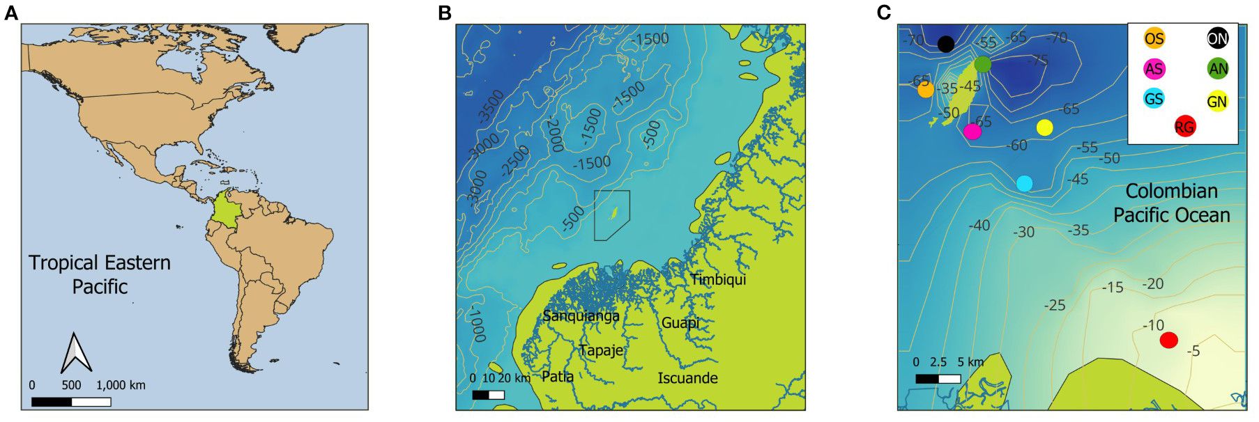
Figure 1. The study area is the Colombian Pacific Ocean (Tropical Eastern Pacific). (A) Location of the Colombian Pacific, as part of the Panama Bight. (B) The polygon representing the protected area of the Gorgona National Natural Park is shown, along with its proximity to the coastline and the main continental watersheds that discharge their waters into the area (marked in blue): Patía River, Sanquianga River, Tapaje River, Iscuandé River, Guapi River, and Timbiquí River. (C) The colored points show the seven stations where discrete water samples were collected from November 2021 to July 2022 along the coast-ocean gradient; Guapi River in red (RG), South Guapi in blue (GS), North Guapi in yellow (GN), South Reef in pink (AS), North Reef in green (AN), South Ocean in orange (OS), and North Ocean in black (ON). The underwater topography lines are represented in meters.

Precipitation on Gorgona Island follows a bi-seasonal pattern (periods of less and more rain), with an annual total rainfall up to ~6000 mm (Blanco, 2012). At seasonal scale, we performed a multi-year analysis of precipitation on the Gorgona Island (2006-2021, data source IDEAM) which indicated low relative rainfall from January to April (Figure 2), when the northern trade winds dominate and the wind field of the Chocó Jet is weak. In contrast, the period with higher precipitation conditions were found from May to December (not shown), when the southern trade winds dominate and the Chocó Jet winds are stronger (September to October). Figure 2 shows extreme precipitation during the 2021–2022 sampling year, with monthly rainfall exceeding 700 mm for several months. Only four months recorded precipitation below the multiannual average (Figure 2B). The precipitation regime on Gorgona Island is primarily governed by the latitudinal migration of the Intertropical Convergence Zone (ITCZ), which provides the context for understanding the atypical precipitation observed. According to Schneider et al. (2014), this pattern dictates that the relative driest period occurs in January and February, when the ITCZ is at its southernmost position (2°N) near the study area (2° 55’ – 3° 00’). Then, from March to May, it moves to the north, occupying a latitudinal range between 2 and 7°N. Conversely, the wettest period is expected between June and July as the ITCZ moves north (reaching 8 to 10°N). Finally, between September and December, the ITCZ returns to its southernmost position.

Figure 2

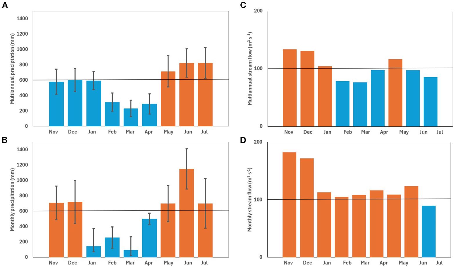
Figure 2. Time scale comparison of precipitation and streamflow (Río Guapi) in the study area. (A) Multiannual total precipitation as monthly averages (2006-2021). The black horizontal line marks the historic (2006-2021) annual mean total precipitation (605 mm) for the “Isla Gorgona station”. Standard deviation is illustrated on each month’s data. (B) Average monthly total precipitation for the sampled year (November 2021 to July 2022). Black horizontal line marks the historic annual mean (2006-2021). Standard deviation is illustrated on each month’s data. (C) Multiannual total streamflow as monthly averages (2006-2021) from the “57025020 Isla Gorgona” IDEAM station. Black horizontal line marks the historic (2006-2021) annual mean discharge (103 m^-³ s^-1). (D) Average total monthly streamflow for the sampling year (November 2021 to July 2022) at the “53047010 Río Guapi” station of IDEAM. Black horizontal line marks the historic (2006-2021) annual mean discharge (103 m^-³ s^-1). Months below the multiannual records are shown in blue, and above in orange.

In the study area, the northeastern trade winds dominate between December and March, generating the Panama Jet, which causes a strong upwelling extending from north to south in the Panama Bight (Rodríguez-Rubio et al., 2003; Corredor-Acosta et al., 2020; Crawford et al., 2023). Similarly, in the second half of the year, the Chocó Jet occurs (Rodríguez-Rubio et al., 2003; Crawford et al., 2023), which travels from west to east until it collides with the continent. The Chocó Jet is strongest in November and weakest between February and March, so the heavy rainfall from November to December on Gorgona Island is attributed to this climatic phenomenon (Crawford et al., 2023). The intense rain creates a layer of brackish water on the surface, up to 2 meters thick (Gassen et al., 2024), which reduces salinity on the Colombian Pacific coast, and river runoff from the Guapi river and deltaic complex into the sea increases. The Guapi River characterized by a sea water temperature of 26.34 °C at 10 meters (Palacios Moreno and Pinto Tovar, 1992), had an average NBS pH of 7.3 between 2018 and 2021, and salinity (PSU) between 0 and 0.25 at 1-meter depth (INVEMAR, 2019, 2020, 2022).

The island is influenced to the east by several rivers and deltas from the mainland, and on the oceanic side (west) by oceanic currents from the Northern Hemisphere, such as the California and Northern Equatorial currents, and from the Southern Hemisphere, by the Peru and Humboldt currents (Diaz, 2001; Willett et al., 2006; Fiedler and Lavín, 2017). The hydrodynamic pattern around the island is dominated by ocean currents and numerous mesoscale eddies, both cyclonic and anticyclonic occurring throughout the year. The direction and intensity of those geostrophic field and mesoscale eddies around Gorgona are determined by wind stress, the Panama Jet, the Chocó Jet, and the position of the Intertropical Convergence Zone (Rodríguez-Rubio et al., 2003; Díaz Guevara et al., 2008; Corredor-Acosta et al., 2011; Lorenzoni et al., 2011). Specifically, the Panama cyclonic current (Amaya, 2024) is fed from the south by a branch of the Peru current, forming the so-called Colombia current (Stevenson, 1970; Corredor-Acosta et al., 2011), which flows from south to north along the Colombian coast. The surface water masses flows through the area of Gorgona National Natural Park in a northeastward direction, with a velocity ranging between 0.2 and 0.9 m s^-1 (Diaz, 2001). During La Niña, the North Equatorial Countercurrent (warm water with high salinity) flowing from west to east (Torres et al., 2023) loses it prevalence around 3°N, while the Peru Current, flowing in a northeastward direction, brings cold water from the South Pacific to the Colombian coast. Therefore, the sampling carried out in this present study (2021-2022) corresponds to a period of relatively cold water (La Niña; ONI -1.0; McLean et al., 2024) contrasting with what happens during El Niño events. Also, at more local scale, the oceanographic circulation is affected by semidiurnal tides (two highs and two lows) oscillating between -40 cm and 5 m per day (Tide-Forecast.com, map of tide stations in Colombia 2021-2022).

According to Restrepo and Kjerfve (2004) and Blanco (2012), La Niña events significantly influences river discharge in the Colombian Pacific due to increased precipitation and, consequently, water flow especially during the sampled year (Figure 2). The Colombian Pacific watershed covers an area of 76,852 km² and consists of more than 200 rivers, which a total discharge of ~9,000 m³ s^-1 and 96 million tons of sediment per year (Díaz, 2008). The Gorgona National Natural Park is in front of the Patía-Sanquianga delta complex, the largest in the country, which contributes approximately 23% of the total freshwater discharged into the Colombian Pacific (2,045 m³ s^-1; Díaz, 2008). The delta complex is made up of the Patía-Sanquianga rivers, which discharge 1,300 m³ s^-1, the Guapi River at 357 m³ s^-1, the Iscuandé River at 213 m³ s^-1, and the Tapaje River at 175 m³ s^-1 (Restrepo and Kjerfvel, 2004; Díaz, 2008; Figure 1). The Patía-Sanquianga delta, covering an area of 23,000 km², contributes freshwater, nutrients, and organic and inorganic material (both particulate and dissolved) from the western Andes mountains to the Pacific Ocean (Restrepo and Kjerfve, 2004; Giraldo et al., 2011). The Guapi River multi-year average monthly flow (station “53047010 IDEAM”) was 103 m³ s^-1 from 2000 to 2021. However, during La Niña event (2021-2022), the stream flow exceeded the multi-year monthly average, with a maximum value in November 2021, exceeding the average by over 77% (182 m³ s^-1), with a minimum in February 2022 being also 2% above the multi-year monthly mean (105 m³ s^-1; Figure 2). On average, the flow exceeded expectations, except for July 2022 when it was 14% below the multi-year average (89 m³ s^-1).

In this context, this study aims to: (1) evaluate the net CO₂ flux in the Panama Bight to address a gap in the current knowledge of the region, as no similar studies have been addressed it in the coastal zone of the Colombian Pacific; and (2) review the predictions made by the models proposed by Wong et al. (2022) and Dai et al. (2022), assessing their accuracy and applicability in the context of this study. To do so, we estimate the seasonal direction and intensity of the CO₂ flux under the effects of La Niña conditions (2021-2022), characterized by intense precipitation and river discharge promoting an estuarine system. Lastly, we discuss the potential drivers explaining the dynamics of the pCO_2w and CO₂ flux variability.

2 Methods

2.1 Sampling design

Seven stations were sampled and used to estimate CO₂ fluxes and carbonate system chemistry in Gorgona National Natural Park from the coast to the open ocean. The closest station to the coast was “Río Guapi - RG”, located approximately 25 km from Guapi-Nariño, Colombia, and the furthest was “North Ocean - ON”, approximately 60 km from the coastline. The stations were distributed along two parallel transects separated by five kilometers, with GPS-WGS84 coordinates. The southern transect was formed by “South Guapi - GS”, “South Reef - AS”, and “South Ocean - OS”, while the northern transect was formed by “North Guapi - GN”, “North Reef - AN”, and “North Ocean - ON” (Figure 1). Monitoring began in November 2021 and extended until July 2022 (nine months), with monthly sampling during the first week of each month. In addition, the “Río Guapi” station was added in January 2022 to characterize its influence.

2.2 Measurements

On site, salinity, temperature, pH millivolts (total protons), percent oxygen, and depth were measured using a Hanna multiparameter sounder (previously calibrated), a CTD-Castaway, and a YSI equipment (accurate to ±2% of reading or ±0.01 PSU, whichever is greater; ± 0.15 °C; ± 0.02 pH/± 0.5 mV; and ranging from 0.00 to 30.00 ppm (mg/L) with an accuracy of ±0.25% of full range.

Discrete water samples were collected at seven stations (GS, GN, AS, AN, OS, ON, and RG; Figure 1) using a 5 L Niskin bottle at depths between 1.8 and 3 meters. The water collected on site was not murky, sampling sites were right after the river plume limit (35 km away from the continent). Seawater samples were stored in 250 mL borosilicate bottles and preserved with 50 µL of a saturated mercuric chloride (HgCl₂) solution for later TA analysis in the laboratory, following recommended best practices (Best Practice Guide for Ocean CO₂ Measurements, SOP 2, SOP-specified concentration range of 0.02-0.05%). Additionally, DIC samples were taken in 50 mL dark bottles (silicone seal), leaving no headspace; and wrapping the cap in parafilm paper. All samples were packed in a Styrofoam refrigerator and sent by plane to our new lab in Bogotá (Javeriana University) in less than four hours from the Pacific region. Then, the samples were kept without exposing them to light and maintaining temperature conditions below 15 °C in the laboratory. TA was measured within two weeks, as well as other parameters such as pH. Regarding DIC samples, those were kept in our lab for two months after the sampling was finished and then sent to the Autonomous University of Baja California in Mexico. They were processed in a maximum of one week after arrival in the UABC.

In the laboratory, total alkalinity (TA) measurements were performed on seawater samples following a standardized protocol (SOP 3b of the open-cell titration method; Dickson et al., 2007) using the GOA-ON titration kit. For titrant, Dickson Lab reference HCl solutions were used (Batch A17: 0.100362 ± 0.000009 mol kg^-1; Batch A24: 0.099922 ± 0.000005 mol kg^-1), buffered with 0.6 M NaCl to match seawater ionic strength. A 50 g sample (~50 g or mL, ± 0.0001 mL) was weighed into a jacketed titration cell (maintained at ~25 °C via a circulating water bath) and titrated. The analytical balance used (Ohaus Pioneer AX225D, ± 0.0001 g) yielded a reproducibility of ±0.001 g for 50 g samples, corresponding to a coefficient of variation<0.003%, well within the precision requirements for TA analysis (0.01 g). The titration involved two stages: first, the addition of a small amount of acid (0.2 mL) with a HandyStep^® Touch S, first by adding to drop the pH to ~3.5 (~0.2100 mV) and waiting 5 minutes to allow for degassing, and second, titration resumed in 0.05 mL steps until a pH close to 3.0 was reached (~0.2300 mV), with pH and temperature measurements taken at each step. Data, including sample volume, titrant volumes (to pH 3.5 and 3.0), salinity, final temperature, and voltage per addition was compiled in an Excel spreadsheet program, which employed a non-linear least squares regression to calculate total alkalinity (Dickson et al., 2007). Approximately 50% of surface samples (n = 31) were analyzed in triplicate. Only triplicate sets with a maximal variation of ±5 µmol kg^-1 TA were retained (± 9 μmol kg^-1, Batch #182: 2230.91 ± 0.71 µmol kg^-1; Batch # 202: 2215.13 ± 0.57 µmol kg^-1; all data set available at NOAA; https://doi.org/10.25921/gfan-3e30).

Dissolved Inorganic Carbon (DIC) was measured at UABC (Mexico) using the UIC C-CM5014 instrument, following the coulometric methodology described by Johnson et al. (1987) and Dickson et al. (2007). Measurements were performed with high precision and accuracy, ensuring that the difference in DIC from the reference values ​​of the standards did not exceed 3 μmol kg^-1 (error of 0.1%). The Dickson Certified Reference Material (CRM) was prepared at the Institute of Oceanography, University of California, San Diego (USA). The substandards and analyzed samples were carried out in parallel at the Oceanographic Research Institute of the Autonomous University of Baja California (Mexico). For a more comprehensive DIC measurement methodology, see Supplementary Table 1.

Similarly, quality “flags” (scale 1 to 5) were reviewed and assigned to the TA and DIC data (equipment accuracy and potential errors in the field or laboratory). Outliers (n=6) were removed from the matrix; this was done by reviewing multiple graphical relationships between temperature, salinity, TA, and DIC.

The Liss and Merlivat (1986) equation allowed for the calculation of the flux magnitude for each of the nine months and seasons in Gorgona. The estimated CO₂ flux in Gorgona was compared with the IPACOA, OOI, NOAA, and SOCAT databases.

The CO₂ fluxes (FCO₂ direction, magnitude, and variability) were calculated following the equation proposed by Liss and Merlivat (1986):

$$FC{O}_2=k\times K^{\prime }\times (\Delta pC{O}_2)(mmol·m^2·yea{r}^{-1})$$

Where, the constant k is the gas transfer coefficient of CO₂ as a function of wind (U₁₀) at 10 meters above sea level (Wanninkhof, 2014), expressed as:

$$k=0.251(\frac{Sc}{660})0.5{(U_{10})}^2$$

K′ is the solubility of CO₂ and is a function of temperature and salinity (Weiss, 1974); Sc is the Schmidt number and depends on temperature; ΔpCO₂ is the difference between the partial pressure of carbon dioxide (pCO₂) in the surface seawater (pCO_2w) and the pCO₂ of the atmosphere (pCO_2A). ΔpCO₂ determines the direction of the flux, with positive FCO₂ indicating CO₂ moving from the sea to the atmosphere, and negative indicating movement from the atmosphere to the sea. The magnitude of the gas exchange is controlled not only by ΔpCO₂ but also by the gas transfer rate between the two media, which in turn varies with wind speed.

The hourly wind speed from the seven sampling sites - U₁₀ (m s^-1) was extracted from: https://earth.nullschool.net/, taking the 24-hour wind average of the sampling day. For months with sampling of all stations on two consecutive days (adverse weather conditions in two months), 48-hour wind values were averaged. The wind average was also calculated and compared using only the exact sampling hours at each station and by averaging the wind over a month, finding no significant changes in the flow results compared to the daily/monthly wind average (which was finally used).

Since the atmosphere is a well-mixed fluid, the pCO_2A values for the flow calculation were extracted from NOAA/GML https://gml.noaa.gov/ccgg/trends/data.html (NOAA, 2021, 2022), which come from the Mauna Loa climate station, Hawaii, file “Mauna Loa CO₂ monthly mean data.” The pCO_2A data for the sampling months (Nov 2021 to Jul 2022) were extracted.

The pCO_2w was calculated from TA, DIC, salinity, and temperature data resolving the carbonate system equation in seawater using the CO2SYS v3.0 software (Pierrot et al., 2021). In the carbonate system equation solution, the following constants were used: (i) Dissociation constants for K1 and K2 from Millero (2010) for waters ranging from 0 to 40, given that the study area the salinities variation are between 27.03 to 31.29, (ii) KHSO4 dissociation constant from Dickson (1990), (iii) KHF from Perez and Fraga (2003), (iv) Total pH scale (mol-kg SW), (v) [B]T value from Lee et al. (2010), and (vi) EOS-80 standard. The pCO_2w was estimated with an error of ±1.79 concerning the determined fluxes (mmol C m² day^-1). Out of 66 flux data points, six were flagged as possible outliers (flags three onward). The CO2SYS was also used with DIC and TA pairs to estimate the Revelle factor, omega aragonite (Ω_AR), HCO₃, and CO₃. Lastly, the pH in total scale was derived through the CO2SYS using the same specific settings and found to be less variable than in situ measurements, displaying a smaller error. We performed a full uncertainty propagation analysis, which yielded the following average errors: pH_T (± 0.022), pCO_2W (± 30.17 µatm), total alkalinity (TA: ± 9 µmol kg^-1), dissolved inorganic carbon (DIC: ± 3 µmol kg^-1), salinity (± 0.20 PSU), and temperature (± 0.08 °C). These values fall within acceptable ranges for carbonate system studies and support the reliability of our calculated FCO₂ values at Gorgona.

Daily images of Chl-a were downloaded from the Ocean Colour Climate Change Initiative (OC-CCI; version 3.1) for the studied period. The OC–CCI is a merged Level 3 product with a spatial resolution of 4 km, available at http://www.oceancolour.org/. The OC-CCI Chl-a dataset is retrieved by combining the observational data from the MERIS (MEdium spectral Resolution Imaging Spectrometer) sensor of the European Space Agency, the SeaWiFS (Sea-viewing Wide-Field-of-view Sensor) and MODIS-Aqua (Moderate-resolution Imaging Spectroradiometer-Aqua) sensors from the National Aeronautics and Space Administration (NASA-USA), and the VIIRS (Visible and Infrared Imaging Radiometer Suite) from the National Oceanic and Atmospheric Administration (NOAA-USA). The remote sensing reflectance data derived from the sensors were merged by band-shifting and bias-correcting the MERIS, MODIS, and VIIRS data to match the SeaWiFS data. Due to the complexity of the study region, version 3.1 of the OC-CCI product was selected as it improves the performance of the ocean color data in coastal Case-2 waters compared to earlier versions that primarily focus on open ocean waters. Finally, total monthly Chl-a values were obtaining by averaging the Chl-a of the seven sampling stations, resulting in a relative total Chl-a concentration for the entire sampling region.

2.3 Statistical analyses

The analysis began with a Shapiro-Wilk test, which indicated that the flux magnitude data does not follow a normal distribution (S-W, P = 0.01877, W = 0.95, n = 60), repeating this for pCO_2w and ΔpCO₂ components, respectively (S-W, p = 0.147 and 0.134, W = 0.97 and 0.96, n = 60 and 60), indicating that the variables associated with flux do not follow a normal distribution either. Hence, the Box-Cox methodology was applied to transform FCO₂ data into a normal distribution. Furthermore, a Welch F test in the case of unequal variances was applied to all the variables of interest (FCO₂, pCO_2w, ΔpCO₂, SST, SSS, TA, DIC, and Chl-a) which showed that these different data groups have equal variance (W-F, F = 2.512E^-4, df = 200.3, p = 1.855E^-304). Moreover, a t-test (parametric) was used to analyze differences between the two flux periods: Upwelling (January to March of 2022) and Post-upwelling (November to December of 2021 and April to July of 2022). We used a One-way ANOVA to compare different flux magnitudes across the nine months, and then an a posteriori t-test. Additionally, a Spearman linear correlation was run to explore relationships between pCO_2w and SST, SSS, TA, DIC, and Chl-a.

Normalizations to observe the pCO_2w sensitivity were conducted as follows: we used the maximum values for salinity and temperature (32.06 units and 28.1 °C, respectively) setting the maximum value for salinity first, as a constant, while leaving the TA, DIC, and temperature values corresponding to each data point to evaluate the effect of salinity over the pCO_2w, repeating the same process but substituting the temperature for the recorded maximum, and leaving salinity as measured (CO2SYS). Then, we recalculated the pCO_2w and plot the difference between the pCO_2w with in situ salinity against the recalculated pCO_2w that uses the maximum recorded salinity. 49 µatm higher, in average, was the pCO_2w difference by using max salinity effect. Regarding a normalization with maximum temperature, the same procedure was followed where the maximum recorded temperature was constant, and the remaining variables used the corresponding values, revealing an average pCO_2w difference of 31 µatm higher than with the observed temperatures (Supplementary Figure 1) in the CO2SYS (Lewis and Wallace, 1998). Thus, it is clear that salinity has a larger influence (relative percentage) than temperature regarding the pCO_2w variability observed throughout the year. To complement these normalizations, we assessed the uncertainty associated with pCO_2w by incorporating the potential error of ±30.17 μatm into our flux calculations, recalculating them and comparing them to the original estimates.

In addition, to define climatic-oceanographic periods, a Principal Component Analysis (PCA) was performed using the latest version of R Studio software. The PCA used the following variables: month, season, SST, SSS, pCO₂w, pH_T, DIC, Chl-a, to review if there are spatio-temporal FCO₂ groups. Furthermore, to clearly separate both seasons we used several atmospheric/climatic variables, such as total monthly precipitation (mm), average sea surface temperature (SST), average pH (total), average surface water partial CO₂ pressure (pCO_2w), and average CO₂ fluxes (mmol m^-2 d^-1).

2.4 Zonal Ekman Transport and Ekman pumping

The Zonal Ekman Transport (ZET) was obtained following the methodology of Bakun and Nelson (1991) by using weekly wind data obtained from the CCMP product (https://www.remss.com/measurements/ccmp/). For the calculation, we follow the equation:

$$ZET=\frac{1}{{\rho }_{w}f}\tau$$

where ρ_ω is the density of seawater, which is assumed constant at 1025 kg m⁻³; f is the Coriolis parameter and τ is the wind stress for the studied area.

The wind stress (τ) was computed from the weekly wind fields as follows:

$$\tau ={\rho }_a{C}_d\left|V_{10}\right|V_{10}$$

where C_d = 0.0015 is the drag coefficient, ρ_a = 1.2 kg m⁻³ is the mean air density, and V₁₀ is the wind speed at 10 m above the sea surface. The wind stress curl was estimated using the zonal and meridional components of the weekly wind stress:

$${(\nabla \times \tau )}_z=\frac{\partial {\tau }_y}{\partial x}-\frac{\partial {\tau }_x}{\partial y}$$

This procedure was performed for each grid point of the wind field by applying the centered finite difference algorithm, and the Ekman pumping velocity was estimated as follows:

$$WEK=\frac{{(\nabla \times \tau )}_z}{f{\rho }_w}+\frac{\beta {\tau }_x}{f^2{\rho }_w}$$

where τ_x is the zonal wind stress component, β = (2Ωcosφ/R) is the latitudinal variability of the Coriolis parameter (f = 2Ωsenφ), R = 6,371,000 m is the radius of the earth and ρ_w = 1025 kg m⁻³ is the mean water density. This methodology has been previously used on the Northeast Tropical Pacific (Kessler, 2006) and Panama Bight region (Devis-Morales et al., 2008; Corredor-Acosta et al., 2020).

Previous studies have indicated an interplay between the Ekman transport due to alongshore winds and Ekman pumping due to offshore wind stress curl playing an important role due to their relative contributions for upwelling/downwelling dynamics. For instance, in the northern Chilean upwelling system, the vertical transport induced by coastal divergence (ZET) represented the 60% of the annual total upwelling, however, the Ekman pumping also displayed an important contribution of 40%, indicating that the largest differences between these mechanisms occur at spatial scale. That is, coastal ZET predominated in areas with low orography and headlands, whereas WEK was higher in regions with high orography and the presence of embayments (Bravo et al., 2016). Similar findings were observed in three typical upwelling systems of the South China Sea, showing temporal and spatial differences, highlighting regions where WEK had the same intensity as ZET, even doubling the amount of upwelling predicted solely considering the coastal divergence (Wang et al., 2013). Those physical mechanisms and their coupling are important to be explored because the physical transfer of water properties and nutrients from the deep to the surface ocean is strongly related to the vertical supply, which also involves important effects on primary productivity, changes in the water column mixing/stratification and associated water masses, as well as, in the local chemical processes (e.g., Williams and Follows, 2003; Pasquero et al., 2005). According to this, we assess both mechanisms (ZET and WEK) in this study, in order to relate its contributions to the maintenance of biological production (in terms of Chl-a) and key changes of the carbonate system.

2.5 Mix model

To identify potential processes (physical mixing and biological) and explain the variability observed in carbonate system parameters (e.g., pCO_2w, DIC, TA, and O₂), we employed a three-endmember mixing model following established methodologies in oceanographic studies that developed the analysis of sea water from mixing triangles without assumption of isopycnic mixing (Tomczak, 1981; Paulmier et al., 2011; Kahl et al., 2018). This approach identifies water endmembers, in order to describe the thermohaline variability due to mixing, using conservative tracers (salinity and potential temperature) to construct a mixing triangle. The contribution of the water masses considered (M_k,i) to a given sample ‘i’ can be calculated by solving the followings determined system of three linear equations:

$$1= \text{Σ} M_{K,i}$$

$$S_i=\text{Σ} M_{K,i}· S_k$$

$${\theta }_i=\text{ Σ} M_{K,i}· {\theta }_k$$

Where k is the water mass endmembers (1,2 and 3) and ‘i’ is the sample number (from 1 to 60). S_k and θ_k are the thermohaline characteristics of the k-water mass endmember (Tomczak, 1981). Finally, it computes expected conservative values due to physical mixing processes (DIC_mix, TA_mix, and O_2mix) for the non-conservative variables measured in situ (DIC, TA, and O₂). DIC_mix is defined as the fraction of dissolved inorganic carbon whose variability (R² from the regression DIC_mix vs. DIC) can predominantly be attributed to physical mixing. The complementary variability (1 – R²) is then attributed to biogeochemical processes, isolated through residual analysis (e.g., ΔDIC = observed DIC – DIC by mixing) and quadrant plots of ΔDIC vs. ΔO₂, where quadrants indicate net production (positive ΔDIC, positive ΔO₂), photosynthesis (negative ΔDIC, positive ΔO₂) ammonification (negative ΔDIC, negative ΔO₂) or respiration/remineralization (positive ΔDIC, negative ΔO₂) (Paulmier et al., 2011; Kahl et al., 2018).

Initially, we constructed T-S diagrams from the full spatiotemporal dataset (13 months, 7 stations, 0–80 m depth) to define three endmembers representing distinct sources of variability and mixing in the area. The river endmember (1; river-influenced) exhibited low salinity (26.81), TA (1750 µmol kg^-1), and DIC (1763 µmol kg^-1), with high temperature (27.94 °C) and O₂ (174 µmol kg^-1). The transitional endmember (2) showed intermediate values: salinity (33.06), TA (2138 µmol kg^-1), DIC (1867 µmol kg^-1), temperature (27.28 °C), and O₂ (123 µmol kg^-1). Finally, the oceanic endmember (3; oceanic influenced) featured high salinity (35.38), TA (1999 µmol kg^-1), and DIC (1989 µmol kg^-1), with low temperature (14.26 °C) and O₂ (40 µmol kg^-1; Preciado et al., in Progress). All three water endmembers incorporate signals from multiple upstream sources, reflecting the complex dynamics of this estuarine system. For instance, the oceanic (3) endmember exhibited influence from at least four diverse origins, including Antarctic Intermediate Water signals (Kawabe and Fujio, 2010); the intermediate endmember (2) blends subsurface and riverine inputs; and the river endmember (1) primarily mixes freshwater with marine waters, potentially including remote eddy-transported surface waters and local coastal currents. We could not directly measure riverine carbonate parameters due to differences in instrumentation and chemistry, river itself even showed tidal intrusion of seawater from below during high tides, further complicating pure freshwater end-member isolation. Instead, riverine influence is inferred through its dilution effects on salinity and biogeochemistry, following a similar approach to Huang et al. (2022) and Sun et al. (2023).

Once the mixing fractions are applied to compute expected DIC_mix values under conservative mixing assumptions. Deviations from these expected values then highlighted non-conservative processes affecting DIC, which is a key objective of our biogeochemical analysis. DIC, TA, and O₂ are used as complementary information for the characterization of the endmembers, enabling us to perform the mixing model analysis and determine the sources of variability (physical-mixing or biogeochemical processes) for the non-conservative variables DIC, TA, and O₂. This approach aligns with standard practices in estuarine and oceanic studies, where salinity and TA are often normalized or used to account for dilution and mixing effects before assessing non-conservative variables like DIC (Cai & Wang, 1998; Oliveira et al., 2017; Courtney et al., 2021). For instance, while TA behaves conservatively in many open-ocean settings and correlates linearly with salinity (Millero et al., 1998; Jiang et al., 2014), the T-S framework was chosen due to its effectiveness in capturing thermohaline distinctions in Pacific Colombian dynamic estuarine system, influenced by high rainfall and runoff. In addition, to validate the implication of the biological removal in pCO_2w concentration, we used a complementary approach, such as ΔDIC together with cumulative monthly in situ Chl-a data to explain CO₂ consumption. These results (biological/temperature implications) were also validated by an analysis to calculate if physical or biological factors are implicated in the pCO_2w concentrations found around Gorgona island, following the methodology described by Takahashi et al. (2002), for more detail on the equations used see Supplementary Table 2.

3 Results

The PCA (Figure 3) revealed two distinct seasonal clusters: an upwelling period (January–March) and a post-upwelling period (May–July, November–December) distributed across the space. Together, PC1 (45.5%) and PC2 (28.2%) explained 73.7% of the total variability. The biplane shows that post-upwelling months were characterized by warmer, CO₂-enriched surface waters, whereas upwelling months reflected cooler, saltier, DIC-rich conditions and elevated pH_T. Chlorophyll-a displayed an intermediate position, reflecting its role across both seasons. No spatial separation among sampling sites was detected, implying that despite local variability, temporal changes through upwelling and post-upwelling dynamics (e.g. rainfall and stratification) were the main driver of environmental variability around Gorgona Island.

Figure 3

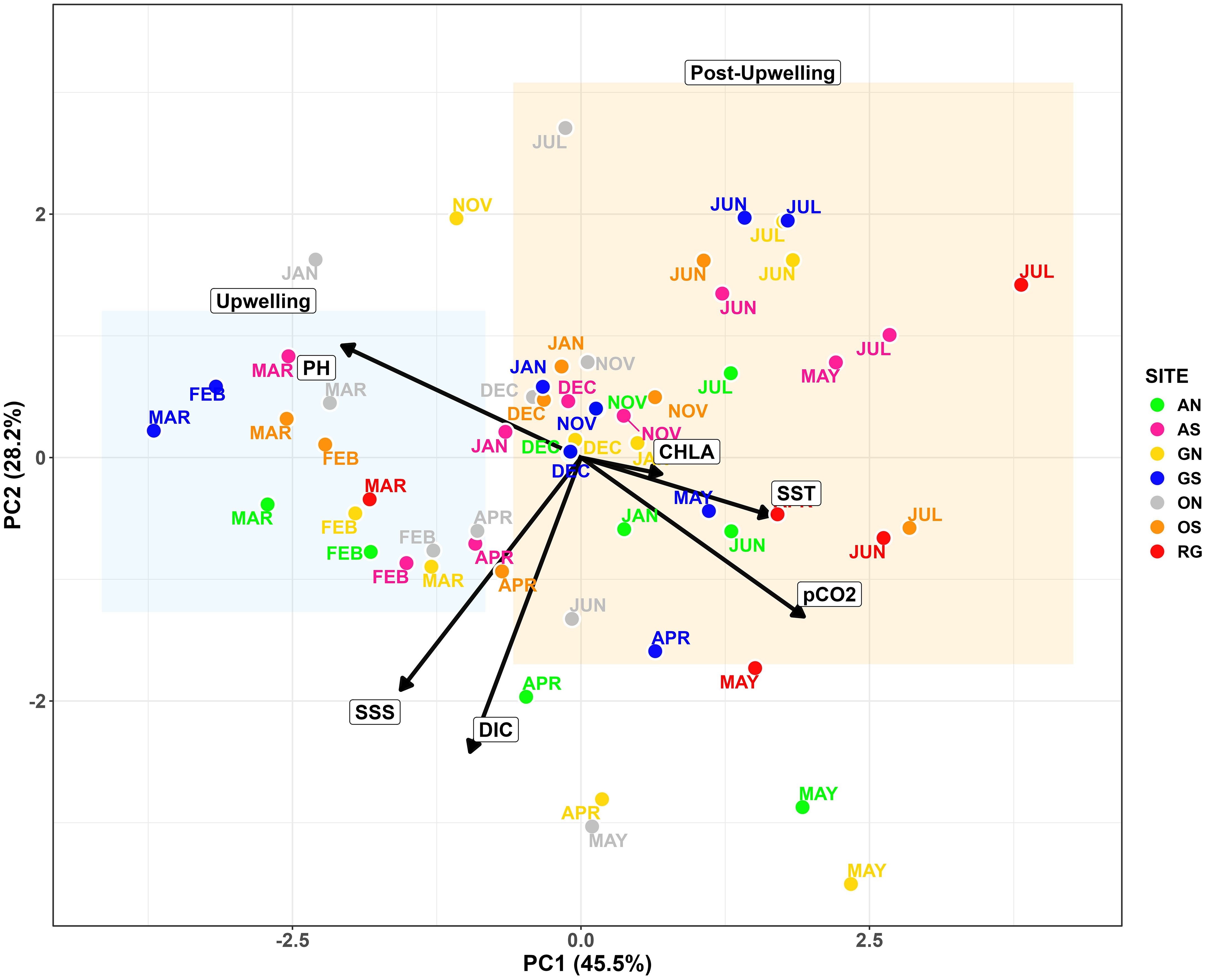
Figure 3. PCA test for stations and months considering the physicochemical variables SST, SSS, pCO₂, pH, DIC, and Chl-a. Note the grouping in the left quadrants for the months of February and March (upwelling, blue rectangle), from the upper right quadrant, May, June, and July (rainier season; post-upwelling, orange rectangle), highlighting the two contrasting seasons. The x axes explain the main variability 45.5% and the second axis y 28.1%. The colors represent the different sites and their corresponding sampling months.

The two seasonal periods were verified through the atmospheric/climatic variables showing significant differences between upwelling and post-upwelling. That is, total monthly precipitation (M-W, Z = 2.203, p = 0.027, n Post-upwelling = 6 months, n Upwelling = 3), average sea surface temperature (SST; M-W, Z = 2.2132, p = 0.0268, n Post-upwelling = 6, n Upwelling = 3), average pH (total; M-W, Z = 2.2039, p = 0.027532, n Post-upwelling = 6, n Upwelling = 3), average surface water partial CO₂ pressure (pCO_2w; M-W, Z = 2.1947, p = 0.028186, n Post-upwelling = 6, n Upwelling = 3) and average CO₂ fluxes (mmol m^-2 d^-1; M-W, Z = 2.0045, p = 0.071429, n Post-upwelling = 6, n Upwelling = 3). Specifically, during post-upwelling we found significantly higher: (I) Monthly average precipitation (746 ± 214 vs 165 ± 82 mm) due to the increased influence of the ITCZ and a moderate La Niña year; (II) Average sea surface temperature (27.5 ± 0.4 °C vs. 26.5 ± 0.2 °C); and (III) Average pCO_2w and CO₂ Fluxes (567 ± 64 μatm vs. 450 ± 55 μatm, and 0.2 ± 0.09 mmol CO₂ m^-2 d^-1 vs. 0.1 ± 0.06 mmol CO₂ m^-2 d^-1, respectively). Contrasting, in upwelling, we found a higher significant total pH mean (7.8697 vs 7.9686, respectively).

3.1 Air–sea CO₂ exchange

During the moderate 2021–2022 La Niña event, surface waters around Gorgona displayed a near-neutral net CO₂ flux (0.0105 ± 0.0001 mol C m^-2) over the nine sampled months, with a bimodal pattern driven by upwelling and post-upwelling wet season (Figure 4). Throughout the upwelling season, cooler, saltier waters reached the surface (shallow thermocline), coinciding with the observed low pCO_2w values (below atmospheric levels, mean pCO_2A = 461 ± 92.8 μatm and negative ΔpCO₂, see Figures 4A–E), resulting in near-zero to weakly negative FCO₂ (February–March, Figure 4F). This is additionally in line with elevated DIC and TA (Figures 4G, H). In contrast, during the post-upwelling period, the fluxes were slightly positive (0.0093 ± 0.0001 mol C m^-2) with an average pCO_2w of 567 ± 97.5 μatm (Figure 4D). Similarly, monthly fluxes also differed significantly between periods (Welch test, F = 2.5 × 10^-4, p< 1 × 10^-300; n = 9), peaking in June (2.5 mmol C m^-2 month^-1) and reaching a minimum in March (–0.1 mmol C m^-2 month^-1). Therefore, markedly higher fluxes were observed during the post-upwelling compared to the upwelling season when including the seven stations sampled per month (t = 4.91, critical t = 2.00, p = 7.8 × 10^-6; n = 21 vs. 39; Figure 4F).

Figure 4

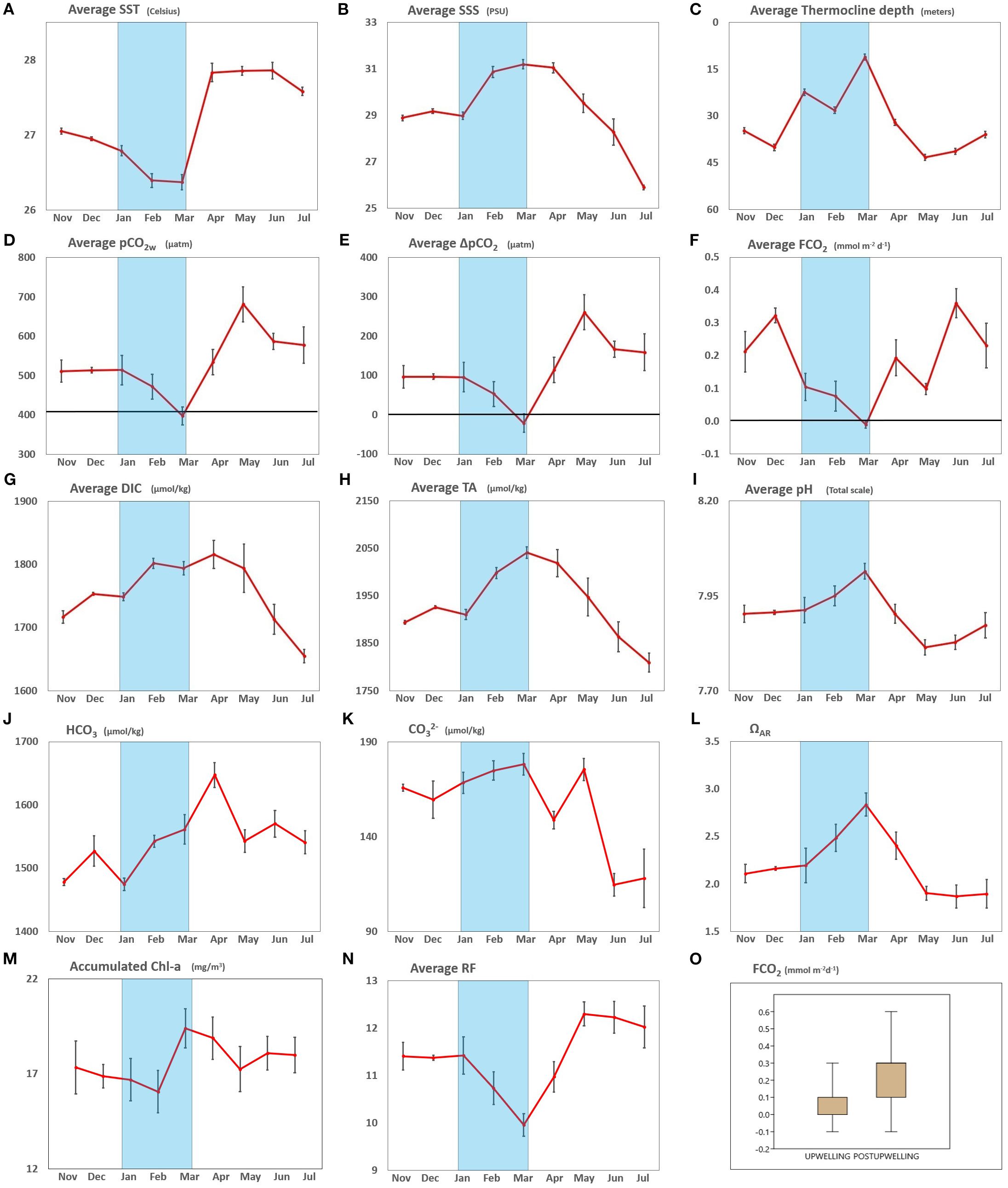
Figure 4. Monthly cycle of: (A) Average sea surface temperature (SST). (B) Average sea surface salinity (SSS). (C) Average thermocline depth (meters). (D) Average pCO_2W with average pCO_2A mark (418 µatm) indicated with a black horizontal line. (E) Average ΔpCO₂ with zero delta mark indicated with a black horizontal line. (F) Average FCO₂ with zero magnitude mark indicated with a black horizontal line. (G) Average Dissolved Inorganic Carbon (DIC). (H) Average Total Alkalinity (TA). (I) Average pH in total scale. (J) Average bicarbonate (HCO3). (K) Average carbonate (CO32-). (L) Average Saturation state of aragonite (ΩAR). (M) Accumulated Chlorophyll concentration (Chl-a). (N) Average Revelle Factor. (O) Boxplot comparing FCO2 values between upwelling (January, February, March) and post-upwelling (November, December, April, May, June, July) evidencing statistical differences (T test, T = 4,908, Tc = 2.001, p = 7.80E-6, N = 21 vs 39, respectively). Monthly measurements around Gorgona near the surface (≤ 3 m), standard error is illustrated as a black vertical line on each data point. Note that Ω AR data starts above 1.2, indicating possible but suboptimal calcification throughout the sampled period.

Comparably, the average pCO_2w trend (Figure 4D) during the upwelling season evidences surface pCO_2w hovering moderately above atmospheric values in January (near 513 µatm Figure 4D; atmospheric reference value ~418 µatm, horizontal black line), but dips towards/just below atmospheric level by March (minimum average 397 µatm). Correspondingly, a post-upwelling spike in pCO_2w increases values up to ~700 µatm in May, around 1.7 times higher than atmospheric values, which drives a large positive ΔpCO₂ and outgassing (Figure 4E). Thereafter, pCO_2w slightly decreases until July, but remains well above atmospheric values (~580 – 590 µatm).

The ΔpCO₂ values in eight of the nine months were above the atmospheric pCO_2A - (between 50 and 260 micro atmospheres). However, during the upwelling season, there is a reduction in pCO_2w, causing it to be less saturated than the pCO₂ of the surrounding atmosphere. Thus, March evidenced less pCO₂ in the water than in the air (negative ΔpCO₂, Figure 4E) which is reflected with near-zero/negative FCO₂ (Figure 4F). Transition to the post-upwelling (higher rain and streamflow season; April-July) was also evident through the progressive increment in CO₂ peaking during May (ΔpCO₂ ≳ +250 µatm; more pCO₂ in the ocean than in the surrounding air) and then stabilizing, as reflected in the average CO₂ flux (Figure 4F).

3.2 Physical oceanographic conditions of sea surface temperature and salinity

The coolest temperatures were recorded during upwelling (~26–26.5 °C). Rapid warming of the surface water was observed in April (~28 °C) lasting until July (>27 °C). The shown warming is concurrent with the sharp rise in pCO_2w (Figures 4A, D). Average salinity was< 31 during the nine months, meanwhile, the highest salinity was recorded during upwelling (31.2 in March). From April to July (post-upwelling months) a steady drop in salinity was measured, coinciding with the peak of precipitation/river discharge (Figure 2). Hence, markedly brackish water was observed (low-alkalinity via dilution), related to pCO_2w increase (Figures 4B, D, H).

3.3 Key parameters of the carbonate system: total alkalinity, pH_T, and dissolved inorganic carbon

The highest pH_T was measured in March (8.01), chemically consistent with reduced pCO_2w values and less riverine/precipitation influence (Figure 4I). Then, pH_T began to decline during April and May (recorded a minimum of 7.81 in May) and stabilized after during June and July. Meanwhile, DIC start increasing between November and January (~1,700–1750 µmol kg^-1) reaching its highest values in April (1,815 µmol kg^-1) and May (~1800 µmol kg^-1). After, there was a general decrease from May onward (~1,790–1,650 µmol kg^-1 by July; Figure 4G).

The dominant DIC species, bicarbonate (HCO₃^-), remained relatively stable from November to February (~1,550–1,600 µmol/kg, Figure 4J) then increased sharply from March–April (~1,720 µmol/kg) in line with the highest DIC/TA values. Thereafter, HCO₃^- decreased gradually during the post-upwelling season (May–July) mirroring the reduction in DIC/TA.

Carbonate ion (CO₃^2-) values showed a clearer seasonal signal. They peaked during the upwelling months (January–March: ~170 and 180 µmol/kg, Figure 4K) in agreement with higher pH_T and Ω_AR (Figures 4I, L). Afterwards, CO₃^2- concentrations decreased during the post-upwelling period, sharply decreasing in April to ~150 µmol/kg, then rebounding slightly during May to ~170 µmol/kg, and finally steadily decreasing to its minimum values from June to July (114–118 µmol/kg) coinciding with lower pH_T, elevated Revelle Factor, and reduced Ω_AR.

3.4 Biological proxy signals

Monthly accumulated Chl-a (sum of seven stations) was relatively high during the sampling period (~16–19 mg m^-³, Figure 4M), with average Chl-a of 1.09 – 2.77 mg m^-³ per sampled site (see Supplementary Figure 2). A marked increase from February to March was observed (16 – 19.4 mg m^-³). Afterwards, Chl-a values remain high during May (17.2 mg m^-³) until July with ~18 mg m^-³ (Figure 4).

3.5 Key chemistry parameters of oceanic chemistry: Revelle Factor and omega aragonite

The Revelle Factor (RF, Figure 4N) and Ω-aragonite (Ω_AR) displayed an inverse relationship. The lowest RF values (9.9) occurred in March, coinciding with weakened or even collapsed stratification (Figure 4C), when Ω_AR reached its peak (2.8). In contrast, RF increased during the post-upwelling season, rising from April and reaching ≥12 by July, concurrent with the lowest Ω_AR values (1.9), indicating suboptimal conditions for calcification. As expected, Ω_AR was inversely proportional to pH_T (Figures 4I, L), while RF varied inversely with SST.

3.6 Seasonal drivers of the carbonate system variability

Seasonal variability in dissolved inorganic carbon (DIC), its mixing component (DIC_mix), and related drivers highlighted the coupled influence of physical circulation and biological activity (Figure 5). During the upwelling season, lower ΔDIC values coincided with reduced pCO_2w and CO₂ fluxes, whereas in the post-upwelling season both DIC and pCO_2w increased together with intensified Ekman transport and pumping (Figures 5B–D). Regional chlorophyll-a distributions also followed these seasonal shifts, with peaks during February–March and again in May–July (Figure 5C).

Figure 5

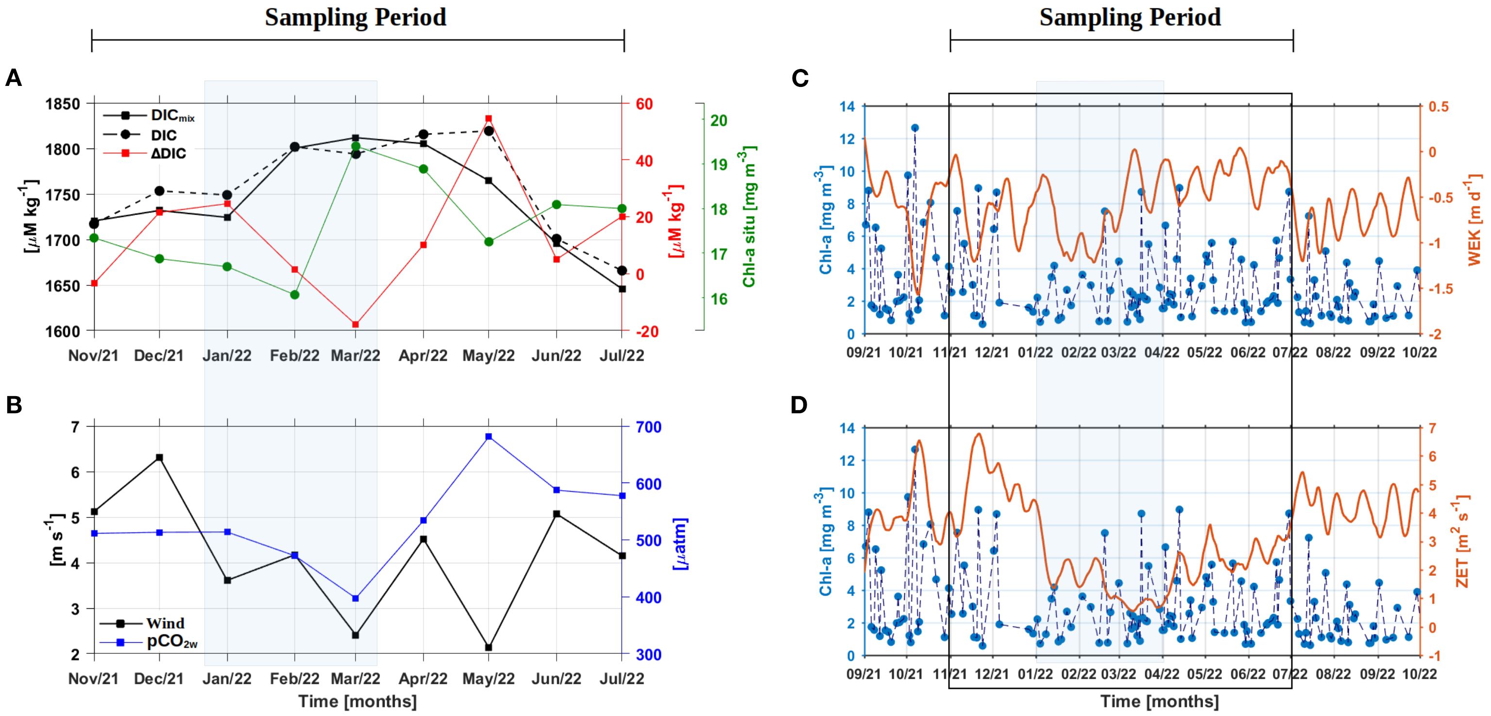
Figure 5. Temporal variability of DIC, DIC_mix, DeltaDIC and accumulated in situ Chl-a values in (A). Monthly average values of wind and pCO_2w of the in situ sampling stations in (B). For comparison and higher resolution analysis, weekly data of regional satellite Chl-a data from the OC-CCI product (https://www.oceancolour.org/) was coupled with weekly Ekman pumping (WEK in C) and Zonal Ekman Transport values (ZET in D). Weekly wind fields for the above calculations were obtained from the CCMP Wind Vector Analysis Product (https://www.remss.com/measurements/ccmp/). Note that the left-panels consider the in situ sampling period between Nov/2021 to Jul/2022, while the right-panels consider a full year of variability including months before, during (black rectangular box), and after the sampling period (Sept/2021 to Sept/2022). Transparent blue rectangle indicates the upwelling period from January to March 2022.

Complementary evidence from a temperature–salinity (T–S) diagram (Figure 6A) underscored the role of mixing in shaping carbonate chemistry. Mixing calculations indicated that up to ~79% of the observed DIC could be explained by conservative mixing of three endmembers, while the residual ~19% reflected non-conservative processes (Figure 6B). The correlation between ΔDIC and ΔO₂ (Figure 6C) suggested that aerobic remineralization and nitrification were the dominant biological drivers of this residual variability. Physical processes dominated DIC variability, as indicated by the strong correlation between DICmix and DIC (R² = 0.79, Figure 6B). In contrast, respiration explained a smaller but measurable fraction of the variance (ΔDIC–ΔO₂, R² = 0.19; Figure 6C). Together, these results highlight that both physical and biological controls on DIC ultimately influenced its relationship with pCO_2w, consistent with the significant negative correlation observed between the two variables (Q = –0.71, p< 0.001, n = 60; Figures 4D, G).

Figure 6

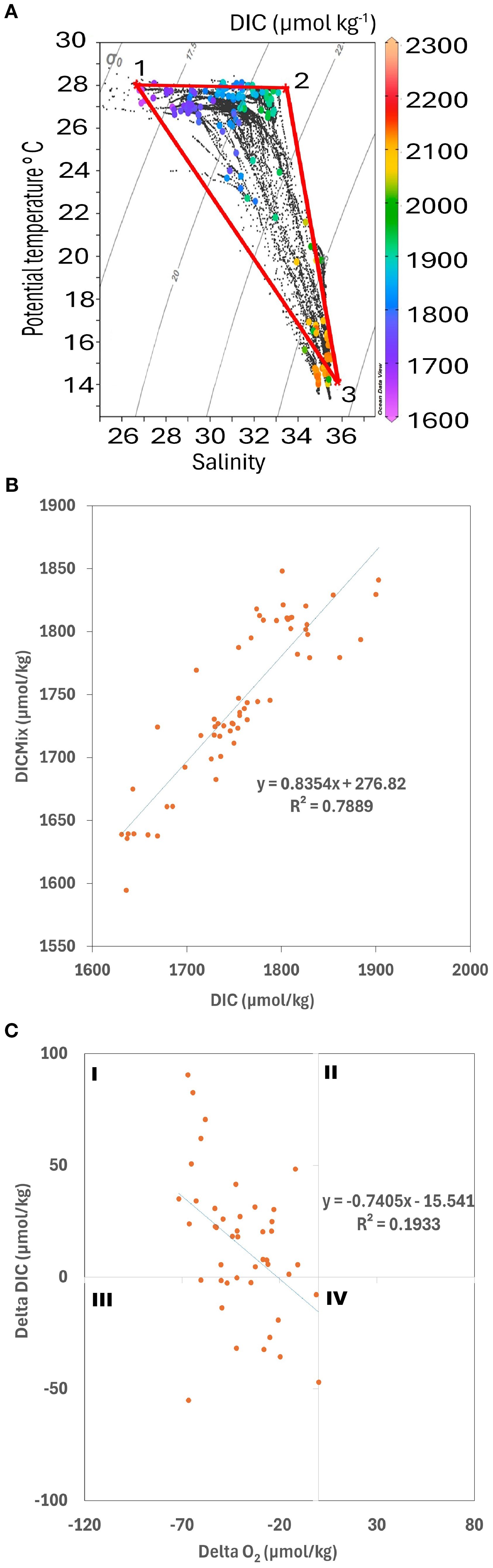
Figure 6. Temperature-salinity (T-S) diagram (A). Data points color-coded by dissolved inorganic carbon (DIC) concentration (μmol kg^-1). The points represent observed oceanographic sampled depths throughout the year. The numbered labels (1-3) denote the end members of distinct water masses, with their respective salinity (S), potential temperature (T), and DIC values. The solid red lines connecting these end members outline the considered mixing triangles. Positive regression between DIC_mix and DIC (B). Physical process explains 78.8% of the DIC measured (DIC_mix). The remaining percentage is explained by biogeochemical processes (19%). ΔDIC (biological processes) and ΔO₂ (µmol/kg) relationship (C; explaining 19%), where sampling points were mainly distributed within quadrants I and III (as shown in Kahl, 2018), suggesting aerobic remineralization and nitrification, respectively.

4 Discussion

4.1 DIC dynamics

The physical mixing of the water mass contributes significantly to explaining the DIC values ​​in the system (Figure 6A) as validated by the relationship between DIC_mix and DIC (Figure 6B; ~78% of variability) and the seasonal variability of WEK and ZET (Figures 5C, D). Therefore, DIC increased from November to May (Figure 5A) and then decreased from June to July. During La Niña 2021-2022, estuarine dynamics were strongly modulated by horizontal and vertical exchanges between marine and freshwater sources. High-frequency tides (up to 4 per day, with amplitudes of 5 m; Cauca tide table 2021–2022) mixed riverine and oceanic waters, while mesoscale eddies and Ekman-Zonal transport introduced deep offshore waters into the system (Corredor-Acosta et al., 2020; Figures 5C, D). Wind speed and direction generate local coastal currents, with north-south surface flow above the thermocline and south-north flow in subsurface waters (in situ observations); and upwelling and subsidence cycles (downwelling; Figures 5C, D) producing three water masses with different densities along the vertical profile (up to 80 m; see Figure 6A). Peaks in DIC between January and March coincided with intensified WEK and ZET which enhanced vertical injection of CO₂ and TA rich subsurface waters, when freshwater dilution and stratification was weaker (lower relative rain and precipitation; Figures 2B, D). Even so, elevation of DIC values could also be due to a gradual increase of bicarbonate and carbonate in the system (Figures 4J, K), when acidic sub-superficial waters (Ω_AR values sometimes below 1.5, Preciado A., unpublished data) could dissolve the reef structure, bringing the increased DIC signal to the surface. From April to July, the relative decrease in DIC reflected dilution by enhanced river discharge and weaker zonal inputs. The residual variability (~19%) was linked to respiration and remineralization, as evidenced by the correlation between ΔDIC and ΔO₂ where DIC increased but O₂ decreased (Figure 6C; O₂ levels reached 60 µmol/kg) and pCO_2w values were elevated. However, this respiration hypothesis requires further studies in the study site, to understand its contribution in DIC variability.

4.2 Seasonal FCO₂ variability

The seasonal variability of FCO₂ in Gorgona during the study period resulted from the system shifting from post-upwelling, dominated by southerly trade winds, higher precipitation and river dominated system to upwelling, dominated by northern winds, less precipitation, and lower river discharge, and then back to post-upwelling season. During post-upwelling, a slight positive increase in FCO₂ is related to the extensive plume of water from coastal rivers (Figure 2) originating from a 44% increase in river flow during the study period (e.g., the Guapi River with 103 m³ s^-1; Figure 2D), this plume extended for more than 60 km from the coast (as observed by floating logs on the field), forming a large estuary with an average salinity of 29.51 units (SD ± 1.56). Thus, following the definitions of Dai et al. (2013) and McKee et al. (2004), our study area can be classified as a system dominated by riverine inputs. During the post-upwelling season, pCO_2W values ​​were relatively high (Figure 4D), ranging from 378 to 839 μatm (average 567 μatm), peaking in May, in line with high SST (Figure 4A), and ΔpCO₂ ranging from 47 μatm to 418 μatm. Our results agree with Ricaurte-Villota et al. (2025), where rivers via remineralization could explain the high pCO_2w values ​during moderate La Niña years (see Figure 6C). But also, the increased freshwater discharge could also diminish CO₂ fluxes, simultaneously, under La Niña (Reimer et al., 2013; Ricaurte-Villota et al., 2025), via nutrient excess and phytoplankton bloom. During upwelling season, the average water temperature decreased to 26.53 °C, but the average salinity remained below 30, confirming the rivers influence on surface waters. Likewise, the pCO_2W was relatively lower, ranging from 316 to 626 μatm (average 461 ± 92 μatm), with minimum values ​​in March, coinciding with the lowest surface temperature (26.11 °C) and highest salinity (28.39). During this period, FCO₂ reached negative or near neutral values (between 0.3 and -0.1 mmol m^-2 d^-1), with similarly low ΔpCO₂ values, ranging from –101 μatm to 93 μatm. Despite theory indicating that upwelling during a moderate La Niña should increase the CO₂ flux to the atmosphere (Kim et al., 2017), this was not observed in our study site. Similar dynamics i.e., low or negative net fluxes despite upwelling have been reported in tropical estuarine systems where upwelled DIC is rapidly consumed by phytoplankton blooms which counterbalance the physical delivery of dissolved carbon (e.g., Vargas et al., 2007; Bouillon, 2011; Giraldo et al., 2011). Monthly patterns and flux directions were preserved when calculated using the propagated pCO_2w error, including the neutral/slight sink observed in March, with only December and June showing greater variability. Net flux differences over the nine-month period remained negligible (original net flux = 0.0105 mol C m^-2, positive error net flux = 0.0133 mol C m^-2, negative error net flux = 0.0077 mol C m^-2) indicating a net total difference of ±0.0028 mol C m^-2, confirming the robustness of our results.

4.3 Temporal pCO_2W variability and key associated variables: salinity, temperature, dissolved inorganic carbon and ΔO₂

The temporal variability of pCO_2W was shaped by the combined effects of salinity, temperature, DIC, and ΔO₂ variables were correlated with pCO_2W values. Salinity showed the strongest and most significant correlation with pCO_2w (Q = –0.96; p = 1.77E^–36, n = 60) reflecting the strong influence of river discharge and freshwater dilution, particularly during post-upwelling months, which differs from many oceanic regions where temperature is typically the main driver of FCO₂ variability (Séférian et al., 2013). Ekman-driven processes contributed to FCO₂ variability by vertical mixing processes (upwelling, downwelling; Figure 5C) that reduce salinity up to 40-60m, modifying the depth of the mixed layer over time. Sea surface temperatures recorded at the study site were relatively high (26.1–28.1 °C), as foreseen at equatorial latitudes, due to maximum solar insolation (Saraswat, 2011). On the other hand, sea surface temperature also correlated positively with pCO_2w (Spearman Q = 0.42313, p = 0.0007, n = 61; Figure 4A), in line with previous findings by Zhai et al. (2005), who reported higher pCO_2w values ​​during warmer seasons. During the post-upwelling, the increase in SST from April to June aligned with increases in pCO_2W, ΔpCO₂, and FCO₂. As a result, the observed trend is consistent with the thermodynamic relationships between temperature and CO₂ solubility (Johnson et al., 2010), even though sea surface temperature alone did not fully explain the FCO₂ variability. Furthermore, we assessed the relative influence of salinity and temperature to pCO_2W by performing a sensitivity test which fixed one of the variables (salinity or temperature) while allowing the other to vary in the CO2SYS, recalculating pCO_2w. This approach allowed us to isolate the individual effect of each parameter (see Supplementary Figure 1). Results showed that salinity explained a larger proportion of the variance – particularly in June and July when riverine CO₂ inputs were strongest, supporting the findings of Ricaurte-Villota et al. (2025) who also observed that river influence on salinity in the Colombian Caribbean exerts a greater control on pCO_2w than temperature. The lower salinity observed in June (post-upwelling) was associated with higher pCO_2w values, consistent with dilution by freshwater input and potential organic and inorganic matter increase from riverine mangrove sources (Palacios Peñaranda et al., 2019). The observed negative relationship between DIC and pCO_2W reflects the seasonal interplay of physical and biological processes at Gorgona. During upwelling, physical mixing and water mass advection introduced CO₂-rich subsurface waters, but biological drawdown suppressed pCO_2w provided by the sea and rivers. On the contrary, during the post-upwelling phase, the DIC increases and then decreases, due to the antagonistic relationship between the mixture (ZET, WEK; Figure 5) that, like respiration processes (oxygen reduction; Figure 6), provide pCO_2w (and DIC), and the photosynthetic activity, which consumes it or the excess of fresh water that dilutes the DIC (Figure 4).

Overall, the patterns in Figure 6 suggest that physical mixing and dilution were the primary controls of DIC variability, consistent with estuarine systems where hydrodynamic forcing often dominates carbon system fluctuations (Clark et al., 2022). Nevertheless, biological processes such as respiration and photosynthesis clearly modulated the signal, producing seasonal configurations of DIC–pCO_2W values that reflect the co-occurrence of both physical and biogeochemical drivers. Similar interactions have been reported in estuarine environments by Ahad et al. (2008) and Quiñones-Rivera et al. (2022), where strong physical control is complemented by meaningful, localized biological contributions. As anticipated, pH’s relationship to pCO_2w was inverse (Peng et al., 2013; Hans-Rolf and Fritz, 2023; Ramaekers et al., 2023), and direct with Ω_AR (See Figure 4I), which is similar to the relationship described by Feely et al. (2009), in our case also in agreement with the highest salinity values. In addition, high pH_T values during March were coupled with consumption of CO₂ by phytoplankton (lowered pCO_2w), and higher buffer capacity in the system (high TA; Figure 4), which is similar to cases reported by Cai et al. (2011) and Macdonald et al. (2009) in coastal and estuarine systems (low SSS), despite relatively high DIC values. This condition favors coral reef or marine organisms’ calcification, although the Ω_AR remained below 3, suggesting thermodynamically possible, yet suboptimal conditions (Ries et al., 2009). On the other hand, pH_T decreased during post-upwelling, to its minimum values (May; 7.81), as did TA (~1800 µmol kg^-1, Refer to Figure 4H), when the pCO_2w was at its maximum, thereby lowering the Ω_AR below 2.

4.4 Biological processes

The apparent suppression of CO₂ fluxes under upwelling conditions contradicted expectations from classical upwelling theory (e.g., Kim et al., 2017), which generally predicts enhanced CO₂ outgassing as deeper, carbon-rich waters reach the surface. Instead, rapid phytoplankton uptake offset the physical inputs (rivers, subsurface water, advection, atmosphere, and other sources). Evidence for this mechanism comes from strongly negative ΔDIC values in February and March (Figure 6D), indicating intense CO₂ consumption, and from the inverse relationship between surface pCO_2w and cumulative Chl-a concentrations (Figures 4D, M; Figure 5A). This agrees with the findings of Corredor-Acosta et al. (2020) who reported peak productivity around Gorgona during March, based on multi-annual satellite observations. Both their long-term satellite information and our average and accumulated Chl-a data (Figure 4M) confirm that the coastal waters near Gorgona sustain relatively high phytoplankton biomass throughout the year, with average concentrations exceeding 2.45 mg m^-3 in both seasons, and accumulated values surpassing 16 mg m^-3 (Figure 4M; Supplementary Figure 2).

According to Corredor-Acosta et al. (2020) the sustained Chl-a signal on the Colombian Pacific coast is modulated by rising waters along the Panama Bight during the upwelling season and river discharges (see also Rodríguez-Rubio et al., 2003; Devis-Morales et al., 2008; Giraldo et al., 2008; 2008; 2011). Therefore, the productivity observed in Gorgona is attributed to the constant input of nutrients (Giraldo et al., 2011), coming from both, subsurface waters and the nearby Patía–Sanquianga deltaic complex (~50 km), which contributes total suspended solids (23.2 mg L^-1), nitrates (33.55 µg L^-1), and phosphates (<2 µg L^-1; Giraldo et al., 2011). These inputs, according to INVEMAR (2019–2022) result in high Chl-a concentrations near the coast (~0.9 mg m^-3) compared to areas farther from the island (~0.3 mg m^-3). Additionally, the coastal phytoplankton around Gorgona is dominated by large diatoms and dinoflagellates which support a zooplankton biomass up to seven times greater (89 g/100 m³) than the regional average for the Colombian Pacific (12 g/100 m³; Murcia Riaño and Giraldo López, 2007; Giraldo et al., 2011). Therefore, zooplankton also facilitates carbon export through marine snow, contributing to remineralization in the water column and up approximately 90–100 m depth (Alldredge, 1984; Vargas et al., 2007) which further aids in pCO_2w modulation at the surface (WEK, Figure 5C). The persistence of such high productivity effectively modulates surface pCO_2w by enhancing phytoplanktonic CO₂ uptake, thereby reducing the magnitude of air-sea fluxes. Without this sustained biological activity, surface waters around Gorgona would likely accumulate greater CO₂ excesses and display substantially higher efflux to the atmosphere during La Niña years.

4.5 Potential drivers for low CO₂ flux

The near-neutral to slightly positive CO₂ fluxes observed around Gorgona can be understood as the outcome of several interacting climatic–oceanographic processes. As shown, the system displays marked seasonal variability, yet overall fluxes remained low to neutral compared with other tropical Pacific or estuarine sites. Three main drivers appear to regulate this behavior: wind-driven exchange, vertical stratification, and the buffering capacity of surface waters.

Wind speeds during the study period were consistently low (mean<5 m s^-1; range: 2.1–6.4 m s^-1; Figure 5), which limited the efficiency of gas transfer. Since air–sea CO₂ fluxes are jointly governed by wind speed and the air–sea CO₂ partial pressure gradient (ΔpCO₂), the absence of high-wind events (>10 m s^-1; Prytherch et al., 2010) meant that surface–atmosphere exchange remained weak throughout most of the year. Even when ΔpCO₂ values were favorable for outgassing, limited wind-driven turbulence constrained fluxes to the atmosphere.

Vertical stratification further reinforced this suppression. The water column at Gorgona remained strongly stratified for most of the year, with the thermocline–halocline–pycnocline complex typically lying between 11 and 40 m depth (Figure 4C). This effectively isolated subsurface CO₂-enriched waters from the surface, preventing their sustained transfer into the mixed layer. Only in March, during the shoaling of the thermocline (to ~11 m), did subsurface waters briefly reach the surface, temporarily breaking stratification. Yet even under these conditions, fluxes remained near-neutral rather than shifting strongly positive.

This apparent contradiction can be explained by the buffering capacity of surface waters. Revelle Factor (RF) values were lowest during upwelling (January–March; Figure 4N), indicating a high resistance of surface waters to changes in pCO_2W despite inputs of dissolved inorganic carbon (DIC) from below. As a result, increases in subsurface DIC did not translate into proportional rises in surface pCO_2W, thus preventing strong efflux. By contrast, RF increased during the post-upwelling period (May–July; Figure 4N), when surface waters became more sensitive to DIC changes. Nevertheless, stratification was then strongest, reducing the vertical supply of CO₂-rich subsurface waters and limiting fluxes.

Taken together, these mechanisms explain why Gorgona exhibited suppressed CO₂ efflux during both upwelling and post-upwelling conditions. Wind limitation constrained the physical transfer of CO₂, stratification acted as a barrier separating sources from the surface, and buffering capacity modulated the extent to which subsurface DIC inputs could alter surface pCO_2W. This combination is consistent with earlier findings in the Colombian Caribbean (Reimer et al., 2013; Ricaurte-Villota et al., 2025), where La Niña–driven stratification similarly reduced CO₂ outgassing. At Gorgona, therefore, the interplay of seasonal stratification and surface carbonate chemistry set the stage for fluxes that remained near-neutral, even under physical conditions that would normally favor enhanced CO₂ release.

4.6 Gorgona’s CO₂ fluxes in the context of global and regional estimates

To enable comparison of our nine-month flux record with annual estimates reported in literature, we estimated the three missing post-upwelling months (August to October 2020) in order to derive a potential annual flux. This approximation was based on our in situ measurements from six post-upwelling months that correspond to the rainy (wetter) season, a period which also encompasses the missing months. From these six months, we calculated a mean monthly flux of 0.00024 ± 0.0001 mol C m². Using this value, we estimated the flux for the three missing months (0.0007 mol C m²; net positive flux) and added it to the nine-month total (0.01049 ± 0.000148 mol C m²) yielding a potential annual flux of 0.0112 ± 0.00015 mol C m² yr^-1. Interpolation of missing FCO₂ data has been applied previously (e.g., Kahl, 2018). Nevertheless, we emphasize that the estimated three-month flux is a hypothetical approximation intended only for comparison purposes, and should be validated with additional in situ measurements.

This approach revealed a neutral to weakly positive net air-sea CO₂ flux at Gorgona Island (FCO₂ = 0.0112 ± 0.00015 mol C m^-2 yr^-1; ~0.031 mmol C m^-2 d^-1) being an order of magnitude lower than those reported by Dai et al. (2022) for non-ENSO years (0.8–1.0 mol C m^-2 yr^-1), and close to the lower limit of the global range reported by Wong et al. (2022) for surface ocean carbon fluxes (0–1.5 mol C m^-2 yr^-1); highlighting potential regional divergence from global modeling outputs (Table 1).

Table 1

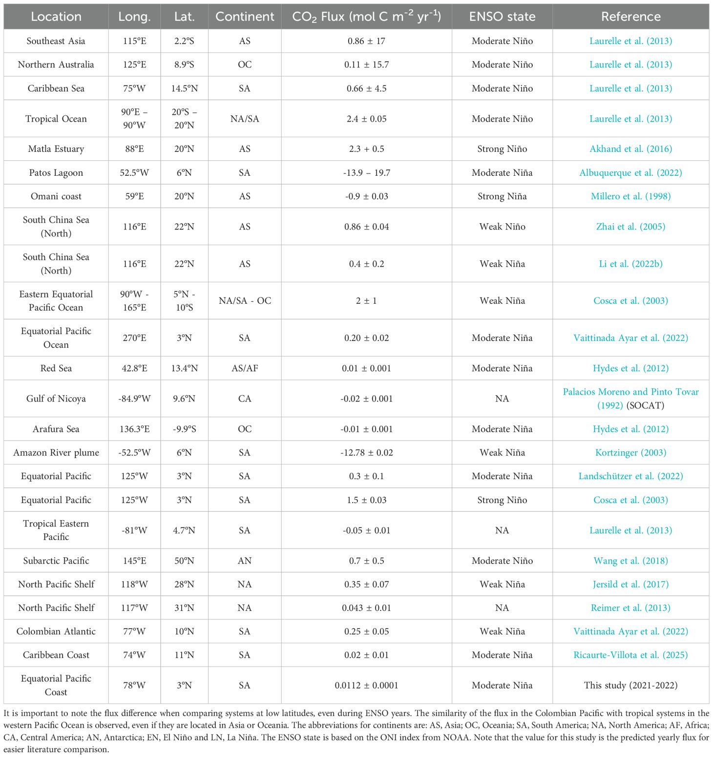
Table 1. CO₂ fluxes between air and sea in different geographic areas.

The Gorgona fluxes were also markedly lower than those observed in other tropical and coastal systems. For instance, at similar equatorial latitudes (~3°N), Jersild et al. (2017) and Landschützer et al. (2022) reported fluxes exceeding 0.3 ± 0.1 mol C m^-2 yr^-1 during moderate La Niña conditions. Pacific Ocean continental shelves exhibit values between 0.2 and 0.35 mol C m^-2 yr^-1 (Jersild et al., 2017; Vaittinada Ayar et al., 2022), while the North Pacific shelf, even under non-ENSO conditions, registers around 0.043 mol C m^-2 yr^-1 (Reimer et al., 2013). These regional differences suggest that local environmental controls strongly limit the air-sea CO₂ exchange in the Eastern Tropical Pacific, particularly near Gorgona. Consistent with this interpretation, Ricaurte-Villota et al. (2025) documented similarly low to near-neutral fluxes in the Colombian Caribbean under La Niña conditions, attributing them to high rainfall, enhanced stratification, and strong biological uptake. These drivers mirror those identified in our study, reinforcing the idea that La Niña exerts a suppressive effect on CO₂ release in this region. Comparable mechanisms have also been described in Arctic continental shelves, where freshwater inputs from rivers and ice melts (together with seasonal ice coverage) enhanced stratification, restricting gas exchange and contributing to low or near-neutral fluxes (Else et al., 2013; Miller et al., 2019; Mu et al., 2020).

Furthermore, comparison with other tropical systems reinforces our findings. Similar low or near-neutral fluxes have been reported in Costa Rica’s Gulf of Nicoya (Pfeil et al., 2013) and other areas of the Eastern Tropical Pacific (Laurelle et al., 2013).

Estuarine systems by contrast, tend to show higher fluxes and yearly variability (Chen et al., 2013). For example, the Matla estuary in India exhibits high annual fluxes of 2.3 mol C m^-2 yr^-1 (Akhand et al., 2016) over 10 times greater than the estimated CO₂ flux around Gorgona, and the Patos Lagoon in Brazil ranges from -13.9 to 19.7 mol C m^-2 yr^-1 attributed to changes in freshwater input and phytoplankton activity (Albuquerque et al., 2022). Meanwhile Asian tropical estuaries average around 8.1 mol C m^-2 yr^-1 (Chen et al., 2013) which are also substantially higher than our estimated yearly fluxes. However, comparable near-neutral fluxes were reported in the Arafura and Red Seas under similar La Niña conditions (Hydes et al., 2012).

Although global models (e.g., Dai et al., 2022) and some regional studies do not explicitly separate ENSO phases, this distinction is essential for accurately characterizing flux dynamics in equatorial regions such as Gorgona. Prior literature indicates that La Niña conditions can reduce FCO₂ by 0.2–0.4 mol C m^-2 yr^-1 in the Pacific region, compared to El Niño or neutral years, aligning with the low values observed in this study (Chavez et al., 1999; Landschützer et al., 2016; McKinley et al., 2020; Park et al., 2010).

Our findings challenge the assumption that upwelling-dominated systems and estuarine environment are high CO₂ emitters, especially under La Niña conditions. Since in our tropical coastal area FCO₂ is sensitive to atmospheric conditions (wind velocity, precipitation, solar radiation), freshwater discharge, physical dynamic (vertical-horizontal water movement), vertical stratification, upwelling events, carbonate chemistry and biological uptake. Future research should incorporate higher-resolution temporal data, uncertainty analyses in ΔpCO₂, and ENSO-phase-specific studies (and neutral/non-ENSO years) to improve carbon flux estimates in this and similar tropical estuarine systems.

4.7 Methodological considerations and recommendations

Our study did not include measurements of δ¹³C-DIC, which limits our ability to trace the biogeochemical sources and transformations of dissolved inorganic carbon. This isotopic parameter is a powerful tool for distinguishing between marine, terrestrial, and anthropogenic carbon inputs, and for assessing the extent of biological activity and remineralization. Its absence constrains our interpretation of carbon cycling dynamics, particularly under varying ENSO conditions. We suggest that future sampling campaigns incorporate δ¹³C-DIC analysis to enhance source attribution and improve the mechanistic understanding of CO₂ flux variability in coastal upwelling systems. Additionally, we did not directly measure nutrients, which limits our ability to consider them in the CO2SYS calculations, specifically those which are proton acceptors (e.g. phosphates, silicates, ammonia), which can have effects on the computation of certain carbonate system parameters under high nutrient loads. We recommend that future sampling efforts incorporate nutrient measurements for improved flux and carbonate system calculations.

It is important to consider methodological differences when comparing with other studies. Although references such as Feely et al. (2004, 2006) and Hydes et al. (2012) offer context, disparities in sampling protocols, spatial resolution, and ecosystem type limit the scope of direct comparison. Finally, we recommend a long-term monitoring program taking water samples to estimate in the lab the couple DIC/TA, this will allow to compare the CO₂ flux variability between ENSO events and neutral conditions. An inexpensive discrete sampling based on our experience for Gorgona National Park could be to take water samples for 2–4 contrasting months.

5 Conclusions

The estimated air-sea CO₂ flux at Gorgona Island (near 3°N in the Eastern Equatorial Pacific) was close to neutral (0.0104 mol C m^-2) during the nine sampled months under La Niña conditions. Gorgona displayed a bimodal regime: (I) a predominantly post-upwelling system for six months, characterized by slightly positive to near-neutral fluxes, augmented river discharge and rainfall, elevated sea surface temperatures (>27.4 °C), and high pCO_2W (567 μatm in average); and (II) three months of upwelling, with neutral or weakly negative fluxes (–0.1 ± 0.07 g C m^-2 day^-1), associated with CO₂ rich subsurface waters (nutrient rich) and phytoplankton uptake (minimum values of DeltaDIC aligned with the Chl-a maximum).

Although subsurface waters and coastal rivers deliver CO₂ to the surface, the intense and persistent stratification from low TA/DIC freshwater (high Revelle factor values; stratification starting at 10 to 45 m), reinforced by warmer surface waters, and freshwater downwelling, effectively limits CO₂ venting to the atmosphere. The estimated air-sea CO₂ flux at Gorgona Island aligns with global estimates proposed by Wong et al. (2022). Still is lower than those predicted by the model of Dai et al. (2022), suggesting the influence of local biogeochemical processes. In summary, under La Niña conditions, characterized by rainfall and river runoff (mean SSS = 29.5 ± 1.5) the combined effects of low wind speeds (<5 m s^-1), vertical stratification, and the biological activity appear to explain the net neutral balance in the air-sea CO₂ flux in this region. This study highlights the importance of integrating local physical and biological coastal processes (hydrography) when estimating region-specific CO₂ fluxes (in both magnitude and direction); additionally, long temporal in situ measurements under ENSO events such as El Niño and Neutral conditions are needed to compare with La Niña FCO₂ findings.

Nevertheless, the overall trend of low fluxes during La Niña, as shown across tropical estuaries and coastal systems, supports the hypothesis that this event suppresses CO₂ efflux through enhanced freshwater delivery and weakened ocean-atmosphere coupling. However, the hypothesis of high positive fluxes during El Niño or neutral years, when rainfall and upwelling are reduced at Gorgona, needs further investigation through seasonal and interannual monitoring campaigns including physical and biogeochemical variables.

Data availability statement

The datasets generated for this study can be found in the NOAA - National Centers for Environmental Information (NCEI; Accession Number 0300558). (NCEI; URL, https://www.ncei.noaa.gov/data/oceans/ncei/ocads/metadata/0300558.html).

Author contributions

SG: Writing – original draft, Formal analysis, Data curation, Writing – review & editing, Visualization, Software, Investigation, Validation, Methodology. AA: Conceptualization, Validation, Data curation, Supervision, Methodology, Project administration, Investigation, Resources, Writing – review & editing, Funding acquisition, Visualization, Formal analysis. AM: Methodology, Investigation, Visualization, Writing – review & editing. AG: Investigation, Data curation, Methodology, Writing – review & editing. AC-A: Conceptualization, Visualization, Writing – review & editing, Formal analysis. JH-A: Conceptualization, Writing – review & editing, Visualization. LC: Writing – review & editing, Validation, Methodology, Formal analysis, Visualization. LK: Visualization, Methodology, Formal analysis, Writing – review & editing. DR-P: Writing – review & editing, Supervision, Validation, Methodology.

Funding

The author(s) declare financial support was received for the research and/or publication of this article. The Principal Investigator (PI), AA, acknowledges receiving financial support for various research activities, including the purchase of equipment, acquisition of laboratory and field materials, and funding for field trips. Additionally, these funds were used to establish and equip a laboratory at the Pontificia Universidad Javeriana. Partial resources from the same fund were also allocated to cover the publication costs of this article (ID 21346). This research was funded by the National Geographic Explorer program through the project titled “Ocean Acidification Vulnerability in Colombia: First Monitoring Program in the Tropical Pacific” (Grant No. NGS-64756R-19), with additional COVID-19 grant support (Grant No. NGS-81727R-20). Further funding was provided by the Pontificia Universidad Javeriana under the project “Monitoreo de acidificación marina en el Pacífico colombiano” (Project ID: 120132C0401200, No. 20019; Grant ID 21347).

Acknowledgments

The Ocean Foundation donated the GOA-ON in a Box kit, OA training, and grant support for equipment maintenance under the Memorandum of Understanding between Pontificia Universidad Javeriana and The Ocean Foundation (“TOF”). This research is part of the collaboration with the International COCAS project (2021-2030), Ocean Decade-United Nations (Leader Diana Ruiz Pino and Alban Lazar) https://oceandecade.org/fr/actions/coastal-observatory-for-climate-co2-and-acidification-for-theglobal-south-society-cocas/. Dra. Andrea Corredor-Acosta thanks FONDECYT Postdoctoral Project No. 3230740 granted by the Chilean Agency for Research and Development (ANID). We also thank Parques Nacionales Naturales de Colombia - Gorgona for their logistical support at Gorgona (Christian Díaz – research head & Monitoring of the Gorgona park), accommodation and boat, and the research permit No. 004 de 2020 - file number: OTRP 004-2020. To Camilo, Freddy, and Jaime for their help in the Ocean Acidification laboratory. To Juan Felipe Cifuentes for his field assistance (monitoring) and also to Gabriela Cervantes Diaz for her help in the laboratory analysis at the UABC. Thanks to Dr. Alan Giraldo of Universidad del Valle for funding research interns Cristian Claros, Sebastián Ortiz, and Natalia Londoño, who collaborated with us in the field sampling. We thank Camilo Rodríguez and Enrique Herman for their help during the long days of boat sampling and for hosting us in their home during our stay at Guapi. Finally, a huge thanks to my friends, Hugo Barata, Catalina Infante, Iván Gonzales, Vinny Preiss, and my family, Mónica Duque, Juan Pablo Gutiérrez, and Emma Gutiérrez for their never-ending support, without which this research would not have been possible.

Conflict of interest

The authors declare that the research was conducted in the absence of any commercial or financial relationships that could be construed as a potential conflict of interest.

Generative AI statement

The author(s) declare that no Generative AI was used in the creation of this manuscript.

Any alternative text (alt text) provided alongside figures in this article has been generated by Frontiers with the support of artificial intelligence and reasonable efforts have been made to ensure accuracy, including review by the authors wherever possible. If you identify any issues, please contact us.

Publisher’s note

All claims expressed in this article are solely those of the authors and do not necessarily represent those of their affiliated organizations, or those of the publisher, the editors and the reviewers. Any product that may be evaluated in this article, or claim that may be made by its manufacturer, is not guaranteed or endorsed by the publisher.

Supplementary material

The Supplementary Material for this article can be found online at: https://www.frontiersin.org/articles/10.3389/fmars.2025.1633653/full#supplementary-material

References

Ahad J. M. E., Barth J. A. C., Ganeshram R. S., Spencer R. G. M., and Uher G. (2008). Controls on carbon cycling in two contrasting temperate zone estuaries: The Tyne and Tweed, UK. Estuarine. Coast. Shelf. Sci 78, 685–693. doi: 10.1016/j.ecss.2008.02.006

Crossref Full Text | Google Scholar

Akhand A., Chanda A., Manna S., Das S., Hazra S., Roy R., et al. (2016). A comparison of CO₂ dynamics and air-water fluxes in a river-dominated estuary and a mangrove-dominated marine estuary. Geophys. Res. Lett. 43. doi: 10.1002/2016gl070716

Crossref Full Text | Google Scholar

Albuquerque C., Kerr R., Monteiro T., MaChado E.da C., Carvalho A. da C.d., and Mendes C. R. B. (2022). Water-air exchanges in the lower estuary of the patos lagoon: seasonal variability, drivers, and sources of CO₂. doi: 10.21203/rs.3.rs-1336400/v1

Crossref Full Text | Google Scholar

Alldredge A. L. (1984). “The quantitative significance of gelatinous zooplankton as pelagic consumers,” In: Fasham M. J. R. (eds) Flows of Energy and Materials in Marine Ecosystems (Boston, MA: Springer US), 407–433. doi: 10.1007/978-1-4757-0387-0_16

Crossref Full Text | Google Scholar

Amaya C. A. A. (2024). “Las corrientes superficiales en la cuenca de Colombia observadas con boyas de deriva,” in Revisa de la Academia Colombiana de Ciencias Exactas, Físicas y Naturales, vol. 25. Bogotá, Colombia: Academia Colombiana de Ciencias Exactas, Físicas y Naturales (ACCEFYN), 321–336. doi: 10.18257/raccefyn.25(96).2001.2796

Crossref Full Text | Google Scholar

Amos C. M. and Castelao R. M. (2022). Influence of the El Niño-Southern oscillation on SST fronts along the west coasts of north and South America. J. Geophys. Res.: Oceans. 127. doi: 10.1029/2022JC018479

PubMed Abstract | Crossref Full Text | Google Scholar

Andersson A. J. (2005). Coastal ocean and carbonate systems in the high CO2 world of the Anthropocene. Am. J. Sci 305, 875–918. doi: 10.2475/ajs.305.9.875

Crossref Full Text | Google Scholar

Andersson A. J. and Gledhill D. (2013). Ocean acidification and coral reefs: effects on breakdown, dissolution, and net ecosystem calcification. Annu. Rev. Mar. Sci 5, 321–348. doi: 10.1146/annurev-marine-121211-172241

PubMed Abstract | Crossref Full Text | Google Scholar

Bakun A. and Nelson C. (1991). The seasonal cycle of wind-stress curl in subtropical eastern boundary current regions. J. Physical Oceanography 21 (12), 1815–1834. Available online at: https://journals.ametsoc.org/view/journals/phoc/21/12/1520-0485_1991_021_1815_tscows_2_0_co_2.xml

Google Scholar

Bouillon S. (2011). Storage beneath mangroves. Nature Geoscience 4 (5), 282–283. doi: 10.1038/ngeo1130

Crossref Full Text | Google Scholar

Blanco J. F. (2012). The hydroclimatology of Gorgona Island: seasonal and ENSO-related Patternsa. Actualidades. Biológicas. 31, 111–121. doi: 10.17533/udea.acbi.331494

Crossref Full Text | Google Scholar

Borges A. V. and Abril G. (2011). “Carbon dioxide and methane dynamics in estuaries,” in Treatise on Estuarine and Coastal Science (Elsevier), 119–161. doi: 10.1016/B978-0-12-374711-2.00504-0

Crossref Full Text | Google Scholar

Borges A. V., Delille B., and Frankignoulle M. (2005). Budgeting sinks and sources of CO₂ in the coastal ocean: Diversity of ecosystems counts. Geophys. Res. Lett. 32. doi: 10.1029/2005GL023053

Crossref Full Text | Google Scholar

Bravo L., Ramos M., Astudillo O., Dewitte B., and Goubanova K. (2016). Seasonal variability of the Ekman transport and pumping in the upwelling system off central-northern Chile (∼ 30° S) based on a high-resolution atmospheric regional model (WRF). Ocean. Sci 12, 1049–1065. doi: 10.5194/os-12-1049-2016

Crossref Full Text | Google Scholar

Cai W.-J. (2011). Estuarine and coastal ocean carbon paradox: CO 2 sinks or sites of terrestrial carbon incineration? Annu. Rev. Mar. Sci 3, 123–145. doi: 10.1146/annurev-marine-120709-142723

PubMed Abstract | Crossref Full Text | Google Scholar

Cai W.-J., Hu X., Huang W.-J., Murrell M. C., Lehrter J. C., Lohrenz S. E., et al. (2011). Acidification of subsurface coastal waters enhanced by eutrophication. Nat. Geosci. 4, 766–770. doi: 10.1038/ngeo1297

Crossref Full Text | Google Scholar

Cai W.-J. and Wang Y. (1998). The chemistry, fluxes, and sources of carbon dioxide in the estuarine waters of the Satilla and Altamaha Rivers, Georgia. Limnology and Oceanography 43 (4), 657–668. doi: 10.4319/lo.1998.43.4.0657

Crossref Full Text | Google Scholar

Chavez F. P., Service S. K., and Buttrey S. E. (1996). Temperature-nitrate relationships in the central and eastern tropical Pacific. J. Geophys. Res.: Oceans. 101, 20553–20563. doi: 10.1029/96JC01943

Crossref Full Text | Google Scholar

Chavez F. P., Strutton P. G., Friederich G. E., Feely R. A., Feldman G. C., Foley D. G., et al. (1999). Biological and chemical response of the equatorial pacific ocean to the 1997–98 El Niño. Science 286, 2126–2131. doi: 10.1126/science.286.5447.2126

PubMed Abstract | Crossref Full Text | Google Scholar

Chen C.-T. A. and Borges A. V. (2009). Reconciling opposing views on carbon cycling in the coastal ocean: Continental shelves as sinks and near-shore ecosystems as sources of atmospheric CO₂. Deep. Sea. Res. Part II.: Topical. Stud. Oceanogr. 56, 578–590. doi: 10.1016/j.dsr2.2009.01.001

Crossref Full Text | Google Scholar

Chen C., Huang T. S., Chen Y., Bai Y., He X.-T., and Kang Y.J. (2013). Air–sea exchanges of CO₂ in the world’s coastal seas. Biogeosciences 10, 6509–6544. doi: 10.5194/bg-10-6509-2013

Crossref Full Text | Google Scholar

Chung C. T. Y. and Power S. B. (2014). Precipitation response to La Niña and global warming in the Indo-Pacific. Climate Dynamics. 43, 3293–3307. doi: 10.1007/s00382-014-2105-9

Crossref Full Text | Google Scholar

Clark J. B., Uz S. S., Tsontos V., Huang T., Scott J., and Rogers L. (2022). Assessing carbon properties in coastal waters with a new observing system testbed. Oceans, 1–6. doi: 10.1109/OCEANS47191.2022.9977358

Crossref Full Text | Google Scholar

Corredor-Acosta A., Acosta A., Gaspar P., and Calmettes B. (2011). Variation in the surface currents in the Panama Bight during El Nino and LA Nina events from 1993 to 2007. Bull. Mar. Coast. Res. 40. doi: 10.25268/bimc.invemar.2011.40.0.127

Crossref Full Text | Google Scholar

Corredor-Acosta A., Cortés-Chong N., Acosta A., Pizarro-Koch M., Vargas A., Medellín-Mora J., et al. (2020). Spatio-temporal variability of chlorophyll-A and environmental variables in the Panama bight. Remote Sens. 12, 2150. doi: 10.3390/rs12132150

Crossref Full Text | Google Scholar

Cosca C. E., Feely R. A., Boutin J., Etcheto J., McPhaden M. J., Chavez F. P., et al. (2003). Seasonal and interannual CO₂ fluxes for the central and eastern equatorial Pacific Ocean as determined from fCO₂ -SST relationships. J. Geophys. Res.: Oceans. 108. doi: 10.1029/2000JC000677

Crossref Full Text | Google Scholar

Courtney T. A. and Andersson A. J. (2019). Evaluating measurements of coral reef net ecosystem calcification rates. Coral. Reefs. 38, 997–1006. doi: 10.1007/s00338-019-01828-2

Crossref Full Text | Google Scholar

Courtney T. A., Cyronak T., Griffin A. J., and Andersson A. J. (2021). Implications of salinity normalization of seawater total alkalinity in coral reef metabolism studies. PloS One 16, e0261210. doi: 10.1371/journal.pone.0261210

PubMed Abstract | Crossref Full Text | Google Scholar

Crawford G., Mepstead M., and Díaz-Ferguson E. (2023). Characterizing oceanographic conditions near Coiba Island and Pacific Panama using 20 years of satellite-based wind stress, SST and chlorophyll-a measurements. Mar. Fish. Sci. (MAFIS) 37, 391–411. doi: 10.47193/mafis.37X2024010112

Crossref Full Text | Google Scholar

Dai X., Ma J., Zhang H., and Xu W. (2013). Evaluation of ecosystem health for the coastal wetlands at the Yangtze Estuary, Shanghai. Wetlands. Ecol. Manage. 21, 433–445. doi: 10.1007/s11273-013-9316-4

Crossref Full Text | Google Scholar

Dai M., Su J., Zhao Y., Hofmann E. E., Cao Z., Cai W.-J., et al. (2022). Carbon fluxes in the coastal ocean: synthesis, boundary processes, and future trends. Annu. Rev. Earth Planet. Sci. 50, 593–626. doi: 10.1146/annurev-earth-032320-090746

Crossref Full Text | Google Scholar

DeGrandpre M. D., Hammar T. R., and Wirick C. D. (1998). Short-term pCO₂ and O₂ dynamics in California coastal waters. Deep. Sea. Res. Part II.: Topical. Stud. Oceanogr. 45, 1557–1575. doi: 10.1016/S0967-0645(98)80006-4

Crossref Full Text | Google Scholar

Devis-Morales A., Schneider W., Montoya-Sánchez R. A., and Rodríguez Rubio E. (2008). Monsoon-like winds reverse oceanic circulation in the Panama Bight. Geophys. Res. Lett. 35, L20607. doi: 10.1029/2008GL035172

Crossref Full Text | Google Scholar

Diaz R. J. (2001). Overview of hypoxia around the world. J. Environ. Qual. 30, 275–281. doi: 10.2134/jeq2001.302275x

PubMed Abstract | Crossref Full Text | Google Scholar

Díaz Guevara D. C., Málikov I., and Villegas Bolaños N. L. (2008). Características de las zonas de surgencia de la cuenca del Pacífico Colombiano y su relación con la zona de convergencia intertropical. Boletín. Científico. CIOH. 26, 59–71. doi: 10.26640/01200542.26.59_71

Crossref Full Text | Google Scholar

Dickson A. G. (1990). Standard potential of the reaction: AgCl (s)+ 12H2 (g)= Ag (s)+ HCl (aq), and the standard acidity constant of the ion HSO₄– in synthetic sea water from 273.15 to 318.15 K. J. Chem. Thermodynamics. 22, 113–127. doi: 10.1016/0021-9614(90)90074-z

Crossref Full Text | Google Scholar

Dickson A. G., Sabine C. L., and Christian J. R. (Eds.) (2007). Guide to best practices for ocean CO₂ measurements (PICES Special Publication 3), 191. (“Guide” in one PDF file). Available online at: https://www.ncei.noaa.gov/access/ocean-carbon-acidification-data-system/oceans/Handbook_2007/Guide_all_in_one.pdf

Google Scholar

Doney S. C., Lima I., Feely R. A., Glover D. M., Lindsay K., Mahowald N., et al. (2009b). Mechanisms governing interannual variability in upper-ocean inorganic carbon system and air–sea CO₂ fluxes: Physical climate and atmospheric dust. Deep. Sea. Res. Part II.: Topical. Stud. Oceanogr. 56, 640–655. doi: 10.1016/j.dsr2.2008.12.006

Crossref Full Text | Google Scholar

Else B. G. T., Papakyriakou T. N., Galley R. J., Mucci A., Gosselin M., Miller L. A., et al. (2013). Annual cycle of air–sea CO₂ exchange in an Arctic Polynya region. J. Geophys. Res.: Biogeosci. 118, 681–703. doi: 10.1002/jgrg.20023

Crossref Full Text | Google Scholar

Engel A., Kiko R., and Dengler M. (2022). Organic matter supply and utilization in oxygen minimum zones. Annu. Rev. Mar. Sci 14, 355–378. doi: 10.1146/annurev-marine-041921-090849

PubMed Abstract | Crossref Full Text | Google Scholar

Fabre C., Sauvage S., Probst J.-L., and Sánchez-Pérez J. M. (2020). Global-scale daily riverine DOC fluxes from lands to the oceans with a generic model. Global and Planetary Change 194, 103294. doi: 10.1016/j.gloplacha.2020.103294

Crossref Full Text | Google Scholar

Feely R., Doney S., and Cooley S. (2009). Ocean acidification: present conditions and future changes in a high-CO₂ world. Oceanography 22, 36–47. doi: 10.5670/oceanog.2009.95

Crossref Full Text | Google Scholar

Feely R. A., Takahashi T., Wanninkhof R., McPhaden M. J., Cosca C. E., Sutherland S. C., et al. (2006). Decadal variability of the air-sea CO₂ fluxes in the equatorial Pacific Ocean. J. Geophys. Res.: Oceans. 111. doi: 10.1029/2005JC003129

Crossref Full Text | Google Scholar

Feely R. A., Wanninkhof R., McGillis W., Carr M.-E., and Cosca C. E. (2004). Effects of wind speed and gas exchange parameterizations on the air-sea CO₂ fluxes in the equatorial Pacific Ocean. J. Geophys. Res.: Oceans. 109. doi: 10.1029/2003JC001896

Crossref Full Text | Google Scholar

Fiedler P. C. and Lavín M. F. (2017). Oceanographic Conditions of the Eastern Tropical Pacific. Berlin: Springer Nature Link 59–83. doi: 10.1007/978-94-017-7499-4_3

Crossref Full Text | Google Scholar

Ford D. J., Tilstone G. H., Shutler J. D., and Kitidis V. (2022). Identifying the biological control of the annual and multi-year variations in South Atlantic air–sea CO₂ flux. Biogeosciences 19, 4287–4304. doi: 10.5194/bg-19-4287-2022

Crossref Full Text | Google Scholar

Friedlingstein P., O’Sullivan M., Jones M. W., Andrew R. M., Bakker D. C. E., Hauck J., et al. (2023). Global carbon budget 2023. Earth Syst. Sci Data 15, 5301–5369. doi: 10.5194/essd-15-5301-2023

Crossref Full Text | Google Scholar

Gan J., Li L., Wang D., and Guo X. (2009). Interaction of a river plume with coastal upwelling in the northeastern South China Sea. Continent. Shelf. Res. 29, 728–740. doi: 10.1016/j.csr.2008.12.002

Crossref Full Text | Google Scholar

Gassen L., Esters L., Ribas-Ribas M., and Wurl O. (2024). The impact of rainfall on the sea surface salinity: a mesocosm study. Sci. Rep. 14, 6353. doi: 10.1038/s41598-024-56915-4

PubMed Abstract | Crossref Full Text | Google Scholar

Gerrard M. B. (2023). “The role of ocean CDR in mitigating climate change,” in Ocean Carbon Dioxide Removal for Climate Mitigation (Edward Elgar Publishing), 12–19. doi: 10.4337/9781802208856.00009

Crossref Full Text | Google Scholar

Giraldo A., Rodríguez-Rubio E., and Zapata F. (2008). Condiciones oceanográficas en isla Gorgona, Pacífico oriental tropical de Colombia. Latin. Am. J. Aquat. Res. 36, 121–128. doi: 10.3856/vol36-issue1-fulltext-12

Crossref Full Text | Google Scholar

Giraldo A., Valencia B., and Ramírez D. G. (2011). Productividad planctónica y condiciones oceanográficas locales en Isla Gorgona durante julio 2006. Bol. Invest. Mar. Cost. 40, 185–201. doi: 10.25268/bimc.invemar.2011.40.1.108

Crossref Full Text | Google Scholar

Giraldo López A. (2008). Variabilidad espacial de temperatura, salinidad y transparencia en el ambiente pelágico del PNN Gorgona durante septiembre 2007 y marzo 2008. Boletín. Científico. CIOH. 26, 157–163. doi: 10.26640/22159045.192

Crossref Full Text | Google Scholar

Guzmán D. H., Mier R. L., Vergara A., and Milanes C. B. (2023). Marine protected areas in Colombia: A historical review of legal marine protection since the late 1960s to 2023. Marine Policy, 155, 105726. doi: 10.1016/j.marpol.2023.105726

Crossref Full Text | Google Scholar

Hans-Rolf D. and Fritz V. (2023). Oceans’ surface pH-value as an example of a reversible natural response to an anthropogenic perturbation. Ann. Mar. Sci 7, 034–039. doi: 10.17352/ams.000036

Crossref Full Text | Google Scholar

Herrera Carmona J. C., Selvaraj J. J., and Giraldo A. (2022). Dynamic regionalization of the Panama Bight, Eastern Tropical Pacific, using remote sensing data. Int. J. Remote Sens. 43, 3131–3151. doi: 10.1080/01431161.2022.2063040

Crossref Full Text | Google Scholar

Hu J., Lan W., Huang B., Chiang K.-P., and Hong H. (2015). Low nutrient and high chlorophyll a coastal upwelling system – A case study in the southern Taiwan Strait. Estuarine. Coast. Shelf. Sci 166, 170–177. doi: 10.1016/j.ecss.2015.05.020

Crossref Full Text | Google Scholar

Huang J., Li Q., Wu P., Wang S., Gu S., Guo M., et al. (2022). The buffering of a riverine carbonate system under the input of acid mine drainage: Example from a small karst watershed, southwest China. Front. Environ. Sci. 10 doi: 10.3389/fenvs.2022.1020452

Crossref Full Text | Google Scholar

Hydes D., Jiang Z.-P., Hartman M. C., Campbell J. M., Hartman S. E., Pagnani M. R., et al. (2012). Surface DIC and TALK measurements along the M/V Pacific Celebes VOS Line during the 2007–2012 cruises. Carbon Dioxide Information Analysis Center, Oak Ridge National Laboratory, US Department of Energy, Oak Ridge, TN. doi: 10.3334/CDIAC/OTG.VOS_PC_2007-2012

Crossref Full Text | Google Scholar

Ianson D., Feely R. A., Sabine C. L., and Juranek L. W. (2009). Features of coastal upwelling regions that determine net air-sea CO₂ flux. J. Oceanogr. 65, 677–687. doi: 10.1007/s10872-009-0059-z

Crossref Full Text | Google Scholar

INVEMAR. (2019). Informe del Estado de los Ambientes Marinos y Costeros en Colombia 2019 (Santa Marta: Instituto de Investigaciones Marinas y Costeras INVEMAR). Available online at: https://portal.invemar.org.co/inf-ier (Accessed July 28, 2023).

Google Scholar

INVEMAR. (2020). Informe del Estado de los Ambientes Marinos y Costeros en Colombia 2020 (Santa Marta: Instituto de Investigaciones Marinas y Costeras INVEMAR). Available online at: https://portal.invemar.org.co/inf-ier (Accessed July 28, 2023).

Google Scholar

INVEMAR. (2022). Informe del Estado de los Ambientes Marinos y Costeros en Colombia 2022 (Santa Marta: Instituto de Investigaciones Marinas y Costeras INVEMAR). Available online at: https://portal.invemar.org.co/inf-ier (Accessed July 28, 2023).

Google Scholar

Jersild A., Landschützer P., Gruber N., and Bakker D. C. E. (2017). An observation-based global monthly gridded sea surface pCO₂ and air–sea CO₂ flux product from 1982 onward (NCEI Accession 0160558). NOAA National Centers for Environmental Information. doi: 10.7289/V5Z899N6

Crossref Full Text | Google Scholar

Jiang Z.-P., Tyrrell T., Hydes D. J., Dai M., and Hartman S. E. (2014). Variability of alkalinity and the alkalinity-salinity relationship in the tropical and subtropical surface ocean, Global Biogeochem. Cycles 28, 729–742. doi: 10.1002/2013GB004678

Crossref Full Text | Google Scholar

Johnson M. S., Billett M. F., Dinsmore K. J., Wallin M., Dyson K. E., and Jassal R. S. (2010). Direct and continuous measurement of dissolved carbon dioxide in freshwater aquatic systems—method and applications. Ecohydrology 3, 68–78. doi: 10.1002/eco.95

Crossref Full Text | Google Scholar

Johnson K., Sieburth J. M., Williams P.J. le., and Brändström L. (1987). Coulometric total carbon dioxide analysis for marine studies: Automation and calibration. Mar. Chem. 21, 117–133. doi: 10.1016/0304-4203(87)90033-8

Crossref Full Text | Google Scholar

Kahl L. C. (2018). Dinámica del CO₂ en el Océano Atlántico Sudoccidental (Buenos Aires, Argentina: Universidad de Buenos Aires, Facultad de Ciencias Exactas y Naturales). Available online at: https://hdl.handle.net/20.500.12110/tesis_n6525_Kahl (Accessed May 17, 2025).

Google Scholar

Kao H.-Y. and Yu J.-Y. (2009). Contrasting eastern-pacific and central-pacific types of ENSO. J. Climate 22, 615–632. doi: 10.1175/2008jcli2309.1

Crossref Full Text | Google Scholar

Kawabe M. and Fujio S. (2010). Pacific Ocean circulation based on observation. J. Oceanogr. 66, 389–403. doi: 10.1007/s10872-010-0034-8

Crossref Full Text | Google Scholar

Kessler W. S. (2006). The circulation of the eastern tropical Pacific: A review. Prog. Oceanogr. 69, 181–217. doi: 10.1016/j.pocean.2006.03.009

Crossref Full Text | Google Scholar

Kim D., Choi Y., Kim T.-W., and Park G.-H. (2017). Recent increase in surface fCO₂ in the western subtropical North Pacific. Ocean. Sci J. 52, 329–335. doi: 10.1007/s12601-017-0030-7

Crossref Full Text | Google Scholar

Kim H. J., Kim T., Hyeong K., Yeh S., Park J., Yoo C. M., et al. (2019). Suppressed CO₂ outgassing by an enhanced biological pump in the eastern tropical pacific. J. Geophys. Res.: Oceans. 124, 7962–7973. doi: 10.1029/2019JC015287

Crossref Full Text | Google Scholar

Körtzinger A. (2003). A significant CO2 sink in the tropical Atlantic Ocean associated with the Amazon River plume. Geophysical Research Letters 30 (24), 2287. doi: 10.1029/2003GL018841

Crossref Full Text | Google Scholar

Kryzhova K. A. and Semkin P. Y. (2023). Carbonate System and CO₂ Fluxes in the Partizanskaya River Estuary. Berlin: Springer Nature Link 268–279. doi: 10.1007/978-3-031-47851-2_32

Crossref Full Text | Google Scholar

Lal R. B. (2024). Recent trends in carbon sequestration technique. J. Biochemical Sciences. doi: 10.61577/jbs.2024.100003

Crossref Full Text | Google Scholar

Landschützer P., Gruber N., and Bakker D. C. E. (2016). Decadal variations and trends of the global ocean carbon sink. Global Biogeochem. Cycles. 30, 1396–1417. doi: 10.1002/2015GB005359

Crossref Full Text | Google Scholar

Landschützer P., Keppler L., and Ilyina T. (2022). Ocean systems (Elsevier eBooks), 427–452. doi: 10.1016/b978-0-12-814952-2.00004-6

Crossref Full Text | Google Scholar

Lanson D., Feely R. A., Sabine C. L., and Juranek L. W. (2009). Features of coastal upwelling regions that determine net air–sea CO2 flux. J. Oceanography 65 (5), 677–687. doi: 10.1007/s10872-009-0059-z

Crossref Full Text | Google Scholar

Laruelle G. G., Dürr H. H., Slomp C. P., Borges A. V., Gypens N., Lauerwald R., et al. (2013). Air–sea CO2 exchanges in the world’s coastal seas. Biogeosciences 10, 6509–6544. doi: 10.5194/bg-10-6509-2013

Crossref Full Text | Google Scholar

Lee K., Kim T. W., Byrne R. H., Millero F. J., Feely R. A., and Liu Y. M. (2010). The universal ratio of boron to chlorinity for the North Pacific and North Atlantic oceans. Geochim. Cosmochim. Acta 74, 1801–1811. doi: 10.1016/j.gca.2009.12.027

Crossref Full Text | Google Scholar

Legge O. J., Bakker D. C. E., Johnson M. T., Meredith M. P., Venables H. J., Brown P. J., et al. (2015). The seasonal cycle of ocean-atmosphere CO₂ flux in Ryder Bay, west Antarctic Peninsula. Geophys. Res. Lett. 42, 2934–2942. doi: 10.1002/2015GL063796

Crossref Full Text | Google Scholar

Lewis E. and Wallace (1998). Program Developed for CO₂ System Calculations OSTI OAI (U.S. Department of Energy Office of Scientific and Technical Information). doi: 10.15485/1464255

Crossref Full Text | Google Scholar

Li J., Cao R., Lao Q., Chen F., Chen C., Zhou X., et al. (2020). Assessing seasonal nitrate contamination by nitrate dual isotopes in a monsoon-controlled bay with intensive human activities in South China. Int. J. Environ. Res. Public Health 17, 1921. doi: 10.3390/ijerph17061921

PubMed Abstract | Crossref Full Text | Google Scholar

Li H., Zhang J., Xuan J., Wu Z., Ran L., Wiesner M. G., et al. (2022). Asymmetric response of the biological carbon pump to the ENSO in the south China sea. Geophys. Res. Lett. 49. doi: 10.1029/2021gl095254

Crossref Full Text | Google Scholar

Liss P. S. and Merlivat L. (1986). Air–sea gas exchange rates: Introduction and synthesis, in Buat-Ménard P. (ed.), The Role of Air–Sea Exchange in Geochemical Cycling, NATO ASI Series (Series C: Mathematical and Physical Sciences), vol. 185, Springer, Dordrecht, 113–127. doi: 10.1007/978-94-009-4738-2_5

Crossref Full Text | Google Scholar

Lorenzoni L., Hu C., Varela R., Arias G., Guzmán L., and Muller-Karger F. (2011). Bio-optical characteristics of Cariaco Basin (Caribbean Sea) waters. Continent. Shelf. Res. 31, 582–593. doi: 10.1016/j.csr.2010.12.013

Crossref Full Text | Google Scholar

Macdonald H. S., Baird M. E., and Middleton J. H. (2009). Effect of wind on continental shelf carbon fluxes off southeast Australia: A numerical model. J. Geophys. Res.: Oceans. 114. doi: 10.1029/2008JC004946

Crossref Full Text | Google Scholar

McKee B. A., Aller R. C., Allison M. A., Bianchi T. S., and Kineke G. C. (2004). Transport and transformation of dissolved and particulate materials on continental margins influenced by major rivers: benthic boundary layer and seabed processes. Continent. Shelf. Res. 24, 899–926. doi: 10.1016/j.csr.2004.02.009

Crossref Full Text | Google Scholar

McKinley G. A., Fay A. R., Eddebbar Y. A., Gloege L., and Lovenduski N. S. (2020). External forcing explains recent decadal variability of the ocean carbon sink. AGU. Adv. 1. doi: 10.1029/2019AV000149

Crossref Full Text | Google Scholar

McLean P., Bulmer C., Davies P., Dunstone N., Gordon M., Ineson S., et al. (2024). Predictability of European winter 2021/2022: Influence of La Niña and stratospheric polar vortex. Atmospher. Sci Lett. 25. doi: 10.1002/asl.1255

Crossref Full Text | Google Scholar

Miller L. A., Shadwick E. H., and Thomas H. (2019). Air–sea CO₂ fluxes in the Hudson Bay system: The role of stratification. Geophys. Res. Lett. 46, 541–549. doi: 10.1029/2018GL080099

Crossref Full Text | Google Scholar

Millero F. J. (2010). Carbonate constants for estuarine waters. Mar. Freshw. Res. 61, 139–142. doi: 10.1071/mf09254

Crossref Full Text | Google Scholar

Millero F. J., Degler E. A., O’Sullivan D. W., Goyet C., and Eischeid G. (1998). The carbon dioxide system in the Arabian Sea. Deep Sea Research Part II 45, 2225–2252.

Google Scholar

Millero F. J., Lee K., and Roche M. P. (1998). Distribution of alkalinity in the surface waters of the major oceans. Marine Chemistry 60 (1–2), 111–130. doi: 10.1016/S0304-4203(97)00084-4

Crossref Full Text | Google Scholar

Monteiro T., Batista M., Henley S., MaChado E., da C., Araujo M., et al. (2022). Contrasting sea-air CO₂ exchanges in the western tropical atlantic ocean. Global Biogeochem. Cycles. 36. doi: 10.1029/2022GB007385

Crossref Full Text | Google Scholar

Mu L., Gruber N., and Doney S. C. (2020). Seasonality of air–sea CO₂ fluxes in the Arctic Ocean: The role of sea ice, freshwater input, and biological uptake. Global Biogeochem. Cycles. 34, e2020GB006574. doi: 10.1029/2020GB006574

Crossref Full Text | Google Scholar

Murcia Riaño M. and Giraldo López A. (2007). Condiciones oceanográficas y composición del Mesozooplancton en la zona oceánica del Pacífico Colombiano, durante septiembre-octubre 2004. Boletín. Científico. CCCP. 14, 83–94. doi: 10.26640/01213423.14.83_94

Crossref Full Text | Google Scholar

NOAA. (2021). Mauna Loa CO₂ monthly mean data. NOAA Global Monitoring Laboratory. Available online at: https://gml.noaa.gov/ccgg/trends/data.html (Accessed September 2022)

Google Scholar

NOAA. (2022). Mauna Loa CO₂ monthly mean data. NOAA Global Monitoring Laboratory. Available online at: https://gml.noaa.gov/ccgg/trends/data.html (Accessed September 2022)

Google Scholar

Olafsson J., Olafsdottir S. R., Takahashi T., Danielsen M., and Arnarson T. S. (2021). Enhancement of the north atlantic CO₂ sink by arctic waters. Biogeosciences 18, 1689–1701. doi: 10.5194/bg-18-1689-2021

Crossref Full Text | Google Scholar

Oliveira A. P., Fernandes A. M., Fonseca V. F., Vale C., and Mendonça A. M. M. (2017). Inorganic carbon distribution and CO₂ fluxes in a large tropical estuary (Tagus, Portugal). Scientific Reports. doi: 10.1038/s41598-017-06758-z

PubMed Abstract | Crossref Full Text | Google Scholar

Palacios Moreno M. A. and Pinto Tovar C. A. (1992). Estudio de la influencia de la marea en el río Guapi. Boletín. Científico. CCCP. 3, 3–13. doi: 10.26640/01213423.3.3_13

Crossref Full Text | Google Scholar

Palacios Peñaranda M. L., Cantera Kintz J. R., and Peña Salamanca E. J. (2019). Carbon stocks in mangrove forests of the Colombian Pacific. Estuarine. Coast. Shelf. Sci 227, 106299. doi: 10.1016/j.ecss.2019.106299

Crossref Full Text | Google Scholar

Park G.-H., Wanninkhof R., Doney S. C., Takahashi T., Lee K., Feely R. A., et al. (2010). Variability of global net sea air CO₂; fluxes over the last three decades using empirical relationships. Tellus. B.: Chem. Phys. Meteorol. 62, 352. doi: 10.1111/j.1600-0889.2010.00498.x

Crossref Full Text | Google Scholar

Parv S., Chen Z., Shutler J., and Watson A.. (2023). Assessing Air–sea CO2 flux products with constraints from atmospheric inverse analyses. EGU General Assembly 2023. doi: 10.5194/egusphere-egu23-10224

Crossref Full Text | Google Scholar

Pasquero C., Bracco A., and Provenzale A. (2005). Impact of the spatiotemporal variability of the nutrient flux on primary productivity in the ocean. J. Geophys. Res.: Oceans. 110. doi: 10.1029/2004JC002738

Crossref Full Text | Google Scholar

Paulmier A., Ruiz-Pino D., and Garçon V. (2011). CO₂ maximum in the oxygen minimum zone (OMZ). Biogeosciences 8, pp.239–pp.252. doi: 10.5194/bg-8-239-2011

Crossref Full Text | Google Scholar

Peng C., Crawshaw J. P., Maitland G. C., Martin Trusler J. P., and Vega-Maza D. (2013). The pH of CO₂-saturated water at temperatures between 308K and 423K at pressures up to 15MPa. J. Supercrit. Fluids. 82, 129–137. doi: 10.1016/j.supflu.2013.07.001

Crossref Full Text | Google Scholar

Perez F. F. and Fraga F. (2003). Association constant of fluoride and hydrogen ions in seawater. Mar. Chem. 21, 161–168. doi: 10.1016/0304-4203(87)90036-3

Crossref Full Text | Google Scholar

Pierrot D., Epitalon J.-M., Orr J. C., and Lewis E. R. (2021). and Wallace, D.: MS Excel program developed for CO₂ system calculations – version 3.0. Available online at: https://github.com/dpierrot/co2sys_xl (Accessed May 17, 2025).

Google Scholar

Polavarapu S. M., Deng F., Byrne B., Jones D. B. A., and Neish M. (2018). A comparison of atmospheric CO2 flux signals obtained from GEOS-Chem flux inversions constrained by in situ or GOSAT observations. doi: 10.5194/acp-2017-1235

Crossref Full Text | Google Scholar

Prytherch J., Yelland M. J., Pascal R. W., Moat B. I., Skjelvan I., and Srokosz M. A. (2010). Open ocean gas transfer velocity derived from long-term direct measurements of the CO₂ flux. Geophys. Res. Lett. 37. doi: 10.1029/2010GL045597

Crossref Full Text | Google Scholar

Quiñones-Rivera Z. J., Wissel B., Turner R. E., Rabalais N. N., Justić D., Finlay K. P., et al. (2022). Divergent effects of biological and physical processes on dissolved oxygen and dissolved inorganic carbon dynamics on a eutrophied and hypoxic continental shelf. Limnol. Oceanogr. 67, 2603–2616. doi: 10.1002/lno.12225

Crossref Full Text | Google Scholar

Ramaekers L., Vanschoenwinkel B., Brendonck L., and Pinceel T. (2023). Elevated dissolved carbon dioxide and associated acidification delays maturation and decreases calcification and survival in the freshwater crustacean Daphnia magna. Limnol. Oceanogr. 68, 1624–1635. doi: 10.1002/lno.12372

Crossref Full Text | Google Scholar

Rastogi B., Miller J. B., Trudeau M., Andrews A. E., Hu L., Mountain M., et al. (2021). Evaluating consistency between total column CO2 retrievals from OCO-2 and the in situ network over North America: implications for carbon flux estimation. Atmospheric Chemistry and Physics 21 (18), 14385–14401. doi: 10.5194/acp-21-14385-2021

Crossref Full Text | Google Scholar

Reimer J. J., Vargas R., Smith S. V., Lara-Lara R., Gaxiola-Castro G., Martín Hernández-Ayón J., et al. (2013). Air-sea CO₂ fluxes in the near-shore and intertidal zones influenced by the California Current. J. Geophys. Res.: Oceans. 118, 4795–4810. doi: 10.1002/jgrc.20319

Crossref Full Text | Google Scholar

Restrepo J. D. and Kjerfve B. (2004). “The pacific and caribbean rivers of Colombia: water discharge, sediment transport and dissolved loads,” in Environmental Geochemistry in Tropical and Subtropical Environments (Springer Berlin Heidelberg), 169–187. doi: 10.1007/978-3-662-07060-4_14

Crossref Full Text | Google Scholar

Ricaurte-Villota C., Murcia-Riaño M., and Hernádez-Ayón J. M. (2025). Dynamics and drivers of the carbonate system: response to terrestrial runoff and upwelling along the Northeastern Colombian Caribbean coast. Front. Mar. Sci 11. doi: 10.3389/fmars.2024.1305542

Crossref Full Text | Google Scholar

Ries J. B., Cohen A. L., and McCorkle D. C. (2009). Marine calcifiers exhibit mixed responses to CO₂-induced Ocean acidification. Geology 37, 1131–1134. doi: 10.1130/G30210A.1

Crossref Full Text | Google Scholar

Rodríguez-Rubio E., Schneider W., and Abarca del Río R. (2003). On the seasonal circulation within the Panama Bight derived from satellite observations of wind, altimetry and sea surface temperature. Geophys. Res. Lett. 30. doi: 10.1029/2002GL016794

Crossref Full Text | Google Scholar

Roobaert A., Goulven L., Resplandy L., Landschützer P., Gruber N., Liao E., et al. (2021). The spatiotemporal dynamics of the sources and sinks of CO2 in the global coastal ocean. MPG.PuRe (Max Planck Society). doi: 10.5194/egusphere-egu21-10048

Crossref Full Text | Google Scholar

Roobaert A., Regnier P., Landschützer P., and Laruelle G. G. (2024). A novel sea surface pCO₂-product for the global coastal ocean resolving trends over 1982–2020. Earth Syst. Sci Data 16, 421–441. doi: 10.5194/essd-16-421-2024

Crossref Full Text | Google Scholar

Roobaert A., Regnier P., Landschützer P., and Laruelle G. G. (2025). Global coastal ocean CO₂ trends over the 1982–2020 period. doi: 10.5194/egusphere-egu24-14775

Crossref Full Text | Google Scholar

Rosentreter J. A., Laruelle G. G., Bange H. W., Bianchi T. S., Busecke J. J. M., Cai W.-J., et al. (2023). Coastal vegetation and estuaries are collectively a greenhouse gas sink. Nat. Climate Change 13, 579–587. doi: 10.1038/s41558-023-01682-9

Crossref Full Text | Google Scholar

Santos I. R., Hatje V., Serrano O., Bastviken D., and Krause-Jensen D. (2022). Carbon sequestration in aquatic ecosystems: Recent advances and challenges. Limnol. Oceanogr. 67. doi: 10.1002/lno.12268

Crossref Full Text | Google Scholar

Saraswat R. (2011). “Global equatorial sea-surface temperatures over the last 150,000 years: an update from foraminiferal elemental analysis,” in current science, vol. 100. Bangalore, India: Current Science, 1201–1206.

Google Scholar

Schneider T., Bischoff T., and Haug G. H. (2014). Migrations and dynamics of the intertropical convergence zone. Nature 513, 45–53. doi: 10.1038/nature13636

PubMed Abstract | Crossref Full Text | Google Scholar

Séférian R., Bopp L., Swingedouw D., and Servonnat J. (2013). Dynamical and biogeochemical control on the decadal variability of ocean carbon fluxes. Earth Syst. Dynamics. 4, 109–127. doi: 10.5194/esd-4-109-2013

Crossref Full Text | Google Scholar

Smith S. V. and Hollibaugh J. T. (1993). Coastal metabolism and the oceanic organic carbon balance. Rev. Geophys. 31, 75–89. doi: 10.1029/92RG02584

Crossref Full Text | Google Scholar

Stevenson M. (1970). Circulation in the Panama bight. J. Geophys. Res. 75, 659–672. doi: 10.1029/JC075i003p00659

Crossref Full Text | Google Scholar

Strutton P. G., Evans W., and Chavez F. P. (2008). Equatorial Pacific chemical and biological variability 1997–2003. Global Biogeochem. Cycles. 22. doi: 10.1029/2007GB003045

Crossref Full Text | Google Scholar

Sun Q., Li D., Wang B., Xu Z., Miao Y., Lin H., et al. (2023). Massive nutrients offshore transport off the Changjiang Estuary in flooding summer of 2020. Front. Mar. Sci 10. doi: 10.3389/fmars.2023.1076336

Crossref Full Text | Google Scholar

Swesi A., Yusup Y., Ahmad M. I., Almdhun H. M., Jamshidi E. J., Sigid M. F., et al. (2023). Seasonal and yearly controls of CO₂ fluxes in a tropical coastal ocean. Earth Interact. 27. doi: 10.1175/EI-D-22-0023.1

Crossref Full Text | Google Scholar

Takahashi T., Feely R. A., Weiss R. F., Wanninkhof R. H., Chipman D. W., Sutherland S. C., et al. (1997). Global air-sea flux of CO₂: An estimate based on measurements of sea–air pCO₂ difference. Proc. Natl. Acad. Sci. 94, 8292–8299. doi: 10.1073/pnas.94.16.8292

PubMed Abstract | Crossref Full Text | Google Scholar

Takahashi T., Sutherland S. C., Sweeney C., Poisson A., Metzl N., Tilbrook B., et al. (2002). Global sea–air CO₂ flux based on climatological surface ocean pCO₂, and seasonal biological and temperature effects. Deep. Sea. Res. Part II.: Topical. Stud. Oceanogr. 49, 1601–1622. doi: 10.1016/S0967-0645(02)00003-6

Crossref Full Text | Google Scholar

Tide-Forecast.com (2022). Map of tide Stations in Colombia. Available online at: https://www.tide-forecast.com/weather_maps/Colombia (Accessed May 17, 2025).

Google Scholar

Tomczak M. (1981). A multi-parameter extension of temperature/salinity diagram techniques for the analysis of non-isopycnal mixing. Prog. Oceanogr. 10, 147–171. doi: 10.1016/0079-6611(81)90010-0

Crossref Full Text | Google Scholar

Torres R. R., Giraldo E., Muñoz C., Caicedo A., Hernández-Carrasco I., and Orfila A. (2023). Seasonal and El Niño–Southern oscillation-related ocean variability in the Panama bight. Ocean. Sci 19, 685–701. doi: 10.5194/os-19-685-2023

Crossref Full Text | Google Scholar

UAESPNN (2005). Parque Nacional Natural Gorgona: Plan de Manejo 2005–2009 (Cali: Unidad Administrativa Especial del Sistema de Parques Nacionales Naturales de Colombia). Available online at: https://koha.parquesnacionales.gov.co/cgi-bin/koha/opac-detail.pl?biblionumber=3899 (Accessed May 17, 2025).

Google Scholar

Vaittinada Ayar P., Bopp L., Christian J. R., Ilyina T., Krasting J. P., Séférian R., et al. (2022). Contrasting projections of the ENSO-driven CO₂ flux variability in the equatorial Pacific under high-warming scenario. Earth Syst. Dynamics. 13, 1097–1118. doi: 10.5194/esd-13-1097-2022

Crossref Full Text | Google Scholar

Vargas C. A., Martínez R. A., Cuevas L. A., Pavez M. A., Cartes C., GonzÁlez H. E., et al. (2007). The relative importance of microbial and classical food webs in a highly productive coastal upwelling area. Limnol. Oceanogr. 52, 1495–1510. doi: 10.4319/lo.2007.52.4.1495

Crossref Full Text | Google Scholar

Wang D., Wang H., Li M., Liu G., and Wu X. (2013). Role of Ekman transport versus Ekman pumping in driving summer upwelling in the South China Sea. . J. Ocean. Univ. China 12, 355–365. doi: 10.1007/s11802-013-1904-7

Crossref Full Text | Google Scholar

Wang J., Zeng N., Wang M., Jiang F., Wang H., and Jiang Z. (2018). Contrasting terrestrial carbon cycle responses to the 1997/98 and 2015/16 extreme El Niño events. Earth Syst. Dynamics. 9, 1–14. doi: 10.5194/esd-9-1-2018

Crossref Full Text | Google Scholar

Wanninkhof R. (2014). Relationship between wind speed and gas exchange over the ocean revisited. Limnology and Oceanography: Methods 12, 351–362. doi: 10.4319/lom.2014.12.351

Crossref Full Text | Google Scholar

Watanabe K., Tokoro T., Moki H., and Kuwae T. (2024). Contribution of marine macrophytes to pCO₂ and DOC variations in human-impacted coastal waters. Biogeochemistry 167, 831–848. doi: 10.1007/s10533-024-01140-4

Crossref Full Text | Google Scholar

Weber E. D., Auth T. D., Baumann-Pickering S., Baumgartner T. R., Bjorkstedt E. P., Bograd S. J., et al. (2021). State of the California current 2019–2020: back to the future with marine heatwaves? Front. Mar. Sci 8. doi: 10.3389/fmars.2021.709454

Crossref Full Text | Google Scholar

Weiss R. F. (1974). Carbon dioxide in water and seawater: the solubility of a non-ideal gas. Mar. Chem. 2, 203–215. doi: 10.1016/0304-4203(74)90015-2

Crossref Full Text | Google Scholar

Willett C. S., Leben R. R., and Lavín M. F. (2006). Eddies and Tropical Instability Waves in the eastern tropical Pacific: A review. Prog. Oceanogr. 69, 218–238. doi: 10.1016/j.pocean.2006.03.010

Crossref Full Text | Google Scholar

Williams R. G. and Follows M. J. (2003). “Physical transport of nutrients and the maintenance of biological production,” in Ocean biogeochemistry: The role of the ocean carbon cycle in global change (Springer Berlin Heidelberg, Berlin, Heidelberg), 19–51.

Google Scholar

Wong S. C. K., McKinley G. A., and Seager R. (2022). Equatorial pacific pCO₂ interannual variability in CMIP6 models. J. Geophys. Res.: Biogeosci. 127. doi: 10.1029/2022JG007243

Crossref Full Text | Google Scholar

Yilmaz E., Bernardello R., and Martin A. P. (2022). Natural processes behind the CO₂ sink variability in the Southern Ocean during the last three decades. Göttingen, Germany: Copernicus GmbH doi: 10.5194/egusphere-egu22-7827

Crossref Full Text | Google Scholar

Zhai W., Dai M., Cai W.-J., Wang Y., and Hong H. (2005). The partial pressure of carbon dioxide and air–sea fluxes in the northern South China Sea in spring, summer and autumn. Mar. Chem. 96, 87–97. doi: 10.1016/j.marchem.2004.12.002

Crossref Full Text | Google Scholar