Research on design, modeling, and maneuverability analysis of hybrid-driven robotic fish

Hybrid-driven robotic fish combines the maneuverability of propeller propulsion with the efficiency of biomimetic fin propulsion, offering potential advantages in underwater exploration and robotic applications. This paper presents the design and development of a hybrid-driven robotic fish that integrates both biomimetic fin and propeller propulsion systems. Initially, the kinematic and dynamic modeling challenges associated with robotic fish are addressed, establishing a comprehensive coupled mathematical model that accounts for the robotic fish’s six degrees of freedom and the actuator dynamics. Subsequently, computational fluid dynamics techniques are employed to simulate a virtual tank for the robotic fish, and hydrodynamic data fitting is performed to determine key parameters such as damping coefficients and thrust coefficients. Finally, a simulation platform based on MATLAB/Simulink is constructed to simulate the robot’s motion, validated through comparisons with simulated calculations and experimental observations. Based on these findings, this paper further analyzes the robotic fish’s maneuverability metrics, including its surge speed, turning radius, and motion characteristics in three-dimensional space, and examines how perturbations in hydrodynamic coefficients affect swimming speed. This study provides valuable insights into the complex motion modeling and performance prediction of hybrid-driven robotic fish, and establishes a foundation for future studies on the motion control of robotic fish.

1 Introduction

With the increasing competition in maritime strategies and the advancement of underwater equipment technology, the design and development of intelligent underwater robots have garnered widespread attention. Autonomous underwater vehicles (AUVs) and other types of underwater unmanned systems are widely applied in areas such as ocean environmental monitoring (Liljeback and Mills, 2017), seafloor topography exploration (Zhao et al., 2023), ocean reconnaissance and surveillance (Terracciano et al., 2020), as well as underwater equipment maintenance and repair (Fahrni et al., 2018). The unique undulating motion patterns of marine organisms like fish (Barrett et al., 1996) provide valuable biological inspiration to overcome the limitations of traditional underwater vehicles that rely on propeller thrusters, such as large size and high noise levels. Bionic robotic fish, inspired by biological motion, have become a research focus due to their superior maneuverability, enhanced stealth capabilities, and lower environmental disturbance (Salazar et al., 2018).

To achieve the swimming performance of classical body/caudal fin (BCF) propulsion mode bionic robotic fish (Sfakiotakis et al., 2002), researchers often place the motion excitation source near the tail, designing single-joint or multi-joint mechanical structures driven by motors or servos (Yu et al., 2019; Chen D, et al., 2022; Qiu et al., 2023). Unfortunately, although bionic designs offer clear advantages in maneuverability and stealth, and the movement speed of robotic fish with special mechanical structures is also impressive, their maneuverability and stability are significantly compromised in the ocean and complex water environments due to unstable factors like complex currents. The cruising posture is difficult to balance, making it challenging to apply in real ocean environments.

Compared to traditional underwater robots with single propulsion systems, combining bionic principles with technologically mature propeller thrusters to create hybrid propulsion systems seems like a promising approach. Hybrid-driven bionic underwater robots can not only change their hydrodynamic shape by mimicking the motion patterns of marine organisms to achieve steering and maneuvering but also benefit from the higher environmental adaptability and better performance provided by propeller thrusters. Huang et al. (2025) presented a hybrid-driven robotic fish architecture that integrates pectoral-fin-mounted propellers with a caudal-fin-based propulsion system, effectively enhancing the robot’s swimming performance. Li et al. (2024) designed a compact micro hybrid-driven robotic fish, combining vertically arranged propellers with tail fin swinging to achieve high maneuverability. Ji et al. (2023) developed a new type of hybrid-driven bionic tuna robot, featuring a three-joint tail with a propeller at the end of the tail fin, offering high speed and maneuverability. Scaradozzi et al. (2017) developed a hybrid-driven underwater robot named “BRAVE,” which resolves the contradiction between long-distance movement and rapid maneuvering through hybrid propulsion and is equipped with a vision module for seafloor topography mapping. Norwegian researchers developed an underwater robot called “Eelume” (Liljeback and Mills, 2017), which has multiple body segments and additional propellers for flexible movement and target approach, providing innovative solutions for the inspection, maintenance, and repair (IMR) of underwater facilities in the oil and gas industry. Liu K, et al. (2022) developed the “Jinlong” multi-joint AUV (MJ-AUV), a bold attempt that significantly improves maneuverability compared to traditional AUVs with single rigid configurations and has been developed for detecting ocean profile parameters. Additionally, hybrid-driven robotic fish for rescue and exploration tasks (Xia et al., 2021) have been developed, enriching the technological level of underwater vehicles. Therefore, compared with purely bio-inspired vehicles that still lack sufficient locomotive capabilities, hybrid-propelled swimmers offer far greater promise for near-term industrial deployment.

The establishment of a dynamic model by integrating analytical methods with Computational Fluid Dynamics (CFD) simulation techniques provides a comprehensive description of the relationship between the motion and forces experienced by robotic fish. This model serves as a crucial mathematical tool and theoretical foundation for performance evaluation and optimization, motion simulation, and controller design of robotic fish. Compared with traditional propeller-driven underwater vehicles, the key challenge in modeling robotic fish lies in the precise construction of a mathematical model that describes the thrust generated by tail swinging. For propeller-driven underwater vehicles, once the geometric parameters of the propeller are determined, the thrust primarily depends on the vehicle’s velocity and the propeller’s rotational speed. Through open-water tests of the propeller or CFD simulations, the thrust characteristics of the propeller can be accurately obtained, and a mathematical model of the propeller thrust can be established accordingly (Li et al., 2022). However, for robotic fish with multi-joint tail propulsion, the thrust is influenced by a complex array of parameters due to the amplitude, phase difference, and offset angle of joints, so it is challenging to directly obtain an accurate mathematical relationship between the thrust of the propulsion system and the joint motion parameters through experimental means. Moreover, the oscillating caudal fin generates regular or fragmented turbulent vortex structures in the wake. Their strength, shedding frequency, and spatial evolution are closely linked to thrust fluctuations. Neglecting wake-vortex modeling makes it difficult to reproduce the true propulsive efficiency and flow-field details in numerical simulations. Therefore, to approximate the swimming patterns of real fish and design a propulsion system that can predict the swimming performance of robotic fish, it is crucial to accurately quantify the hydrodynamic thrust generated by the biomimetic tail. CFD simulation technology has become a key tool for obtaining data on hydrodynamic forces resulting from the interaction between fluid and moving structures (Borazjani and Sotiropoulos, 2008; Liu J, et al., 2022). When using CFD methods to analyze the hydrodynamic forces generated by multi-joint tail swinging, the position of each segment of the robotic fish must be obtained through fitting fish body wave methods (Hu et al., 2021), and the method of calculating the hydrodynamic forces on rigid parts such as the robotic fish’s pectoral fins based on the relative relationship between velocity in different directions is applicable (Yuan et al., 2017). The integration of the aforementioned research methods with traditional modeling and control techniques of marine vessels and underwater vehicles (Fossen, 1994), and their subsequent application to the study of biomimetic robotic fish, has been demonstrated to be an efficient and straightforward approach (Watts et al., 2007). Researchers have conducted extensive explorations and attempts in this domain and have achieved remarkable outcomes (Suebsaiprom and Lin, 2015; Ozmen Koca et al., 2018; Chen Y, et al., 2022; Gong et al., 2024).

With the emergence of a diverse array of biomimetic robotic fish, numerous scholars have employed various theories and methods to establish corresponding dynamic models in an attempt to accurately describe their motion characteristics. However, due to the differing propulsion structures of these robotic fish and the varied simplification approaches for the mechanics of propulsion, a universal framework for dynamic modeling has yet to be developed. Therefore, inspired by previous research, we have designed and fabricated a hybrid-driven robotic fish that incorporates both biomimetic fins and a propeller, and aimed to establish an accurate and detailed mathematical model for it. To the best of our knowledge, this study is one of the few that systematically models and comprehensively analyzes complex issues, including the nonlinear hydrodynamics of underwater controlled objects, the nonlinear dynamics of multiple actuators, actuator input saturation and so on. Our principal contributions are as follows: (1) Considering the dynamics of multiple actuators, we have established a complete model architecture for the six degrees of freedom (DOF) dynamic and kinematic equations of motion for the hybrid-driven robotic fish; (2) Utilizing CFD technology, we have realized the simulation of hybrid-driven biomimetic fish and successfully identified the hydrodynamic coefficients; (3) Based on the comprehensive mathematical model, we have developed a computer simulation platform, validated the model’s accuracy through comparison with experimental prototype results, and further analyzed the robotic fish’s maneuverability and uncertainty using this simulation platform.

The remainder of this paper is organized as follows. Section 2 introduces the design and manufacturing of the hybrid-driven robotic fish. Section 3 discusses the coupled modeling process of the robotic fish’s kinematics and dynamics. Section 4 presents the numerical simulation method based on CFD and the identification of hydrodynamic coefficients. Section 5 describes the construction of the proposed simulation platform, the validation of the proposed model, and the discussion on simulation results. The final section summarizes the work and conclusions of this paper. The overall research approach is illustrated in Figure 1.

Figure 1

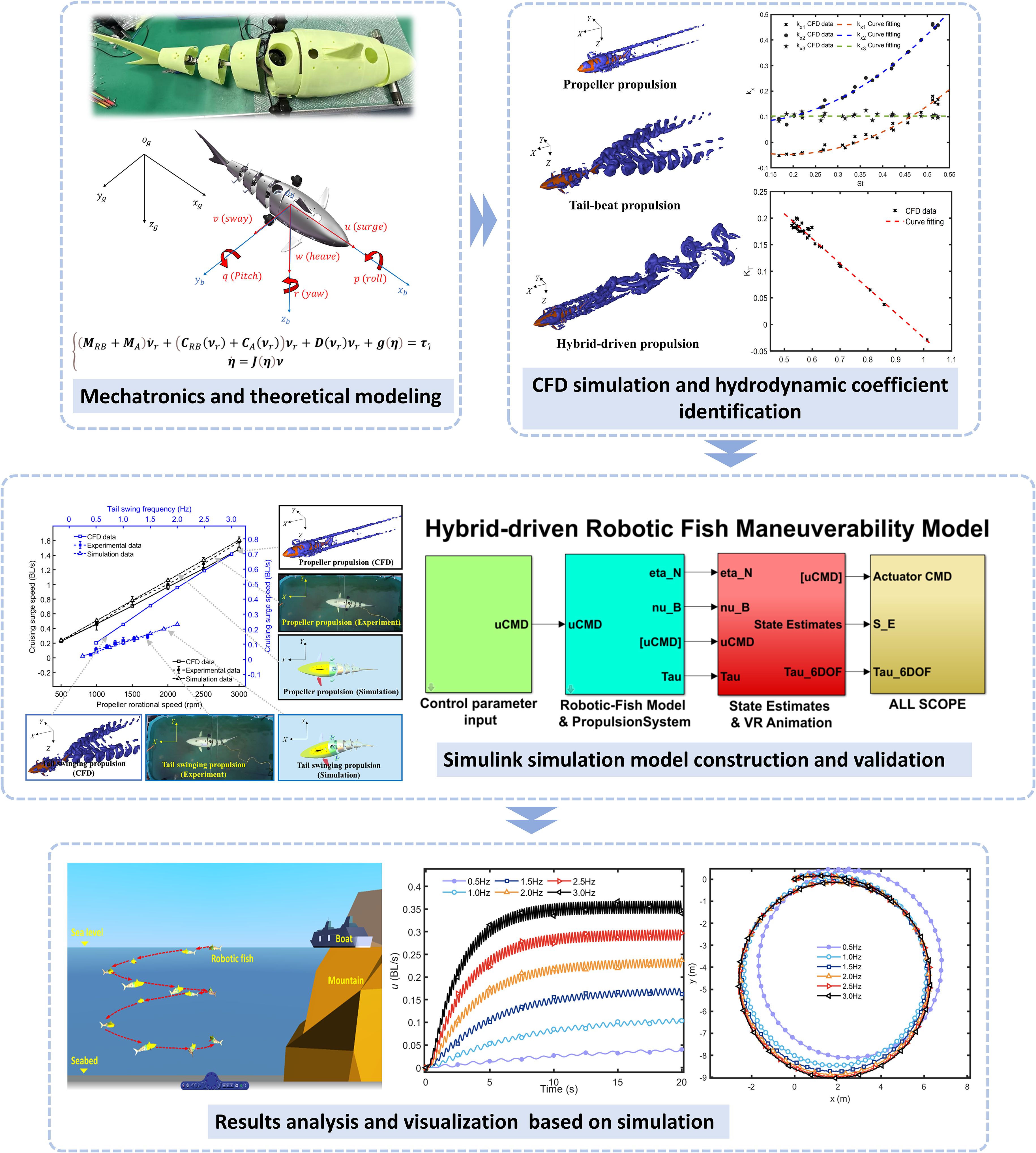
Figure 1. The framework of the overall research approach.

2 Mechatronics design of robotic fish

2.1 Mechanical structure

The designed and developed robotic fish is based on the biomimicry of a shark, as shown in Figure 2. It has a total length L of approximately 1.483 m, a body width W of about 0.45 m, the outermost distance of the pectoral fins is about 0.75 m, a body height H of about 0.45 m, and a total weight of approximately 48 kg. For detailed parameter information, please refer to Appendix A. The head contains the underwater camera, motion controller, power supply, and related onboard sensors of the robotic fish. The pectoral fins driven by four servomotors (RM-SV-40 underwater servomotors), the tail driven by three servomotors, and three propeller thrusters (T200-type thruster) provide the driving thrust for the robotic fish. Therefore, the robotic fish possesses both fish-inspired actuators-driving fins-and propeller thrusters commonly used in traditional underwater vehicles, offering three swimming modes: biomimetic driving, propeller driving, and hybrid driving. Thanks to the advantages of biomimetic swinging and propeller driving, the propulsion system of the robotic fish can provide stable thrust during long-distance and fast movement, and also achieve more precise and flexible maneuvering control when approaching the working area.

Figure 2

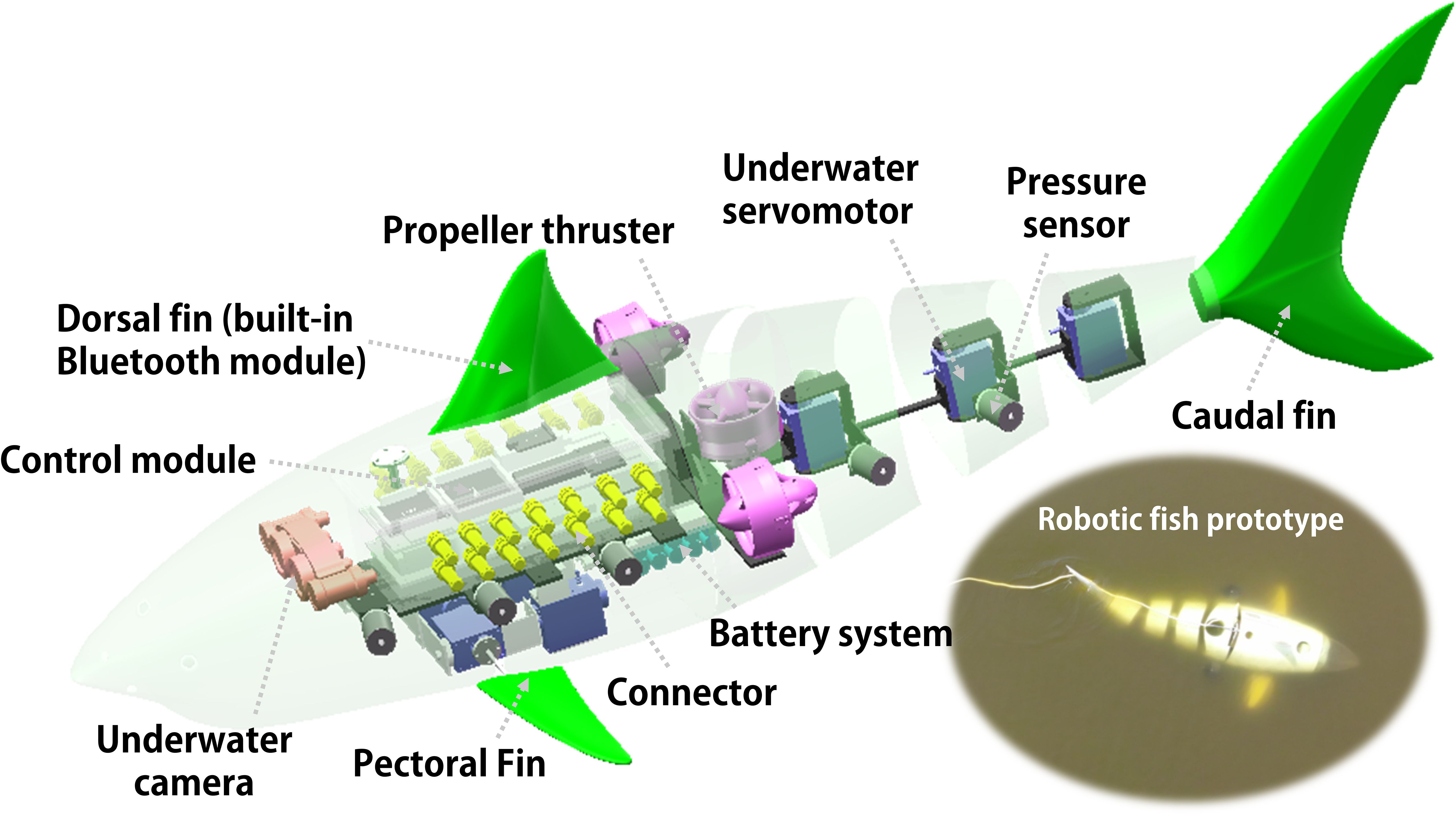
Figure 2. The design model and prototype of hybrid-driven robot fish.

It is also worth mentioning that in actual situations, when the horizontal propeller thrusters of the robotic fish rotate at the same speed, the thrust generated always extends along the body axis rather than the actual direction of movement. Due to the yaw motion of the body caused by the swinging of the tail, the robotic fish may not maintain good straight-line performance when both the tail swinging and the two horizontal propeller thrusters provide straight-line thrust. However, the combination of different actuators can effectively avoid this issue.

2.2 Working principle

The robotic fish also integrates an underwater camera, lateral line pressure sensors, and attitude sensors, capable of collecting pressure and attitude data from the sensors in real-time. It also has abundant sensor interfaces, allowing for flexible integration of various peripheral instruments. The working principle of the robotic fish is illustrated in Figure 3. Initially, the operator configures parameters via the upper-level computer software, including adjustments for underwater illumination and settings for control commands of the actuators (servomotors and propellers). Subsequently, the actuators commence operation, facilitating the movement of the robotic fish, including maneuvers such as forward motion, turning, ascending, and descending. Concurrently, the image and pressure sensors capture image and pressure information, respectively, generating data related to the robotic fish’s joint angles, environmental pressure, and temperature. These data are then transmitted back to the upper-level computer software for display and processing. The developed robotic fish prototype platform enables comprehensive control and monitoring of the robotic fish, providing a foundational basis for validating modeling and simulation theories as well as for subsequent control algorithm research.

Figure 3

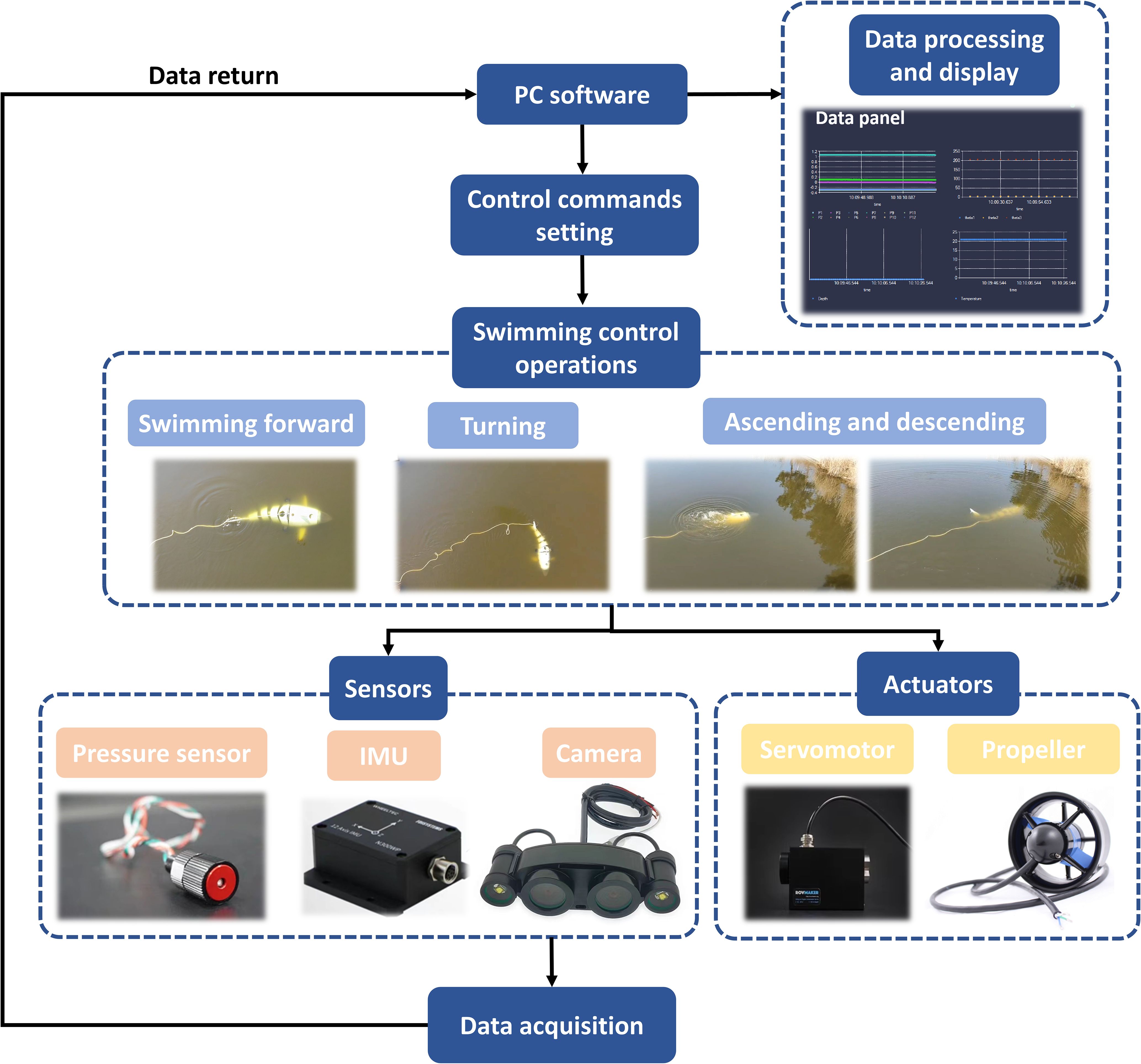
Figure 3. Working principle diagram.

3 Modeling of robotic fish

3.1 Kinematics

Define the earth-fixed reference frame $o_e{x}_e{y}_e{z}_e$ as the $\left\{e\right\}$ frame, the body-fixed reference frame $o_b{x}_b{y}_b{z}_b$ as the $\left\{b\right\}$ frame, and the origin of the $\left\{b\right\}$ frame is chosen to coincide with the center of gravity (CG) of the robotic fish. Therefore, the linear and angular velocity vector of the robot fish is described as $\dot{\eta }$ in th $\left\{e\right\}$e frame and v$\mathit{v}$ in the $\left\{b\right\}$ frame. The transformation between them is established as (Fossen, 1994) (Equation 1)

$\begin{array}{ll}\left[\begin{array}{c}{\dot{\mathit{\eta }}}_1\\ {\dot{\mathit{\eta }}}_2\end{array}\right]=\underset{J(\eta )}{\underbrace{\left[\begin{array}{cc}{\mathit{J}}_1({\mathit{\eta }}_2)& {\mathbf{0}}_{3\times 3}\\ {\mathbf{0}}_{3\times 3}& {\mathit{J}}_2({\mathit{\eta }}_2)\end{array}\right]}}\left[\begin{array}{c}{\mathit{\nu }}_1\\ {\mathit{\nu }}_2\end{array}\right]\iff \dot{\mathit{\eta }}=\mathit{J}(\mathit{\eta })\mathit{\nu }& (1)\end{array}$

Where, $\mathit{\eta }={[{\mathit{\eta }}_1^T,{\mathit{\eta }}_2^T]}^T$; ${\mathit{\eta }}_1={[x,y,z]}^T$; ${\mathit{\eta }}_2={[\varphi ,\theta ,\psi ]}^T$; $\mathit{\nu }={[{\mathit{\nu }}_1^T,{\mathit{\nu }}_2^T]}^T$; ${\mathit{\nu }}_1={[u,v,w]}^T$; ${\mathit{\nu }}_2={[p,q,r]}^T$. $\mathit{J}(\mathit{\eta })$ is a transformation matrix related through the Euler angles: roll ($\varphi$), pitch ($\theta$), yaw ($\psi$) according to Equations 2, 3

$\begin{array}{ll}{\mathit{\text{J}}}_{\mathbf{1}}({\mathit{\text{η}}}_{\mathbf{2}})=\left[\begin{array}{ccc}\cos \theta \cos \psi & \sin \varphi \sin \theta \cos \psi -\cos \varphi \sin \psi & \cos \varphi \sin \theta \cos \psi +\sin \varphi \sin \psi \\ \cos \theta \sin \psi & \sin \varphi \sin \theta \sin \psi +\cos \varphi \cos \psi & \cos \varphi \sin \theta \sin \psi -\sin \varphi \cos \psi \\ -\sin \theta & \sin \varphi \cos \theta & \cos \varphi \cos \theta \end{array}\right]& (2)\end{array}$

$\begin{array}{ll}{\mathit{J}}_2({\mathit{\eta }}_2)=\left[\begin{array}{ccc}1& \sin \varphi \tan \theta & \cos \varphi \tan \theta \\ 0& \cos \varphi & -\sin \varphi \\ 0& \sin \varphi /\cos \theta & \cos \varphi /\cos \theta \end{array}\right]& (3)\end{array}$

3.2 Six DOF rigid-body equations of motion

Based on Lagrangian Formulation, the robot fish’s six DOF rigid-body equations of motion can be expressed as Equation 4

$\begin{array}{ll}{\mathit{\text{M}}}_{\mathit{\text{RB}}}\dot{\mathit{\text{ν}}}+{\mathit{\text{C}}}_{RB}(\mathit{\text{ν}})\mathit{\text{ν}}={\mathit{\text{τ}}}_{RB}& (4)\end{array}$

Where, ${\mathit{\text{τ}}}_{RB}$ is a generalized vector of external forces and moments, ${\mathit{\text{M}}}_{RB}$ and ${\mathit{\text{C}}}_{RB}(\mathit{\text{ν}})$ are respectively the inertia matrix and Coriolis and centripetal matrix as Equations 5, 6

$\begin{array}{ll}{\mathit{\text{M}}}_{RB}=\left[\begin{array}{cc}m{\mathit{\text{E}}}_{3\times 3}& -m\mathit{\text{S}}({\mathit{\text{r}}}_G)\\ m\mathit{\text{S}}({\mathit{\text{r}}}_G)& {\mathit{\text{I}}}_0\end{array}\right]& (5)\end{array}$

$\begin{array}{ll}{\mathit{\text{C}}}_{RB}(\mathit{\text{ν}})=\left[\begin{array}{cc}{\mathbf{0}}_{3\times 3}& -m\mathit{\text{S}}({\mathit{\text{ν}}}_1)-m\mathit{\text{S}}({\mathit{\text{ν}}}_2)\mathit{\text{S}}({\mathit{\text{r}}}_G)\\ -m\mathit{\text{S}}({\mathit{\text{ν}}}_1)+m\mathit{\text{S}}({\mathit{\text{r}}}_G)\mathit{\text{S}}({\mathit{\text{ν}}}_2)& -\mathit{\text{S}}({\mathit{\text{I}}}_{\mathbf{0}}{\mathit{\text{ν}}}_2)\end{array}\right]& (6)\end{array}$

Where, $m$ is the mass of robotic fish, ${\mathit{\text{I}}}_0$ is the inertia tensor referred to the origin $o_b$, ${\mathit{\text{E}}}_{3\times 3}$ is the 3×3 identity matrix and $S(\lambda )$ is a skew-symmetrical matrix defined such that $\mathit{\text{λ}}\times \mathit{\text{a}}\triangleq \mathit{\text{S}}(\mathit{\text{λ}})\mathit{\text{a}}$, ${\mathit{\text{r}}}_G={[x_G,y_G,z_G]}^T$ is the vector from the origin $o_b$ to the robot fish's CG. Meanwhile, define ${\mathit{\text{r}}}_B={[x_B,y_B,z_B]}^T$ as the vector from origin $o_b$ to the robot fish's center of buoyancy (CB).

3.3 External forces and moments

The external forces and moments ${\mathit{\text{τ}}}_{RB}$ acting on the robotic fish’s CG during its motion in underwater space mainly consist of radiation-induced forces ${\mathit{\text{τ}}}_H$, environmental disturbance forces and moments ${\mathit{\text{τ}}}_E$ caused by underwater currents, as well as the control forces and moments ${\tau }_T$ generated by the actuators, that is Equation 7

$\begin{array}{ll}{\mathit{\text{τ}}}_{RB}={\mathit{\text{τ}}}_H+{\mathit{\text{τ}}}_E+{\mathit{\text{τ}}}_T& (7)\end{array}$

3.3.1 Radiation-induced forces

Radiation-induced forces can be categorized into three components: added mass forces and moments, hydrodynamic damping, and restoring forces and moments (Equation 8).

$\begin{array}{ll}{\mathit{\text{τ}}}_H=\underset{\begin{array}{l}\text{Added Mass}\\ \text{forces and moments} \end{array}}{\underbrace{-{\mathit{\text{M}}}_A\dot{\mathit{\text{ν}}}-{\mathit{\text{C}}}_{\mathit{\text{A}}}(\mathit{\text{ν}})\mathit{\text{ν}}}}-\underset{\begin{array}{l}\text{Hydrodynamic}\\ \text{damping} \end{array}}{\underbrace{\mathit{\text{D}}(\mathit{\text{ν}})\mathit{\text{ν}}}}-\underset{\begin{array}{l}\text{Restoring forces }\\ \text{and moments}\end{array}}{\underbrace{\mathit{\text{g}}(\mathit{\text{η}})}}& (8)\end{array}$

The added mass forces and moments are ${\mathit{\text{τ}}}_A=-{\mathit{\text{M}}}_A\dot{\mathit{\text{ν}}}-{\mathit{\text{C}}}_A(\mathit{\text{ν}})\mathit{\text{ν}}$, and the shape of the robot fish is approximately a regular geometry, then ${\mathit{\text{M}}}_A$ and ${\mathit{\text{C}}}_A(\mathit{\text{v}})$ are approximately expressed as Equations 9, 10

$\begin{array}{ll}{\mathit{\text{M}}}_A=\left[\begin{array}{cc}{\mathit{\text{M}}}_{11}& {\mathit{\text{M}}}_{12}\\ {\mathit{\text{M}}}_{21}& {\mathit{\text{M}}}_{22}\end{array}\right]=-\text{diag}\left\{X_{\dot{u}},Y_{\dot{v}},Z_{\dot{w}},K_{\dot{p}},M_{\dot{q}},N_{\dot{r}}\right\}& (9)\end{array}$

$\begin{array}{ll}{\mathit{\text{C}}}_A(\mathit{\text{ν}})=\left[\begin{array}{cc}{\mathbf{0}}_{3\times 3}& -\mathit{\text{S}}({\mathit{\text{M}}}_{11}{\nu }_1+{\mathit{\text{M}}}_{12}{\mathit{\text{ν}}}_2)\\ -\mathit{\text{S}}({\mathit{\text{M}}}_{11}{\mathit{\text{ν}}}_1+{\mathit{\text{M}}}_{12}{\mathit{\text{ν}}}_2)& -\mathit{\text{S}}({\mathit{\text{M}}}_{21}{\mathit{\text{ν}}}_1+{\mathit{\text{M}}}_{22}{\mathit{\text{ν}}}_2)\end{array}\right]& (10)\end{array}$

Where, the coefficients such as $X_{\dot{u}}$, $Y_{\dot{v}}$, and so on are added mass coefficients.

The hydrodynamic damping coefficient matrix that needs to be identified can be expressed as Equation 11

$\begin{array}{ll}\begin{array}{l}\mathit{\text{D}}(\mathit{\text{ν}})=-\text{diag}\left\{X_u,Y_v,Z_w,K_p,M_q,N_r\right\}\\ -\text{diag}\left\{X_{u\left|u\right|}\left|u\right|,Y_{v\left|v\right|}\left|v\right|,Z_{w\left|w\right|}\left|w\right|,K_{p\left|p\right|}\left|p\right|,M_{q\left|q\right|}\left|q\right|,N_{r\left|r\right|}\left|r\right|\right\}\end{array}& (11)\end{array}$

Where, the coefficients such as $X_u$, $Y_v$, and so on are linear damping coefficients. And the coefficients such as $X_{u\left|u\right|}$, $Y_{v\left|v\right|}$, and so on are quadratic damping coefficients.

The gravity and the buoyancy act on the CG and CB of the robot fish respectively, and the restoring force is expressed as Equation 12

$\begin{array}{ll}\mathit{\text{g}}(\mathit{\text{η}})=-\left[\begin{array}{c}{\mathit{\text{f}}}_G(\mathit{\text{η}})+{\mathit{\text{f}}}_B(\mathit{\text{η}})\\ \mathit{\text{S}}({\mathit{\text{r}}}_G){\mathit{\text{f}}}_G(\mathit{\text{η}})+\mathit{\text{S}}({\mathit{\text{r}}}_B){\mathit{\text{f}}}_B(\mathit{\text{η}})\end{array}\right]& (12)\end{array}$

Here, ${\mathit{\text{f}}}_G(\mathit{\text{η}})={\mathit{\text{J}}}_1^{-1}({\mathit{\text{η}}}_2)W{\mathit{\text{e}}}_3$, ${\mathit{\text{f}}}_B(\mathit{\text{η}})=-{\mathit{\text{J}}}_1^{-1}({\mathit{\text{η}}}_2)B{\mathit{\text{e}}}_3$, and they are the gravity and buoyancy in the $\left\{b\right\}$ frame, respectively.

3.3.2 Underwater current disturbances

The impact of underwater current disturbances ${\mathit{\text{τ}}}_E$ is incorporated into the robotic fish’s dynamics model by introducing the concept of relative velocity vector. Let the linear velocity vector of the current in the $\left\{e\right\}$ frame and the $\left\{b\right\}$ frame be denoted as ${\mathit{\text{ν}}}_s$ and ${\mathit{\text{ν}}}_c$, respectively. The conversion relationship between these vectors is given by ${\mathit{\text{ν}}}_c={\mathit{\text{J}}}_1^{-1}({\mathit{\text{η}}}_2){\mathit{\text{ν}}}_s$. Consequently, the linear velocity vector at which the robotic fish moves relative to the current in the $\left\{b\right\}$ frame can be expressed as ${\mathit{\text{ν}}}_1^r={\mathit{\text{ν}}}_1-{\mathit{\text{ν}}}_c$. By substituting ${\mathit{\text{ν}}}_1^r$ for ${\mathit{\text{ν}}}_1$, a new generalized velocity vector ${\mathit{\text{ν}}}_r({\dot{\mathit{\text{ν}}}}_r=\dot{\mathit{\text{ν}}}$) is obtained.

3.3.3 Control forces and moments

Hybrid-driven robotic fish utilize propeller thrusters, pectoral fins, and the three-joint tail as actuators to facilitate propulsion, as shown in Figure 4. Depending on the motion contributions of these actuators during horizontal and vertical maneuvers of the robotic fish, they are classified into two categories: horizontal actuators and vertical actuators, each assigned a unique identifier. The control forces and moments produced by these distinct actuators can be expressed as Equation 13

Figure 4

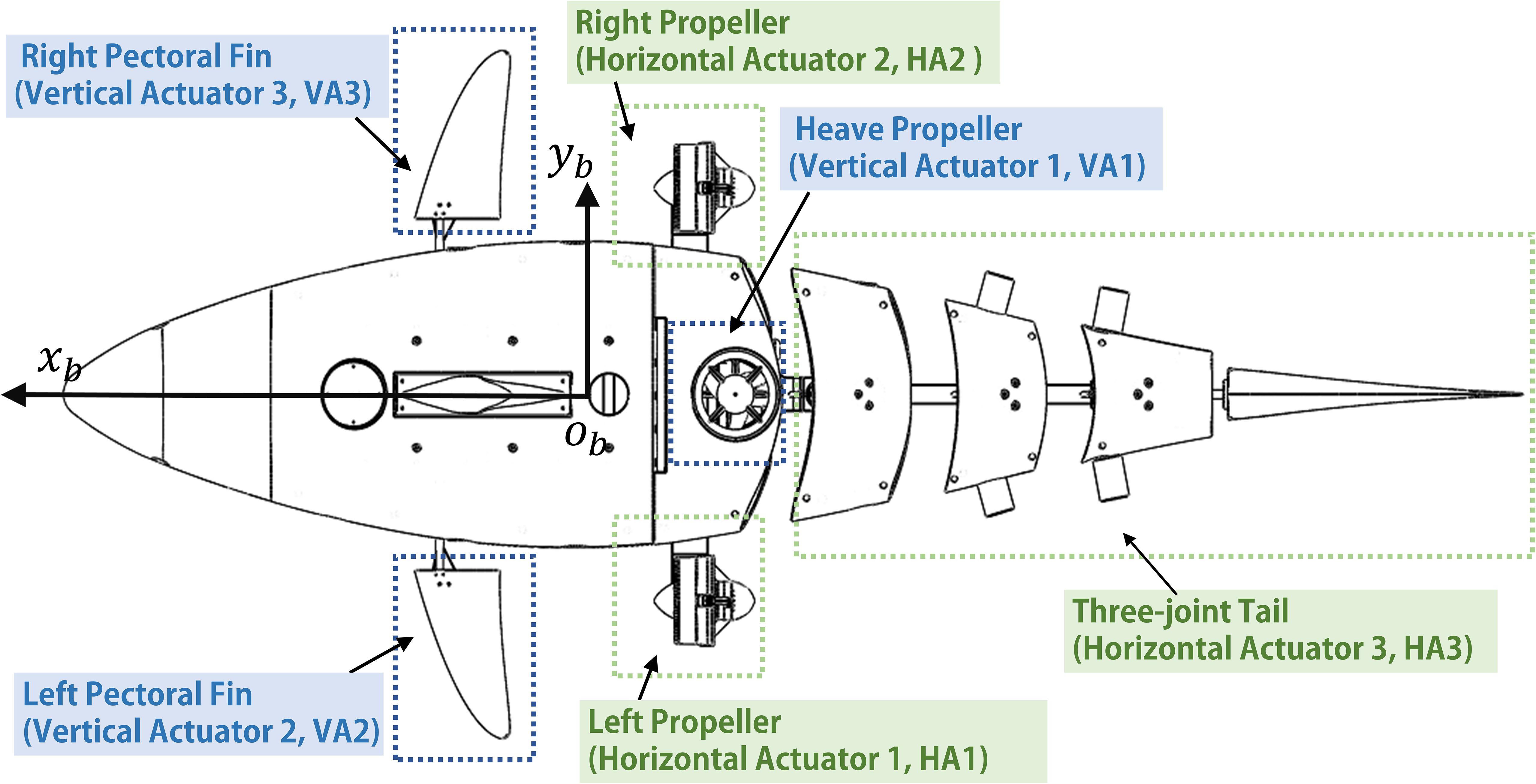
Figure 4. Horizontal and vertical actuators of hybrid-driven robotic fish.

$\begin{array}{ll}{\mathit{\text{τ}}}_T={\mathit{\text{τ}}}_{HA1\&HA2}+{\mathit{\text{τ}}}_{VA1}+{\mathit{\text{τ}}}_{VA2\&VA3}+{\mathit{\text{τ}}}_{HA3}& (13)\end{array}$

Where, ${\mathit{\text{τ}}}_{HA1HA2}$ and ${\mathit{\text{τ}}}_{VA2VA3}$ are respectively the resultant forces and moments generated by the left and right propellers and pectoral fins, ${\mathit{\text{τ}}}_{VA1}$ and ${\mathit{\text{τ}}}_{HA3}$ are respectively the forces and moments generated by the vertical propeller and three-joint tail.

3.3.3.1 Propeller thruster

The propeller thrust $T$ and moment $Q$ can be obtained by CFD simulation, then, the coefficients $K_T$ and $K_Q$ can be obtained as Equation 14

$\begin{array}{ll}\{\begin{array}{c}{K}_T=\frac{T}{\rho D^{4}n\left|n\right|}\\ K_Q=\frac{Q}{\rho D^{5}n\left|n\right|}\end{array}& (14)\end{array}$

Where, $\rho$ is the fluid density, $n$ is the rotational speed of the propeller, and $D$ is the diameter of the propeller. Moreover, the relationship between the advance number $J$ and these coefficients was established.

The force and moment generated by the HA2 actuator of the robot fish is shown as Figure 5a. The force generated by the HA2 actuator is $T_{\text{HA}2}{\mathit{\text{e}}}_1$, and the moment is $Q_{\text{HA}2}{\mathit{\text{e}}}_1+\mathit{\text{S}}({\mathit{\text{r}}}_{\text{HA}2})T_{\text{HA}2}{\mathit{\text{e}}}_1$. Where, ${\mathit{\text{r}}}_{\text{HA}2}$ is the vector from $o_b$ to the force center of HA2, and $\mathit{\text{S}}({\mathit{\text{r}}}_{\text{HA}2})T_{\text{HA}2}{\mathit{\text{e}}}_1$ is the moment generated by $T_{\text{HA}2}{\mathit{\text{e}}}_1$ relative to the $\left\{b\right\}$ frame. We can ignore $Q_{\text{HA}2}{\mathit{\text{e}}}_1$ because of $\Vert Q_{\text{HA}2}{\mathit{\text{e}}}_1\Vert \ll \Vert \mathit{\text{S}}({\mathit{\text{r}}}_{\text{HA}2})T_{\text{HA}2}{\mathit{\text{e}}}_1\Vert$, so that the resultant force and moment generated by the HA1 and HA2 actuators can be expressed as Equation 15

Figure 5

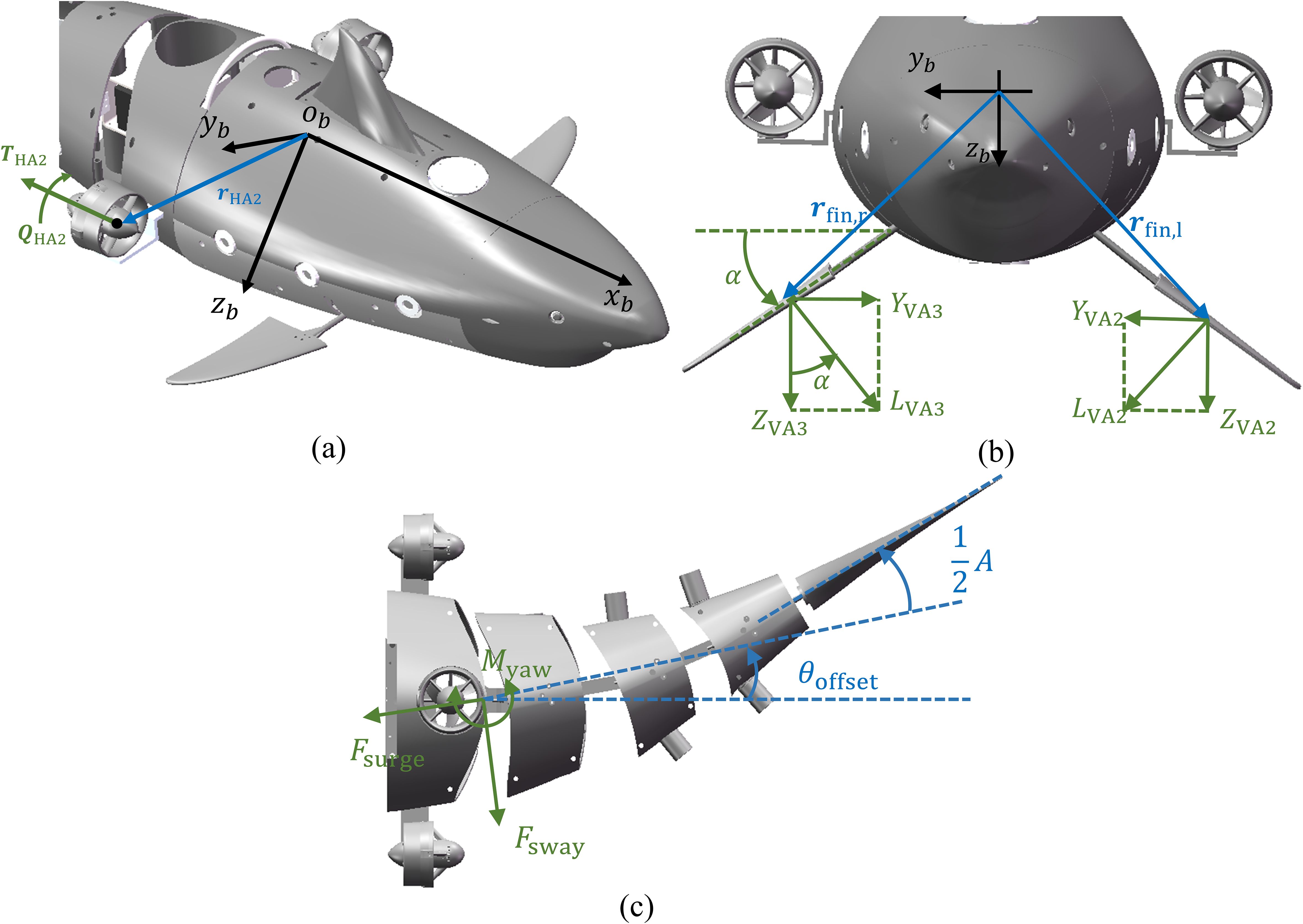
Figure 5. Control force analysis of robot fish’s motion actuators. (a) The HA2 actuator; (b) The VA2 and VA3 actuators; (c) The HA3 actuator.

$\begin{array}{ll}\begin{array}{l}{\mathit{\text{τ}}}_{\text{HA}1\text{HA}2}=\left[\begin{array}{c}(T_{\text{HA}1}+T_{\text{HA}2}){\mathit{\text{e}}}_1\\ \mathit{\text{S}}({\mathit{\text{r}}}_{\text{HA}1})T_{\text{HA}1}{\mathit{\text{e}}}_1+\mathit{\text{S}}({\mathit{\text{r}}}_{\text{HA}2})T_{\text{HA}2}{\mathit{\text{e}}}_1\end{array}\right]\\ =\rho D^4{K}_T\left[\begin{array}{cc}{e}_1& e_1\\ \mathit{\text{S}}({\mathit{\text{r}}}_{\text{HA}1}){\mathit{\text{e}}}_1& \mathit{\text{S}}({\mathit{\text{r}}}_{\text{HA}2}){\mathit{\text{e}}}_1\end{array}\right]\left[\begin{array}{c}{n}_{\text{HA}1}\left|n_{\text{HA}1}\right|\\ n_{\text{HA}2}\left|n_{\text{HA}2}\right|\end{array}\right]\end{array}& (15)\end{array}$

Where, $n_{\text{HA}1}$ and $n_{\text{HA}2}$ are respectively the rotational speed of the HA1 and HA2 actuators, and $e_1$ is a unit vector pointing in the positive direction of the $o_b{x}_b$ axis.

Similarly, the force and moment provided by the VA1 actuator can be expressed as Equation 16

$\begin{array}{ll}{\mathit{\text{τ}}}_{\text{VA}1}=\left[\begin{array}{c}{T}_{\text{VA}1}{\mathit{\text{e}}}_3\\ \mathit{\text{S}}({\mathit{\text{r}}}_{\text{VA}1})T_{\text{VA}1}{\mathit{\text{e}}}_3\end{array}\right]=\rho D^4{K}_T{n}_{\text{VA}1}\left|n_{\text{VA}1}\right|\left[\begin{array}{c}{\mathit{\text{e}}}_3\\ \mathit{\text{S}}({\mathit{\text{r}}}_{\text{VA}1}){\mathit{\text{e}}}_3\end{array}\right]& (16)\end{array}$

Where, ${\mathit{\text{r}}}_{\text{VA}1}$ is the vector from $o_b$ to the force action center of VA1, $n_{\text{VA}1}$ is the rotational speed of the VA1 actuator and ${\mathit{\text{e}}}_3$ is a unit vector pointing in the positive direction of the $o_b{z}_b$ axis.

3.3.3.2 Pectoral fin

The hybrid-driven robotic fish we developed features two pectoral fins (the VA2 and VA3 actuators) that influence its heave motion, pitch angle, and roll angle, with each fin possessing two DOF. As shown in Figure 5b, the motion and force analysis of them is conducted using the VA3 actuator as an example. The flapping angle is defined as $\alpha$, and the rotating angle as $\delta$. If the flapping angles $\alpha$ of the VA2 and VA3 actuators are equal, then for a fixed $\alpha$, the position vectors from $o_b$ to the force centers of the VA2 and VA3 actuators are given by ${\mathit{\text{r}}}_{\text{fin},\text{r}}={[x_{\text{fin}},y_{\text{fin}},z_{\text{fin}}]}^T$, ${\mathit{\text{r}}}_{\text{fin},\text{l}}={[x_{\text{fin}},-y_{\text{fin}},z_{\text{fin}}]}^T$, respectively. The rotating angles of the VA2 and VA3 actuators relative to the body are denoted as ${\delta }_{\text{VA}2}$ and ${\delta }_{\text{VA}3}$. Using the empirical formula for lift experienced by the airfoil, the lift generated by VA2 and VA3 actuators can be expressed as Equation 17

$\begin{array}{ll}{L}_{\text{VA}2\&\text{VA}3}=\frac{1}{2}\rho c_L{S}_{\text{fin}}(u^2{\delta }_{\text{VA}2\&\text{VA}3}+uw-x_{\text{fin}}uq)& (17)\end{array}$

As shown in Figure 5b, through the flapping angle $\alpha$, $L_{\text{VA}2}$ and $L_{\text{VA}3}$ can be decomposed into the following forces and moments in the $\left\{b\right\}$ frame (Equation 18).

$\begin{array}{ll}\begin{array}{cc}\{\begin{array}{l}{Y}_{\text{VA}2}=L_{\text{VA}2}\sin \alpha \hfill \\ Z_{\text{VA}2}=L_{\text{VA}2}\cos \alpha \hfill \\ K_{\text{VA}2}=-y_{\text{fin}}{Z}_{\text{VA}2}-z_{\text{fin}}{Y}_{\text{VA}2}\hfill \\ M_{\text{VA}2}=-x_{\text{fin}}{Z}_{\text{VA}2}\hfill \\ N_{\text{VA}2}=x_{\text{fin}}{Y}_{\text{VA}2}\hfill \end{array}& \{\begin{array}{l}{Y}_{\text{VA}3}=-L_{\text{VA}3}\text{sin}\alpha \hfill \\ Z_{\text{VA}3}=L_{\text{VA}3}\text{cos}\alpha \hfill \\ K_{\text{VA}3}=y_{\text{fin}}{Z}_{\text{VA}3}-z_{\text{fin}}{Y}_{\text{VA}3}\hfill \\ M_{\text{VA}3}=-x_{\text{fin}}{Z}_{\text{VA}3}\hfill \\ N_{\text{VA}3}=x_{\text{fin}}{Y}_{\text{VA}3}\hfill \end{array}\end{array}& (18)\end{array}$

Therefore, the resultant force and moment generated by the VA2 and VA3 actuators can be expressed as Equation 19

$\begin{array}{ll}{\mathit{\text{τ}}}_{\text{VA}2\&\text{VA}3}=\left[\begin{array}{c}0\\ Y_{\text{VA}2}+Y_{\text{VA}3}\\ Z_{\text{VA}2}+Z_{\text{VA}3}\\ K_{\text{VA}2}+K_{\text{VA}3}\\ M_{\text{VA}2}+M_{\text{VA}3}\\ N_{\text{VA}2}+N_{\text{VA}3}\end{array}\right]& (19)\end{array}$

3.3.3.3 Three-joint tail

Define the rotation angle of the i-th (where i = 1, 2, 3) motion joint of the robotic fish as ${\theta }_i$ rad. In this study, we fix the robotic fish’s tail swing amplitude A to be approximately 0.12 times the body length (BL). Based on the joint length conditions, the three-joint tail moving at a tail swing frequency $f$ has its swinging pattern fitted using an exponential fish-like body wave (Xue et al., 2020), specifically as Equation 20

$\begin{array}{ll}\{\begin{array}{c}{\theta }_1=0.0973\sin (2\text{π}ft+1.635)\left(1-{\text{e}}^{-\frac{t}{0.2}}\right)\\ {\theta }_2=0.0760\sin (2\text{π}ft+2.031)\left(1-{\text{e}}^{-\frac{t}{0.2}}\right)\\ {\theta }_3=0.134\sin (2\text{π}ft+2.356)\left(1-{\text{e}}^{-\frac{t}{0.2}}\right)\end{array}& (20)\end{array}$

The Strouhal number St is a dimensionless parameter used to characterize oscillatory flow phenomena and can be employed to describe the propulsion movement of fish (Triantafyllou, 1993). It directly governs the formation pattern and shedding frequency of the wake vortex street, thereby serving as the key dimensionless criterion in wake-vortex modeling for matching vortex strength with thrust pulsations. And it is defined as $\text{St}=\frac{fA}{U_s}$, where $U_s=\Vert {\nu }_1{\Vert }_2$, represents the steady-state cruising speed. Using CFD software for numerical analysis and simulation of the robotic fish’s movement, previous numerical studies (Costa et al., 2020; Yu and Huang, 2021) have indicated that: under the condition of a fixed tail swing amplitude A, the hydrodynamic coefficient of the actuator HA3 (with the force center at the intersection of the first tail joint’s rotation axis and the $o_b{x}_b{y}_b$ plane) is a function of the Strouhal number St and the tail swing frequency $f$. Therefore, the force and moment can be expressed as Equation 21

$\begin{array}{ll}\{\begin{array}{c}{F}_{\text{surge}}=\frac{1}{2}\rho U^2{S}_{\text{Tail}}{C}_T(\text{St,}f)\\ F_{\text{sway}}=\frac{1}{2}\rho U^2{S}_{\text{Tail}}{C}_L(\text{St,}f)\\ M_{\text{yaw}}=\frac{1}{2}\rho U^2{S}_{\text{Tail}}{C}_M(\text{St,}f)\end{array}& (21)\end{array}$

Where, $S_{\text{Tail}}$ represents the effective area during tail swinging, and $C_T(\text{St,}f)$, $C_L(\text{St,}f)$, and $C_M(\text{St,}f)$ are the surge thrust coefficient, sway force coefficient, and yaw moment coefficient of the robotic fish’s tail, respectively, obtained through CFD calculations.

The periodic asymmetric swinging of the robotic fish’s tail causes it to move in a curved path (turning motion). To account for this while simplifying the complexity of modeling the tail actuator HA3, a bias angle ${\theta }_{\text{offset}}$ is introduced only at the first joint of the tail. As shown in Figure 5c, after considering the bias angle ${\theta }_{\text{offset}}$ of the swing tail, the control force and moment generated by the tail actuator HA3 can be expressed as Equation 22

$\begin{array}{ll}\{\begin{array}{c}{\tau }_{\text{surge},\text{HA}3}=F_{\text{surge}}\cos {\theta }_{\text{offset}}-F_{\text{sway}}\sin {\theta }_{\text{offset}}\\ {\tau }_{\text{sway},\text{HA}3}=F_{\text{surge}}\sin {\theta }_{\text{offset}}+F_{\text{sway}}\cos {\theta }_{\text{offset}}\\ {\tau }_{\text{yaw},\text{HA}3}=M_{\text{yaw}}-l_{\text{d}}{\tau }_{\text{sway},\text{HA}3}\end{array}& (22)\end{array}$

Here, $l_{\text{d}}$ denotes the distance from the center of the tail force to $o_b$. That is, the force and moment generated by the tail actuator HA3 are Equation 23

$\begin{array}{ll}{\mathit{\text{τ}}}_{\text{HA}3}={[\begin{array}{cccccc}{\tau }_{\text{surge},\text{HA}3}& {\tau }_{\text{sway},\text{HA}3}& 0& 0& 0& {\tau }_{\text{yaw},\text{HA}3}\end{array}]}^{\text{T}}& (23)\end{array}$

3.4 Equation of motion

After thorough analysis, we have derived the final nonlinear equation of motion, which in the body-fixed frame can be written as Equation 24.

$\begin{array}{ll}\{\begin{array}{c}({\mathit{\text{M}}}_{RB}+{\mathit{\text{M}}}_A)\dot{\mathit{\text{v}}}+({\mathit{\text{C}}}_{RB}(\mathit{\text{v}})+{\mathit{\text{C}}}_A({\mathit{\text{v}}}_r)){\mathit{\text{v}}}_r+D({\mathit{\text{v}}}_r){\mathit{\text{v}}}_r+g(\mathit{\text{η}})={\mathit{\text{τ}}}_T\\ \dot{\mathit{\text{η}}}=\mathit{\text{J}}(\mathit{\text{η}})\mathit{\text{v}}\end{array}& (24)\end{array}$

4 Hydrodynamic coefficient identification

4.1 Added mass coefficients

Since the added mass coefficient is not affected by the oscillation frequency of the robotic fish, it can be assumed to be constant (Fossen, 1994). In the mathematical model, it is reasonable to assume that the shape of the robotic fish is an elongated ellipsoid. The formula for the diagonal added mass coefficient of the equivalent elongated ellipsoid (Ahmad Mazlan, 2015) is listed in Equation 25.

$\begin{array}{ll}\begin{array}{l}{X}_{\dot{u}}\hspace{0.17em}=-\frac{{\alpha }_0}{2-{\alpha }_0}m\\ Y_{\dot{v}}\hspace{0.17em}=Z_{\dot{w}}=-\frac{{\beta }_0}{2-{\beta }_0}m\\ K_{\dot{p}}\hspace{0.17em}=0\\ N_{\dot{r}}\hspace{0.17em}=M_{\dot{q}}=-\frac{1}{5}\frac{{(b^2-a^2)}^2({\alpha }_0-{\beta }_0)}{2(b^2-a^2)+(b^2+a^2)({\beta }_0-{\alpha }_0)}m\\ {\alpha }_0\hspace{0.17em}=\frac{2(1-e^2)}{e^3}\left(\frac{1}{2}\text{ln}\frac{1+e}{1-e}-e\right)\\ {\beta }_0\hspace{0.17em}=\frac{1}{e^2}-\frac{1-e^2}{2e^3}\text{ln}\frac{1+e}{1-e}\end{array}& (25)\end{array}$

Where, a, b, and c are the lengths of the three semi-axes of the robotic fish’s equivalent ellipsoid, $e=1-{(b/a)}^2$ is the eccentricity, ${\alpha }_0$ and ${\beta }_0$ are variables related to e. Based on the calculations of the equivalent ellipsoid dimensions of the robotic fish, the added mass coefficients of the robotic fish can be determined, as shown in Appendix A.

4.2 CFD numerical model

4.2.1 Computational domain construction

CFD simulations are employed to determine the hydrodynamic damping coefficients, thrust coefficients of swing tail, and thrust coefficients of propeller required for developing the mathematical model of the robotic fish. Initially, the propeller propulsion system and the three-joint tail propulsion system of the robotic fish are kept stationary relative to the head. The robotic fish is then subjected to various translational (sway, surge, heave) and rotational (roll, pitch, yaw) motions at different velocities, and the hydrodynamic damping coefficients are calculated for each direction individually. Subsequently, by simulating the self-propulsion of the robotic fish with different propeller rotational speeds and tail swing frequencies, and after determining the hydrodynamic conditions acting on the robotic fish, the thrust coefficients of the swing tail and the propeller are calculated. the robotic fish’s self-propulsion movement only considers planar translational motion and does not account for the head’s yaw oscillation. This is not an oversimplification or oversight but rather a necessary compromise for simulating the tail movement under different Strouhal numbers and acquiring thrust data from the three-joint tail and propeller propulsion system during the movement. To facilitate CFD simulations, the 3D model was simplified to a certain extent while retaining key geometric features, with virtual hinges between each joint.

A unified numerical simulation domain for a 3D virtual water tank flow field, with the dimensions of the virtual water tank set to: $8.5L\times 6.5W\times 7.5H$ are constructed. Overlapping grid technology is employed to enable the robotic fish to perform translational and rotational movements in various directions. A combination of dynamic and overlapping grids is used to simulate the swinging motion of the robotic fish’s three-joint tail relative to the $\left\{b\right\}$ frame, as well as the forward swimming of the robotic fish relative to the $\left\{e\right\}$ frame (Xue et al., 2023) [(substituting the movement of a small surrounding flow field around the robotic fish for itself]. Sliding grids are utilized to facilitate the rotational motion of the propeller thrusters relative to the $\left\{b\right\}$ frame.

As depicted in Figure 6A, both background and component grids are established, including the rotational domain of the propeller thrusters. Independent component grids are created for the outer flow field regions of the robotic fish tail’s three joints, which are nested within the component grids of the overall outer flow field region that encloses the entire robotic fish. The component grids of the overall region are also nested within the background grid. A velocity-inlet boundary condition is applied with 0 m/s, and a pressure-outlet boundary condition is set with 0 Pa. The exterior surfaces of the robotic fish are defined as no-slip walls. The overlapping regions are designated as overset surfaces, and the grid sliding regions are set as interfaces.

Figure 6

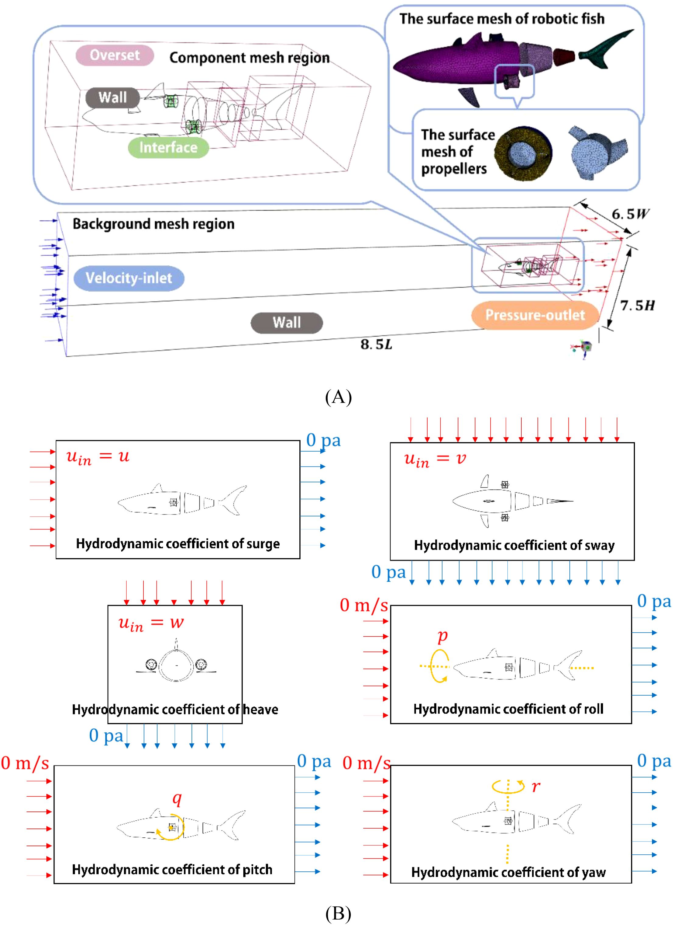
Figure 6. Computational domain and boundary condition settings. (A) Self-propulsion simulation setup for the robotic fish; (B) Six DOF hydrodynamic damping coefficients solution setup.

As shown in Figure 6B, for the robotic fish’s sway, surge, and heave motions, the relative motion between the robotic fish and the surrounding fluid domain is equivalently replaced by fixing the position of the robotic fish and varying the inlet velocity of the velocity-inlet boundary condition. The inlet velocity for the velocity-inlet boundary condition in different directions is set to $u_{in}$ m/s, with the pressure-outlet boundary condition set to 0 Pa, and all other boundary conditions remain consistent with the aforementioned setup. For the robotic fish’s roll, pitch, and yaw motions, the overlapping grid technique is employed to define the relative rotational motion of the robotic fish’s overlapping region. The inlet velocity for the velocity-inlet boundary condition is set to 0 m/s, with the pressure-outlet boundary condition set to 0 Pa, and all other boundary conditions remain consistent with the aforementioned setup.

The control equations for the numerical simulation domain of the hybrid-driven robotic fish are the averaged continuity equation and the Reynolds-averaged Navier-Stokes (RANS) equations in a 3D Cartesian coordinate system for incompressible flow (Versteeg and Malalasekera, 2007). To effectively solve these control equations, the following computational settings are chosen: a pressure-based solver, absolute velocity formulation, and transient time model; the k-ω SST turbulence model; the Coupled algorithm for pressure-velocity coupling; in the solution methods, the gradient calculation uses a least-squares cell-based approach, the pressure term uses a second-order discretization scheme, the momentum term uses a second-order upwind scheme, and both the turbulent kinetic energy and dissipation rate use a second-order upwind scheme. The transient calculation scheme is first-order implicit, and other solution control parameters are in their general form. Additionally, the motion state of the robotic fish and the net force ${\tau }_{\text{BodyNet}}$ acting on the robotic fish’s body, as well as the force ${\tau }_{\text{prop}}$ experienced by the propeller thrusters, are monitored.

4.2.2 Grid and time-step size independence verification

To enhance solution accuracy and conserve computational resources, a verification of grid size and time-step independence relative to simulation results is conducted to determine the most appropriate grid and time-step size. The background and component grid regions of the computational domain are divided into five size levels, with the requirement that the minimum orthogonal quality of all grids, except for the boundary layer, should not be less than 0.3. Five sets of body cell grid models are generated, corresponding to coarse, coarser, normal, finer, and fine levels (grid counts for different size levels: 390,974, 573,855, 947,726, 2,104,248, and 4,320,628). During the independence verification simulations using grids of different levels, the tail swing frequency and the propeller rotational speed are respectively set to 2 Hz and 1500 rpm, simulating the self-propulsion movement of the robotic fish under the hybrid-driven system. The surge cruising speed of the robotic fish after reaching a stable swimming state is designated as the observation parameter to verify independence.

As shown in Figure 7A, the cruising speed results for the normal grid level gradually converge with those of subsequent grids. Therefore, the normal-sized grid is selected for the time-step independence verification and subsequent formal simulation. Similarly, the time step is divided into five levels to verify its independence relative to the simulation results: 0.0025 s, 0.005 s, 0.0075 s, 0.001 s, and 0.00125 s. As depicted in Figure 7B, to ensure computational accuracy while minimizing the computational period and facilitating data storage, a time step of 0.01 s is chosen for the subsequent simulation process.

Figure 7

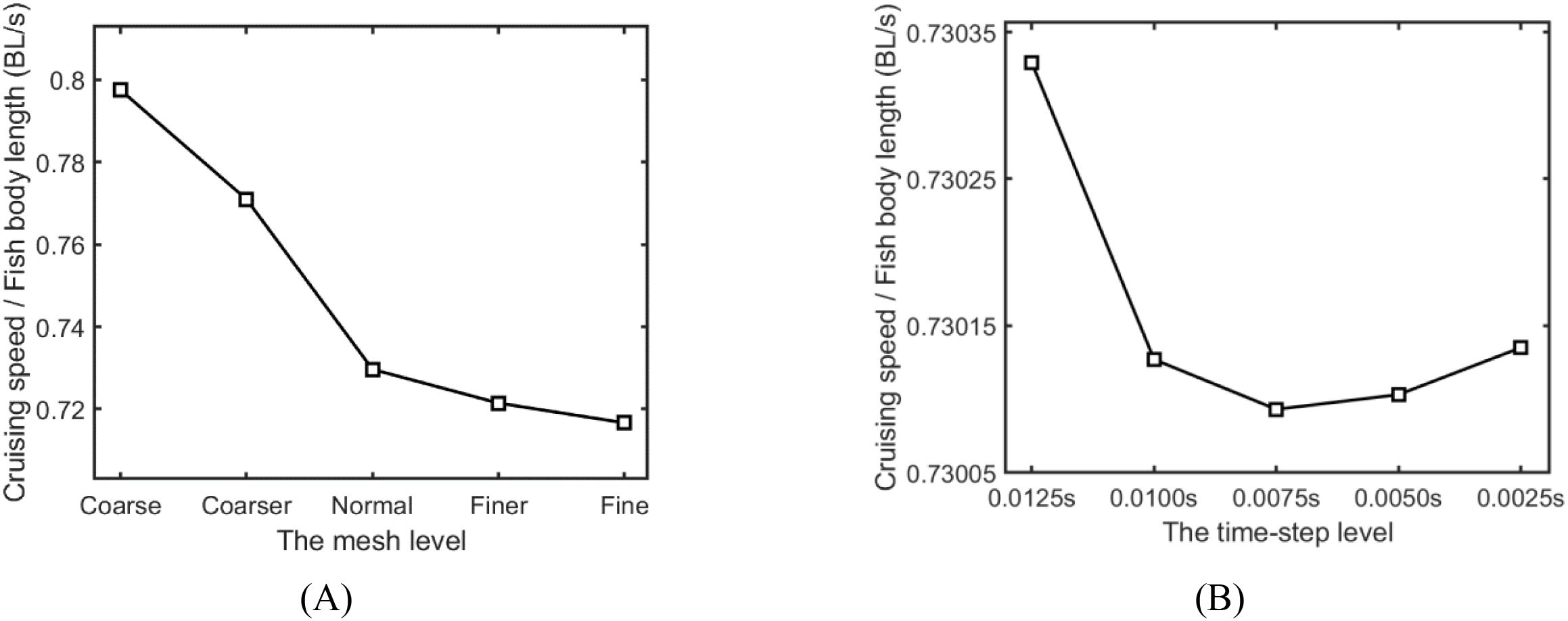
Figure 7. The results of independence verification. (A) Grid size. (B) Time-step size.

4.3 Damping coefficients identification

When the robotic fish moves in 3D space, the hydrodynamic damping forces it experiences in each direction are opposite to the corresponding velocity directions. When calculating the hydrodynamic coefficients for sway, surge, and heave, the velocity inlet $u_{in}$ is defined for each direction as $u=0\sim 2$ m/s, $v=0\sim 1$ m/s, and $w=0\sim 1$ m/s, respectively. For calculating the hydrodynamic coefficients of roll, pitch, and yaw, the rotational velocities of the robotic fish along the three directions are defined as $p=q=r=$ 0.1745~0.8757 rad/s (equivalent to 10~50°/s). Through CFD simulations, the converged values of the hydrodynamic damping forces and moments in the sway, surge, heave, roll, pitch, and yaw directions were obtained at different motion velocities. The CFD data and fitted curves that include standard deviation (std) bounds are shown in Figure 8. The coefficients of determination (R²) for all curves are close to 1, indicating excellent fits and allowing for the determination of the damping coefficients for sway, surge, heave, roll, pitch, and yaw of the robotic fish, as detailed in Appendix A.

Figure 8

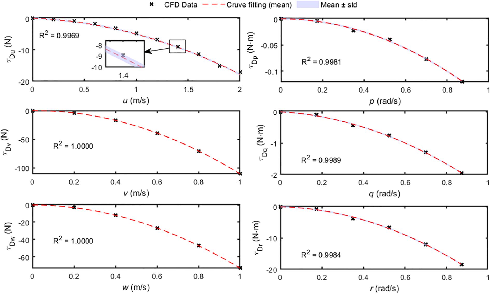
Figure 8. Hydrodynamic damping fitting.

4.4 Thrust coefficients of tail and propellers

4.4.1 Self-propulsion simulation parameter configuration

User-defined functions (UDF) are employed to define the tail swinging and propeller rotation of the robotic fish, simulating its transition from a stationary state to a converged state with stable forward swimming speed. By simulating the swimming motion of the robotic fish under various propeller rotational speeds and tail swing frequencies, the hydrodynamic coefficient variations of the tail and propellers in single or hybrid-driven modes are investigated. Eight propeller rotational speeds ranging from 500 rpm to 3000 rpm and six servomotor rotation frequencies ranging from 0.5 Hz to 3.0 Hz are set, resulting in 14 parameter configurations for single-driven mode. Combining these parameters, 24 parameter configurations for hybrid-driven mode are selected, with the detailed configuration methods shown in Table 1 (where “○” and “×” in the table indicate whether the condition is selected).

Table 1

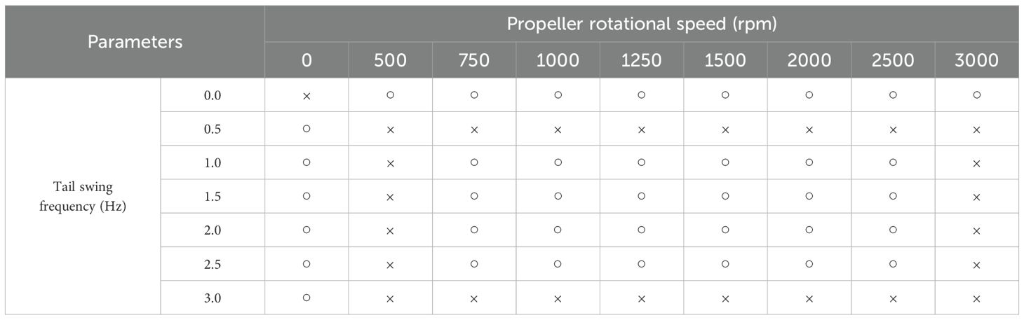
Table 1. Parameter configurations.

4.4.2 Thrust coefficients

4.4.2.1 Three-joint tail

In the process of the hybrid-driven robotic fish accelerating from rest to the cruising swimming speed, thrust is provided by the tail and propeller thrusters. Once the cruising swimming speed is reached (force equilibrium), the net force experienced by the fish’s body is counterbalanced by the force exerted by the propeller thrusters, i.e., ${\mathit{\text{τ}}}_{\text{BodyNet}}+{\mathit{\text{τ}}}_{\text{prop}}=0_{6\times 1}$. The thrust provided by the tail, ${\mathit{\text{τ}}}_{\text{HA}3}$, can be calculated as the sum of the net force on the fish’s body at cruising speed, ${\mathit{\text{τ}}}_{\text{BodyNet}}$, and the damping, ${\mathit{\text{τ}}}_{\text{D}}$ (where ${\mathit{\text{τ}}}_{\text{D}}$ is computed using the aforementioned hydrodynamic damping coefficients). Through CFD simulations, the forces and moments $F_{\text{surge}}$, $F_{\text{sway}}$, and $M_{\text{yaw}}$ acting on the fish’s tail can be obtained. Furthermore, the instantaneous variations of $C_T$, $C_L$, and $C_M$ can be determined using Equation 21. By employing curvilinear regression methods to fit the variation curves of these coefficients, the instantaneous variation patterns of the thrust coefficients of swing tail, represented by trigonometric functions, are obtained for different tail swing frequencies and propeller rotational speed configurations as Equation 26:

$\begin{array}{ll}\begin{array}{c}{C}_T=k_{\text{x}1}+k_{\text{x}2}\sin (4\pi ft+k_{\text{x}3})\\ C_L=k_{\text{y}1}\sin (2\pi ft+k_{\text{y}2})\\ C_M=k_{\text{z}1}\sin (2\pi ft+k_{\text{z}2})\end{array}& (26)\end{array}$

Where, $k_{\text{x}1}$, $k_{\text{x}2}$, $k_{\text{x}3}$, $k_{\text{y}1}$, $k_{\text{y}2}$, $k_{\text{z}1}$, $k_{\text{z}2}$ are the parameters related to the tail thrust coefficients, as detailed in Appendix B.

It is worth noting that the parameters $k_{\text{x}1}$, $k_{\text{x}2}$, and $k_{\text{x}3}$ can represent the mean value of the surge thrust coefficient $C_T$ over a certain period, the amplitude of periodic oscillation, and the phase, respectively, with similar interpretations for other parameters. By employing curvilinear regression analysis to examine the relationship between the hydrodynamic coefficient parameters and the Strouhal number St. It is found that $k_{\text{x}1}$, $k_{\text{x}2}$, $k_{\text{y}1}$, and $k_{\text{z}1}$ can be approximated as quadratic functions of St, while $k_{\text{x}3}$, $k_{\text{y}2}$, and $k_{\text{z}2}$ can be considered as constants, as shown in Figure 9. The results are as follows: $k_{\text{x}1}=0.01797-0.7047St+1.905S{t}^2$, $k_{\text{x}2}=0.09809-0.3937St+2.081S{t}^2$, $k_{\text{x}3}=0.1025$, $k_{\text{y}1}=20.97S{t}^2$, $k_{\text{y}2}=3.205$, $k_{\text{z}1}=17.16S{t}^2$, and $k_{\text{z}2}=13.31$. Consequently, the time-varying patterns of the thrust coefficients of swing tail $C_T$, $C_L$, and $C_M$ with respect to the Strouhal number St and tail swing frequency $f$ are obtained. It is observed that when $St<0.33$, $k_{\text{x}1}<0$, indicating that the robotic fish’s tail cannot provide effective positive thrust at this point. For a complementary perspective on how the Strouhal number influences the wake field of the robotic fish, we have provided relevant discussion in the Supplementary Material.

Figure 9

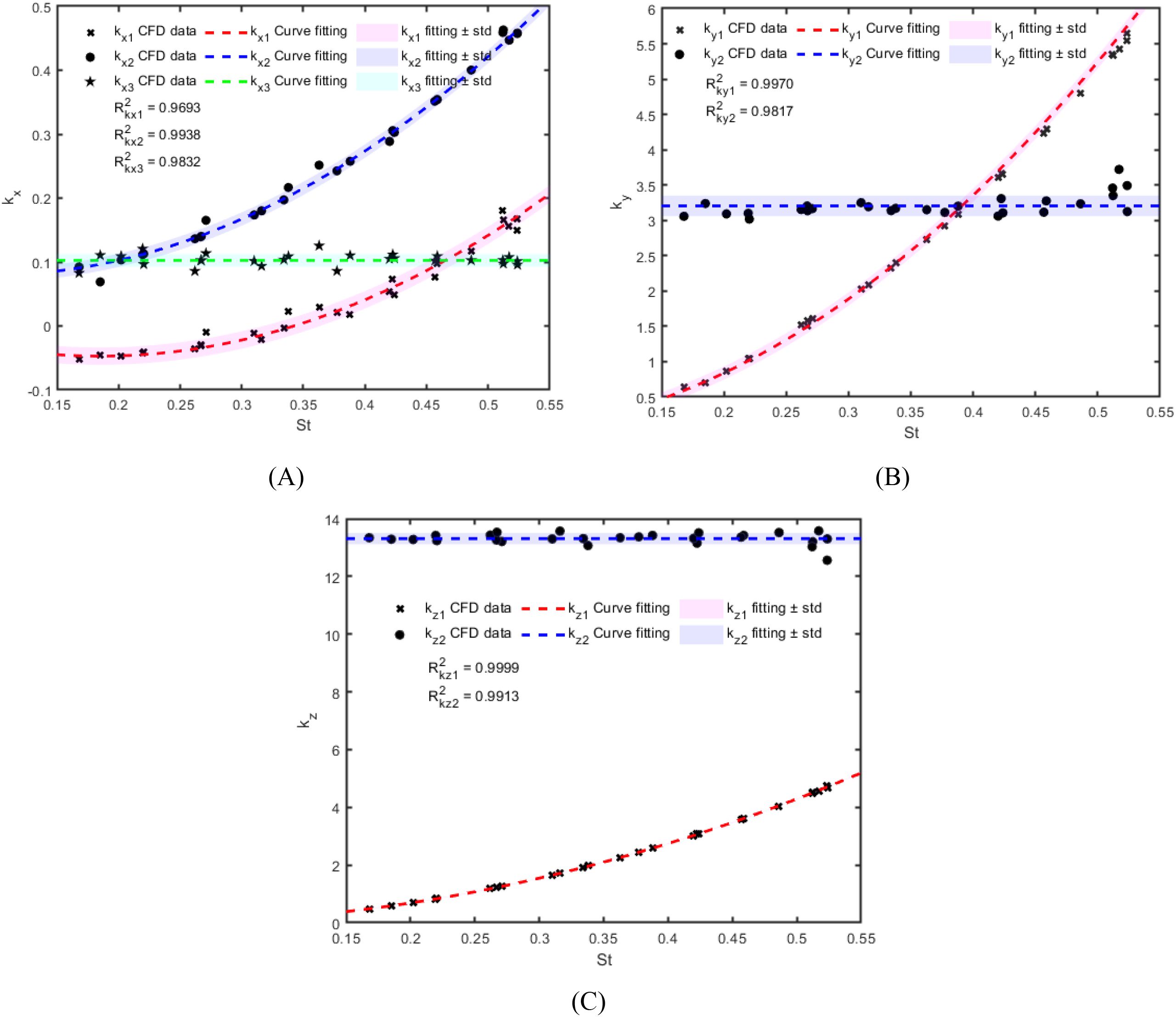
Figure 9. The variation patterns of the parameters related to the thrust coefficients of swing tail with respect to $St$. (A) Parameters related to surge thrust coefficient $C_T$; (B) Parameters related to sway force coefficient $C_L$; (C) Parameters related to yaw moment coefficient $C_M$.

In addition, if we define the overall system Reynolds number as $Re=\frac{U_{s}L}{\nu }$ (where $\nu$ is the kinematic viscosity of the fluid), the computed values listed in Appendix B span the range 10⁵~10⁶, placing the flow firmly in the fully turbulent regime. It is noteworthy that cases yielding nearly identical Strouhal numbers St can exhibit markedly different Reynolds numbers Re, whereas cases with similar Re may possess distinct St. This implies that neither St nor Re alone is sufficient to characterize the scale effects on tail-vortex dynamics and turbulent kinetic energy distribution. Consequently, when scaling prototypes up or down, simultaneous similarity in both St and Re must be maintained to reliably reproduce the thrust characteristics observed under laboratory conditions.

4.4.2.2 Propellers

By analyzing the relationship between the force ${\tau }_{\text{prop}}$ experienced by the propeller thruster, as obtained from CFD calculations, and the advance number $J$, and employing linear regression for data fitting, it is found that the thrust coefficient of propeller $K_T$ decreases with increasing advance number $J$, exhibiting an approximate linear relationship, as shown in Figure 10. The curve relationship for the thrust coefficient is given by Equation 27

Figure 10

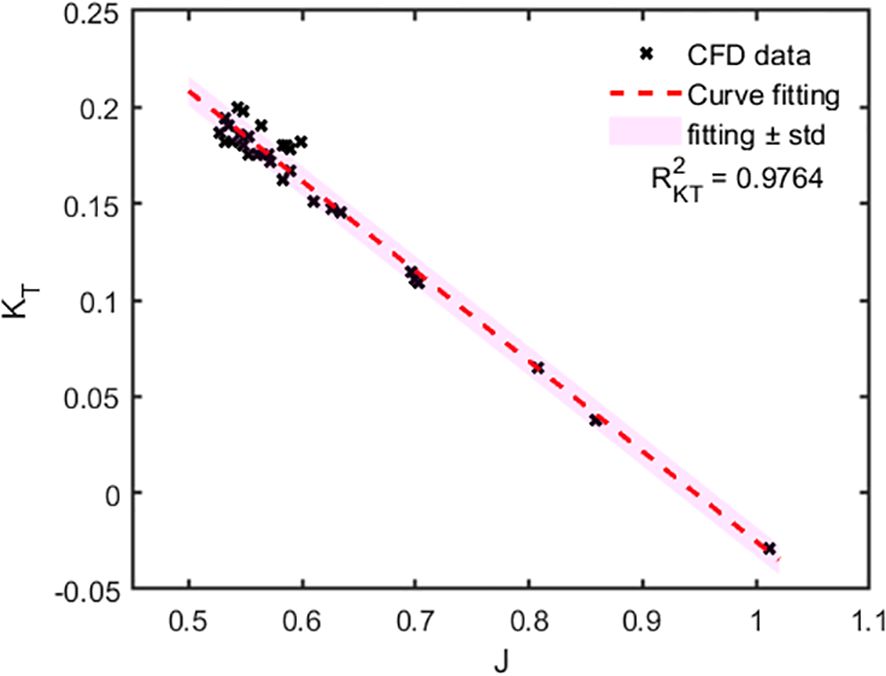
Figure 10. The variation patterns of the thrust coefficient of propeller with respect to $St$.

$\begin{array}{ll}{K}_T=-0.4674J+0.4421& (27)\end{array}$

Thus, by combining theoretical calculations and CFD simulations, we have identified the nonlinear hydrodynamic coefficients required for the dynamics model of the robotic fish, thereby fully constructing the mathematical model of the hybrid-driven robotic fish system.

5 Model validation and maneuverability analysis of simulation results

5.1 Simulation model construction

As shown in Figure 11, based on the motion equations of the hybrid-driven robotic fish derived earlier, a maneuverability simulation model was constructed in the MATLAB/Simulink environment, with its framework structure. The control input signals for the hybrid-driven robotic fish system include the swinging frequency $f$ and the swinging offset ${\theta }_{\text{offset}}$ of the three-joint tail actuator HA3; the rotational speeds $n_{\text{HA}1}$, $n_{\text{HA}2}$, and $n_{\text{VA}1}$ of the left and right horizontal propeller thrusters HA1 and HA2, and the heave propeller thruster VA1; and the angles ${\delta }_{\text{VA}2}$ and ${\delta }_{\text{VA}3}$ of the left and right pectoral fins VA2 and VA3 relative to the body. The output signals are the position and attitude vector $\eta$ and velocity vector $v$ of the robotic fish.

Figure 11

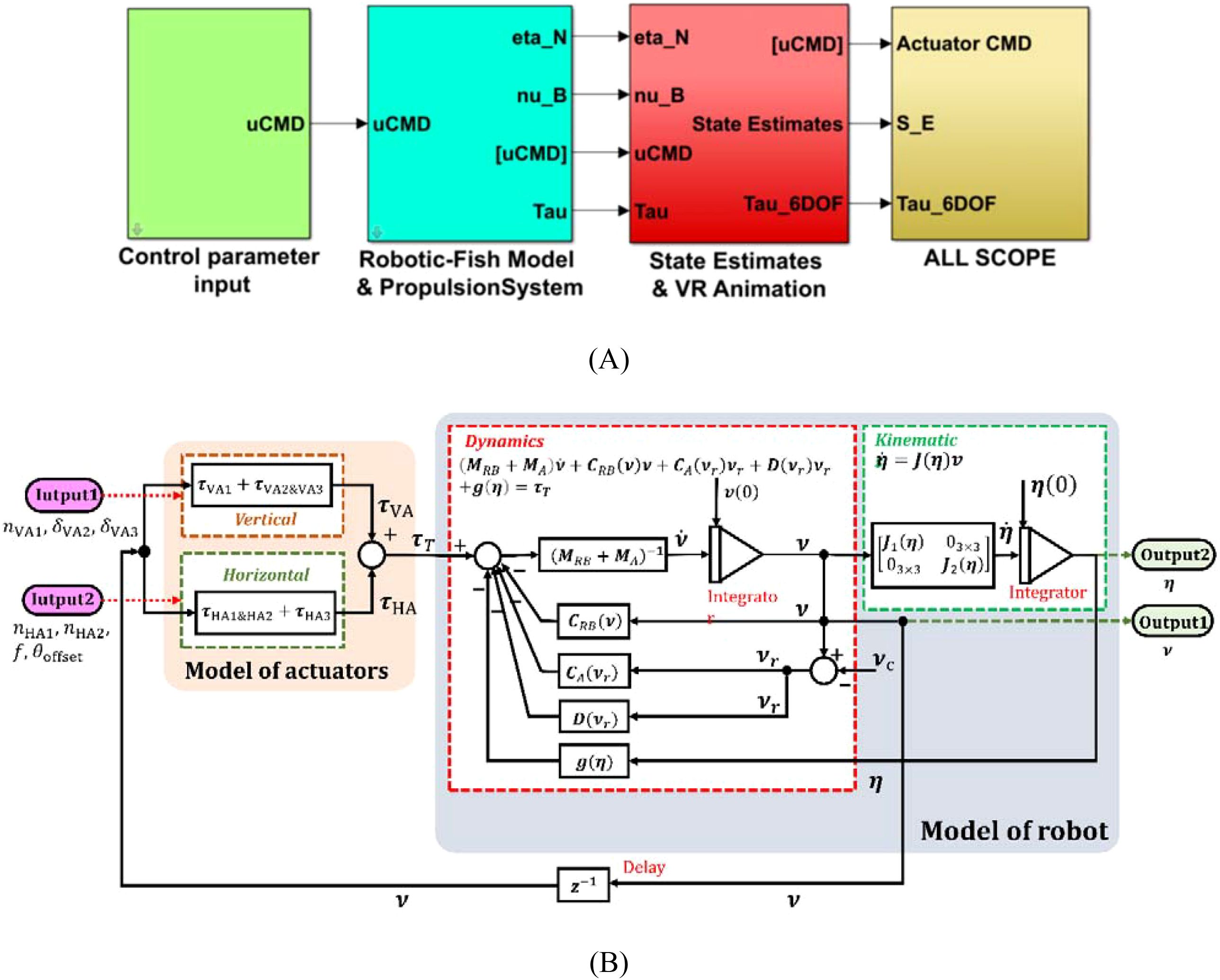
Figure 11. Maneuverability simulation model. (A) MATLAB/Simulink simulation model; (B) System simulation framework.

5.2 Maneuverability performance analysis and experimental verification

5.2.1 Surge motion speed

The surge motion swimming speed of the robotic fish directly reflects its locomotive capability. To analyze the surge speed and validate the accuracy of the simulation model, we compared the results obtained from CFD simulations, the numerical simulation model established in Simulink, and the measurements from the prototype experiments. We compared the cruising speeds of the robotic fish under both single-propulsion modes and the hybrid-drive mode.

The swimming speed measurement experiments for the robotic fish prototype were conducted in a water tank of fixed dimensions, where the swimming speed was calculated by measuring the time it took for the robotic fish to travel a fixed distance (excluding the distance covered during the initial acceleration phase). The rotation speed range of the propeller thrusters was set between 500 and 3000 rpm. To ensure that the servomotors of the swinging joints were not damaged (due to the large size of the robotic fish, a high swinging frequency would increase the hydrodynamic forces on the joints, causing the servomotors to overload), the tail swinging frequency of the prototype was limited to within 1.5 Hz. Each set of experiments was conducted six times, and the average of the measurement results was taken along with an error analysis.

As shown in Figure 12A, in the pure propeller propulsion mode, the three sets of results show good agreement. However, in the pure tail swinging mode, the CFD results overestimate the cruising speed. From the perspectives of fluid mechanics and energy conservation, the overestimation originates from an energy-budget imbalance caused by “degree-of-freedom truncation” (Liu et al., 2021). During straight-line propulsion, the periodic lateral force generated by the tail fin produces not only longitudinal thrust but also coupled yaw and sway motions. These additional degrees of freedom continuously alter the instantaneous angle of attack of the oncoming flow relative to the tail, inducing extra lateral vortex shedding and energy dissipation. In the CFD computations, however, the fish body is constrained to planar surge motion, shutting down the two aforementioned dissipation pathways. Consequently, the mechanical energy that should have been consumed by yaw and sway damping is still counted as “effective propulsive work”, thereby artificially inflating the propulsive efficiency of the tail fin. However, this does not significantly affect our study, as our focus is on the variation patterns of the hydrodynamic coefficients, rather than the motion state of the robotic fish. Within a limited range, the Simulink simulation and experimental results exhibit good consistency, which to some extent validates the reliability of the established simulation model.

Figure 12

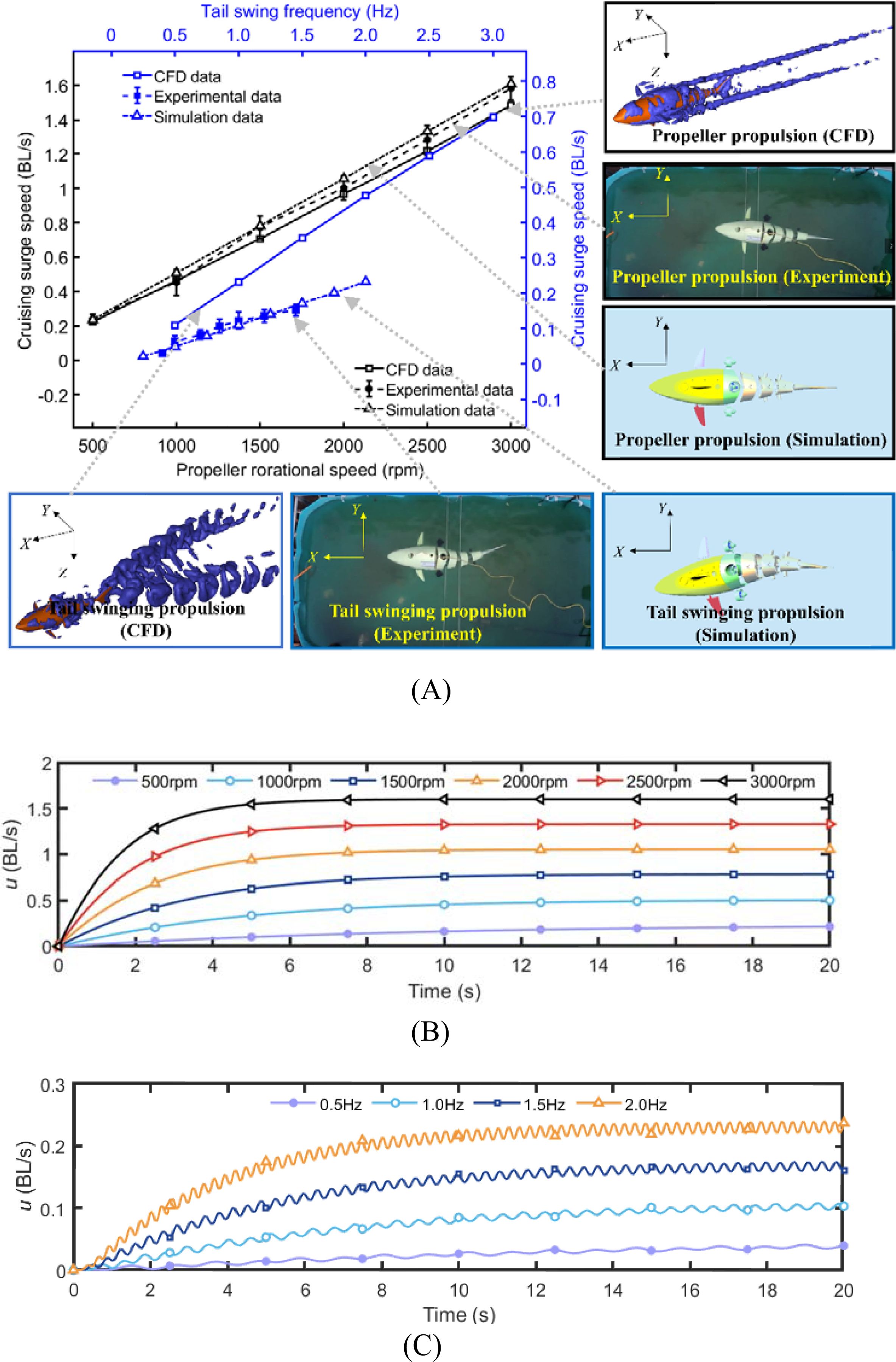
Figure 12. Comparison of simulation and experiment results under two single-propulsion modes. (A) The cruising surge speeds; (B) The instantaneous surge speed of the propeller propulsion mode; (C) The instantaneous surge speed of the tail swing propulsion mode.

Using the simulation platform, the horizontal plane instantaneous surge speed of the robotic fish was analyzed under two conditions: when propelled by the horizontal propeller thrusters and when propelled by the swinging tail. By varying the propeller rotational speed and the tail swing frequency, different swimming speeds can be achieved. Figures 12B, C display the instantaneous swimming speed curves at different propeller rotational speeds and tail swing frequencies, respectively, without underwater current disturbances. It can be observed that, under the influence of the propellers, as the rotation speed increases, the maximum surge speed that the robotic fish can achieve gradually increases, and the time required to reach this speed decreases. Within the rotation speed range of 500 to 3000 rpm, the surge speed of the robotic fish can reach 0.23 to 1.6 BL/s. Under the influence of tail swinging, as the tail swing frequency increases, the thrust provided also increases, leading to a higher achievable surge speed and a shorter time to reach this speed. Due to the periodic oscillation of the thrust from the three-joint tail propulsion system, the instantaneous swimming speed of the robotic fish exhibits periodic oscillation. Within the tail swing frequency range of 0.5 to 2 Hz, the surge motion speed of the robotic fish can reach 0.04 to 0.23 BL/s.

During hybrid-driven trials, both Simulink simulations and prototype tests revealed that the robotic fish suffered from poor straight-line stability caused by persistent yaw motion. This issue became most pronounced when high propeller speeds were paired with low tail-beat frequencies. According to the preceding CFD analysis, this occurs because the Strouhal number falls below 0.33, so the tail generates virtually no useful thrust while its lateral sweeps still produce yawing moments. These moments interact with the surge force delivered by the propellers, causing the yaw angle to accumulate and the vehicle to drift off the intended straight path. Figure 13 compares the cruising speeds achieved in hybrid mode for tail swing frequencies of 1 Hz and 1.5 Hz within a limited propeller-speed envelope. Simulink predictions and experimental data agree closely, whereas CFD again slightly overestimates the speed. Under conditions that still allow straight-line swimming, a tail swing frequency of 1.5 Hz combined with a propeller speed of 1500 rpm yields approximately 0.63 BL/s.

Figure 13

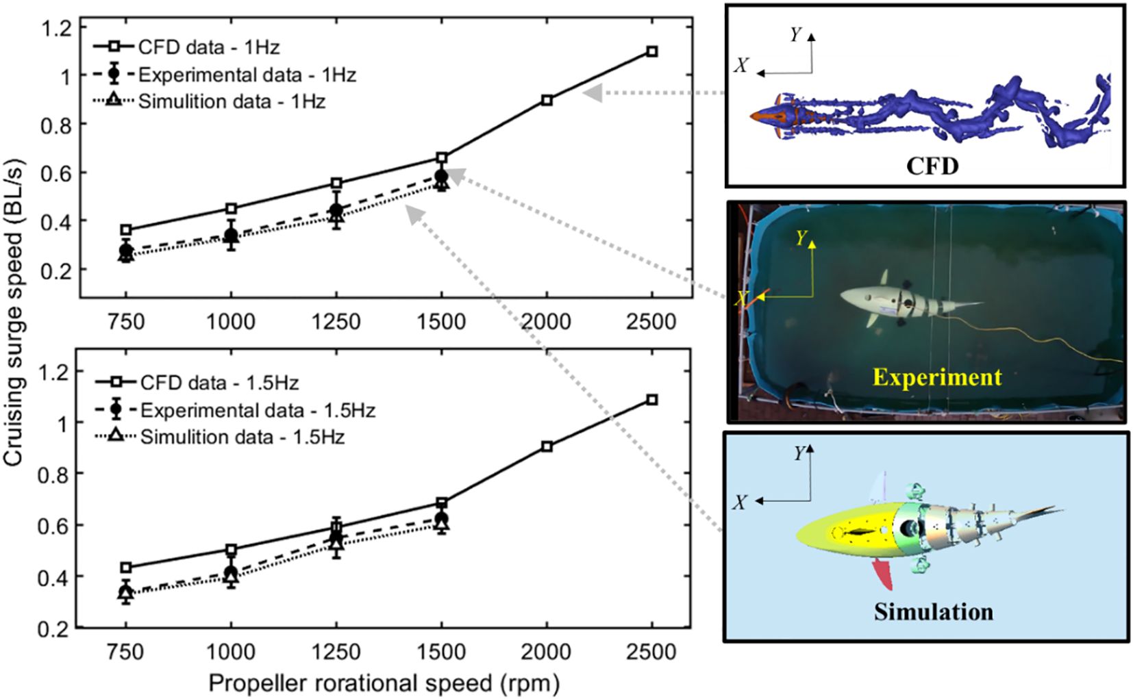
Figure 13. Comparison of simulation and experiment results under hybrid-drive mode.

5.2.2 Minimum turning radiuses

The minimum turning radius of the robotic fish reflects its maneuverability and flexibility. There are four ways to achieve planar turning motion for the robotic fish: 1) Pure tail swinging: The tail swings asymmetrically along the fish’s tail, with the horizontal thrusters turned off; 2) Pure propeller propulsion: The two propeller thrusters rotate at different speeds, with no tail swinging; 3) Hybrid drive method A: The tail swings symmetrically, and the horizontal propeller thrusters rotate at different speeds; 4) Hybrid drive method B: The tail swings asymmetrically, and the horizontal propeller thrusters rotate at the same speed. The results of methods 1 and 2 represent the minimum turning radii of the robotic fish in two single modes, while the results of methods 3 and 4 will not be smaller than those of method 2. The maximum tail swing offset of the robotic fish is set to 45°, and the maximum differential speed of the two horizontal thrusters is 3000 rpm (the upper limit of the thruster speed). As shown in Figure 14A, in an outer lake, the circular motion of the robotic fish moving with the maximum tail swing offset at different swinging frequencies or with different differential speeds of the horizontal propeller thrusters (with one propeller thruster rotational speed at 0) is tested and analyzed, without underwater current disturbances. The experimental and simulation results are presented in Figures 14B, C. In the pure tail swinging mode, the turning radius of the robotic fish moving with the maximum tail swing offset at different swinging frequencies is very close, with the minimum value being around 2.9 BL at a swinging frequency of 1 Hz. In the pure propeller propulsion mode, the turning radius decreases as the speed difference between the two horizontal thrusters increases, with the minimum value being around 0.6 BL at a speed difference of 3000 rpm. It is evident that the differential rotation of the two horizontal propellers enables the robotic fish to have a smaller turning radius, indicating stronger maneuverability and flexibility.

Figure 14

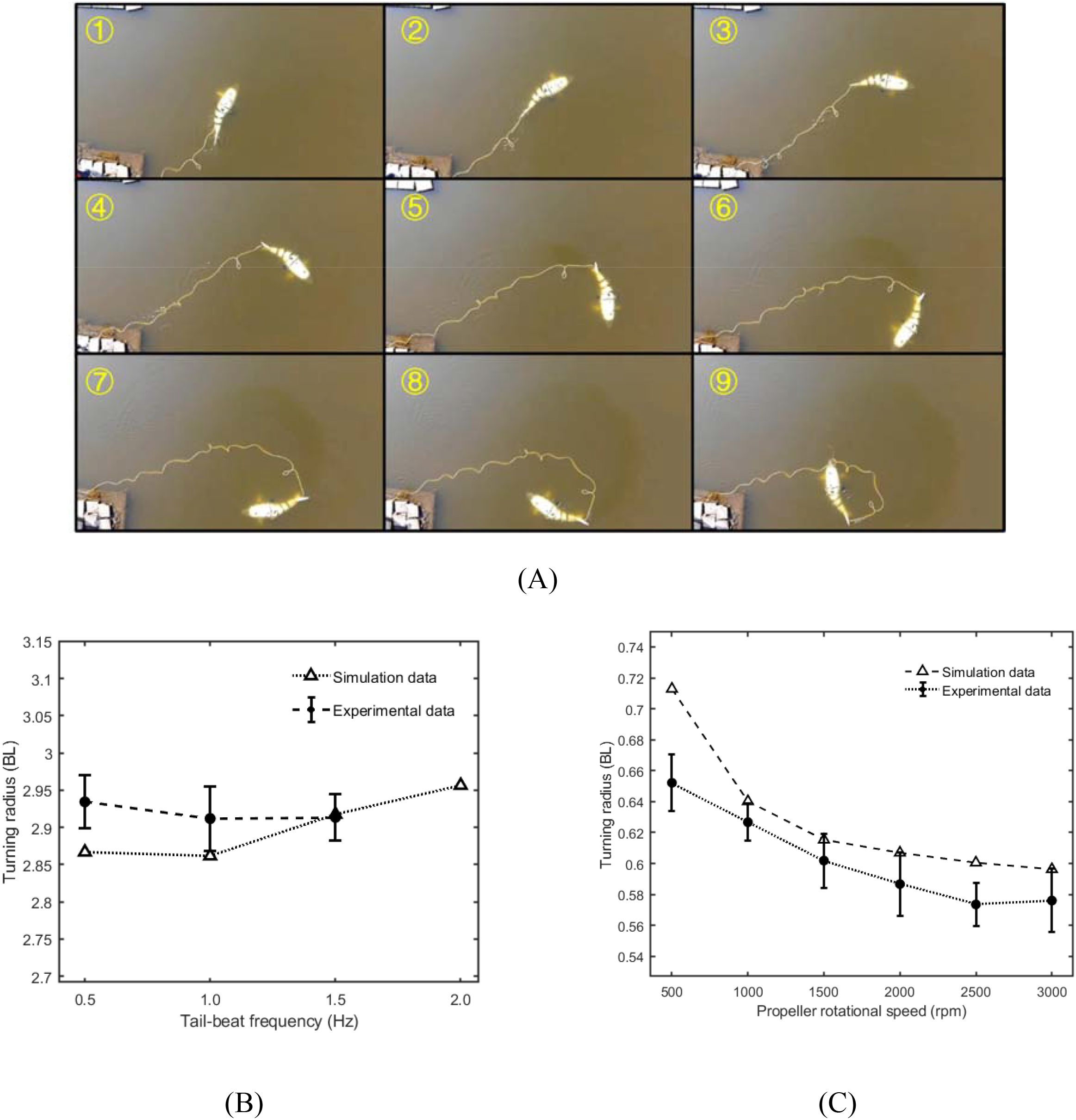
Figure 14. Circular-turn trajectories of the robotic fish. (A) Overview of the swimming sequence; (B) Turning radius with the maximum tail-swing offset at various beating frequencies; (C) Turning radius under different differential thrust settings of the horizontal propellers.

5.2.3 Motion characteristics in the 3D space

In addition to testing the aforementioned planar motion metrics, the robotic fish we developed also possesses the capability for 3D spatial motion. By utilizing its heave propeller and pectoral fin rotation, it can generate heave forces and moments, thereby enabling its movement in the vertical plane. Due to experimental constraints (lack of underwater filming equipment), we only verified the robotic fish’s diving and surfacing capabilities, as shown in Figure 15.

Figure 15

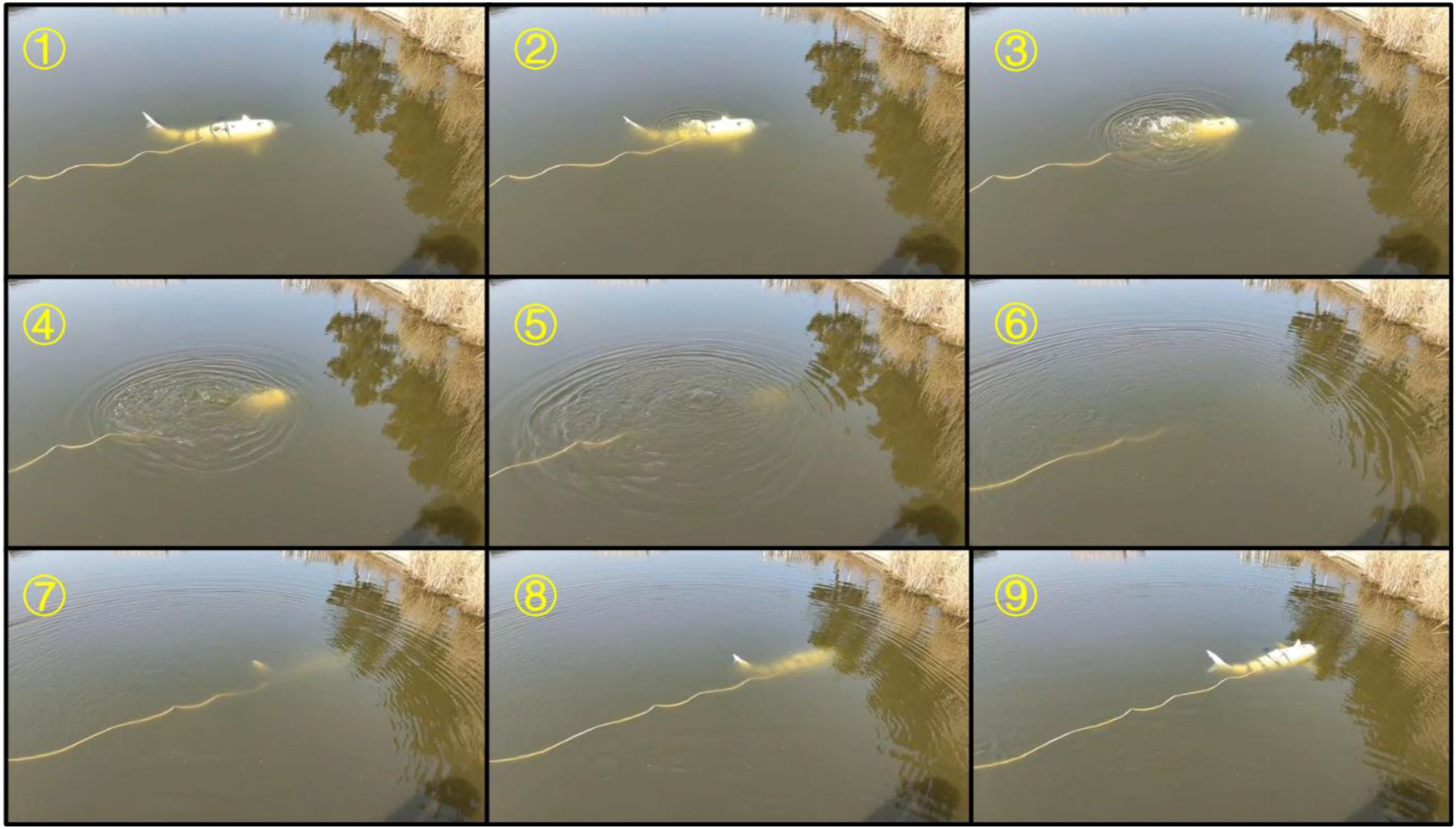
Figure 15. The submerged movement of the robotic fish.

To demonstrate the capability for 3D spatial motion, we have also utilized the Virtual Reality Simulation module in Matlab/Simulink to visualize the motion of the robotic fish, as shown in Figure 16. We have presented several typical motion scenarios of the robotic fish, including 3D helical motion, right-angle motion in the vertical plane, and “V”-shaped diving and surfacing motion. Specifically, Figure 16A shows the robotic fish moving in the biomimetic propulsion mode, with a simulation duration $T_1=180$ s, and simulation inputs of swinging frequency f = 2 Hz, swinging offset ${\theta }_{\text{offset}}=45°$, and pectoral fin angles ${\delta }_{\text{VA}1}={\delta }_{\text{VA}2}=30°$. Figure 16B illustrates the robotic fish moving in the propeller propulsion mode, with a simulation duration $T_2=100$ s, and simulation inputs for the propeller speeds $n_{\text{HA}1}=n_{\text{HA}2}=500u(t)$ rpm, $n_{\text{VA}1}=500[1-u(t)]$ rpm, where $u(t)$ is a unit step function with a step time of $0.5T_2$. Figure 16C depicts the robotic fish moving in the hybrid-driven mode, with a simulation duration $T_3=100$ s, where the horizontal thrusters provide thrust for straight-line motion, and the pectoral fin rotation provides heave force for vertical diving and surfacing. The simulation inputs are the speeds of the two horizontal propeller thrusters $n_{\text{HA}1}=n_{\text{HA}2}=500$ rpm, and the pectoral fin angles ${\delta }_{\text{VA}1}={\delta }_{\text{VA}2}=60°[2\delta (t)-1]$, where $\delta (t)$ is a unit pulse function with a period of $T_3$ and a pulse width of $0.5T_3$. By activating different motion actuators of the hybrid-driven robotic fish, various motion states can be achieved, demonstrating the robotic fish’s excellent 3D motion performance.

Figure 16

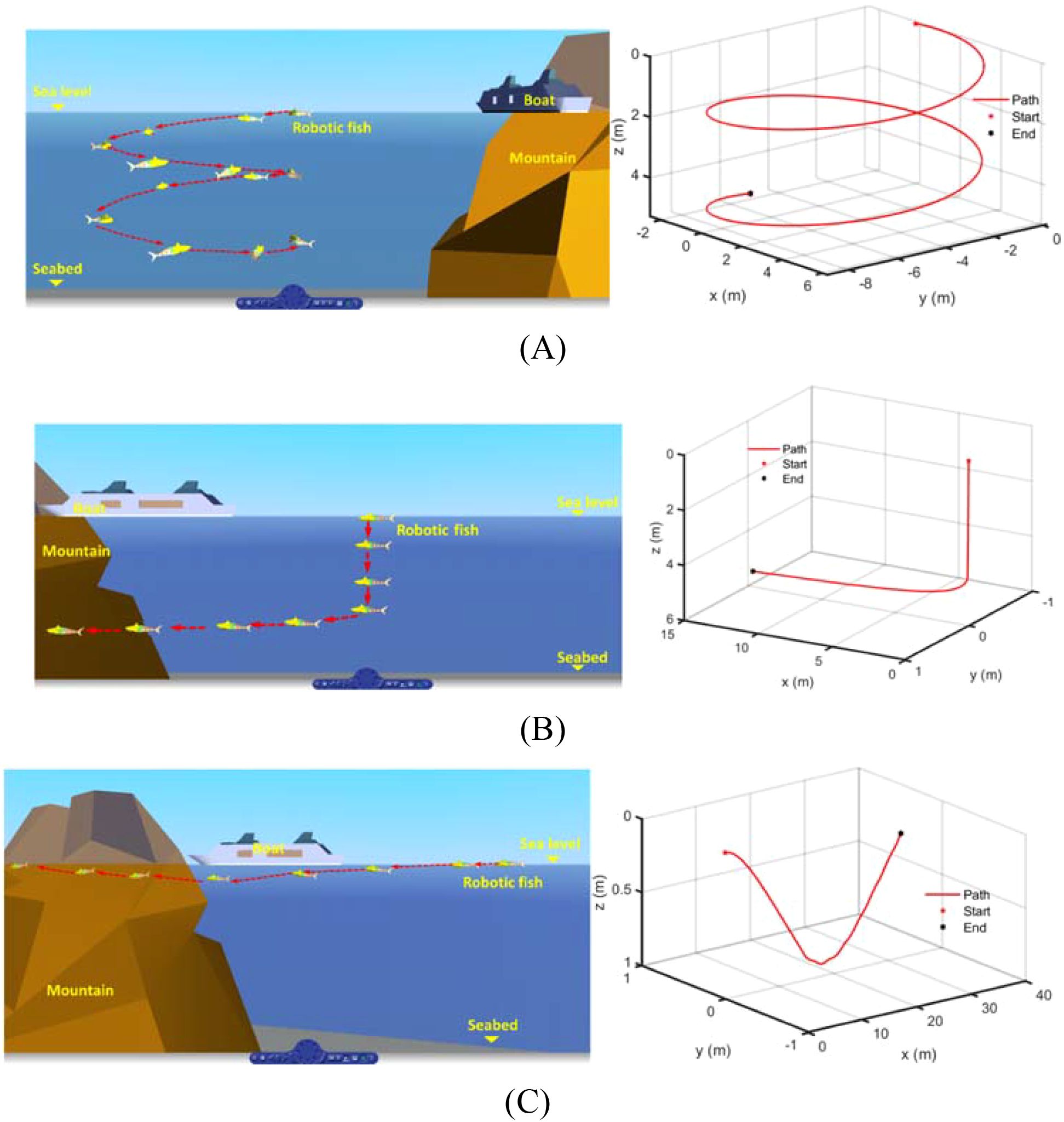
Figure 16. The typical motion scenarios. (A) Movement in the biomimetic propulsion mode; (B) Movement in the propeller propulsion mode; (C) Movement in the hybrid-driven mode.

5.3 Uncertainty analysis of hydrodynamic coefficients

Ocean-current disturbances and other stochastic environmental factors introduce parametric uncertainties that perturb the system’s hydrodynamic coefficients. To further investigate the influence of these coefficients on the system’s dynamic performance under uncertain disturbances, we introduced a time-varying random noise with an amplitude not exceeding ±10% of the original coefficient, based on these coefficients obtained from CFD simulations. This perturbation of the hydrodynamic parameters aims to quantify the influence of uncertainties on the hydrodynamic coefficients and to further analyze their influence on the system dynamic output. The specific procedures are as follows: (1) Added-mass coefficients: perturbation limits are set as a fixed base value scaled by a prescribed percentage and superimposed on the original coefficients. (2) Damping coefficients: linear and quadratic nominal values are scaled by the same percentage to generate perturbation limits, which are then added to the original coefficients. (3) Propeller thrust coefficient $K_T$: constant coefficients (–0.4674 and 0.4421) scaled by the prescribed percentage define the perturbation limits, which are then added on the original coefficient. (4) Tail thrust coefficients $C_T$, $C_L$, and $C_M$: perturbation limits are set as the current nominal values scaled by the prescribed percentage and added to the original coefficients.

Taking the planar straight-line swimming motion of the robotic fish as an example, the influence of hydrodynamic coefficients perturbation on the surge speed of the robotic fish is analyzed under two single propulsion modes. For the propeller propulsion mode and the tail swinging propulsion mode, the control commands for the actuators are respectively set to $n_{\text{HA}1}=n_{\text{HA}2}=2000$ rpm and $f=2\text{Hz}$, with all other parameters set to 0. As shown in Figures 17, 18, within the range of parameter perturbation, the surge speed $u$ in the propeller propulsion mode remains essentially consistent with that without parameter perturbation, exhibiting only minor fluctuations. In contrast, under the tail swinging propulsion mode, as the parameter perturbation intensifies, the fluctuation range of the surge speed significantly increases. Meanwhile, this observation indicates that within the same level of parametric perturbation, the variation in surge speed is more pronounced in the tail swinging propulsion mode. Therefore, when environmental disturbances are significant and thrust coefficient perturbation is severe, it is advisable to employ the propeller propulsion mode rather than the tail swinging propulsion mode to ensure the stability of the robotic fish’s motion.

Figure 17

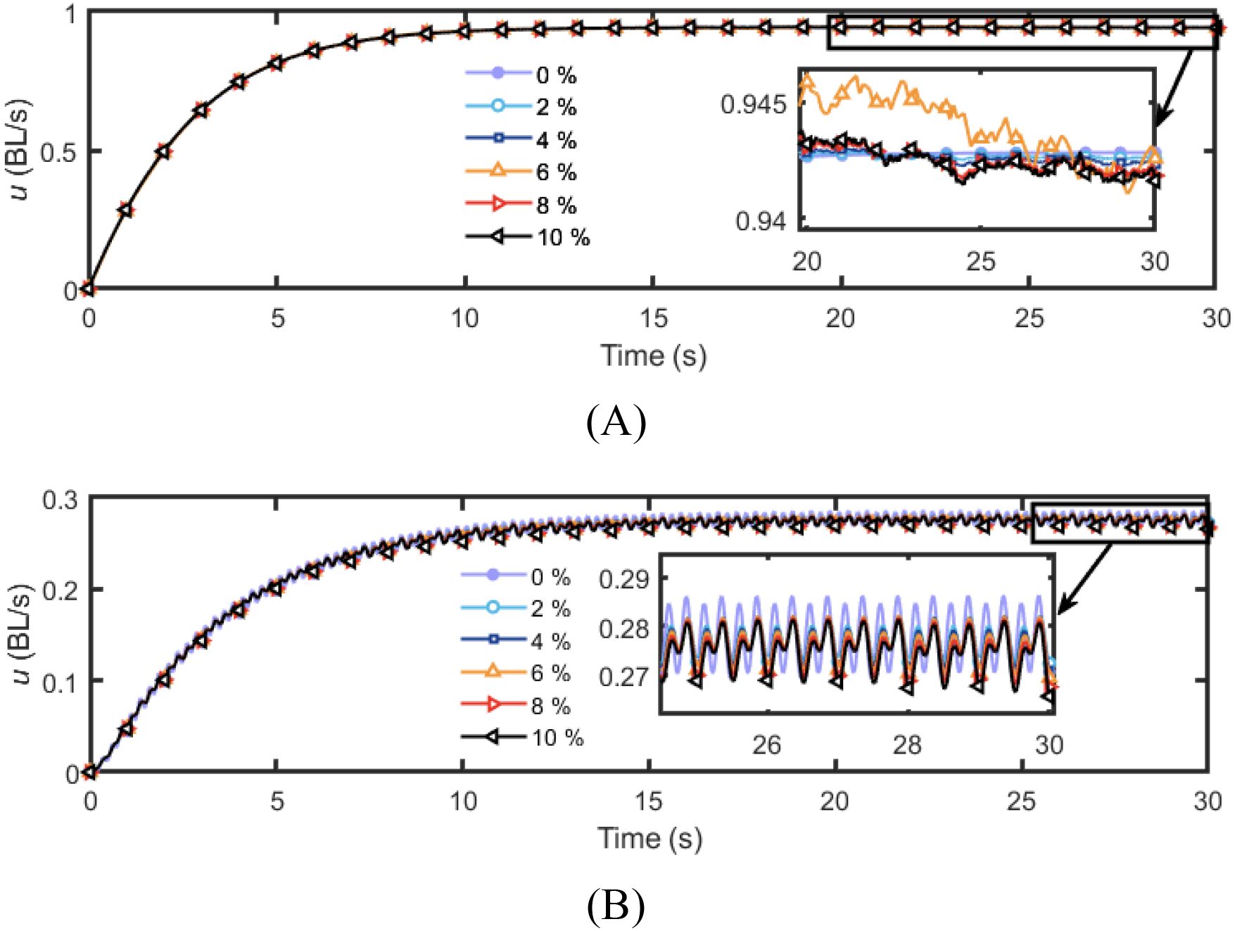
Figure 17. Influence of perturbations in Radiation-induced force coefficients on surge speed. (A) Propeller propulsion mode; (B) Tail swinging propulsion mode.

Figure 18

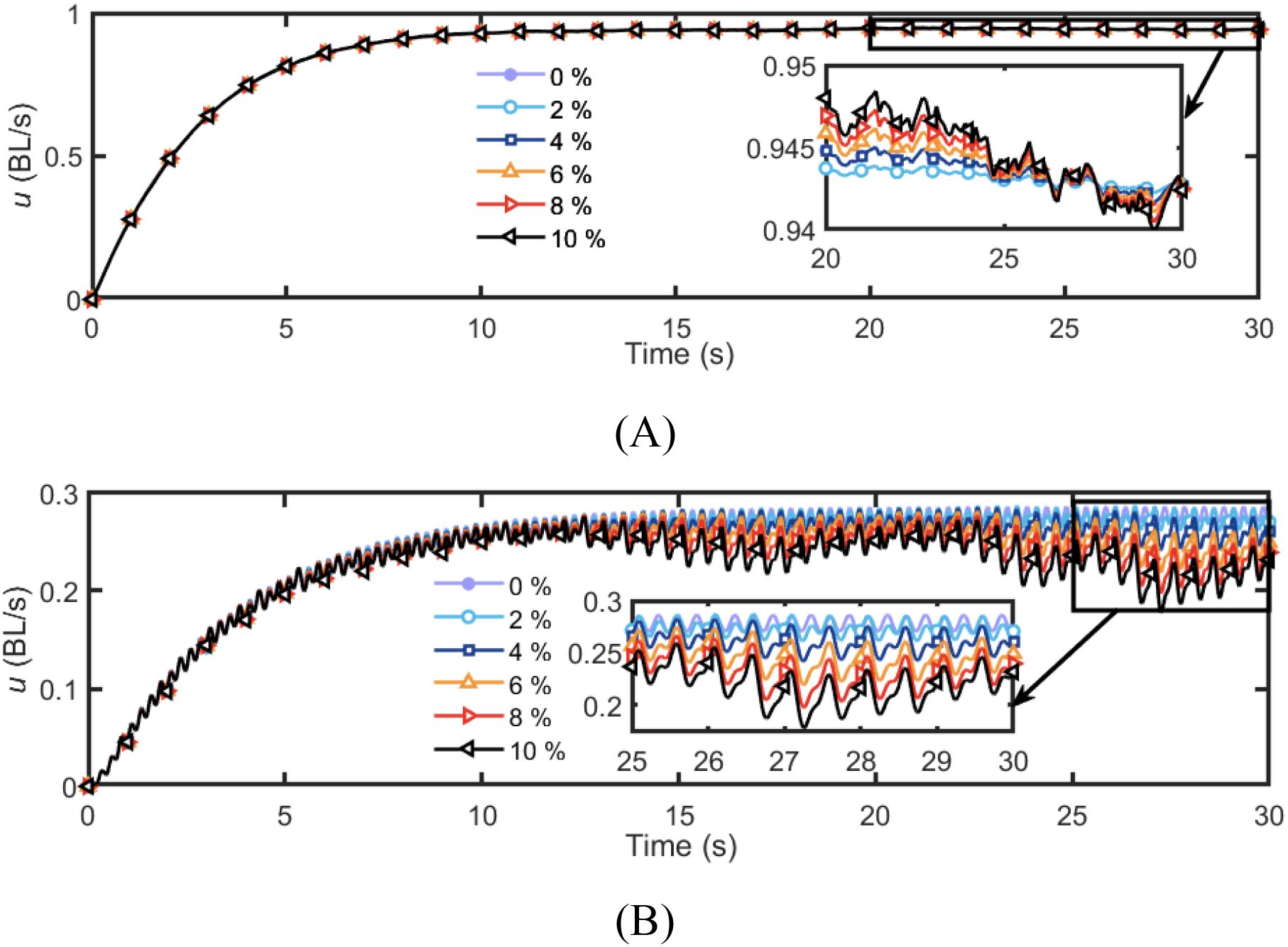
Figure 18. Influence of perturbations in thrust coefficients on surge speed. (A) Propeller propulsion mode; (B) Tail swinging propulsion mode.

6 Conclusion

This study conducted mathematical modeling, prototype testing and maneuverability simulation based on the proposed hybrid-driven robotic. The conclusions of the work are as follows.

1. A hybrid-driven robotic fish equipped with both biomimetic fin and propeller propulsion was designed and manufactured. Considering the effects of added mass forces and fluid damping forces, a coupled mathematical model of hydrodynamics and mechanical dynamics for the hybrid-driven robotic fish was established based on classical rigid body dynamics theory.

2. A numerical simulation model of the robotic fish was established using 3D modeling and CFD simulation software. Hydrodynamic data fitting method was used to obtain the hydrodynamic damping coefficient of the robotic fish’s body, the thrust coefficient of the swing tail, and the thrust coefficient of propeller, thereby supplementing and perfecting the dynamics model of the hybrid-driven robotic fish. It was found that the surge thrust coefficient $C_T$, sway force coefficient $C_L$, and yaw moment coefficient $C_M$ of the robotic fish’s three-joint tail can all be fitted as explicit functions related to the tail swing frequency f and the Strouhal number St in the time domain. When St< 0.33, the tail cannot provide effective positive thrust. The thrust coefficient of propeller $K_T$ was approximately linearly negatively correlated with the advance number J, consistent with the characteristic curve of the propeller.

3. By comparing the CFD calculation results, Simulink simulation results, and prototype test results for the multiple motion state of the robotic fish, a MATLAB/Simulink simulation platform for the motion of the hybrid-driven robotic fish was constructed and validated. Based on the simulation platform, the locomotive capabilities and maneuverability of the robotic fish were analyzed. In the propeller propulsion mode, within the horizontal propeller rotation speed range from 500 rpm to 3000 rpm, the straight-line speed of the robotic fish can reach from 0.23 BL/s to 1.6 BL/s, and the minimum turning radius can be 0.6 BL when the speed difference between the two propellers was 3000 rpm. In the tail swing drive mode, within the tail swing frequency range from 0.5 Hz to 2 Hz, the straight-line speed of the robotic fish can reach from 0.04 to 0.23 BL/s, and the minimum turning radius can be 2.9 BL at the tail swing frequency of 1 Hz. Additionally, several typical 3D spatial motion scenarios were designed using the three drive modes of the robotic fish, and virtual reality techniques were employed for visualization, demonstrating the 3D spatial motion capabilities of the hybrid-driven robotic fish.

Moreover, the influence of perturbations in hydrodynamic coefficients on surge speed was analyzed based on the simulation platform. The results indicated that the propeller mode exhibits markedly superior robustness to parameter perturbations compared with the tail swing mode, making it the preferred configuration for deployment in highly disturbed underwater environments.

This research provides valuable insights into the exploration and design of new types of high-performance and efficient biomimetic underwater robots, primarily addressing the dynamics analysis, hydrodynamic coefficient identification, and open-loop manipulation system simulation modeling issues of the hybrid-driven robotic fish. Furthermore, the rationality and effectiveness of the dynamics model are validated through the simulation analysis and prototype testing of the robotic fish’s motion state, laying the groundwork and theoretical foundation for further research on the complex closed-loop system motion control of the hybrid-driven robotic fish.

Building on this foundation, our future work will concentrate on guidance and motion control of the robotic fish: constructing a state observer for real-time motion estimation and feedback generation; dynamically allocating control inputs for the under-actuated system based on guidance laws; and devising mode-switching strategies together with dedicated controllers. The ultimate goal is to achieve high-precision, high-efficiency closed-loop path/trajectory tracking for the hybrid-driven robotic fish in complex environments.

Data availability statement

The datasets presented in this study can be found in online repositories. The names of the repository/repositories and accession number(s) can be found below: https://github.com/Baifagang/Hybrid-Driven-Robotic-fish-Simulator.

Author contributions

FB: Software, Formal Analysis, Visualization, Validation, Data curation, Conceptualization, Writing – original draft, Methodology. XS: Methodology, Writing – review & editing, Investigation. ZW: Software, Writing – review & editing, Validation. XW: Validation, Writing – review & editing, Formal Analysis. YL: Writing – review & editing, Methodology. KL: Validation, Writing – review & editing, Software. GX: Funding acquisition, Writing – review & editing, Project administration.

Funding

The author(s) declare financial support was received for the research and/or publication of this article. This work is supported by the National Key Research and Development Program of China (2023YFC2810100), the National Natural Science Foundation of China (52471331).

Acknowledgments

The authors would like to express their sincere gratitude to the National Key Research and Development Program of China (2023YFC2810100) and the National Natural Science Foundation of China (52471331) for their financial support.

Conflict of interest

The authors declare that the research was conducted in the absence of any commercial or financial relationships that could be construed as a potential conflict of interest.

Generative AI statement

The author(s) declare that no Generative AI was used in the creation of this manuscript.

Any alternative text (alt text) provided alongside figures in this article has been generated by Frontiers with the support of artificial intelligence and reasonable efforts have been made to ensure accuracy, including review by the authors wherever possible. If you identify any issues, please contact us.

Publisher’s note

All claims expressed in this article are solely those of the authors and do not necessarily represent those of their affiliated organizations, or those of the publisher, the editors and the reviewers. Any product that may be evaluated in this article, or claim that may be made by its manufacturer, is not guaranteed or endorsed by the publisher.

Supplementary material

The Supplementary Material for this article can be found online at: https://www.frontiersin.org/articles/10.3389/fmars.2025.1648335/full#supplementary-material

References

Ahmad Mazlan A. N. (2015). A fully actuated tail propulsion system for a biomimetic autonomous underwater vehicle (Glasgow, UK: University of Glasgow). Available online at: https://theses.gla.ac.uk/6343/ (Accessed April 3, 2025).

Google Scholar

Barrett D., Grosenbaugh M., and Triantafyllou M. (1996). “The optimal control of a flexible hull robotic undersea vehicle propelled by an oscillating foil,” in Proceedings of symposium on autonomous underwater vehicle technology (IEEE, USA), 1–9. doi: 10.1109/AUV.1996.532833

Crossref Full Text | Google Scholar

Borazjani I. and Sotiropoulos F. (2008). Numerical investigation of the hydrodynamics of carangiform swimming in the transitional and inertial flow regimes. J. Exp. Biol. 211, 1541–1558. doi: 10.1242/jeb.015644

PubMed Abstract | Crossref Full Text | Google Scholar

Chen Y., Qiao J., Liu J., Zhao R., An D., and Wei Y. (2022). Three-dimensional path following control system for net cage inspection using bionic robotic fish. Inf. Process. Agric. 9, 100–111. doi: 10.1016/j.inpa.2021.12.002

Crossref Full Text | Google Scholar

Chen D., Wu Z., Meng Y., Tan M., and Yu J. (2022). Development of a high-speed swimming robot with the capability of fish-like leaping. IEEE/ASME Trans. Mechatron. 27, 3579–3589. doi: 10.1109/TMECH.2021.3136342

Crossref Full Text | Google Scholar

Fahrni L., Thies P. R., Johanning L., and Cowles J. (2018). “Scope and feasibility of autonomous robotic subsea intervention systems for offshore inspection, maintenance and repair,” in Renewable energies offshore proceedings of the 3rd international conference on renewable energies offshore (RENEW 2018) (CRC Press-Taylor & Francis, London), 771–778. doi: 10.1201/9780429505324

Crossref Full Text | Google Scholar

Fossen T. L. (1994). Guidance and control of ocean vehicles (New York: Wiley).

Google Scholar

Gong Q., Zhang W., Su Y., and Yang H. (2024). Guidance and control of underwater hexapod robot based on adaptive sliding mode strategy. J. Bionic Eng. 22, 118–132. doi: 10.1007/s42235-024-00625-0

Crossref Full Text | Google Scholar

Hu J., Xiao Q., and Li R. (2021). Numerical simulation of a multi-body system mimicking coupled active and passive movements of fish swimming. J. Mar. Sci. Eng. 9, 334. doi: 10.3390/jmse9030334

Crossref Full Text | Google Scholar

Huang H., Xian S., Xiong C., Li W., and Zhong Y. (2025). Design and dynamics modeling of a hybrid drive bionic robotic fish. Biomimetic Intell. Robotics, 100247. doi: 10.1016/j.birob.2025.100247

Crossref Full Text | Google Scholar

Ji Y., Wei Y., Liu J., and An D. (2023). Design and realization of a novel hybrid-drive robotic fish for aquaculture water quality monitoring. J. Bionic Eng. 20, 543–557. doi: 10.1007/s42235-022-00282-1

Crossref Full Text | Google Scholar

Li C., Guo S., and Guo J. (2022). Performance evaluation of a hybrid thruster for spherical underwater robots. IEEE Trans. Instrum. Meas. 71, 1–10. doi: 10.1109/TIM.2022.3178700

Crossref Full Text | Google Scholar

Li S., Wu Z., Dai S., Wang J., Tan M., and Yu J. (2024). Tight-space maneuvering of a hybrid-driven robotic fish using backstepping-based adaptive control. IEEE/ASME Trans. Mechatron. 29, 3219–3231. doi: 10.1109/TMECH.2023.3338879

Crossref Full Text | Google Scholar

Liljeback P. and Mills R. (2017). “Eelume: A flexible and subsea resident IMR vehicle,” in Oceans 2017-aberdeen (IEEE, USA), 1–4. doi: 10.1109/OCEANSE.2017.8084826

Crossref Full Text | Google Scholar

Liu J., Möller M., and Schuttelaars H. M. (2021). Balancing truncation and round-off errors in FEM: One-dimensional analysis. J. Comput. Appl. Math. 386, 113219. doi: 10.1016/j.cam.2020.113219

Crossref Full Text | Google Scholar

Liu K., Wang H., Xu X., Song T., and Meng Q. (2022). Development and trials of a novel deep-sea multi-joint autonomous underwater vehicle. Ocean Eng. 265, 112558. doi: 10.1016/j.oceaneng.2022.112558

Crossref Full Text | Google Scholar

Liu J., Yu F., He B., and Yan T. (2022). Hydrodynamic numerical simulation and prediction of bionic fish based on computational fluid dynamics and multilayer perceptron. Eng. Appl. Comp. Fluid Mech. 16, 858–878. doi: 10.1080/19942060.2022.2052355

Crossref Full Text | Google Scholar

Ozmen Koca G., Bal C., Korkmaz D., Bingol M. C., Ay M., Akpolat Z. H., et al. (2018). Three-dimensional modeling of a robotic fish based on real carp locomotion. Appl. Sci. 8, 180. doi: 10.3390/app8020180

Crossref Full Text | Google Scholar

Qiu H., Chen L., Ma X., Bi S., Wang B., and Li T. (2023). Analysis of heading stability due to interactions between pectoral and caudal fins in robotic boxfish locomotion. J. Bionic Eng. 20, 390–405. doi: 10.1007/s42235-022-00271-4

Crossref Full Text | Google Scholar

Salazar R., Fuentes V., and Abdelkefi A. (2018). Classification of biological and bioinspired aquatic systems: A review. Ocean Eng. 148, 75–114. doi: 10.1016/j.oceaneng.2017.11.012

Crossref Full Text | Google Scholar

Scaradozzi D., Palmieri G., Costa D., Zingaretti S., Panebianco L., Ciuccoli N., et al. (2017). UNIVPM BRAVe: A hybrid propulsion underwater research vehicle. Int. J. Autom. Tech. 11, 404–414. doi: 10.20965/ijat.2017.p0404

Crossref Full Text | Google Scholar

Sfakiotakis M., Lane D. M., and Davies J. B. C. (2002). Review of fish swimming modesfor aquatic locomotion. IEEE J. Ocean Eng. 24, 237–252. doi: 10.1109/48.757275

Crossref Full Text | Google Scholar

Suebsaiprom P. and Lin C. L. (2015). Maneuverability modeling and trajectory tracking for fish robot. Control Eng. Pract. 45, 22–36. doi: 10.1016/j.conengprac.2015.08.010

Crossref Full Text | Google Scholar

Terracciano D. S., Bazzarello L., Caiti A., Costanzi R., and Manzari V. (2020). Marine robots for underwater surveillance. Curr. Robot Rep. 1, 159–167. doi: 10.1007/s43154-020-00028-z

Crossref Full Text | Google Scholar

Triantafyllou G. S. M. S. (1993). Optimal thrust development inoscillating foils with application to fishpropulsion. J. Fluids Struct. 7, 205–224. doi: 10.1006/jfls.1993.1012

Crossref Full Text | Google Scholar

Versteeg H. K. and Malalasekera W. (2007). An introduction to computational fluid dynamics. Pearson Schweiz Ag 20, 400. doi: 10.1016/j.enganabound.2004.05.002

Crossref Full Text | Google Scholar

Watts C., McGookin E., and Macauley M. (2007). “Modelling and control of a biomimetic underwater vehicle with a tendon drive propulsion system,” in OCEANS 2007 – europe (IEEE, USA), 1–6. doi: 10.1109/OCEANSE.2007.4302245

Crossref Full Text | Google Scholar

Xia X., Hu N., Liu J., Chen G., Yang Q., and Chen Y. (2021). Development and innovative design research of underwater bionic fish products under hybrid propulsion technology. Wireless Commun. Mobile Computing 2021, 5146992. doi: 10.1155/2021/5146992

Crossref Full Text | Google Scholar

Xue G., Bai F., Guo L., Ren P., and Liu Y. (2023). Research on the effects of complex terrain on the hydrodynamic performance of a deep-sea fishlike exploring and sampling robot moving near the sea bottom. Front. Mar. Sci. 10. doi: 10.3389/fmars.2023.1091523

Crossref Full Text | Google Scholar

Xue G., Liu Y., Si W., Xue Y., Guo F., and Li Z. (2020). Evolvement rule and hydrodynamic effect of fluid field around fish-like model from starting to cruising. Eng. Appl. Comp. Fluid Mech. 14, 580–592. doi: 10.1080/19942060.2020.1734095

Crossref Full Text | Google Scholar

Yu Y. and Huang K. (2021). Scaling law of fish undulatory propulsion. Phys. Fluids 33, 061905. doi: 10.1063/5.0053721

Crossref Full Text | Google Scholar

Yu J., Wang T., Wu Z., and Tan M. (2019). Design of a miniature underwater angle-of-attack sensor and its application to a self-propelled robotic fish. IEEE J. Ocean Eng. 45, 1295–1307. doi: 10.1109/JOE.2019.2940800

Crossref Full Text | Google Scholar

Yuan J., Wu Z., Yu J., and Tan M. (2017). Sliding mode observer-based heading control for a gliding robotic dolphin. IEEE Trans. Ind. Electron. 64, 6815–6824. doi: 10.1109/TIE.2017.2674606

Crossref Full Text | Google Scholar

Zhao X., Jin S., Bian G., Cui Y., Wang J., Tang Y., et al. (2023). Technical design and data analysis of autonomous underwater vehicle-based side-scan sonar operations. J. Mar. Sci. Eng. 11, 2089. doi: 10.3390/jmse11112089

Crossref Full Text | Google Scholar