Chronicles in ivory: estimating the age of narwhals (Monodon monoceros) through stochastic modeling of seasonally varying trace elements

Introduction: Age estimation is an important tool for understanding the life history of animal populations, and several techniques have been developed, each with its own strengths and limitations.

Methods: In this study, we apply a novel age estimation method that utilizes trace element signals with seasonal components obtained through laser ablation inductively coupled plasma mass spectrometry (LA-ICP-MS) on tusks of 16 narwhals. We model tusk growth as a stochastic process that, by hypothesis, tracks the number of elapsed annual cycles. For each tusk, we estimate this process in order to derive model-based age estimates.

Results: We show that this method provides objective and reproducible age estimates without requiring visually distinguishable growth layers. Age estimates are compared with those from other methods, specifically manual counting (visual reading) of growth layers, radiocarbon dating, and using aspartic acid racemization. Our model provided age estimates ranging from 16 to 60 years of age and showed strong agreement with manual counts for 14 of 16 individuals, with two critical exceptions differing by 9 and 14 years, respectively.

Discussion: We end with a discussion of modeling challenges and deficiencies related to this particular tusk dataset. Although demonstrated on narwhal tusks, we discuss how this method can be generalized to other mineralized materials with a layered structure.

1 Introduction

Narwhals (Monodon monoceros) are endemic to Arctic waters and are best known for their distinctive spiral tusks that constitute the horns of the mythical unicorns. The tusk, a predominantly male characteristic, emerges early in life from the upper left lip and presumably grows throughout the narwhal’s lifespan (Garde and Heide-Jørgensen, 2022). Within the tusks, growth layer groups (GLGs)—each consisting of an opaque and a translucent layer—form annually (Hay, 1984). The traditional method for estimating an age in toothed whales involves counting of GLGs in the tooth dentin or cementum (Read et al., 2018). However, this approach is observer-dependent and inherently interpretative (Lonati et al., 2019), often lacking quantification of uncertainty, and can be challenging due to issues such as layer compression or occlusion of growth layers at the tooth root (Watt et al., 2020; Read et al., 2018). In this study, we utilize the annual and seasonal migrations of narwhals and their resulting cyclic patterns in selected trace elements to produce more quantitative and reproducible age estimates based on their tusks. We estimate the age of 16 tusks collected from different locations in Greenland (Figure 1A). Arctic narwhal populations have been observed to exhibit consistent migration patterns between summering and wintering grounds (Heide-Jørgensen et al., 2003; Watt et al., 2013), exposing them to different prey and water masses, which is reflected in the trace elements barium (Ba) and strontium (Sr) deposited in their tusks. For Sr, this shift is likely driven by the transition from warm, saline water to colder waters with a higher salinity (Vighi et al., 2019). For Ba, the origins are less understood, although a study on fish otoliths suggested that Ba cycles may also largely reflect water chemistry (Walther and Thorrold, 2006). To unlock element records preserved in the tusks, we use laser ablation inductively coupled plasma mass spectrometry (LA-ICP-MS), a powerful analytical tool that measures trace elements and isotope ratios in solid materials with high sensitivity (Kelvin et al., 2022). The technique is widely used in geology, biology, and related fields and allows for detailed analyses of materials and structures ranging from fish otoliths to tree rings (Heimbrand et al., 2020; Fink-Jensen et al., 2021; Smith et al., 2021; Binda et al., 2021; Koch and Günther, 2011). Tusks were sectioned into several pieces, and LA-ICP-MS was performed along transects on each piece to produce a sequence of element measurements at the exact spatial positions (Figures 1B, C). Translation of spatial positions to temporal (yearly) estimates was achieved using the time-warping procedure introduced in Reiter et al. (2025), which models empirically observed variations in growth rate using a hidden stochastic process. Variations in growth rate can be due to life stage changes (e.g., juvenile to mature), as well as changes in food availability or even stress and illness (Hay, 1980; Dietz et al., 2021; Council, N. R., on Earth, D., Board, O. S., and on Potential Impacts of Ambient Noise in the Ocean on Marine Mammals, C, 2003). Once the model was fitted to all tusk pieces, we estimated and filtered temporal overlaps between signals of adjacent pieces, caused by reappearance of GLGs, using a least-squares approach. We repeated the procedure for each tusk and reconstructed a continuous growth process from which we could derive an age estimate. We end with a discussion on the validity of our approach and highlight potential limitations and problematic aspects. The purpose of this study is to establish a quantitative workflow to estimate age of narwhals from their tusk samples and compare with other existing age estimation methods, primarily visual readings of GLGs but also based on carbon-14 (C14) dating (Garde et al., 2024) and aspartic acid racemization (AAR) (Garde et al., 2022). Although developed for narwhal tusks, we argue that the approach can be generalized to other growth-layered records with periodic (e.g., annual) deposition.

Figure 1

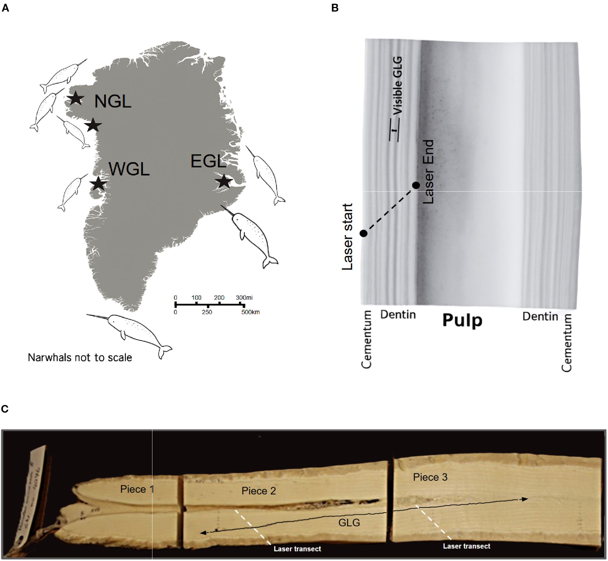
Figure 1. (A) Map of Greenland. Locations where whales were captured are highlighted with black stars. (B) Example of a narwhal tusk piece analyzed with LA-ICP-MS. Tusk piece showing a laser transect (black arrow) used to measure local element concentrations. The narwhal tusk has three main parts: the outer cementum (porous and flexible), the dentin (wherein groups of growth layers—GLGs—are visible), and the pulp cavity (which contains blood vessels and nerves; note that the pulp has been rinsed in this picture). (C) A tusk sectioned into smaller pieces. Since growth layers (black line) can stretch over several pieces, we need to consider the possibility of temporal overlap when running LA-ICP-MS over the laser transects (red dashed line). GLG delineation and laser transect paths are schematic representations for illustrative purposes only. In particular, the traced growth layer might not be accurately identified.

2 Materials and methods

2.1 Data acquisition and LA-ICP-MS

2.1.1 Sample collection, preparation, and analytical setup

The narwhal tusks were collected from Inuit hunts conducted between 2008 and 2018 (Table 1, Figure 1B). The tusks were previously sectioned longitudinally for prior studies, and age estimates for the tusks were obtained by counting GLGs (this study; Garde et al., 2012, 2024). For this study, the tusks were further cut into smaller pieces, each less than 10 cm in length, to fit the analytical equipment (Figure 1B). From these tusk pieces, we selected a subset where we took care to ensure that each piece contained unique growth layers not represented in previously selected pieces. This approach was designed to avoid temporal overlap in the signals obtained from the subsequent laser ablation analysis (Figure 1C). Calcium (Ca) was adopted as the internal standard element for these phosphate-rich tusk structures. We used X-ray fluorescence spectrometry (XRF) to quantify Ca content across the tusk growth layers, estimating an average concentration of 53.789 wt%.

Table 1

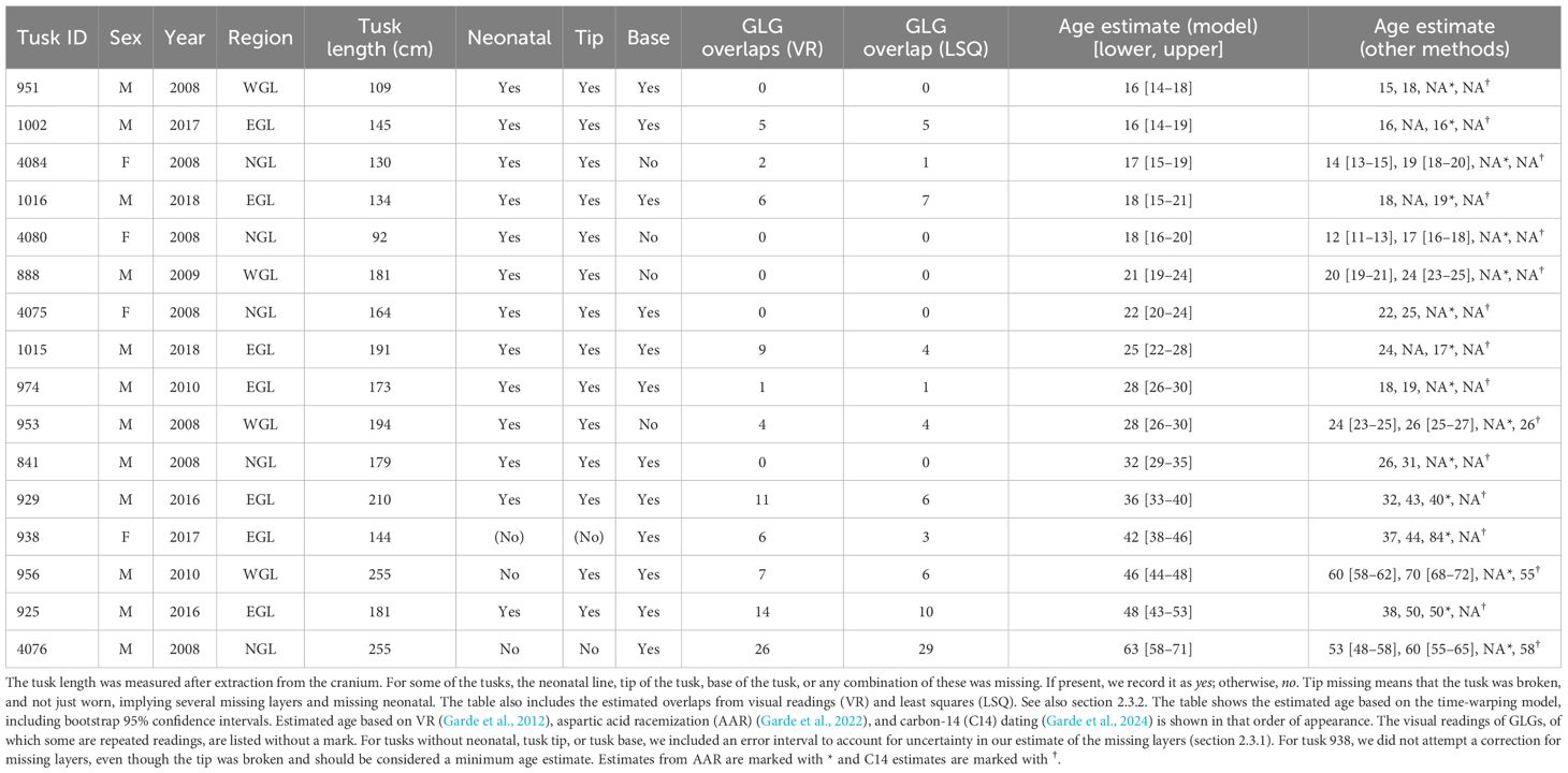
Table 1. Tusk samples used in this study and information about sex (F, female; M, male), and the year and region where the narwhal was captured (NGL, North Greenland; WGL, West Greenland, and EGL, East Greenland).

2.1.2 Microchemical analysis

The trace element composition of the narwhal tusk was measured along a transect running across the growth zones, from the cementum to the pulp cavity (Figure 1A), corresponding to the temporal progression of growth. The analyses were performed at the LA-ICP-MS facility at the Geological Survey of Denmark and Greenland (GEUS). An NWR213 frequency-quintupled Nd: YAG solid-state laser system from ESL, employing two-volume cell technology, was coupled to an ELEMENT2 double-focusing single-collector magnetic sector-field ICP-MS from Thermo Fisher Scientific. The operating conditions and data acquisition parameters are listed in Supplementary Table S1. The general analytical approach and data processing techniques used are described in Serre et al. (2018); Fink-Jensen et al. (2022, 2021), and Stounberg et al. (2022) with further details differing from these procedures given herein.

Laser counts per second were mapped to µg/g using Ca as internal calibrant (fixed at 53.789 wt% from our XRF average) and NIST-610 glass as reference material (see the Supplementary Materials). Drift was mitigated by flanking each transect with NIST-610 and BHVO-2 reference runs, and accuracy was checked against NIST-610/614 (2σ < 5% for >1 µg/g; see Supplementary Figure S1). Analyses were performed at 40 µm spot/10 Hz (2–3 J cm⁻²), with 30 s gas blank measurement and washout prior to each new run. Data reduction used the Trace Elements scheme in iolite4 (Hellstrom et al., 2008). In this paper, we focused on the resulting trace element signals relative to the major element Ca.

For full instrument models, optimization routines, oxide-ratio minimization, calibration curves, and XRF mapping workflow, see Supplementary Methods.

2.1.3 Omitting data from cementum and pulp cavity

The GLGs in the dentin are composed of alternating dark and light bands, which are believed to represent annual cycles, as confirmed in several species (Perrin et al., 2009; Scheffer and Myrick, 1980; Hohn et al., 2016; Waugh et al., 2018), such as belugas (Delphinapterus leucas) and harbor seals (Phoca vitulina). Dentin GLGs are preferred for age estimation because they are more easily distinguishable than cementum (Garde et al., 2012), and we follow this established practice. To isolate the part of the LA-ICP-MS signals corresponding to dentin, we measured the width of the cementum and pulp along the laser transect using a vernier caliper. Based on the laser’s movement speed of approximately 3 µm per second, we then truncated the signal at the corresponding time points. Because the junctions between dentin and cementum are not always clearly visible (Ho et al., 2004), we supplemented the caliper measurements by examining zinc (Zn) elemental signals in each tusk piece (Figure 2A), as Zn concentrations are known to be elevated in the cementum (Dean et al., 2018; Martin et al., 2007; Clark et al., 2020b). Additional evidence of elevated Zn concentrations was obtained by XRF spectroscopy (Figure 2B). We also observed a small increase in Zn at the end of the signal, where the laser enters the pulp chamber. This is likely because the Ca content in the pulp drops faster than the Zn content; thus, the Ca-normalized zinc levels spike. For pieces where this increase is clear, we also chose to trim the end of the signal to exclude the influence of pulp.

Figure 2

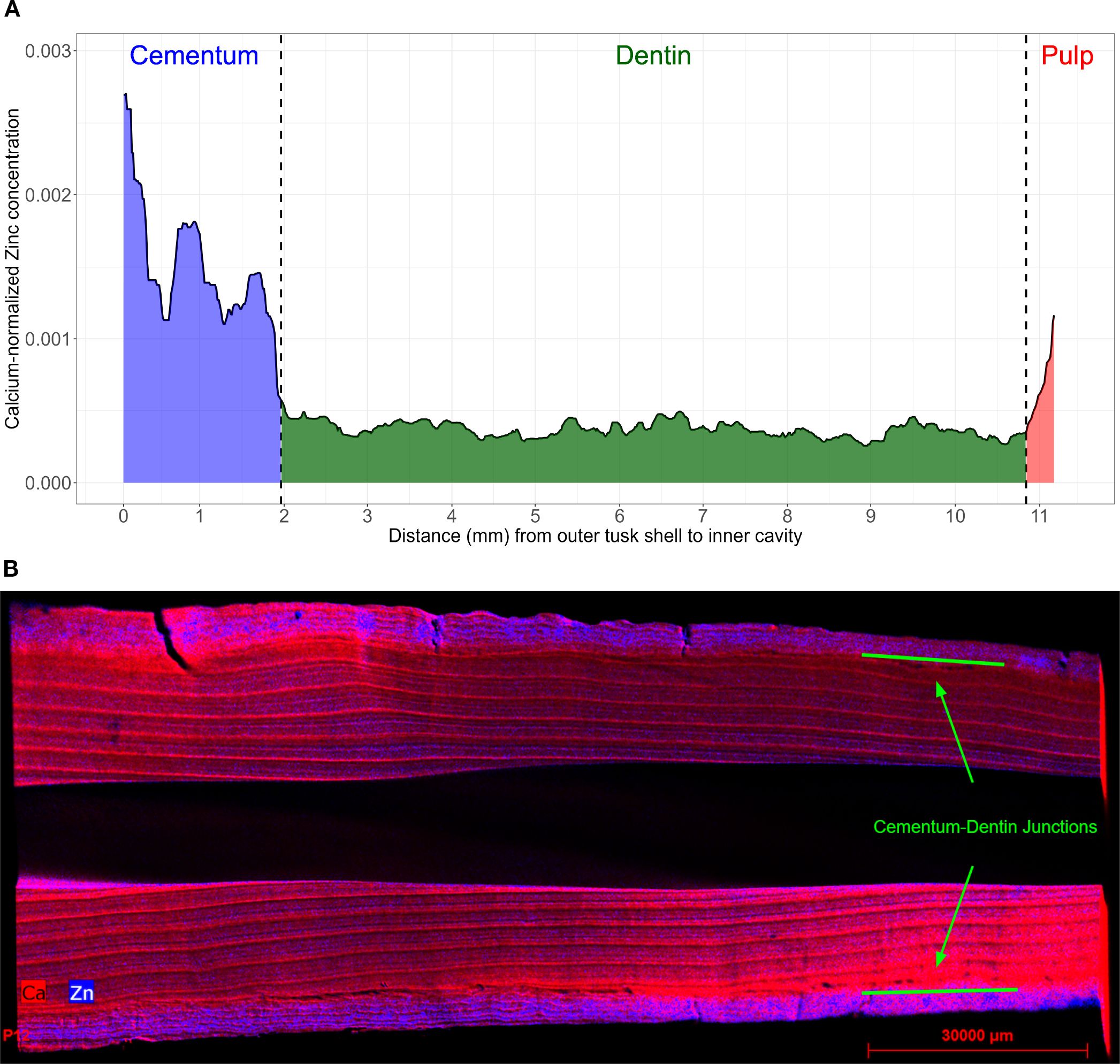
Figure 2. Zinc concentrations in tusk pieces. (A) LA-ICP-MS-derived zinc (the isotope ⁶⁶Zn) signal for tusk 956, piece V. The blue, green, and red areas are the presumed regions of cementum, dentin, and pulp, respectively. Regions of pulp and cementum show elevated zinc levels. (B) X-ray fluorescence tusk image. Zinc concentrations (in blue) in the cementum zone of a tusk piece, compared to the calcium levels (in red), mostly concentrated in the dentin zone.

2.2 Element signal decomposition and analysis

LA-ICP-MS generated signals for 15 elements (Supplementary Table S1) for each tusk piece across all 16 tusks. Here, we focused on Sr and Ba, since these elements are assumed to reflect seasonal migrations between winter and summer grounds through cyclic variations (Ruiz-Sagalés et al., 2024; Heimbrand et al., 2020), thereby providing proxy markers for age estimation. For the purpose of age estimation, trends add unnecessary complexity, as our model only needs to capture the dynamics of the repeating cycles. We therefore decomposed each signal into a trend component and a cyclic component, with focus on the latter. The trend components were estimated using local polynomial regression [locally estimated scatterplot smoothing (LOESS)] implemented in the statistical program R. This estimation was performed on the full tusk signal, by combining the signals from each tusk piece in chronological order. The cyclic components were then obtained by subtracting the estimated trend from the original signal (Figure 3). We chose the Spearman correlation coefficient to account for non-linear associations. Our proposed model assumes that the observed signals consist of a mean structure, expressed as a sum of sinusoidal functions, plus measurement error (Equation 1). The measurement error (noise) is explicitly modeled as normally distributed. Further details are provided in section 2.3. To reduce the variance of the noise term in the signals used for age estimation, we considered the average of Ba and Sr. We also assumed that all growth layers were present in the tusk piece, such that when pieces are gathered, the signal covers the entire lifespan of the narwhals (except for possible few missing layers; see section 4).

Figure 3

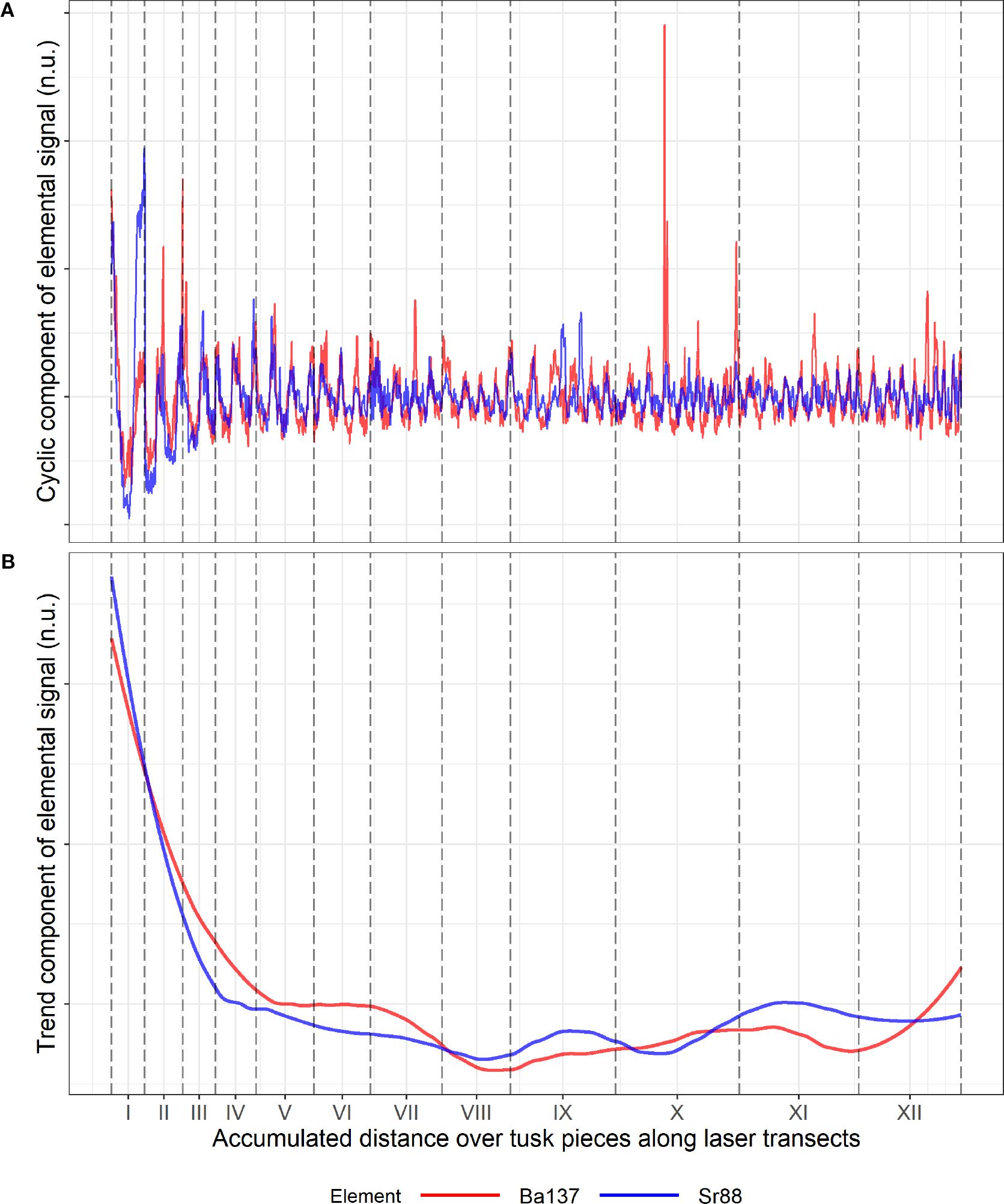
Figure 3. Standardized (no units; n.u.) signals of Ba (red) and Sr (blue), separated into a cyclic component (A) and a trend component (B) for 12 tusk pieces from tusk 956. Standardization was done by dividing each observation with the standard deviation of the signal. The trend was then obtained using local polynomial regression, with a span parameter equal to 30% of neighboring points. Vertical dashed lines mark transitions between tusk pieces. For this specific tusk, the Spearman correlation between Ba and Sr is 0.6 and 0.71 for the cyclic and trend component, respectively.

2.3 A time-warping model

In this section, we introduce the time-warping model fitted to the average Ba–Sr signals, which display cyclic patterns reflecting narwhal migratory behavior. These cycles alternate between larger and smaller peaks due to seasonal differences. We account for this by modeling the average dynamics as a sum of sinusoidal components, or “waves”, where the dominant wave models the overall annual dynamics and the second wave corrects for any shift in concentration between seasons. Because tusk growth rate vary over time, e.g., due to poor feeding year or illness, the rates are modeled stochastically, leading to a more realistic representation of the signal dynamics.

Let y_i = y(x_i) be the detrended (see section 2.2) element concentration of the average signal over Ba and Sr at a distance x_i = Δi from the cementum–dentin junction along the laser transect of the tusk piece, where Δ = x_i − x_i−1 is the distance between measurements for i = 1,…,n, with n equal to the number of measurements. The measurement at position x_i then corresponds to the element deposition at an unknown time through an increasing function g, t_i = g(x_i), which we denote the growth process, since the increase in g from position x_i to position x_i+1 gives the time passed for the tusk to grow a distance x_i+1 − x_i along the laser transect. We impose that g is a strictly increasing function with respect to x, which ensures that time never goes backward.

The growth process is defined as the integral of an instantaneous frequency process ξ_x [frequency at time t_x = g(x)], which we assume is stochastic due to environmental, seasonal, and internal variability in the growth rate of the tusk. The process ξ_x should be positive, since the tusk can only grow and not shrink. We assume that it varies stochastically around some mean growth rate α > 0. We use the so-called square root (SQR) diffusion, which is a positive stochastic process with governing equation.

$$d{\xi }_x=-\beta ({\xi }_x-\alpha )dx+\omega \sqrt{{\xi }_x}d{W}_x, {\xi }_0=0,$$

with parameters mean α, rate of adjustment $\beta$, and variance ${\omega }^2/2\beta$, and $W_t$ is a Wiener process modeling the unknown deviations from the mean as stochastic.

The growth process is then defined as $g(x)={\int }_0^x{\xi }_{s}ds$, so $g$ is also stochastic, and strictly increasing, since ${\xi }_x>0$, ensuring non-reversion of time. Whenever ${\xi }_x$ increases, it indicates a deceleration in the growth of the tusk (since the resulting increase in $g$ indicates that more time has passed for the same amount of dentinal growth).

We assume the following form for the progression of the element measurements:

$\begin{array}{ll}\begin{array}{c}{y}_i=\underset{\text{Annual cycles}}{\underbrace{A\text{sin}(g(x_i)+b)}}-\underset{\text{Summer}/\text{winter differences}}{\underbrace{B\text{cos}(2g(x_i)+2b)}}+{ϵ}_i, i\hfill \\ =0,1,\dots ,n;x_i=i\text{Δ};g(0)=0\hfill \end{array}& (1)\end{array}$

where ${ϵ}_i$ is assumed to be an independent and normally distributed measurement error with mean 0 and variance ${\sigma }^2,$, which could describe instrumental fluctuations, surface contamination, or small-scale variations not captured by the model mean. The parameter $A$ represents the baseline amplitude of the element concentration at the time of year of maximum concentration (summer or winter), while $B<A$ modulates this amplitude, accounting for seasonal variations. The offset parameter $b$ determines the point in the season of the birth of the animal.

The growth process $g(x)$ provides the current age in years at any spatial position $x_i$, through counting the elapsed number of cycles, such that:

$\begin{array}{ll}\text{Age}(x_i)=\text{Elapsed number of cycles}=\frac{g(x_i)}{2\pi },i=1,\dots ,n& (2)\end{array}$

$\begin{array}{ll}\text{Age of whale}=\text{Age}(x_n),& (3)\end{array}$

where $g(x)$ is the growth process of the entire tusk, and $x_n$ is the total distance covered across all tusk pieces. The model was fitted to each individual piece of the tusk, whereafter the growth processes were concatenated in chronological order, i.e., from the tip of the tusk to the root segment, taking into account possible overlaps (see section 4.3.2).

We then perform time warping, by expressing the observations y_i in terms of time coordinates t_i instead of length coordinates $x_i$.

The model was fitted using a variant of the Stochastic Approximation Expectation Maximization (SAEM) algorithm (Ditlevsen and Samson, 2014; Reiter et al., 2025). Residual bootstrapping was used to produce confidence intervals for the age estimate. It was performed on the fitted signal for each tusk piece to generate M = 100 bootstrapped versions of the growth process $g(x)$. A single bootstrapped version was randomly selected for each tusk piece, and the selected processes were then concatenated to form a complete growth process for the entire tusk. This procedure was repeated 100,000 times, generating 100,000 complete growth processes for each tusk, hence 100,000 age estimates using Equation 3. The empirical density of the bootstrapped estimates, with a small correction introduced in section 2.3.1, is then used for uncertainty quantification. See Reiter et al. (2025) and section 4.3 for details and further discussion of the model and the estimation method.

2.3.1 Missing layers

For tusk 956, the tip was worn and the neonatal line, along with a few layers, was likely missing. For tusk 4076, the tip was broken, and the neonatal line, along with several layers, was clearly missing. We incorporated this extra variability into our bootstrap procedure by uniformly sampling the number of missing layers from the intervals [0, 4] for tusk 956 and [5, 15] for tusk 4076. The chosen intervals were conservatively defined based on estimates from Garde et al. (2012). The study concluded that tusk 956 was missing only a few layers, if any, since the tip was present, but worn. In contrast, the tip of tusk 4076 was broken and this tusk was then compared to tusk 956, which shared similar physical characteristics from which a point estimate of 10 was made (Garde et al., 2012). An additional four tusks (888, 953, 4080, and 4084) were missing an estimated 5–7 cm at the base, based on physical comparison with intact tusks (Garde et al., 2012). The authors judged that the missing centimeters would correspond to only a few growth layers. For these tusks, we therefore sampled uniformly from the interval [0, 2]. This correction was consistently applied to both the bootstrap procedure and the visual readings. For instance, tusk 4076’s visual reading of 50 years, when adjusted for missing layers sampled from [5, 15], yielded a final estimate of 60 ± 5 years.

2.3.2 Overlapping pieces

Following the segmentation of a tusk into multiple pieces, particular attention was given to ensure that selected pieces used in this study covered all GLGs. Still, as previously stated, visually tracing GLGs is challenging (Figure 1C) and a conservative strategy was adopted, where we labeled any layer that was not clearly continuous with adjacent layers as a new GLG. This strategy minimizes the risk of undercounting GLGs, but can produce overlaps between adjacent pieces. To visually assess the exact amount of overlap, we re-traced the layers over consecutive tusk pieces (Figure 1C) under reflective light. This provided estimates that ranged from 0 to 14, with a median of four overlaps.

We used this visual assessment as the basis for a more objective, data-driven quantification of the extent of overlap, following the rules below. If the manual estimate of overlaps between two consecutive tusk pieces was zero, we accepted it without further analysis. If overlaps were identified, we calculated the sum of squares to determine the most likely overlap between consecutive tusk pieces, guided by the model estimated growth process $\widehat{g}(x)$, and the estimated phase $\widehat{b}$, from each tusk piece. The procedure can be summarized in four steps:

1. Identification of annual intervals. For each tusk piece, we used $\widehat{g}(x)$ and $\widehat{b}$ to identify the annual intervals, i.e., when a year starts and end, using Equation 4. This amounts to finding all x where $\widehat{g}(x)$ + $\widehat{b}$ is equal to an odd multiple of $\frac{\text{π}}{2}$.

2. Matching and comparing observations between consecutive tusk pieces. We aligned the observations y_i from each annual interval of the first tusk piece with the observations of the first annual interval of the adjacent tusk piece. This was done on the time-warped scale, i.e., by expressing observations in terms of time, y_i = y(t_i), such that measurements on one tusk piece were matched to measurements on the other tusk piece believed to be deposited at the same time. Because the spatial width of a GLG corresponding to one whole year (one cycle) varies, so too will the number of measurements from LA-ICP-MS. Following time warping, the years will be aligned in time, but will still contain a different number of measurements, resulting in different temporal resolutions. To ensure compatibility, we adjusted the resolution of the intervals of the first tusk piece, through interpolation or subsampling, to match the resolution of the annual interval of the second tusk piece. We standardized the observations to account for variations in scale. This was done by subtracting the signal mean and dividing by the signal standard deviation. Finally, we computed the average of the squared differences between observations from each interval of the first tusk piece and observations from the first interval of the second tusk piece.

3. Including unfinished year. Each tusk piece also had an unfinished year at the end of the signal. This interval (start of year to end of signal) was also included, and handled similarly as in step 2, except that it was compared to the same annual fraction of the interval from the following tusk piece.

4. Selecting the best match. We chose the interval from the first tusk piece, which had the smallest average difference, with the first interval of the second tusk piece, as our best estimate of an overlapping year. The overlapping data, along with remaining data beyond the boundary of that interval, were subsequently removed from the first tusk piece.

If only one annual peak was found in the first tusk piece, we then assumed that there was no overlap. Similarly, if the second tusk piece had just one peak, we also assumed no overlap. The entire procedure is visualized in Figure 4.

Figure 4

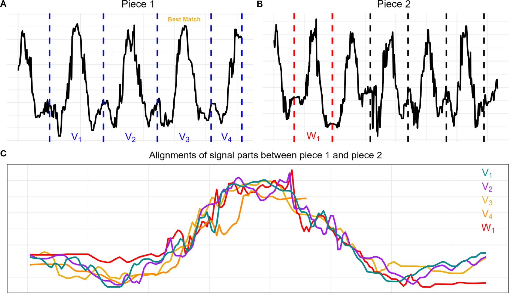
Figure 4. Illustration of the least-squares estimation for overlapping growth layers on tusk 956, between tusk pieces VIII and IX. (A) Time-warped signal of piece VIII. The signal traverses 3 years (V₁, V₂, and V₃), and we extend with an unfinished year V₄. (B) Time-warped signal of piece IX with the first year (W₁) marked by red dashed lines, and other years (unused) indicated by black horizontal lines. (C) The signal restricted to each present year (V₁, V₂, V₃, and V₄ shown in cyan, purple, yellow, and orange, respectively) in piece VIII is compared to the signal restricted to the first year of piece IX (W₁ shown in red). The best overlap (in the least-squares sense) occurs between V₃ and W₁. Each signal has been standardized prior to comparison. The method estimates an overlap of 1.57 years, compared to a visual reading of 1 year.

3 Results

We analyzed 16 narwhal tusks, each sectioned into multiple tusk pieces. We selected a subset of these pieces for each tusk (ranging from 6 to 16 pieces) expected to cover all GLGs, and used LA-ICP-MS on each piece to obtain 15 element signals.

3.1 Ba and Sr show strong seasonal cyclicity

Analysis of the 15 elements from LA-ICP-MS revealed that strontium (Sr) and barium (Ba) exhibited the most distinct cyclic variations (Figure 3). In addition, we found that Sr and Ba, among all elements, were most similar in terms of both their cyclic variations and their trend over time. For these two elements, the Spearman correlation test across pooled tusks showed a highly significant relationship (p < 10⁻⁴; Bonferroni-adjusted p-value for double testing), with an average (over all tusks) correlation pair of 0.49 and 0.57 for the trend and cycle component, respectively, higher among any other elements (Table 2). In addition to these cyclic variations, visible in elements such as Sr, lead (Pb), Ba, and lithium (Li), we observed that incorporation varied between groups of elements. For some elements, we observed a gradual decline in concentrations from early GLGs (near the tip; juvenile phase) to late GLGs (near the root; prime phase). Other elements showed more irregular patterns. For instance, Ba tended to be relatively high during the juvenile stage of a narwhal’s life, possibly due to dietary intake related to nursing (Clark et al., 2020a). Figure 3 also illustrates that the standardized Ba and Sr signals are almost interchangeable. While Ba and Sr may seem nearly identical, the signal-to-noise ratio can differ significantly within a tusk piece. We often noticed that the signal-to-noise ratio of Ba appeared inversely related to that of Sr. We refer to the Supplementary Materials for a 2-dimensional visualization of the (trend,cycle)–element correlation pairs.

Table 2

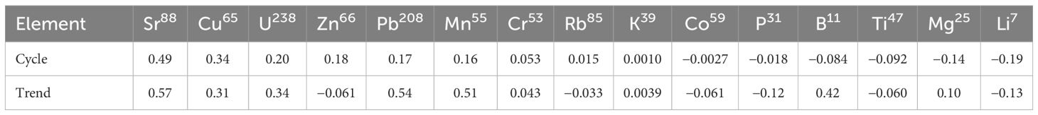
Table 2. Spearman correlation coefficients between Ba¹³⁷ and other trace elements for cyclic and trend components.

3.2 Age estimates and method comparison

The signal average of barium and strontium correlated with seasonal cycles, enabling the translation of spatial locations on tusk cross-sections into temporal events and providing age estimates through a novel time-warping model. The model captures both the deterministic seasonal component and stochastic deviations. In the example piece shown, the fitted signal closely follows the observed Ba–Sr oscillations (Figure 5A). Periods of higher (lower)-frequency fluctuations (Figure 5B) coincide with periods where the growth process g(x) is steep (flat) (Figure 5C), corresponding to local compression (expansion) of GLGs, which, in turn, means less (more) growth. For this tusk piece, when we integrate up all the frequency contributions, we see that growth process actually steepens, corresponding to declining growth. This is seen as increasingly contracted annual intervals, which, on the time-warped scale, were adjusted such that all annual intervals achieved equal length (Figure 5D). Table 1 provides complete information for all tusks, including our model’s age estimates and estimates from visual GLG counts, C14 dating, and AAR, as well as overlap detection assessments. Tusk 938 was broken, but we were not able to provide an informed interval for the missing Layers (Garde and Heide-Jørgensen, 2022); thus measurements (except for AAR) are to be considered minimum estimates. Overall, visual GLG readings and model estimates were consistent, except for tusks 956 and 974, where discrepancies persisted even when accounting for model uncertainty. AAR measurements for tusks 938 and 1015 also diverged from both model ages and visual readings, whereas the other four AAR values showed no substantial differences. Among the tusks, tusk 956, which records one model estimate, two visual readings, and a single C14 date, exhibited the greatest variability in age estimates across methods. In contrast, the C14 dates for tusks 953 and 4076 closely aligned with the other methods. Concerning overlaps, the visual readings and the least-squares estimation generally agreed, with some clear deviations for tusks 1015, 929 and 938 where the visual readings detected roughly twice as many overlaps. For several tusks, we saw sharp and narrow densities indicating high model confidence in age estimates (Figure 6). For tusks 4076, 925, 938, 929, and 841, we saw broader, flatter distributions reflecting greater uncertainty. The tusks were arranged from top to bottom by estimated mean age (Table 1, Figure 6), and illustrations were added to simultaneously visualize how age and length co-varied (Figure 6). The age–length relationship revealed a general positive trend, with older narwhals typically possessing longer tusks, though considerable variability was observed. Some older individuals exhibited relatively short tusks, while certain younger whales displayed disproportionately large ones, indicating that factors beyond age influence tusk size (Graham et al., 2020).

Figure 5

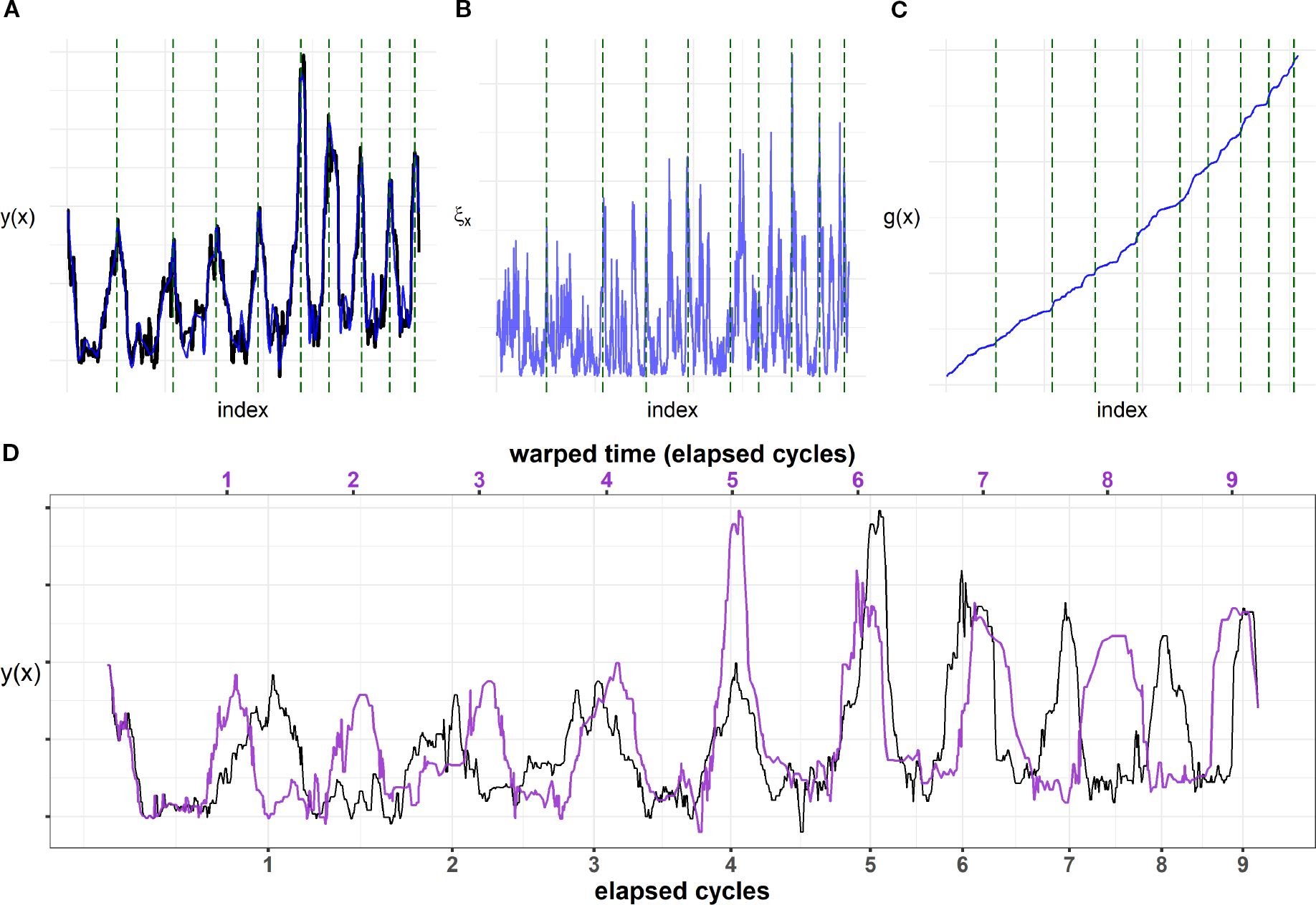
Figure 5. Model fit for tusk piece XII of tusk 956. (A) Raw signal (black) and fitted signal (blue). (B) Predicted square root process ξ_x (blue). (C) Growth process (blue). In all plots, estimated years (Equation 2) are marked as dashed green lines. (D) Time-warped signal (purple) and the original signal (black). Years are shown both on the time-warped scale (equidistant, upper axis) and on the original scale (lower axis). The time-warped signal is obtained by contracting longer periods (slow growth) and stretching shorter periods (rapid growth) such that all cycles have the same period.

Figure 6

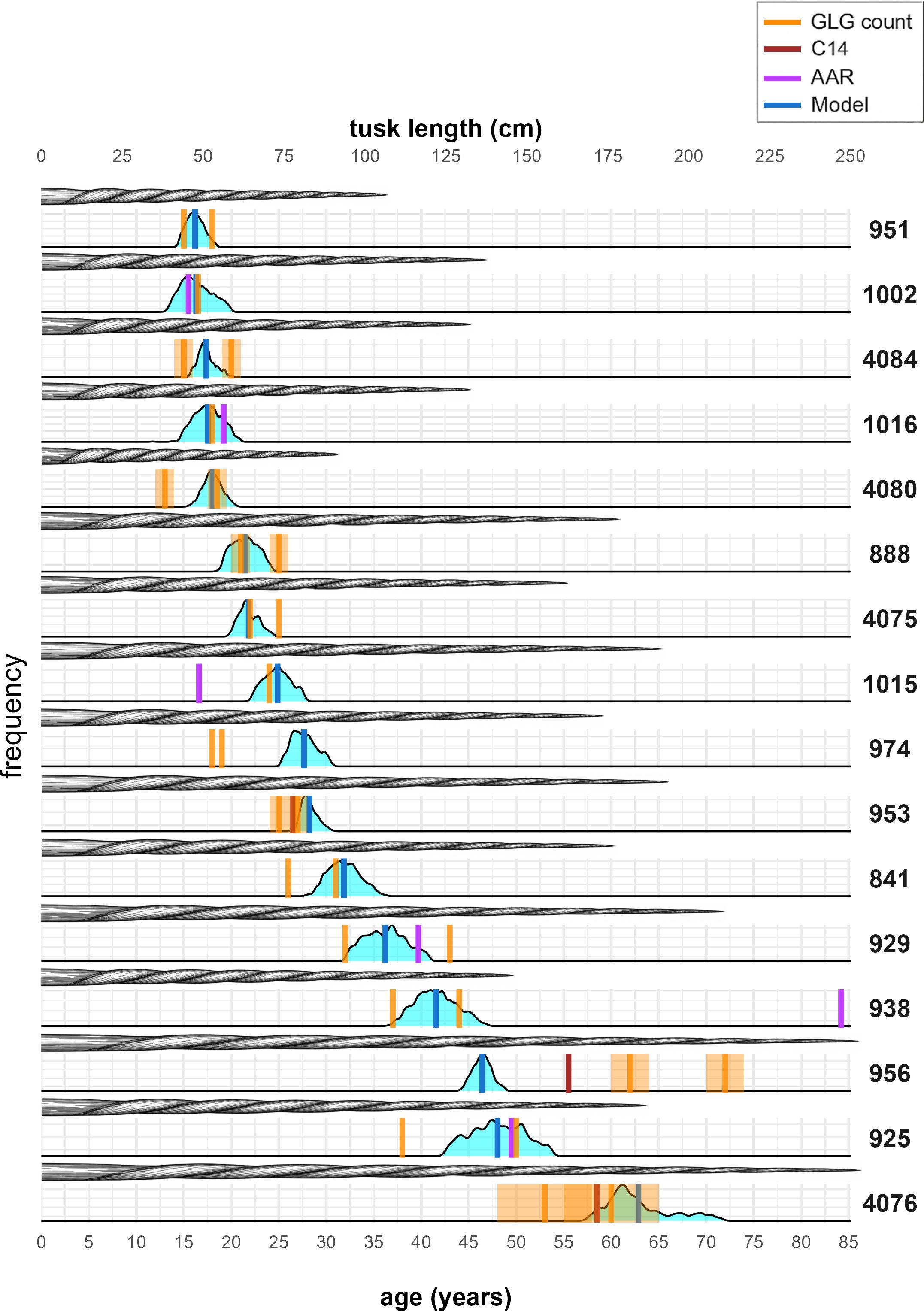
Figure 6. Age estimates and tusk lengths for the 16 tusks. Estimates from the time-warping model (section 2.3) are shown as dark blue vertical lines. Densities of residual bootstrap estimates are shown in light blue. The manual GLG readings of each tusk is shown as orange vertical lines (one to two readings for each tusk), along with light orange error bands from missing GLGs. Age estimates from AAR and C14 dating are shown in purple and brown, respectively. The lengths of the tusks are visualized with an illustration of each tusk and a corresponding length scale at the top. Tusks 974 and 956 show large (average) differences of 9 and 14 between model estimate and visual reading. Tusk 938 was broken at the tip; thus, both model estimates and visual readings are treated as minimum age estimates, which partially explain the large gap to AAR.

4 Discussion

4.1 Methods of age estimation

The traditional method for estimating the age of marine mammals is through counting of growth layers in the dentin or cementum of the teeth (Read et al., 2018; Scheffer and Myrick, 1980). However, visual reading is often difficult due to poor contrast between layers and the process of GLG counting is somewhat subjective with considerable variability in counts both within the same reader and between different readers, especially when assessing older individuals (Bowen et al., 1983; Lonati et al., 2019). Age estimation also relies on the assumption that one GLG is deposited each year (Stewart et al., 2006)—an assumption that, while generally accepted, has stirred some debate (Brodie et al., 2013). Finally, factors like attrition of the erupted tusk (seen mainly in older individuals) can wear away the neonatal line that marks the onset of the GLG deposition—this was seen in tusks 4076 and 956 (see Table 1). For the embedded tooth, dentinal occlusion can obscure the visibility of GLGs (Watt et al., 2020; Read et al., 2018). This last point is why GLG counting is in many cases considered a minimum age estimate (Read et al., 2018). Despite these limitations, visual readings remain popular because it provides a cost-effective method that can be applied to large samples without demanding expensive laboratory analyses, unlike techniques based on AAR, C14 (Stewart et al., 2006; Garde et al., 2012), or even LA-ICP-MS. On the other hand, specialized analyses eliminate inter-observer variability and subjective interpretation inherent in visual readings, while providing age estimates where GLG reading fails due to poor preservation or tooth wear. The higher accuracy and reproducibility of these biochemical methods justifies their cost when reliable age estimation is essential.

4.2 Segmentation, signal quality, and biological artifacts

Our proposed method for age estimation needs only a rough identification of GLGs, in order to properly segment the tusk and identify pieces covering new sets of GLGs, used for the subsequent LA-ICP-MS analysis. Still, this segmentation procedure risks either counting certain GLGs several times across consequent tusk pieces or failing to identify intermediate layers (although the latter is considered unlikely). If not corrected for, this can then skew the age estimate towards higher values. In this study, we have attempted to address this last point by estimating the number of overlapping GLGs, under the assumption that the collection of tusk pieces cover all GLGs with possible repetitions between adjacent pieces. We have done this using a least-squares approach between time-warped signals of consecutive tusk pieces. This admittedly involves unaccounted uncertainty that increases with each new comparison. For the purpose of age estimation, an alternative strategy would be to incorporate the uncertainty relating to overlaps in the bootstrap procedure, similar to what we did with missing layers. We chose the least-squares alignment approach because it provides a logical, objective means of merging tusk piece signals into a single, continuous timeline that has use-cases beyond age estimation. The problem of repeated GLGs across pieces is specific to this dataset of narwhal tusks, where tusks need to be sectioned to fit the LA-ICP-MS equipment, a constraint not typically encountered with smaller, more compact specimens. To overcome this issue for future large specimens, segmentation should ideally produce spatially contiguous (gap-free) pieces capable of fitting the LA-ICP-MS equipment.

Concerning the analyzed LA-ICP-MS signals, we found that this collection was quite diverse. Some signals showed clear cyclicity whereas others displayed elevated noise levels slightly obscuring such repeated patterns. This directly influenced estimate precision. Tusks with clear, repeating cycles (Figure 3A) conforming to the model specified by Equation 1 yielded narrow uncertainty bands. Signals with irregular patterns, including secondary cycles (see the next paragraph), produced bootstrap replicates with greater variability and correspondingly wider confidence intervals (Figure 6; Supplementary Figure S3). This is because we resample residuals in the bootstrap procedure. If residuals are skewed or not conforming to the normal assumption (for whatever reason), the resulting bootstrapped signals can create new spurious cycles or eliminate existing ones.

Another subtlety is the existence of sub-annual layers (or accessory layers), likely associated with life-history events such as periods of low food consumption (Read et al., 2018; Zhao et al., 2025). Accessory layers are sporadically embedded within the primary growth layers and risk being misidentified as GLGs when doing visual readings, which is likely an important cause for the high variability seen in GLG counting. It is hypothesized that such sub-annual layers could potentially manifest as secondary cycles in the element signals used in this study, thereby adding further variability to the final age estimate. These secondary cycles may appear as embedded peaks within annual peaks (Figure 5; note the additional peak in the third elapsed cycle, which may be due to accessory layers). Small embedded peaks were seen in several barium and strontium signals, but with a size negligible to the major peaks associated with the primary growth layers. These embedded peaks also carry over to the cyclic part of our signal, when we perform the decomposition described in section 2.2. For tusk 938, base occlusion potentially obscured several layers. This, together with the missing layers not accounted for, could explain the gap between AAR and the other methods. Overlap detection differences between methods contributed to some age discrepancies. Algorithmic overlap estimates closely matched visual assessments for tusks 4084, 951, 888, and 4075 (difference ≤ year). For tusk 1015, the difference between model age estimate and closest visual reading was 4 years when correcting for overlap, reducing to 1 year when overlaps were included. We consider these issues to be ubiquitous in relation to GLG-based age estimation, underscoring the intrinsic challenges posed by biological complexity and environmental influences rather than methodological shortcomings.

4.3 Classifying seasonal peaks

We obtain age estimates by fitting the time-warping model introduced in the preprint (Reiter et al., 2025) to cyclic element signals. The model is specified in Equation 1 and assumes that the signals contain two distinct annual peaks of varying magnitude due to seasonal differences. For the narwhal tusks, this pattern is believed to be due to migration between summer and winter grounds, where the composition of prey items and, hence, mineral intake likely differs. The assumption may not hold true for every single annual cycle, which may introduce error in the age estimate. For example, if two consecutive peaks were winter peaks, but were modeled as a winter and a summer peak due to level differences, the model would interpret growth as proceeding more slowly, and using Equation 2, we would count one elapsed year when in fact it was two. When signals exhibit negligible seasonal variation such that B ≈ 0 in Equation 1, two scenarios may arise. In the first scenario, summer and winter peaks are roughly equal in magnitude, and this will surely lead to overestimation of the number of cycles using our model. In the second scenario, one of the seasonal peaks shows negligible magnitude relative to the other. The determination between these scenarios depends on the nature of the signals and the ecological context. For narwhals, whose feeding ecology suggests one dominant seasonal peak, the condition B ≈ 0 would indicate the second scenario. It is worth noting that, although we observed a pattern of alternating high and low peaks in our studied population, this may not be a common feature across other narwhal populations.

4.4 Beyond narwhal age estimation

Our extensive dataset of trace elements provides insights that go beyond simple age estimation. The time-warping framework introduced in section 2.3 effectively translates spatial locations on the tusk to an annual timeline, which allows us to compare changes in trace elements within the tusk to environmental conditions in specific years or periods. For instance, uranium or lead concentrations could be examined in relation to records of Arctic pollution. Biological processes can also be inferred from selected trace elements, such as barium or strontium, where abrupt shifts early in life may indicate the timing of weaning (Clark et al., 2020a). Finally, a few elements (magnesium, potassium, and rubidium) lacked a clear seasonal pattern, but instead showed consistent high concentrations in the central dentin across tusk pieces, which likely reflect underlying biological processes.

Beyond narwhals, our model can be applied to other species with teeth or tusks that form growth layers, as well as to other mineralized tissues and other growth structures with annual cyclic patterns in selected elements. Examples include elephant and walrus tusks, beluga or mammoth teeth, and even fish otoliths. This assumes that a tracer can be identified that reliably reflects annual cycles and conforms to the model specified by Equation 1. If there are no seasonal differences, one can remove the second sinusoidal term by setting B = 0 in the model equation.

Overall, this demonstrates the usefulness of our method, not only for age estimation across species, but also for translating spatial measurements of annual deposited element records into an annual timeline, opening the door to further ecological and physiological analyses.

Data availability statement

The original contributions presented in the study are included in the article/Supplementary Material. Further inquiries can be directed to the corresponding author.

Ethics statement

Ethical approval was not required for the study involving animals in accordance with the local legislation and institutional requirements because Tusk specimens was obtained from local narwhal hunts in Greenland, and Greenland Institute of Natural Resources have permission to purchase these. Importation of specimens into Denmark was authorized by CITES permits IM 0721-199/08, IM 0721-200/08, IM 0905-590/17, IM 0822-296/18, IM 1115-726/16 and DK-2021-0067486-01.

Author contributions

LR: Methodology, Software, Formal Analysis, Visualization, Writing – original draft, Conceptualization. TT: Investigation, Writing – review & editing, Data curation. BH: Investigation, Data curation, Writing – review & editing. AS: Methodology, Supervision, Writing – review & editing. DW: Resources, Methodology, Writing – review & editing, Investigation. MH-J: Data curation, Supervision, Conceptualization, Writing – review & editing, Methodology, Investigation. SD: Writing – review & editing, Methodology, Supervision, Funding acquisition, Conceptualization, Project administration. EG: Conceptualization, Writing – review & editing, Supervision, Methodology, Data curation, Investigation.

Funding

The author(s) declare financial support was received for the research and/or publication of this article. This work was supported by NordForsk (grant number 105053) and the French–Danish CNRS International Research Network MaDeF IRN. SD was funded by the Novo Nordisk Foundation (grant no. NNF20OC0062958). The micro-xrf work at the Natural History Museum of Denmark was funded by grant 7408 from the Villum Foundation to Michael Storey. The funders NordForsk, Novo Nordisk Foundation, Villum Foundation and the French–Danish CNRS International Research Network MaDeF IRN were not involved in the study design, collection, analysis, interpretation of data, the writing of this article or the decision to submit it for publication.

Acknowledgments

We thank Christina Lockyer for two visual GLG readings of tusks 925 and 929 (counts 50 and 43, respectively). We would also like to thank the two reviewers for their highly valuable feedback.

Conflict of interest

The authors declare that the research was conducted in the absence of any commercial or financial relationships that could be construed as a potential conflict of interest.

Generative AI statement

The author(s) declare that Generative AI was used in the creation of this manuscript. Figures 1A and B have been edited and enhanced using OpenAI’s ChatGPT (model GPT-3.5). The tusk animation used in Figure 6 is entirely generated by GPT-3.5.

Any alternative text (alt text) provided alongside figures in this article has been generated by Frontiers with the support of artificial intelligence and reasonable efforts have been made to ensure accuracy, including review by the authors wherever possible. If you identify any issues, please contact us.

Publisher’s note

All claims expressed in this article are solely those of the authors and do not necessarily represent those of their affiliated organizations, or those of the publisher, the editors and the reviewers. Any product that may be evaluated in this article, or claim that may be made by its manufacturer, is not guaranteed or endorsed by the publisher.

Supplementary material

The Supplementary Material for this article can be found online at: https://www.frontiersin.org/articles/10.3389/fmars.2025.1655427/full#supplementary-material

References

Binda G., Di Iorio A., and Monticelli D. (2021). The what, how, why, and when of dendrochemistry:(paleo) environmental information from the chemical analysis of tree rings. Sci Total Environ. 758, 143672. doi: 10.1016/j.scitotenv.2020.143672, PMID: 33277003

PubMed Abstract | Crossref Full Text | Google Scholar

Bowen W., Sergeant D. E., and Øritsland T. (1983). Validation of age estimation in the harp seal, phoca groenlandica, using dentinal annuli. Can. J. Fisheries Aquat. Sci. 40, 1430–1441. doi: 10.1139/f83-165

Crossref Full Text | Google Scholar

Brodie P., Ramirez K., and Haulena M. (2013). Growth and maturity of belugas (delphinapterus leucas) in cumberland sound, Canada, and in captivity: evidence for two growth layer groups (glgs) per year in teeth. J. Cetacean Res. Manage. 13, 1–18. doi: 10.47536/jcrm.v13i1.550

Crossref Full Text | Google Scholar

Clark C. T., Horstmann L., and Misarti N. (2020a). Evaluating tooth strontium and barium as indicators of weaning age in pacific walruses. Methods Ecol. Evol. 11, 1626–1638. doi: 10.1111/2041-210X.13482, PMID: 33381293

PubMed Abstract | Crossref Full Text | Google Scholar

Clark C. T., Horstmann L., and Misarti N. (2020b). Zinc concentrations in teeth of female walruses reflect the onset of reproductive maturity. Conserv. Physiol. 8, coaa029. doi: 10.1093/conphys/coaa029, PMID: 32308984

PubMed Abstract | Crossref Full Text | Google Scholar

Council, N. R., on Earth, D., Board, O. S., and on Potential Impacts of Ambient Noise in the Ocean on Marine Mammals, C (2003). Ocean noise and marine mammals. doi: 10.17226/10564, PMID: 25057640

PubMed Abstract | Crossref Full Text | Google Scholar

Dean C., Le Cabec A., Spiers K., Zhang Y., and Garrevoet J. (2018). Incremental distribution of strontium and zinc in great ape and fossil hominin cementum using synchrotron x-ray fluorescence mapping. J. R. Soc. Interface 15, 20170626. doi: 10.1098/rsif.2017.0626, PMID: 29321271

PubMed Abstract | Crossref Full Text | Google Scholar

Dietz R., Desforges J.-P., Rigét F. F., Aubail A., Garde E., Ambus P., et al. (2021). Analysis of narwhal tusks reveals lifelong feeding ecology and mercury exposure. Curr. Biol. 31, 2012–2019. doi: 10.1016/j.cub.2021.02.018, PMID: 33705717

PubMed Abstract | Crossref Full Text | Google Scholar

Ditlevsen S. and Samson A. (2014). Estimation in the partially observed stochastic Morris–Lecar neuronal model with particle filter and stochastic approximation methods. Ann. Appl. Stat 8, 674–702. doi: 10.1214/14-AOAS729

Crossref Full Text | Google Scholar

Fink-Jensen P., Hüssy K., Thomsen T. B., Serre S. H., Søndergaard J., and Jansen T. (2022). Lifetime residency of capelin (mallotus villosus) in west Greenland revealed by temporal patterns in otolith microchemistry. Fisheries Res. 247, 106172. doi: 10.1016/j.fishres.2021.106172

Crossref Full Text | Google Scholar

Fink-Jensen P., Jansen T., Thomsen T. B., Serre S. H., and Hüssy K. (2021). Marine chemistry variation along Greenland’s coastline indicated by chemical fingerprints in capelin (mallotus villosus) otoliths. Fisheries Res. 236, 105839. doi: 10.1016/j.fishres.2020.105839

Crossref Full Text | Google Scholar

Garde E., Ditlevsen S., Olsen J., and Heide-Jørgensen M. P. (2024). A radiocarbon bomb pulse model for estimating the age of North Atlantic cetaceans. Biol. Lett. 20, 20240350. doi: 10.1098/rsbl.2024.0350, PMID: 39592001

PubMed Abstract | Crossref Full Text | Google Scholar

Garde E. and Heide-Jørgensen M. P. (2022). Tusk anomalies in narwhals (Monodon monoceros) from Greenland. Polar Res. 41. doi: 10.33265/polar.v41.8343

Crossref Full Text | Google Scholar

Garde E., Peter Heide-Jørgensen M., Ditlevsen S., and Hansen S. H. (2012). Aspartic acid racemization rate in narwhal (Monodon monoceros) eye lens nuclei estimated by counting of growth layers in tusks. Polar Res. 31, 15865. doi: 10.3402/polar.v31i0.15865

Crossref Full Text | Google Scholar

Garde E., Tervo O. M., Sinding M.-H. S., Nielsen N. H., Cornett C., and Heide-Jørgensen M. P. (2022). Biological parameters in a declining population of narwhals (Monodon monoceros) in Scoresby Sound, Southeast Greenland. Arctic Sci 8, 329–348. doi: 10.1139/as-2021-0009

Crossref Full Text | Google Scholar

Graham Z. A., Garde E., Heide-Jørgensen M. P., and Palaoro A. V. (2020). The longer the better: evidence that narwhal tusks are sexually selected. Biol. Lett. 16, 20190950. doi: 10.1098/rsbl.2019.0950, PMID: 32183636

PubMed Abstract | Crossref Full Text | Google Scholar

Hay K. A. (1980). Age determination of the narwhal, monodon monoceros l. Rep. Int. Whaling Commission Special Issue 3, 119–132.

Google Scholar

Hay K. A. (1984). The life history of the narwhal, monodon monoceros l., in the eastern canadian arctic. Montreal, Quebec, Canada: McGill University.

Google Scholar

Heide-Jørgensen M. P., Dietz R., Laidre K. L., Richard P., Orr J., and Schmidt H. C. (2003). The migratory behaviour of narwhals (monodon monoceros). Can. J. Zoology 81, 1298–1305. doi: 10.1139/z03-117

Crossref Full Text | Google Scholar

Heimbrand Y., Limburg K. E., Hüssy K., Casini M., Sjöberg R., Palmén Bratt A.-M., et al. (2020). Seeking the true time: Exploring otolith chemistry as an age-determination tool. J. fish Biol. 97, 552–565. doi: 10.1111/jfb.14422, PMID: 32515105

PubMed Abstract | Crossref Full Text | Google Scholar

Hellstrom J., Paton C., Woodhead J., and Hergt J.. (2008). Iolite: software for spatially resolved la-(quad and mc) icpms analysis. Mineralogical Assoc. Canada short course Ser. 40, 343–348. doi: 10.3749/9780921294801.app09

Crossref Full Text | Google Scholar

Ho S., Balooch M., Goodis H., Marshall G., and Marshall S. (2004). Ultrastructure and nanomechanical properties of cementum dentin junction. J. Biomed. Materials Res. Part A: Off. J. Soc. Biomaterials Japanese Soc. Biomaterials Aust. Soc. Biomaterials Korean Soc. Biomaterials 68, 343–351. doi: 10.1002/jbm.a.20061, PMID: 14704976

PubMed Abstract | Crossref Full Text | Google Scholar

Hohn A. A., Lockyer C. H., and Acquarone M. (2016). Report of the workshop on age estimation in monodontids. NAMMCO 68. doi: 10.7557/3.3743

Crossref Full Text | Google Scholar

Kelvin M., Whiteman E., Petrus J., Leybourne M., and Nkuna V. (2022). Application of la-icp-ms to process mineralogy: Gallium and germanium recovery at kipushi copper-zinc deposit. Minerals Eng. 176, 107322. doi: 10.1016/j.mineng.2021.107322

Crossref Full Text | Google Scholar

Koch J. and Günther D. (2011). Review of the state-of-the-art of laser ablation inductively coupled plasma mass spectrometry. Appl. Spectrosc. 65, 155A–162A. doi: 10.1366/11-06255, PMID: 21513587

PubMed Abstract | Crossref Full Text | Google Scholar

Lonati G. L., Howell A. R., Hostetler J. A., Schueller P., De Wit M., Bassett B. L., et al. (2019). Accuracy, precision, and error in age estimation of florida manatees using growth layer groups in earbones. J. Mammalogy 100, 1350–1363. doi: 10.1093/jmammal/gyz079, PMID: 31379391

PubMed Abstract | Crossref Full Text | Google Scholar

Martin R. R., Naftel S. J., Nelson A. J., and Iii W. D. S. (2007). Comparison of the distributions of bromine, lead, and zinc in tooth and bone from an ancient Peruvian burial site by x-ray fluorescence. Can. J. Chem. 85, 831–836. doi: 10.1139/v07-100

Crossref Full Text | Google Scholar

Perrin W. F., Würsig B., and Thewissen J. G. M. (2009). Encyclopedia of marine mammals (San Diego: Academic Press).

Google Scholar

Read F., Hohn A., and Lockyer C. (2018). A review of age estimation methods in marine mammals with special reference to monodontids. NAMMCO Sci. Publications 10. doi: 10.7557/3.4474

Crossref Full Text | Google Scholar

Reiter L. N., Heide-Jørgensen M. P., Garde E., Samson A., and Ditlevsen S. (2025). A time warping model for seasonal data with application to age estimation from narwhal tusks.

Google Scholar

Ruiz-Sagalés M., García-Vernet R., Sanchez-Espigares J., Halldórsson S. D., Chosson V., Sigurðsson G. M., et al. (2024). Baleen stable isotopes reveal climate-driven behavioural shifts in north atlantic fin whales. Sci Total Environ. 955, 177164. doi: 10.1016/j.scitotenv.2024.177164, PMID: 39447890

PubMed Abstract | Crossref Full Text | Google Scholar

Scheffer V. B. and Myrick A. (1980). A review of studies to 1970 of growth layers in the teeth of marine mammals. Rep. Int. Whal. Commn 3, 51–63.

Google Scholar

Serre S. H., Nielsen K. E., Fink-Jensen P., Thomsen T. B., and Hüssy K. (2018). Analysis of cod otolith microchemistry by continuous line transects using la-icp-ms. GEUS Bull. 41, 91–94. doi: 10.34194/geusb.v41.4351

Crossref Full Text | Google Scholar

Smith T. M., Cook L., Dirks W., Green D. R., and Austin C. (2021). Teeth reveal juvenile diet, health and neurotoxicant exposure retrospectively: What biological rhythms and chemical records tell us. BioEssays 43, 2000298. doi: 10.1002/bies.202000298, PMID: 33721363

PubMed Abstract | Crossref Full Text | Google Scholar

Stewart R., Campana S., Jones C., and Stewart B. (2006). Bomb radiocarbon dating calibrates beluga (delphinapterus leucas) age estimates. Can. J. Zoology 84, 1840–1852. doi: 10.1139/z06-182

Crossref Full Text | Google Scholar

Stounberg J., Thomsen T. B., Heredia B. D., and Hüssy K. (2022). Eyes and ears: A comparative approach linking the chemical composition of cod otoliths and eye lenses. J. Fish Biol. 101, 985–995. doi: 10.1111/jfb.15159, PMID: 35817955

PubMed Abstract | Crossref Full Text | Google Scholar

Vighi M., Borrell A., Víkingsson G., Gunnlaugsson T., and Aguilar A. (2019). Strontium in fin whale baleen: A potential tracer of mysticete movements across the oceans? Sci Total Environ. 650, 1224–1230. doi: 10.1016/j.scitotenv.2018.09.103, PMID: 30308810

PubMed Abstract | Crossref Full Text | Google Scholar

Walther B. D. and Thorrold S. R. (2006). Water, not food, contributes the majority of strontium and barium deposited in the otoliths of a marine fish. Mar. Ecol. Prog. Ser. 311, 125–130. doi: 10.3354/meps311125

Crossref Full Text | Google Scholar

Watt C., Heide-Jørgensen M., and Ferguson S. (2013). How adaptable are narwhal? a comparison of foraging patterns among the world’s three narwhal populations. Ecosphere 4, 1–15. doi: 10.1890/ES13-00137.1

Crossref Full Text | Google Scholar

Watt C. A., Stewart B. E., Loseto L., Halldorson T., and Ferguson S. H. (2020). Estimating narwhal (monodon monoceros) age using tooth layers and aspartic acid racemization of eye lens nuclei. Mar. Mammal Sci 36, 103–115. doi: 10.1111/mms.12623

Crossref Full Text | Google Scholar

Waugh D. A., Suydam R. S., Ortiz J. D., and Thewissen J. (2018). Validation of growth layer group (glg) depositional rate using daily incremental growth lines in the dentin of beluga (delphinapterus leucas (pallas 1776)) teeth. PloS One 13, e0190498. doi: 10.1371/journal.pone.0190498, PMID: 29338011

PubMed Abstract | Crossref Full Text | Google Scholar

Zhao S.-T., Matthews C. J., and Watt C. A. (2025). δ15n and δ13c cycles in narwhal (monodon monoceros) embedded teeth reveal seasonal variation in ecology and/or physiology. R. Soc. Open Sci 12, 242237. doi: 10.1098/rsos.242237, PMID: 40078917

PubMed Abstract | Crossref Full Text | Google Scholar