CoDeMap: a classification scheme for benthic habitats from the coast to the deep sea in the Mediterranean and Black Sea

The spatial representation of benthic habitats is essential across various applications, such as biodiversity monitoring, ecosystem management and conservation, and maritime spatial planning. In this context, classification schemes provide a universally understandable framework to characterize and chart the seafloor. This work introduces the Coast to Deep Mapping (CoDeMap) classification scheme for benthic habitats from the coast to the deep-sea environments. It consists of three main components (Morphology, Substrate and Biology) and it is conceived as a practical tool for users from various backgrounds who need to organize and interpret marine observational data, as well as characterize and map seafloors. While primarily developed for the Mediterranean Sea and the Black Sea, CoDeMap serves as a foundational framework that can be adapted to address any current or future similar request worldwide.

1 Introduction

The term “habitat” refers to the geographical, abiotic, and biotic characteristics of the environment where a species resides in any state of its life cycle. Habitat is an essential element of the seascape, frequently associated with diversity, functioning, and ecosystem services (Sokołowski et al., 2021). As a result, habitats became the primary classification unit in marine cartography and the focus of inventories, classification systems, and spatial mapping efforts (Coggan et al., 2007). In mapping, “habitat” is often used with a broader meaning and embraces more species, coming closer to the term “biotope”, i.e., the physical conditions in which a specific group of species lives (Montefalcone et al., 2021). Misiuk and Brown (2024) define benthic habitat mapping as “a spatially continuous prediction of biological patterns on the seafloor,” refining the earlier definition provided by Brown et al. (2011), which described it as “the use of spatially continuous environmental data sets to represent and predict biological patterns on the seafloor (whether continuous or discontinuous).”

The spatial representation of the distribution and extent of physically distinct areas of the seafloor, which are linked to groups of species or communities that consistently coexist (Harris and Baker, 2020), is vital for several reasons. In fact, maps on the distribution of benthic habitats facilitate to:

- identify biodiversity hotspots and provide inventories of vulnerable species and ecosystems, and critical or sensitive areas (Vassallo et al., 2018);

- orient conservation actions by identifying priority areas for protection (Angeletti et al., 2021; Ware and Downie, 2020) and plan effective management strategies (Fraschetti et al., 2011);

- consider a habitat-based approach in policy support and decision-making processes (Bianchi et al., 2012; Danovaro et al., 2020; Sokołowski et al., 2021);

- meet the requirements of European directives and programs (Schiele et al., 2014), such as the Habitat Directive (92/43/EEC), the Marine Strategy Framework Directive (2008/56/EC), the Biodiversity Strategy for 2030 (EU, 2020), the Nature Restoration Law (EU Regulation 2022/869);

- monitor anthropogenic impacts, environmental status and trends (Bekkby et al., 2020; Enrichetti et al., 2020; Gerovasileiou et al., 2019; Holon et al., 2015);

- assess seafloor economic resources and quantify ecosystem services (Cogan et al., 2009; McQuaid et al., 2020);

- implement modeling approaches to predict areas suitable for species and communities and detect changes (Azzola et al., 2021; Beca-Carretero et al., 2020; Bellin and Rossi, 2024; Martin et al., 2014; Moraitis et al., 2019; Vassallo et al., 2018).

The usage of benthic habitat classification systems is fundamental (Montefalcone et al., 2021) to characterize and describe the habitats (Robinson and Levings, 1995). In particular, a classification scheme provides a structured framework for the description and standardization of the physical and biological conditions defining habitat classes (Strong et al., 2019).

Numerous Benthic Habitat Classification Schemes (BHCSs) have been developed with different goals around the world (Table 1). Many of these schemes and lists are incompatible with each other, making it difficult to compare habitat types across studies and regions (Greene et al., 2008). Numerous scientific papers have reviewed existing classification systems for marine benthic habitats, discussed the revision process, and identified gaps (Diaz et al., 2004; Fraschetti et al., 2008; Galparsoro, 2012; Misiuk and Brown, 2024; Montefalcone et al., 2021; Strong et al., 2019).

Table 1

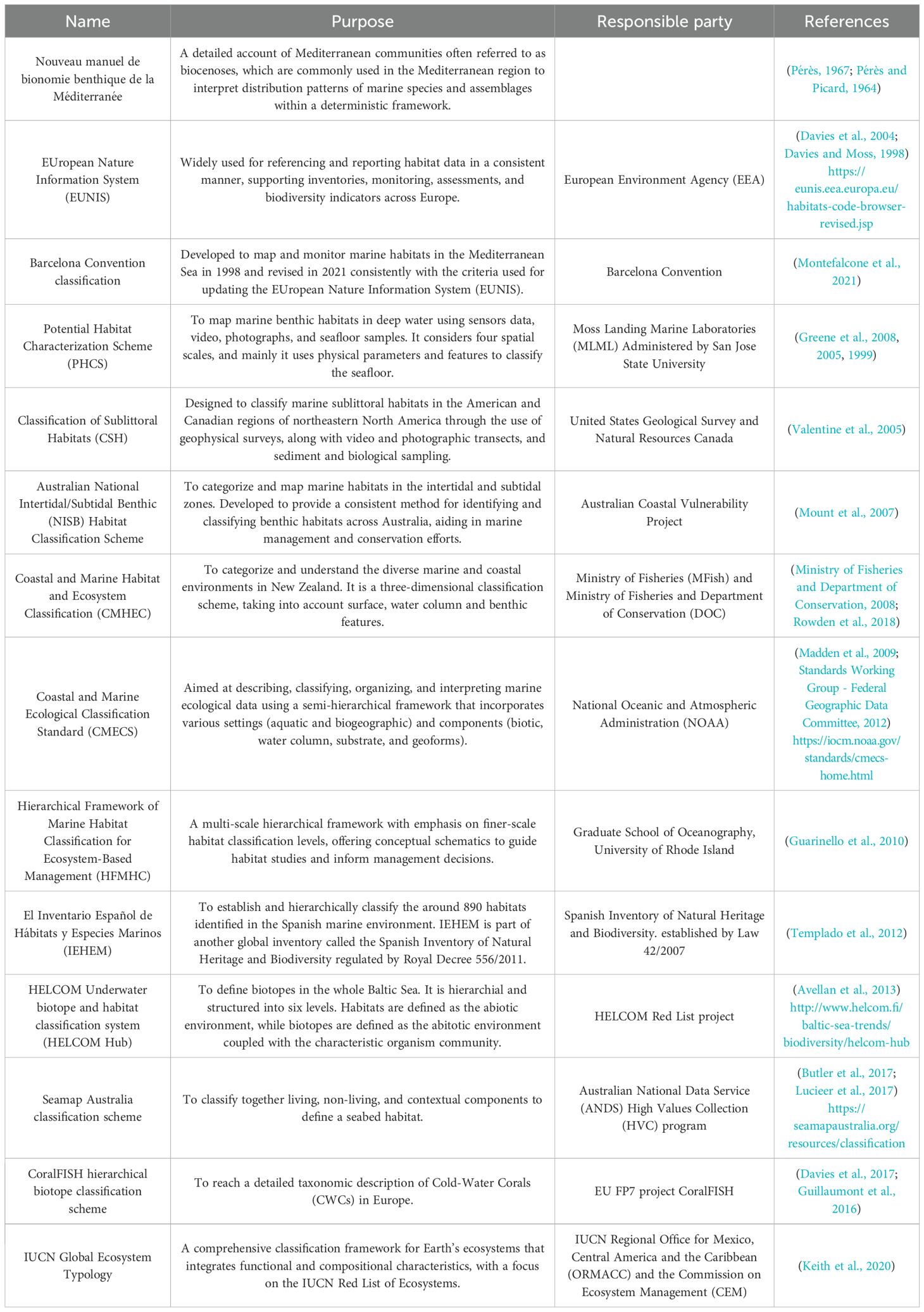
Table 1. Non-exhaustive list of international, European and regional classification schemes.

This paper introduces the Coast to Deep Mapping (CoDeMap) benthic habitats classification scheme (BHCS) for the Mediterranean and Black Sea benthic habitats from the coast to the deep sea. The philosophy behind CoDeMap is to provide a practical and operative tool for users from different backgrounds who need to organize and interpret marine observational data, as well as to describe, classify, and map seafloors.

2 CoDeMap benthic habitats classification scheme

CoDeMap BHCS is inspired by already existing classification schemes (EUNIS, CMECS, Seamap Australia) and habitats lists (IEHEM, Pérès and Picard (1964), Annex II of the Habitats Directive, Templado et al. (2012)) with a focus on the commonly underrepresented mesophotic and deep-sea environments. The aim during development of the CoDeMap was to create a classification scheme:

- Scientifically-based but easily applicable, with separated abiotic and biotic components defining the benthic habitat to minimize the uncertainties and biases introduced with the subjective interpretation;

- Hierarchical, its components are organized in subcomponents and sublevels able to catch the complexity of seafloor according to the availability and quality level of spatial data;

- Multiscale, user can capture the most relevant scale-dependent patterns and the high complexity and spatial heterogeneity of the seafloor, encompassing both abiotic and biotic characteristics;

- Multipurpose, CoDeMap is compatible with all mapping techniques. Users can map according to (i) typology, availability, and quality of the spatial data, (ii) the user expertise, (iii) the target (abiotic maps, single biota maps, community maps, benthoscape maps), and (iv) the purpose of the spatial representation (e.g. scientific papers, monitoring activities, inventory, prediction models, legislation background, habitat-based management measures);

- Flexible, CoDeMap is primarily designed for the Mediterranean and Black Sea, but it could be easily applied to any marine situation worldwide through the adaptations of its codes; the ability to combine classes allows for the description of habitat mosaics, enabling more accurate representation of seabed conditions that do not fit neatly into predefined classes;

- Dynamic and public, CoDeMap is publicly available (https://codemap.my.canva.site/about) including versioning and a form for the contribute implementing of the scheme. Indeed, it provides a baseline suitable to be constantly updated addressing increase of knowledge and predictable future changes of marine ecosystems.

2.1 Components, subcomponent, levels and classes

The CoDeMap scheme is organized into three main components: 1) Morphology, 2) Substrate, and 3) Biology (Figure 1).

Figure 1

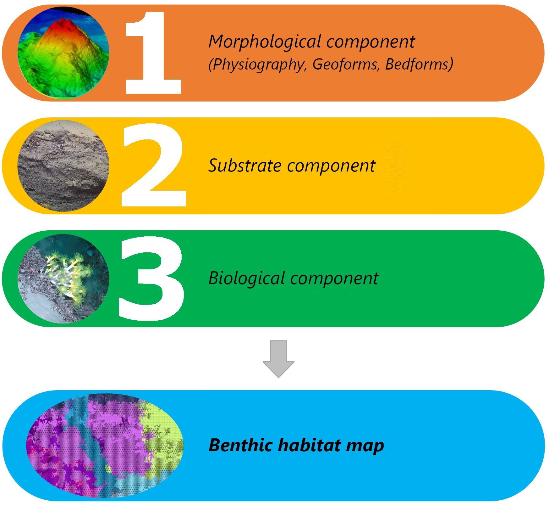
Figure 1. The three components of the CoDeMap benthic habitat classification scheme (Morphology, Substrate and Biology).

Internally, the main components are systemized hierarchically, with a series of subcomponents, levels, and classes (Figure 2). Seafloor morphology, type of substrate, and distribution of individual species or communities can be mapped separately and then merged into a single map of benthic habitats by using GIS software.

Figure 2

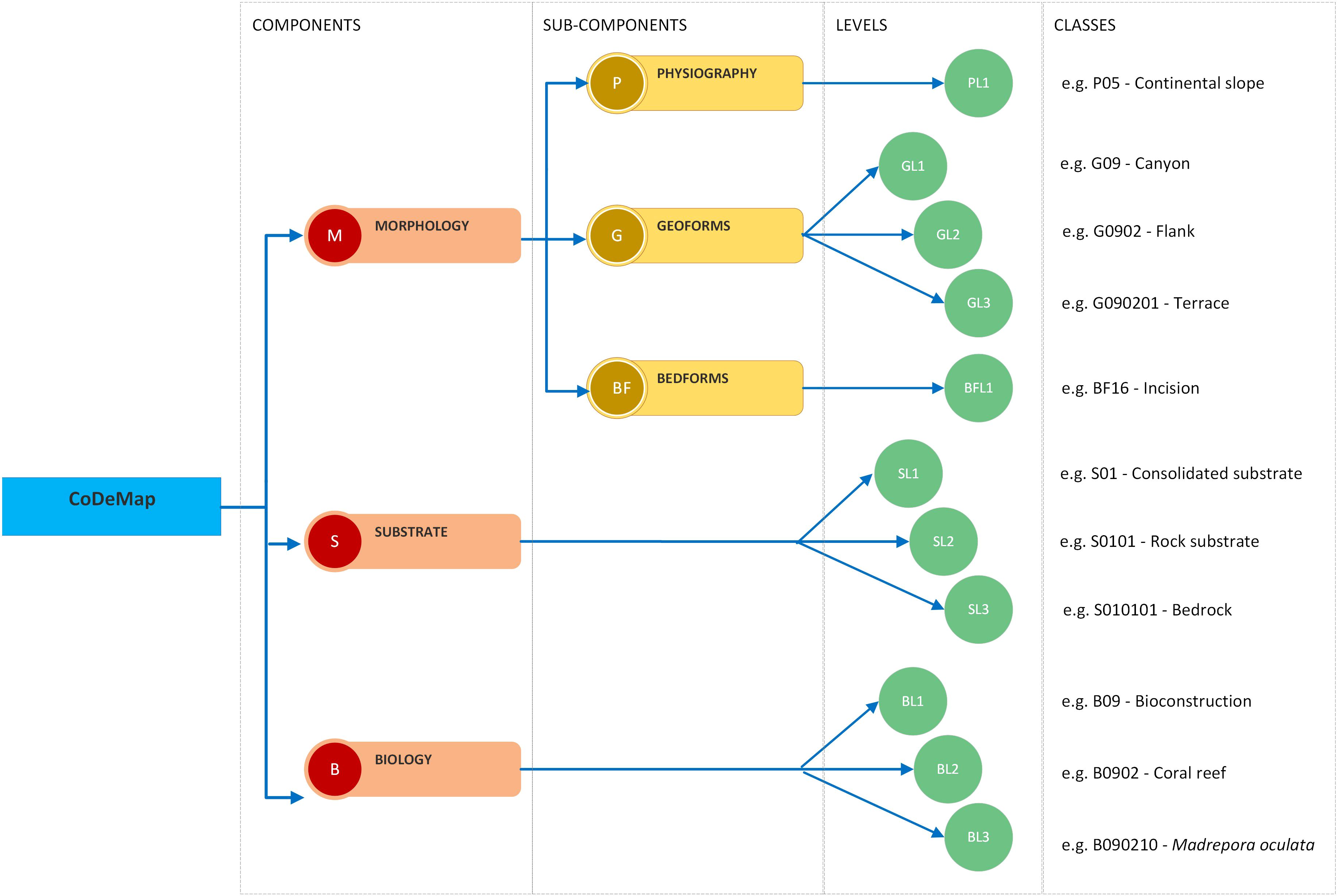
Figure 2. Structure of the CoDeMap BHCS showing the three components (red squares), the sub-components (yellow squares), and the levels (green circles). The levels contain the classes defined by a code and a label.

More specifically, the CoDeMap morphology components consist of subcomponents organized in descending order of size and level of detail 1) Physiography, 2) Geoforms, and 3) Bedforms. Within each subcomponent, levels are used to classify features from a broader scale (Level 1, L1) to small-scale features (L2, L3). In particular, the Physiography sub-component contains one level (PL1), while the Geoforms sub-component contains three levels (GL1, GL2, and GL3), and the Bedforms sub-component contains one level (BFL1). The Substrate and Biology components include three levels each, SL1, SL2, SL3 and BL1, BL2, BL3 respectively (Figure 2).

The sum of the three components (Morphology, Substrate and Biology) returns a benthic habitat map where each class is uniquely and unequivocally represented. The maximum number of levels describing a habitat class is 11, but not all levels must perforce contain information.

Each class of the scheme is identifiable by a univocal alphanumeric code and a label (Figure 2). Both the complexity of the code and the detail expressed with the label of the features increase from L1 to L3. Within L3 of substrate and biology, classes can be more specific (e.g. B020302 – Codium adherens) or more generic (e.g. B020301- Green algae) in bold in the scheme. To limit the proliferation and redundancy of classes in the scheme, codes can be combined to describe situations characterized by multiple classes, ordered by prevalence. The combination is permitted if more classes coexist and there is a representativeness of at least 25%. For example, an area characterized by coralligenous (spatial coverage=75%) and Posidonia oceanica (spatial coverage=25%) can be described as B0907+B040403. Conversely, a Posidonia oceanica meadow (coverage=75%) with interspersed coralligenous outcrops (coverage=25%) can be codified as B040403+B0907.

The legend can be customized to include only codes, only labels, or a combination of both. Additionally, users can select which levels to display according to the complexity and purpose of the representation (see paragraph 3).

2.1.1 Morphological component

Within the Morphology component, the Physiography sub-component includes only level PL1, which comprises the different constituents of the continental margin (i.e., moving from shallow to deep areas, coast, shelf, continental slope, basin plain, etc). The Geoform sub-component is divided into three levels (GL1, GL2, GL3). GL1 concerns environments and large-scale morphological features (e.g. beach, submarine canyon, leveed channels). GL2 refers to medium-scale morphologies and/or sub-environments (e.g. foreshore, canyon flank), while GL3 considers small-scale morphologies (e.g. shoreface bar, intra-canyon plunge pool, intra-lobe channel). For example, in the CoDeMap scheme a terrace on a canyon flank is coded G090201, (G09 - Canyon, G0902 - Flank, G090201 - Terrace). The Bedform sub-component consists of 17 features at a single level (encoded BF01, BF02, BF03, etc.). Therefore, a morphological feature can be described hierarchically using a complete code consisting of the union of sub-components. If along the continental slope (P05) a canyon (G09), whose flank (G0902) is marked by several incisions (BF16) the final code will result in: P02G0902BF16. In order to gather and organize all these classes together, we considered works like Ashley (1990); Dove et al. (2020); Harris et al. (2014), and Micallef et al. (2018).

2.1.2 Substrate component

The Substrate component classifies seabed nature and consists of three levels (SL1, SL2, SL3). SL1 distinguishes between consolidated (i.e. hard substrate), unconsolidated (i.e. soft substrate), and semi-consolidated substrate (i.e. various stages of lithification). SL2 provides information about the type of seabed (e.g. rocky substrate, firmground, biogenic unconsolidated substrate), similarly to the CMECS. SL3 considers the grain size (e.g. gravel, sand, mud) according to Wentworth (1922), and the type of sediment (e.g. cohesive mud, bioclastic sand, coral rubble). Therefore, an area characterized by blocks and boulders is coded as Consolidated substrate (S01), Rocky substrate (S0101), and Block and boulder (S010102).

2.1.3 Biological component

The Biology component consists of three levels (BL1, BL2, BL3). The coarsest level (BL1) considers different morpho-functional groups representing the seascape, (e.g., turf, forest, bioconstruction). BL2 specifies broad taxonomic groups represented in BL1. While, BL3 includes the highest possible taxonomic level, genus or species, (e.g., Callogorgia verticillata), or morpho-functional groups of species (e.g., red algae and massive sponges). BL3 has been conceived to allow experts and non-expert users to document more detailed biodiversity information. For example, the code B090737 indicates a Bioconstruction (B09) made by Coralligenous (B0907) characterized by Massive sponges (B090737).

Considering a mosaic of habitats characterized by the co-occurrence in high number of Madrepora oculata (B090210) and Poecillastra compressa (B070222) (coverage=60% and 40%, respectively), it should be categorized as “M. oculata” + “P. compressa” (B090210+B070222). If the user cannot (or is not able to) recognize a single species or several taxa typifying the area, it is also possible to mix different levels of the component. Following the previous example, a coral reef made by M. oculata (coverage=60%) + and a ground dominated by massive sponge where it is not possible to recognize the dominant species (coverage=40%) will be coded as B090210+B0702. The order of the two classes is related to their relative abundance. It is possible to reverse the codes if the coverage is different: B0702+B090210 identified an area characterized by a massive sponge ground (coverage=60%) and a coral reef built by M. oculata (coverage=40%).

The possibility to mix classes from different components permits the user to classify each item with a unique code in CoDeMap. Meaning what the Posidonia oceanica is identified by the code B040203, which can be associated with different substrate types (e.g. P. oceanica on sand is classified as S030301B040203 and P. oceanica on matte is classified as S030105B040203).

Several classification schemes and lists have been considered to compile the biological components, among others: EUNIS, IEHEM, Annex II of the Habitat Directive 92/43/EEC, Classification of benthic marine habitat types for the mediterranean region (SPA/RAC, 2006) and, IUCN Red List of Threatened Species.

3 GIS applications

This section describes four applications of the CoDeMap BHCS for different mapping scenarios, which are characterized by different scales, knowledge backgrounds and purposes. In the first application, the tool is used to create a large-scale map of benthic habitats for the Southern Adriatic (Mediterranean Sea) based on indirect and inhomogeneous geophysical data. The second example uses CoDeMap to describe the Tricase Canyon (Adriatic Sea), considering all three components of the scheme. The third application, CoDeMap is used to map the seafloor of the Dohrn Canyon (Tyrrhenian Sea) that has been surveyed by a Remotely Operated Vehicle (ROV). Finally, the fourth case study is a comparison between the CoDeMap and EUNIS classification schemes in the continental shelf along the Apulian coast (South Adriatic Sea).

3.1 South Adriatic continental margin

The South Adriatic Sea has been investigated by the CNR-ISMAR throughout the last 20 years by the acquisition of a large amount of geophysical data (multibeam and seismic), seabed samples (grab samples, box cores), and video from ROV. The interpretation of these data provided the basis to produce a geomorphological map of the South Adriatic continental margin (Campiani et al., 2024), and a benthic habitat map published in Prampolini et al. (2021). In this application, we have classified these two products using the CoDeMap BHCS producing several maps representing the morphology, the substrate, the biology, and the benthic habitat map of the basin.

Figure 3A represents the Morphology component classified according to the Physiography sub-component. In Figure 3B, the morphologic classification includes the level of Physiography (PL1) and the three levels of Geoforms (GL1, GL2, GL3), increasing the detail and the complexity of the seascape. The complete South Adriatic morphology is charted in Figure 4, where all the sub-components (Physiography, Geoforms and Bedforms) were used to build the map. These three representations of the South Adriatic morphology enhance the increase in scale, detail and complexity of the depicted seascape, by applying different levels of the CoDeMap BHCS and consequently, changing the information represented on the map.

Figure 3

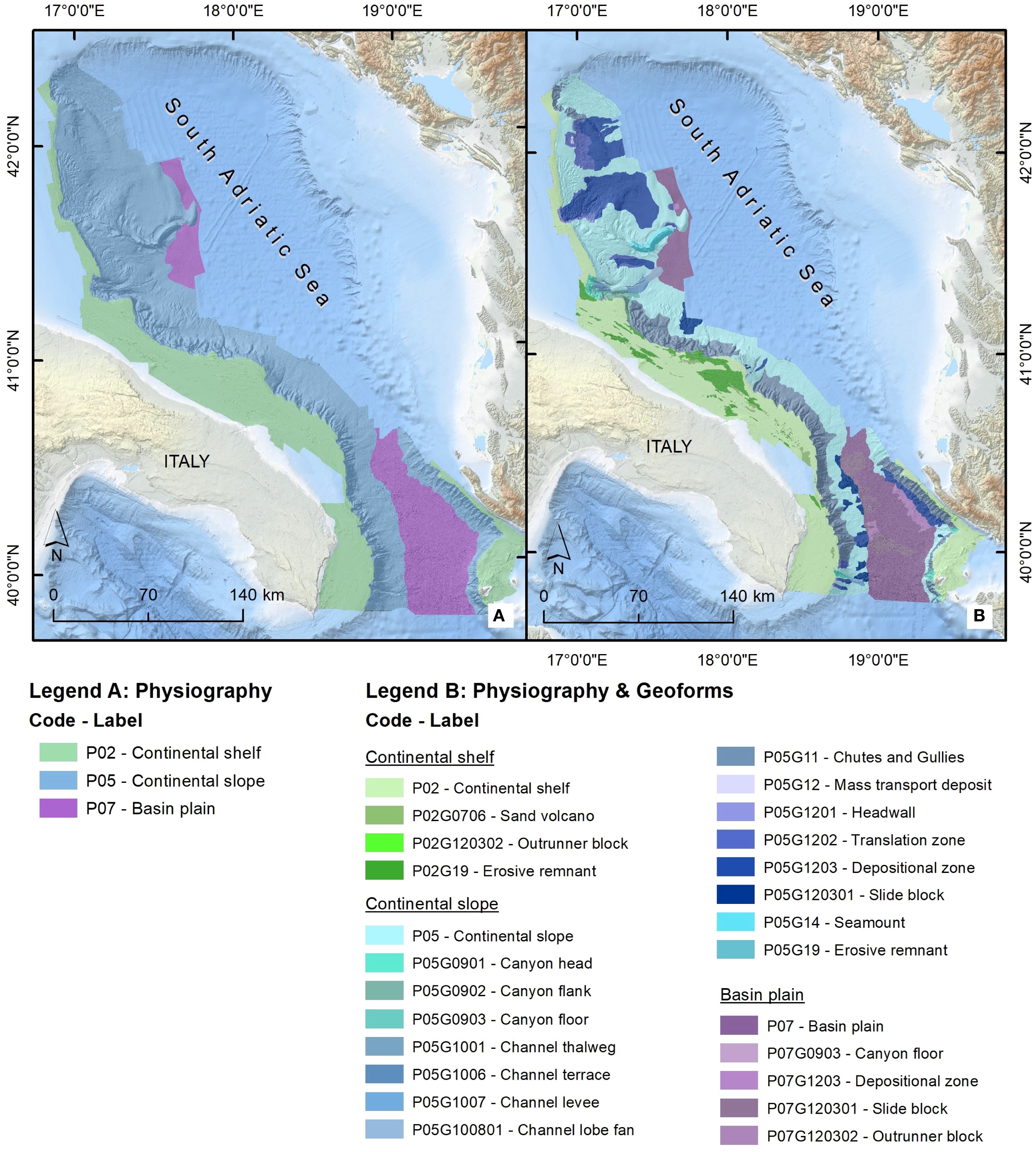
Figure 3. Morphology of the South Adriatic continental margin classified according to CoDeMap BHCS: (A) Physiography sub-component, (B) Physiography and Geoforms sub-components. Background: EMODnet Bathymetry World Base Layer version 1.

Figure 4

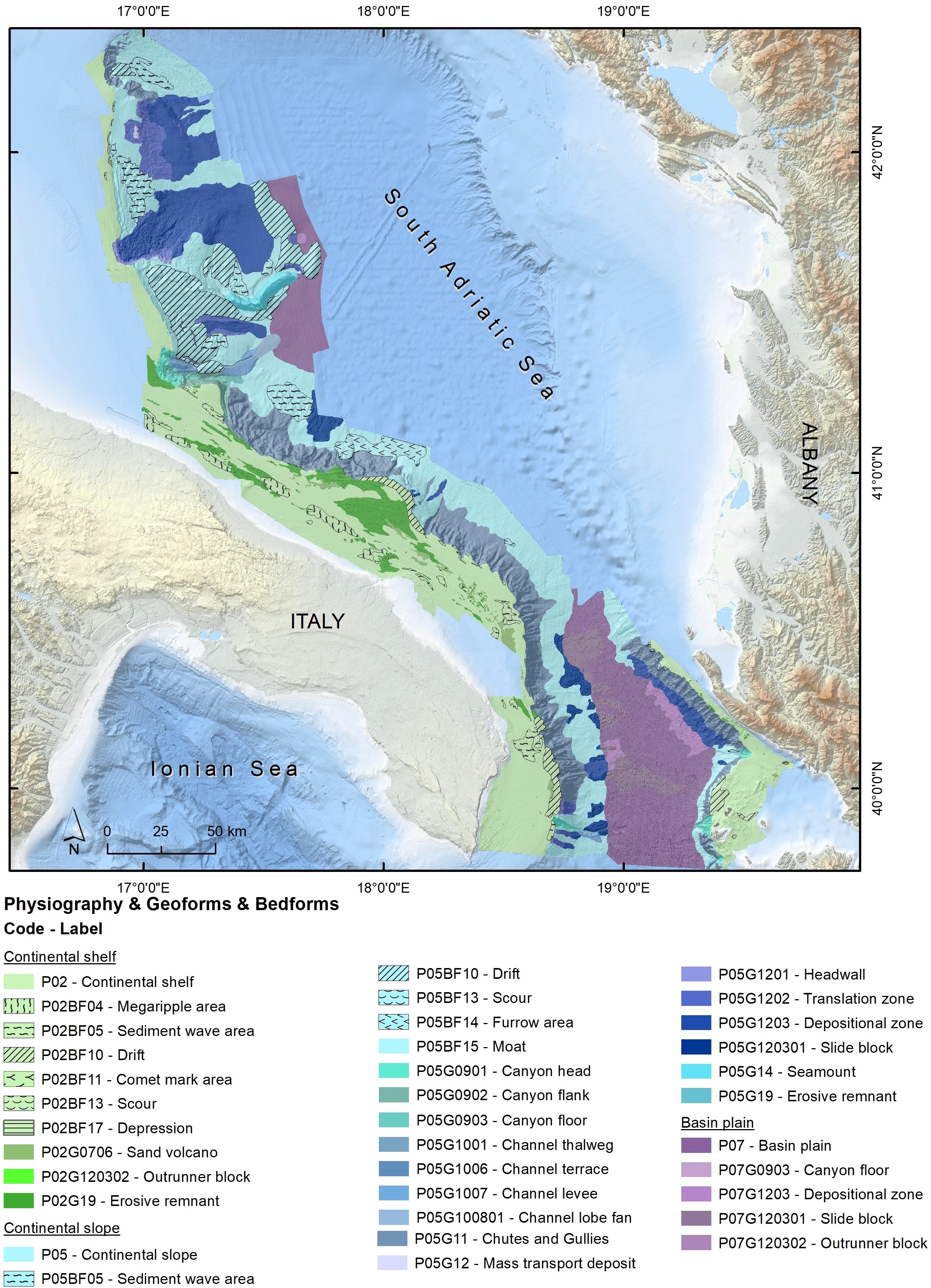
Figure 4. Morphology of the South Adriatic continental margin according to CoDeMap BHCS: full classification of the Morphology component using all the three sub-components: Physiography, Geoforms and Bedforms. For each element of the legend, the full code is shown coupled with the label of the most detailed class of the CoDeMap BHCS. Background: EMODnet Bathymetry World Base Layer version 1.

The South Adriatic continental margin has been classified according to information on substrate and biology at different levels of detail. The map in Figure 5 derives from the interpretation of seabed reflectivity and samples; the latter permitted to specify substrate texture and biological communities living on the seafloor. The substrate is described by all levels of the CoDeMap Substrate component and represented by using distinct colors range and tones according to the texture. The Biology component is depicted through a halftone screen superimposed on the substrate.

Figure 5

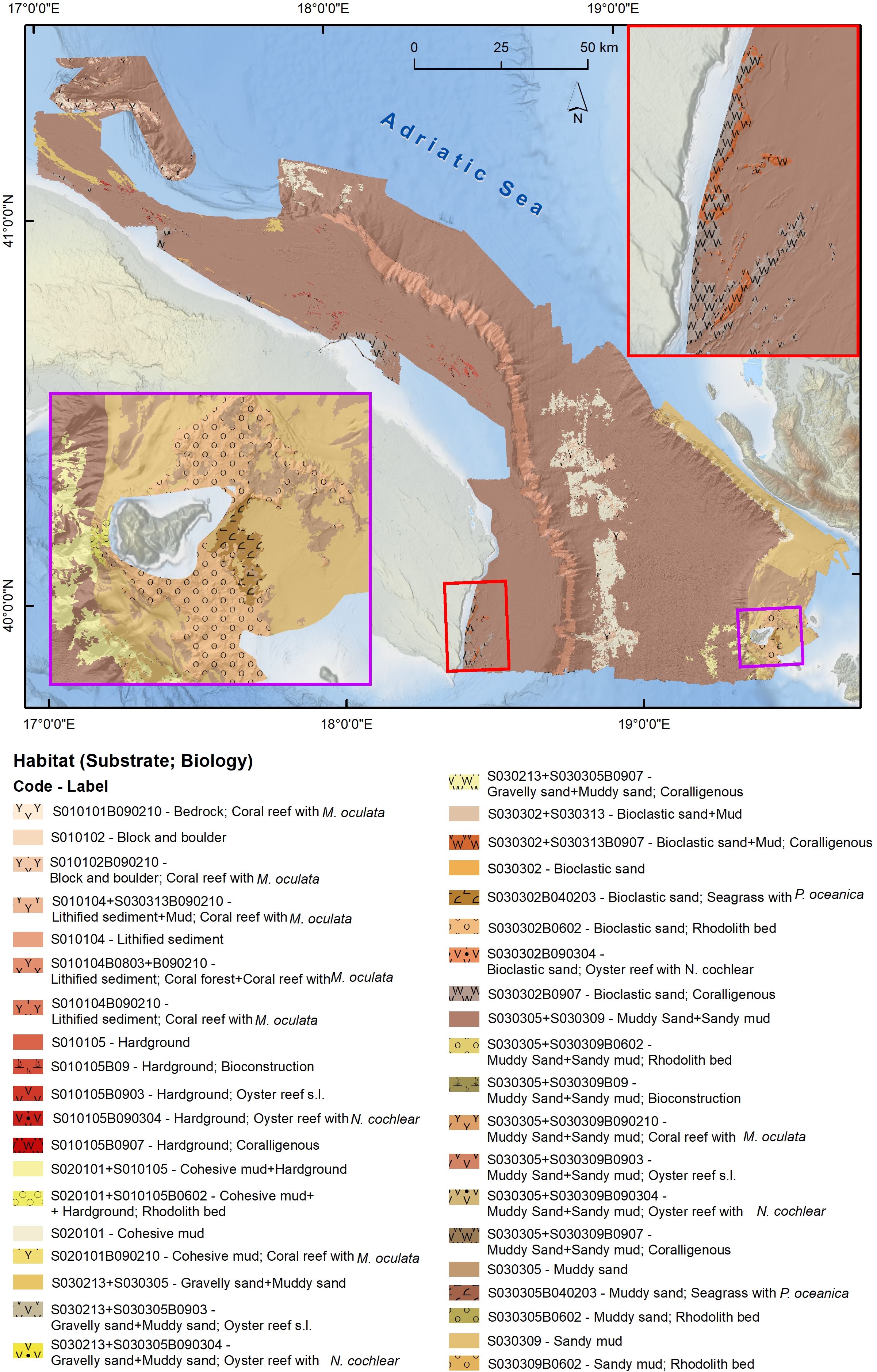
Figure 5. Substrate and Biology components of the South Adriatic continental margin classified according to CoDeMap BHCS (modified from Prampolini et al., 2021). Background: EMODnet Bathymetry World Base Layer version 1.

3.2 Tricase Canyon

The Tricase Canyon is a submarine feature that cuts through the Apulian continental slope on the western side of the Ionian Sea (Mediterranean Sea). Morphological and substrate components were mapped by interpreting the Digital Elevation Model (DEM) and classifying seabed acoustic reflectivity using Remote Sensor Object-Based Image Analysis (RSOBIA). A ground-truthing activity involving seabed samples and ROV images validated the results of the automatic classification and helped analyze the biological component. In fact, the deeper areas of the canyon host white corals such as Madrepora oculata, Desmophyllum dianthus, and Desmophyllum pertusum (=Lophelia pertusa). Corals have been mainly observed on the top of blocks interpreted as the result of several mass-transport deposits (Prampolini et al., 2020). Figure 6 shows the benthic habitat map of the Tricase Canyon described using the CoDeMap BHCS.

Figure 6

Figure 6. Benthic habitat map of the Tricase Canyon classified according to CoDeMap (codes explanation is given in Table 2). Colors represent the morphologies of the canyon (yellow tones for the continental shelf, orange-green tones for the continental slope and blue tones for the basin plain); the pattern of the polygons corresponds to a specific substrate that is red when also the biological component is present. Background: EMODnet Bathymetry World Base Layer version 1.

For the Tricase Canyon case, we decided to use all 11 levels in the legend displaying just the code, integrating all three components into a single seafloor representation. Table 2 contains the labels for the various classes.

Table 2

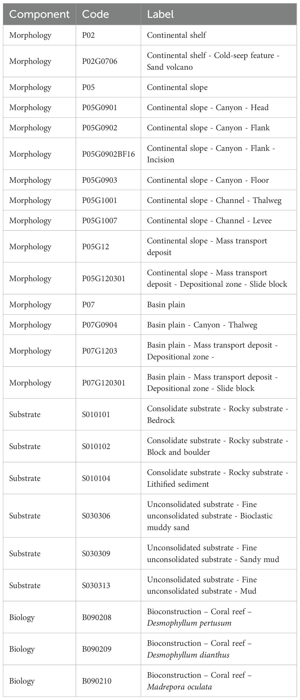
Table 2. Description of the codes used in the legend of Figure 6.

3.3 ROV transect in the Dohrn Canyon

The Dohrn Canyon is in the center of the Gulf of Naples, a submarine canyon of ecological, functional and oceanographic interest since featured by important upwelling currents affecting more coastal waters. It hosts deep bioconstructions, specifically cold-water corals and oysters. Available information documents the presence of living specimens of the scleractinians M. oculata, D. pertusum, and D. dianthus. These communities are also associated with large bivalves such as Neopycnodonte zibrowii and Acesta excavata. This coexistence of deep corals and large bivalves represents a unique biotope for the Mediterranean Sea, threatened by severe anthropogenic threats (Taviani et al., 2019).

In this application of the CoDeMap BHCS, we described the ROV transect coded “ANOMCITY_ROV01”, conducted during the CNR oceanographic cruise ANOMCITY 2016 aimed to characterize and map the bioconstructions populating the Dohrn Canyon (Oliveri et al., 2016). The transect develops along the flank of the northern branch of the canyon following a South-North direction, revealing the coexistence of cold-water corals and deep oysters (Figure 7).

Figure 7

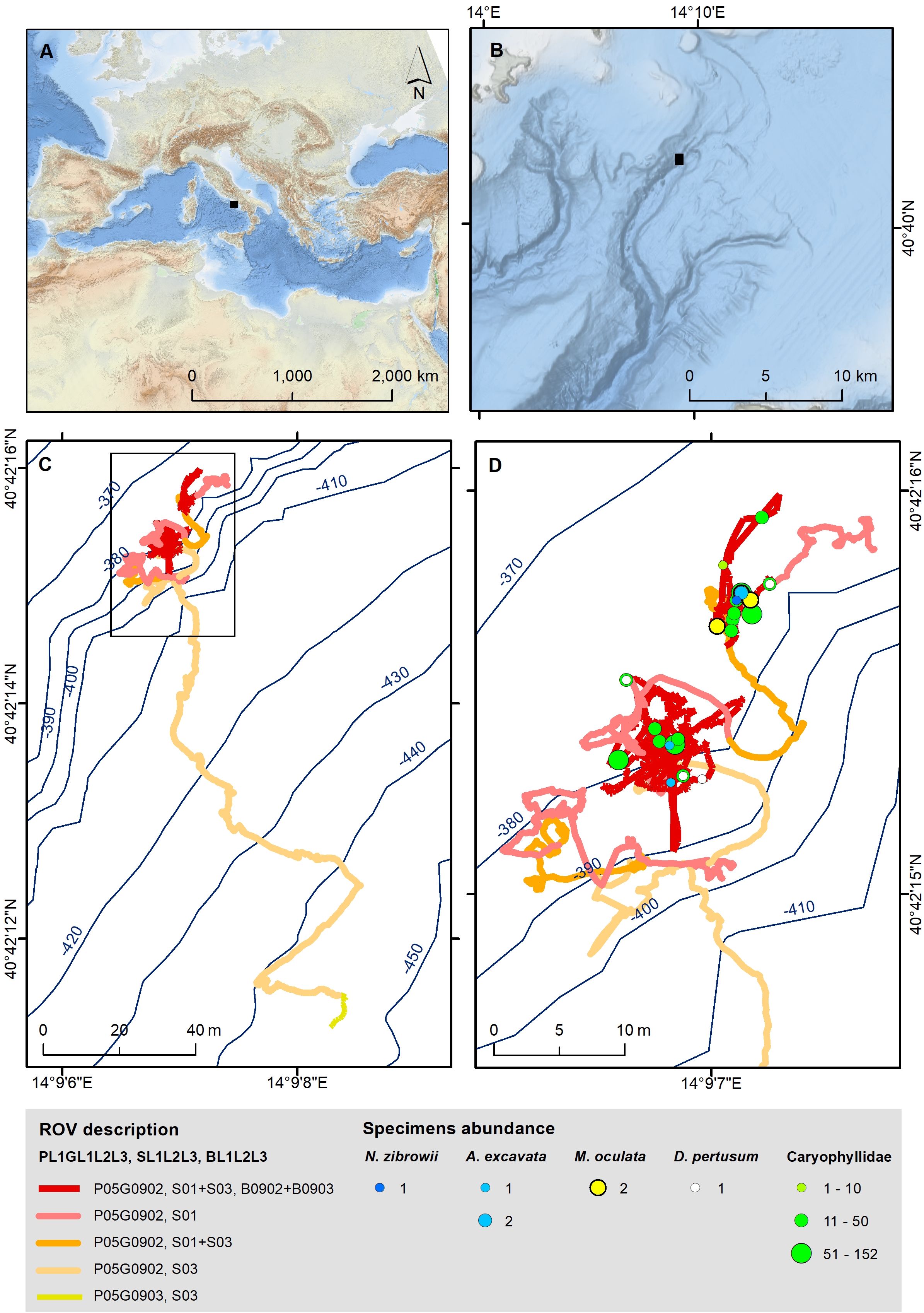
Figure 7. (A, B) show the location of the ROV transect ANOMCITY_ROV01 in the Mediterranean Sea and in the Dohrn Canyon, respectively. In (C), the seafloor is described using the three components of the CoDeMap BHCS. (D) shows a zoom in the rocky part of the transect hosting cold-water corals (B0902 - Bioconstructions, Coral reef) and deep oyster (B0903 - Bioconstruction, Oyster s.l. reef). Point size refers to the abundance of specimens.

3.4 Continental shelf along the Apulian coast

From 2000 to 2024 several research projects and scientific papers focused on the area in the South Adriatic Sea that runs along the Apulian coast and continental shelf (Italy). In this case study, we considered the seabed stretching from Mola di Bari to Fasano municipalities hosting Posidonia oceanica meadows, coralligenous bioconstructions and coral reefs in shallow waters, as well as deep oyster reefs in the continental shelf at approximately at 100 meters water depth. The seabed substrate ranges from hardgrounds to bioclastic coarse and fine sediments (from gravelly sands to sandy muds), while the continental shelf is characterized by flat surfaces, megaripple fields, comet marks, and erosional remnants. We integrated the maps produced through the years from the coast to the deep-sea into a comprehensive map intended to support conservation initiatives, such as the establishment of new Natura 2000 sites (Grande et al., 2024). The main challenge lies in homogenizing maps derived from multiple sources, produced at different scales and using different devices (see Supplementary Figure S1 in the Supplementary Materials for the original data).

Figure 8 compares the CoDeMap and EUNIS classification schemes in the production of benthic habitat maps for Apulian coastal waters and continental shelf. Both frameworks ensure a consistent representation of the study area, even in contexts where data availability is limited. Within EUNIS, these areas can be classified at Level 1 as “Marine benthic habitats,” whereas CoDeMap adds further detail by incorporating physiographic features such as the “Continental shelf.” The key distinction between the two approaches lies in the reliance on biozones in EUNIS versus geomorphological classes in CoDeMap. In Figure 8A, geomorphological features are clearly delineated, with biological data embedded within their abiotic setting. For instance, the oyster reef offshore Monopoli is shown to coincide with an erosive remnant area, offering valuable insights into the reef’s formation. Conversely, EUNIS highlights the spatial distribution of biozones: Figure 8B clearly illustrates the extent of habitats across the infralittoral and circalittoral zones.

Figure 8

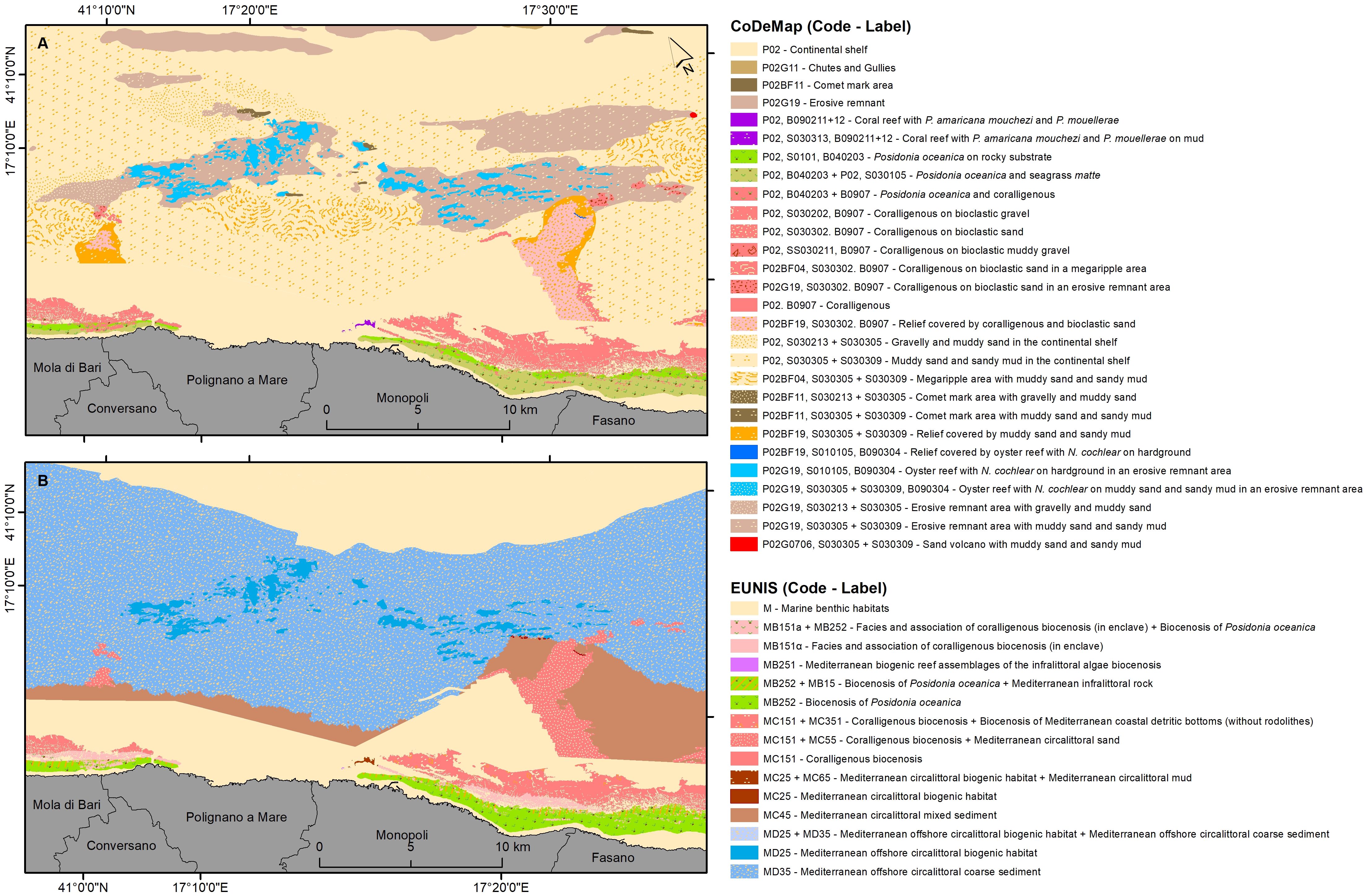
Figure 8. Comparison between the CoDeMap and EUNIS classification schemes applied on the South Adriatic Sea continental shelf along the Apulian coast (Italy). (A) represents the benthic habitats classified according to the CoDeMap BHCS, and (B) the same habitats classified according to the EUNIS classification scheme.

In terms of completeness, CoDeMap generally provides a more detailed account of the original data. This is exemplified by the mesophotic coral reef described by Corriero et al. (2019), classified under CoDeMap as a coral reef dominated by Phyllangia americana mouchezii and Polycyathus muellerae, whereas EUNIS categorizes it as “MC2 – Mediterranean circalittoral biogenic habitat.” In this case, the absence of specific EUNIS classes necessitates classification at Level 3, resulting in a coarser description. By contrast, CoDeMap captures the reef’s character more precisely, including the identification of its dominant species.

When harmonizing maps from different sources, however, some information may be lost, potentially leading to misclassification or the use of categories that do not fully match the context. This is illustrated in Figure 8 with the mapping of Posidonia oceanica from the “Inventory and Cartography of Posidonia Meadows” (POR 2000–2006). The dataset shows a mosaic of Posidonia oceanica and matte within the circalittoral zone. Under the EUNIS scheme, the area can only be mapped as MB252 “Biocenosis of Posidonia oceanica” (Figure 8B), which omits details on the presence of matte, since the available data are insufficient to classify the habitat at Level 5 (e.g., MB2523 “Facies of dead mattes of Posidonia oceanica without much epiflora”). CoDeMap, by contrast, allows classes to be combined, thus retaining the full complexity of the original dataset.

Finally, CoDeMap consistently provides detailed information on substrate composition (e.g., gravelly and muddy sands or sandy muds across the continental shelf), whereas EUNIS categories do not always capture substrate variability exhaustively—for example, “MC45 Mediterranean circalittoral mixed sediment”.

4 Discussion

Over the past few decades, numerous classification systems have been developed, resulting in a variety of schemes and lists that are used for habitat description and monitoring. Many of these are incompatible among each other, making it difficult to compare habitat types across studies and regions (Fraschetti et al., 2024; Greene et al., 2008). The selection of the classification system to map benthic habitats is dependent on national preferences, established practices, and user expertise. Classifying natural continuities and environmental gradients into discrete and meaningful categories is a challenging endeavor, as it imposes constraints and limitations on the natural variability of ecological communities. Consequently, multiple BHCSs exist, differing in (i) purpose; (ii) environmental and ecological scope; (iii) spatial scale; (iv) thematic resolution; (v) structure; and (vi) compatibility for habitat mapping. Variations in these properties can significantly influence the presence and representation of marine habitat distributions (Strong et al., 2019).

CoDeMap is hierarchical and multiscale, adaptable to data availability and to the scale of work, and it is easy to manage and apply in a GIS environment. By using the CoDeMap BHCS, it is possible to map the different components of the benthic habitats separately and at different scales as shown in the application “South Adriatic continental margin” (Figures 3–5). This ensures the production of continuous maps for one or more components, regardless of the quality or quantity of the available data. Components can be combined to produce a benthic habitat map to get a full picture of a marine seafloor as demonstrated in the “Tricase Canyon” (Figure 6) or according to detailed levels (Figure 7). It is important to note that the resolution achievable within each component and level depends on the means and techniques employed for habitat mapping. For instance, the use of multibeam echosounder (MBES) data generally allows reliable classification of seafloor morphology down to the Geoform and Bedform levels (GL1–3, BFL1), whereas sediment samples and ground-truthing techniques are essential to resolve Substrate levels (SL2–3). Similarly, biological samples or seabed pictures are typically required to define the Biology component (BL1–3), with biological samples necessary to reach the most detailed level of biology (BL3). Thus, the scheme provides a flexible framework where the depth of classification is directly related to the type and resolution of the available data.

Habitat mapping is a multidisciplinary endeavor, requiring collaboration among geologists, biologists, and other specialists. However, the modular structure of the CoDeMap scheme—organized into separate components—enables users to apply it according to their own expertise. For instance, if a geologist is unable to classify the biological component, the output will consist of a map of seabed morphology and substrate, which can later be complemented with biological information once a collaboration with biologists is established. Conversely, a biologist can map the biological component, with geological features subsequently added in partnership with geologists. This flexibility is not possible with classification schemes based on predefined combinations of components: a geologist would struggle to select among classes that share the same morphology and substrate but differ in biological communities, while a biologist would face difficulties distinguishing between classes defined by the same community but varying morphological or substrate characteristics.

In addition to scale and data availability, another driver in the application of CoDeMap can be the user purpose. If the focus is on geology, for instance, the morphology of the benthic habitat map can be the primary information displayed resulting in a continuous, colorful basemap, as illustrated in Figure 4. If the emphasis is on biology, substrate can be used as background element, then highlighting the biological elements layered on top (Figure 5). This is a great advantage because it allows the benthic habitat map representation to be updated or changed to suit the needs of any given project by simply accentuating a particular component above the others or by choosing the levels of interest. For example, in the application named “ROV transect in the Dohrn Canyon” (Figure 7), the goal was to describe the seafloor characteristics and the biological community along an ROV transect for monitoring and conservation purposes. Finally, the ability to build purpose-driven maps makes CoDeMap a valuable tool in decision-making processes for users with varying levels of expertise and diverse backgrounds. Thanks to its immediacy and simplicity in conveying information, policy makers can also take advantage of CoDeMap: it enables them to clearly represent the messages and priorities they wish to communicate, thus facilitating understanding and the sharing of strategic decisions.

Such flexibility makes CoDeMap a user-friendly tool, enabling the classification of seafloor at various degrees. The applications of the CoDeMap BHCS highlight the scheme’s versatility regarding spatial scale and code customization to suit the objectives of the representation. It is conceived as an evolving system that can be continuously enriched with new classes also to accommodate changes in future marine environments based on scientific community feedback (Albano et al., 2024; Coll et al., 2010; Thiébault and Moatti, 2016). In such a perspective, contributors can utilize a dedicated website (https://codemap.my.canva.site/about), where the latest version of the scheme is always accessible, and suggestions can be submitted.

5 Conclusions

In this work, we present CoDeMap, a classification scheme tailored for Mediterranean and Black Sea benthic habitats, ranging from coastal areas to the deep sea. CoDeMap offers a flexible framework for classifying marine benthic habitats suitable for GIS applications. It is rooted in scientific principles yet adaptable for various contexts, including citizen science, scientific research, and decision making. This study details the components, subcomponents, levels, and classes of CoDeMap, along with four diverse use cases that demonstrate the scheme’s versatility in a range of scenarios (from simple assessments to highly detailed representations), according to scale, data availability, and individual expertise and objectives. CoDeMap will undergo continuous updates to reflect the dynamic nature of benthic habitats and marine ecosystem changes.

Data availability statement

The maps used for GIS applications are freely accessible through the Geoportal for Marine Biodiversity in Italy, reachable via the Biodiversity Gateway (https://www.biodiversitygateway.it). The CoDeMap benthic classification scheme is available to download as an Excel file in the Supplementary Materials. Different versions and an online contribution form are accessible at the following link: https://codemap.my.canva.site/about.

Author contributions

VG: Conceptualization, Methodology, Software, Writing – original draft, Writing – review & editing, Validation. LA: Conceptualization, Writing – original draft, Writing – review & editing, Methodology, Validation. MP: Software, Writing – original draft, Writing – review & editing, Validation. GCa: Writing – original draft, Writing – review & editing, Validation. GV: Writing – original draft, Validation. SF: Conceptualization, Funding acquisition, Supervision, Writing – review & editing. DBa: Validation, Writing – review & editing. DBe: Validation, Writing – review & editing. VB: Validation, Writing – review & editing. FC: Validation, Writing – review & editing. GCh: Validation, Writing – review & editing. AF: Validation, Writing – review & editing. BG: Validation, Writing – review & editing. FM: Validation, Writing – review & editing. MS: Validation, Writing – review & editing. AS: Validation, Writing – review & editing. PS: Validation, Writing – review & editing. VT: Validation, Writing – review & editing. MT: Conceptualization, Writing – review & editing, Validation. FF: Conceptualization, Funding acquisition, Methodology, Supervision, Writing – review & editing.

Funding

The author(s) declare financial support was received for the research and/or publication of this article. This paper is CNR-ISMAR-Bologna scientific contribution n. 2091 and is part of EU F.P. VII Project CoCoNet (contract no. 287844), the Italian Flagship Project RITMARE, LIFE DREAM Project (LIFE21-NAT-IT-LIFE-DREAM/101074547), REDRESS Project (project no. 101135492), and the National Biodiversity Future Center - NBFC (funded under the National Recovery and Resilience Plan (NRRP), Mission 4 Component 2 Investment 1.4 - Call for tender No. 3138 of 16 December 2021, rectified by Decree n.3175 of 18 December 2021 of Italian Ministry of University and Research funded by the European Union – NextGenerationEU; Award Number: Project code CN_00000033, Concession Decree No. 1034 of 17 June 2022 adopted by the Italian Ministry of University and Research, CUP D33C22000960007).

Acknowledgments

The Authors are grateful to the CoCoNet Consortium that participated in the first draft of the classification scheme. This is ISMAR-CNR, Bologna, scientific contribution n. 2091.

Conflict of interest

The authors declare that the research was conducted in the absence of any commercial or financial relationships that could be construed as a potential conflict of interest.

The author(s) declared that they were an editorial board member of Frontiers, at the time of submission. This had no impact on the peer review process and the final decision.

Generative AI statement

The author(s) declare that no Generative AI was used in the creation of this manuscript.

Any alternative text (alt text) provided alongside figures in this article has been generated by Frontiers with the support of artificial intelligence and reasonable efforts have been made to ensure accuracy, including review by the authors wherever possible. If you identify any issues, please contact us.

Publisher’s note

All claims expressed in this article are solely those of the authors and do not necessarily represent those of their affiliated organizations, or those of the publisher, the editors and the reviewers. Any product that may be evaluated in this article, or claim that may be made by its manufacturer, is not guaranteed or endorsed by the publisher.

Supplementary material

The Supplementary Material for this article can be found online at: https://www.frontiersin.org/articles/10.3389/fmars.2025.1663369/full#supplementary-material

Supplementary Table S1 | CoDeMap benthic habitat classification scheme – version 1.0..

Supplementary Figure S1 | Data sources used for the case study “Comparison between CoDeMap and EUNIS classification schemes” paragraph 3.4. In red, the distribution of bioconstructions mapped in 2012 as part of the BIOMAP project (http://www.sit.puglia.it/portal/portale_rete_ecologica/biomap), and in yellow, the distribution of Posidonia oceanica along the Apulian coastline produced in 2004–2005 as part of the project “Inventory and Cartography of Posidonia Meadows in the Maritime Compartments of Manfredonia, Molfetta, Bari, Brindisi, Gallipoli and Taranto (POR 2000-2006)” (https://emodnet.ec.europa.eu/geonetwork/srv/ita/catalog.search#/metadata/e14e1bc8-e52b-4460-b5b3-b5550520728f). In purple, the distribution of mesophotic corals along the Apulian coastline published by Corriero et al. in 2019 (https://doi.org/10.1038/s41598-019-40284-4), and in green, the distribution of the deep oyster reef produced in the framework of the LIFE DREAM Project (Grande et al., 2024; https://doi.org/10.26383/CNR-ISMAR.2024.6). The area in lilac color is covered by the geomorphological map of the South Adriatic continental margin published in Campiani et al., 2024 (https://doi.org/10.1080/17445647.2024.2429707), and in orange, the benthic habitat map published by Prampolini et al., 2021 (https://doi.org/10.3390/rs13152913). The EMODnet Digital Bathymetry (DTM 2024) provides the background (in blue) and the isobaths (blue lines with 10 meters interval).

References

Albano P. G., Schultz L., Wessely J., Taviani M., Dullinger S., and Danise S. (2024). The dawn of the tropical Atlantic invasion into the Mediterranean Sea. Proc. Natl. Acad. Sci. U.S.A. 121, e2320687121. doi: 10.1073/pnas.2320687121

PubMed Abstract | Crossref Full Text | Google Scholar

Angeletti L., D’Onghia G., Otero M., del M., Settanni A., Spedicato M. T., et al. (2021). A perspective for best governance of the Bari Canyon deep-sea ecosystems. Water 13, 1646. doi: 10.3390/w13121646

Crossref Full Text | Google Scholar

Ashley G. M. (1990). Classification of large-scale subacqueous bedforms: a new look at an old problem. J. Sedimentary Petrology 60, 160–172. doi: 10.2110/jsr.60.160

Crossref Full Text | Google Scholar

Avellan L., Haldin J., Kontula K., Leinikki J., Näslund J., and Laamanen M. (2013). HELCOM HUB - Technical Report on the HELCOM Underwater Biotope and habitat classification (Baltic Sea Environment Proceedings No. 139 (Technical Report No. 139).

Google Scholar

Azzola A., Bavestrello G., Bertolino M., Bianchi C. N., Bo M., Enrichetti F., et al. (2021). You cannot conserve a species that has not been found: The case of the marine sponge Axinella polypoides in Liguria, Italy. Aquat. Conserv. 31, 737–747. doi: 10.1002/aqc.3492

Crossref Full Text | Google Scholar

Beca-Carretero P., Teichberg M., Winters G., Procaccini G., and Reuter H. (2020). Projected rapid habitat expansion of tropical seagrass species in the mediterranean sea as climate change progresses. Front. Plant Sci. 11. doi: 10.3389/fpls.2020.555376

PubMed Abstract | Crossref Full Text | Google Scholar

Bekkby T., Papadopoulou N., Fiorentino D., McOwen C. J., Rinde E., Boström C., et al. (2020). Habitat features and their influence on the restoration potential of marine habitats in europe. Front. Mar. Sci. 7. doi: 10.3389/fmars.2020.00184

Crossref Full Text | Google Scholar

Bellin N. and Rossi V. (2024). Modeling the effects of climate change on the habitat suitability of Mediterranean gorgonians. Biodivers Conserv. 33, 1027–1049. doi: 10.1007/s10531-024-02779-z

Crossref Full Text | Google Scholar

Bianchi C., Parravicini V., Montefalcone M., Rovere A., and Morri C. (2012). The challenge of managing marine biodiversity: A practical toolkit for a cartographic, territorial approach. Diversity 4, 419–452. doi: 10.3390/d4040419

Crossref Full Text | Google Scholar

Brown C. J., Smith S. J., Lawton P., and Anderson J. T. (2011). Benthic habitat mapping: A review of progress towards improved understanding of the spatial ecology of the seafloor using acoustic techniques. Estuarine Coast. Shelf Sci. 92, 502–520. doi: 10.1016/j.ecss.2011.02.007

Crossref Full Text | Google Scholar

Butler C., Lucieer V., Walsh P., Flukes E., and Johnson C. (2017). Seamap Australia [Version 1.0] the development of a national benthic marine classification scheme for the Australian continental shelf (Hobart, Australia: The Institute for Marine and Antarctic Studies, University of Tasmania). doi: 10.25607/OBP-459

Crossref Full Text | Google Scholar

Campiani E., Trincardi F., Foglini F., Dalla Valle G., Leidi E., Mercorella A., et al. (2024). Geohazard features of the Central Apulia. Journal of Maps 20 (1). doi: 10.1080/17445647.2024.2429707

Crossref Full Text | Google Scholar

Cogan C. B., Todd B. J., Lawton P., and Noji T. T. (2009). The role of marine habitat mapping in ecosystem-based management. ICES J. Mar. Sci. 66, 2033–2042. doi: 10.1093/icesjms/fsp214

Crossref Full Text | Google Scholar

Coggan R., Populus J., White J., Sheehan K., Fitzpatrick F., and Piel S. (2007). Review of Standards and Protocols for Seabed Habitat Mapping. 2ª ed (Peterborough, UK: Mapping European Seabed Habitats (MESH).

Google Scholar

Coll M., Piroddi C., Steenbeek J., Kaschner K., Ben Rais Lasram F., Aguzzi J., et al. (2010). The biodiversity of the mediterranean sea: estimates, patterns, and threats. PLoS One 5, e11842. doi: 10.1371/journal.pone.0011842

PubMed Abstract | Crossref Full Text | Google Scholar

Corriero G., Pierri C., Mercurio M., Nonnis Marzano C., Onen Tarantini S., Gravina M. F., et al (2019). A Mediterranean mesophotic coral reef built by non-symbiotic scleractinians. Sci. Rep. 9, 3601. doi: 10.1038/s41598-019-40284-4

PubMed Abstract | Crossref Full Text | Google Scholar

Danovaro R., Fanelli E., Canals M., Ciuffardi T., Fabri M.-C., Taviani M., et al. (2020). Towards a marine strategy for the deep Mediterranean Sea: Analysis of current ecological status. Mar. Policy 112, 103781. doi: 10.1016/j.marpol.2019.103781

Crossref Full Text | Google Scholar

Davies J. S., Guillaumont B., Tempera F., Vertino A., Beuck L., Ólafsdóttir S. H., et al. (2017). A new classification scheme of European cold-water coral habitats: Implications for ecosystem-based management of the deep sea. Deep Sea Res. Part II: Topical Stud. Oceanography 145, 102–109. doi: 10.1016/j.dsr2.2017.04.014

Crossref Full Text | Google Scholar

Davies C. E. and Moss D. (1998). EUNIS habitat classification (Brussels, European: European Topic Centre on Nature Conservation, European Environment Agency).

Google Scholar

Davies C. E., Moss D., and Hill M. O. (2004). Eunis Habitat Classification Revised 2004 (European Environment Agency - European Topic Centre on Nature Protection and Biodiversity).

Google Scholar

Diaz R. J., Solan M., and Valente R. M. (2004). A review of approaches for classifying benthic habitats and evaluating habitat quality. J. Environ. Manage. 73, 165–181. doi: 10.1016/j.jenvman.2004.06.004

PubMed Abstract | Crossref Full Text | Google Scholar

Dove D., Nanson R., Bjarnadóttir L. R., Guinan J., Gafeira J., Post A., et al. (2020). A two-part seabed geomorphology classification scheme (v.2); Part 1: morphology features glossary. Zenodo, 23. doi: 10.5281/ZENODO.4075248

Crossref Full Text | Google Scholar

Enrichetti F., Dominguez-Carrió C., Toma M., Bavestrello G., Canese S., and Bo M. (2020). Assessment and distribution of seafloor litter on the deep Ligurian continental shelf and shelf break (NW Mediterranean Sea). Mar. pollut. Bull. 151, 110872. doi: 10.1016/j.marpolbul.2019.110872

PubMed Abstract | Crossref Full Text | Google Scholar

Fraschetti S., Guarnieri G., Bevilacqua S., Terlizzi A., Claudet J., Russo G. F., et al. (2011). Conservation of Mediterranean habitats and biodiversity countdowns: what information do we really need? Aquat. Conserv. 21, 299–306. doi: 10.1002/aqc.1185

Crossref Full Text | Google Scholar

Fraschetti S., Strong J., Buhl-Mortensen L., Foglini F., Goncalves J. M. S., Goncalez-Irusta J. M., et al. (2024). “EMB Future Science Brief No. 11 “Marine habitat mapping,” in Future Science Brief N°. 11 of the European Marine Board. Eds. Alexander B., Rodriguez Perez A., Kellet P., Muñiz Piniella A., Bayo Ruiz F., Bairaktari K., and Heymans J. J. (Zenodo, Onstend, Belgium).

Google Scholar

Fraschetti S., Terlizzi A., and Boero F. (2008). How many habitats are there in the sea (and where)? J. Exp. Mar. Biol. Ecol. 366, 109–115. doi: 10.1016/j.jembe.2008.07.015

Crossref Full Text | Google Scholar

Galparsoro I. (2012). Using EUNIS habitat classification for benthic mapping in European seas: Present concerns and future needs. Mar. pollut. Bull. 9, 2630-2638. doi: 10.1016/j.marpolbul.2012.10.010

PubMed Abstract | Crossref Full Text | Google Scholar

Gerovasileiou V., Smith C. J., Sevastou K., Papadopoulou N., Dailianis T., Bekkby T., et al. (2019). Habitat mapping in the European Seas - is it fit for purpose in the marine restoration agenda? Mar. Policy 106, 103521. doi: 10.1016/j.marpol.2019.103521

Crossref Full Text | Google Scholar

Grande V., Angeletti L., Castellan G., Dalla Valle G., Foglini F., Prampolini M., et al. (2024). Proposta di ampliamento della Rete Natura 2000 in acque profonde nell’ambito del progetto LIFE DREAM. relazione d’inquadramento per la Regione Puglia. doi: 10.26383/CNR-ISMAR.2024.6

Crossref Full Text | Google Scholar

Greene H. G., Yoklavich M. M., Starr R. M., O’Connell V. M., Wakefield W. W., Sullivan D. E., et al. (1999). A classification scheme for deep seafloor habitats. Oceanologica Acta 22, 663–678. doi: 10.1016/S0399-1784(00)88957-4

Crossref Full Text | Google Scholar

Greene H. G., Bizzarro J. J., Tilden J. E., Lopez H. L., and Erdey M. D. (2005). “The benefits and pitfalls of geographic information systems in marine benthic habitat mapping,” in Place Matters: Geospatial Tools for Marine Science, Conservation, and Management in the Pacific Northwest. Eds. Wright D. J. and Scholz A. J. (Oregon State University Press, Corvallis, OR).

Google Scholar

Greene H., O’Connell V., Brylinsky C., and Reynolds J. (2008). “Marine benthic habitat classification: what’s best for Alaska?,” in Marine Habitat Mapping Technology for Alaska. Eds. Reynolds J. and Greene H. (Alaska Sea Grant, University of Alaska Fairbanks: Alaska Sea Grant College Program, University of Alaska Fairbanks), 169–184. doi: 10.4027/mhmta.2008.12

Crossref Full Text | Google Scholar

Guarinello M. L., Shumchenia E. J., and King J. W. (2010). Marine habitat classification for ecosystem-based management: A proposed hierarchical framework. Environ. Manage. 45, 793–806. doi: 10.1007/s00267-010-9430-5

PubMed Abstract | Crossref Full Text | Google Scholar

Guillaumont B., Tempera F., Davies J., Vertino A., Beuck L., Ólafsdóttir S. H., et al. (2016). CoralFish North-East Atlantic and Mediterranean cold-water coral habitats catalogue (Version 2) (Project deliverable No. Deliverable 49) (Reykjavik, Island: Zenodo).

Google Scholar

Harris P. T. and Baker E. K. (Eds.) (2020). Seafloor Geomorphology as Benthic Habitat - GeoHab Atlas of Seafloor Geomorphic Features and Benthic Habitats (Second Edition) (Amsterdam, The Netherlands: Elsevier).

Google Scholar

Harris P. T., Macmillan-Lawler M., Rupp J., and Baker E. K. (2014). Geomorphology of the oceans. Mar. Geology 352, 4–24. doi: 10.1016/j.margeo.2014.01.011

Crossref Full Text | Google Scholar

Holon F., Mouquet N., Boissery P., Bouchoucha M., Delaruelle G., Tribot A.-S., et al. (2015). Fine-scale cartography of human impacts along french mediterranean coasts: A relevant map for the management of marine ecosystems. PLoS One 10, e0135473. doi: 10.1371/journal.pone.0135473

PubMed Abstract | Crossref Full Text | Google Scholar

Keith D. A., Ferrer-Paris J. R., Nicholson E., and Kingsford R. T. (Eds.) (2020). IUCN Global Ecosystem Typology 2.0: descriptive profiles for biomes and ecosystem functional groups (Gland, Switzerland: IUCN, International Union for Conservation of Nature). doi: 10.2305/IUCN.CH.2020.13.en

Crossref Full Text | Google Scholar

Lucieer V., Walsh P., Flukes E., Butler C., Proctor R., and Johnson C. (2017). Seamap Australia - a national seafloor habitat classification scheme.

Google Scholar

Madden C., Goodin K., Allee B., Finkbeiner M., and Bamford D. (2009). Coastal and marine ecological classification standard (NOAA and NatureServe), 107.

Google Scholar

Martin C. S., Giannoulaki M., De Leo F., Scardi M., Salomidi M., Knittweis L., et al. (2014). Coralligenous and maërl habitats: predictive modelling to identify their spatial distributions across the Mediterranean Sea. Sci. Rep. 4, 5073. doi: 10.1038/srep05073

Crossref Full Text | Google Scholar

McQuaid K. A., Attrill M. J., Clark M. R., Cobley A., Glover A. G., Smith C. R., et al. (2020). Using habitat classification to assess representativity of a protected area network in a large, data-poor area targeted for deep-sea mining. Front. Mar. Sci. 7. doi: 10.3389/fmars.2020.558860

Crossref Full Text | Google Scholar

Micallef A., Krastel S., and Savini A. (Eds.) (2018). Submarine Geomorphology (Cham: Springer Geology. Springer International Publishing). doi: 10.1007/978-3-319-57852-1

Crossref Full Text | Google Scholar

Ministry of Fisheries and Department of Conservation (2008). Marine protected areas: classification, protection standard and implementation guidelines (Wellington, New Zealand: Ministry of Fisheries and Department of Conservation).

Google Scholar

Misiuk B. and Brown C. J. (2024). Benthic habitat mapping: A review of three decades of mapping biological patterns on the seafloor. Estuarine Coast. Shelf Sci. 296, 108599. doi: 10.1016/j.ecss.2023.108599

Crossref Full Text | Google Scholar

Montefalcone M., Tunesi L., and Ouerghi A. (2021). A review of the classification systems for marine benthic habitats and the new updated Barcelona Convention classification for the Mediterranean. Mar. Environ. Res. 169, 105387. doi: 10.1016/j.marenvres.2021.105387

PubMed Abstract | Crossref Full Text | Google Scholar

Moraitis M. L., Valavanis V. D., and Karakassis I. (2019). Modelling the effects of climate change on the distribution of benthic indicator species in the Eastern Mediterranean Sea. Sci. Total Environ. 667, 16–24. doi: 10.1016/j.scitotenv.2019.02.338

PubMed Abstract | Crossref Full Text | Google Scholar

Mount R., Bricher P., and Newton J. (2007). National Intertidal/Subtidal Benthic (NISB) Habitat Classification Scheme - Version 1.0. Australia: Australian Coastal Vulnerability Project, National Land & Water Resources Audit.

Google Scholar

Oliveri E., Bonsignore M., Canesi S., Castellan G., Cardone F., D’Agostino F., et al. (2016). Campagna oceanografica Anomcity_2016 [WWW Document] (URL http://eprints).

Google Scholar

Pérès J.-M. (1967). “The Mediterranean benthos,” in Oceanography and Marine Biology - An Annual Review. Ed. Barnes H. B. (George Allen & Unwin, London, UK), 449–533.

Google Scholar

Pérès J.-M. and Picard J. (1964). Nouveau manuel de bionomie benthique de la mer Méditerranée (Marseille, France: Station Marine d’Endoume).

Google Scholar

Prampolini M., Angeletti L., Castellan G., Grande V., Le Bas T., Taviani M., et al. (2021). Benthic habitat map of the southern adriatic sea (Mediterranean sea) from object-based image analysis of multi-source acoustic backscatter data. Remote Sens. 13, 2913. doi: 10.3390/rs13152913

Crossref Full Text | Google Scholar

Prampolini M., Angeletti L., Grande V., Taviani M., and Foglini F. (2020). “Chapter 48 - Tricase Submarine Canyon: cold-water coral habitats in the southwesternmost Adriatic Sea (Mediterranean Sea),” in Seafloor Geomorphology as Benthic Habitat, 2nd ed. Eds. Harris P. T. and Baker E. (Amsterdam, The Netherlands: Elsevier), 793–810. doi: 10.1016/B978-0-12-814960-7.00048-8

Crossref Full Text | Google Scholar

Robinson C. L. and Levings C. D. (1995). “An overview of habitat classification systems, ecological models, and geographic information systems applied to shallow foreshore marine habitats,” in Canadian Manuscript Report of Fisheries and Aquatic Sciences No. 2322. (Vancouver, Canada: Department of Fisheries and Oceans Science Branch, British Columbia, Canada).

Google Scholar

Rowden A. A., Lundquist C. J., Hewitt J. E., Stephenson F., and Morrison M. A. (2018). Review of New Zealand’s coastal and marine habitat and ecosystem classification (NIWA Client Report No. 2018115WN) (Wellington, New Zealand: NIWA).

Google Scholar

Schiele K. S., Darr A., and Zettler M. L. (2014). Verifying a biotope classification using benthic communities – An analysis towards the implementation of the European Marine Strategy Framework Directive. Mar. pollut. Bull. 78, 181–189. doi: 10.1016/j.marpolbul.2013.10.045

PubMed Abstract | Crossref Full Text | Google Scholar

Sokołowski A., Jankowska E., Balazy P., and Jędruch A. (2021). Distribution and extent of benthic habitats in Puck Bay (Gulf of Gdańsk, southern Baltic Sea). Oceanologia 63, 301–320. doi: 10.1016/j.oceano.2021.03.001

Crossref Full Text | Google Scholar

Standards Working Group - Federal Geographic Data Committee (2012). Coastal and Marine Ecological Classification Standard - Version 4.0.

Google Scholar

Strong J. A., Clements A., Lillis H., Galparsoro I., Bildstein T., and Pesch R. (2019). A review of the influence of marine habitat classification schemes on mapping studies: inherent assumptions, influence on end products, and suggestions for future developments. ICES J. Mar. Sci. 76, 10–22. doi: 10.1093/icesjms/fsy161

Crossref Full Text | Google Scholar

Taviani M., Angeletti L., Cardone F., Montagna P., and Danovaro R. (2019). A unique and threatened deep water coral-bivalve biotope new to the Mediterranean Sea offshore the Naples megalopolis. Sci. Rep. 9, 3411. doi: 10.1038/s41598-019-39655-8

PubMed Abstract | Crossref Full Text | Google Scholar

Templado J., Ballesteros E., Galparsoro I., Borja Á., Serrano A., Martín L., et al. (2012). Inventario español de hábitats y especies marinos. Guía interpretativa: inventario español de hábitats marinos. (Madrid, Spain: Ministerio de Agricultura, Alimentación y Medio Ambiente).

Google Scholar

Thiébault S. and Moatti J. P. (2016). The Mediterranean region under climate change: a scientific update (Marseille: IRD Éditions/AllEnvi).

Google Scholar

Valentine P. C., Todd B. J., and Kostylev V. E. (2005). “Classification of Marine sublittoral habitats, with application to the Northeastern North America Region,” in Benthic Habitats and the Effects of Fishing American Fisheries Society Symposium. Eds. Barnes P. W. and Thomas J. P. (American Fisheries Society Symposium), 183–200.

Google Scholar

Vassallo P., Bianchi C. N., Paoli C., Holon F., Navone A., Bavestrello G., et al. (2018). A predictive approach to benthic marine habitat mapping: Efficacy and management implications. Mar. pollut. Bull. 131, 218–232. doi: 10.1016/j.marpolbul.2018.04.016

PubMed Abstract | Crossref Full Text | Google Scholar

Ware S. and Downie A.-L. (2020). Challenges of habitat mapping to inform marine protected area (MPA) designation and monitoring: An operational perspective. Mar. Policy 111, 103717. doi: 10.1016/j.marpol.2019.103717

Crossref Full Text | Google Scholar

Wentworth C. K. (1922). A scale of grade and class terms for clastic sediments. J. Geology 30, 377–392. doi: 10.1086/622910

Crossref Full Text | Google Scholar