Abstract
The Yalu River Estuary (YRE) coastal wetland, as a vital part of the Yellow Sea Large Marine Ecosystem, provides habitats for hundreds of thousands of wintering waterfowl and millions of migratory shorebirds along the East Asian-Australasian Flyway. Given the accelerated rate of wetland loss during the 20th and early 21st centuries worldwide, effectively monitoring the dynamic changes of the wetlands is critical for adaptive wetland management. This study utilized Landsat TM/OLI images in 1990, 2000, 2011, and 2021 as data sources, employing an object-oriented random forest model classification approach to analyze the dynamic changes of each wetland type in the YRE coastal wetland over the past 31 years. The results showed that: 1) the object-oriented random forest model achieved high accuracy in classifying wetland types in the study area, with an overall classification accuracy exceeding 88%; 2) shallow marine waters, tidal wetlands, aquaculture ponds, and paddy fields are the predominant wetland types over the years, distributed in bands successively along the coastline, from the sea to the land; 3) compared with 1990, natural wetlands in YRE were degraded by 2021 with a decrease of 1,880.93 hm2; 4) the total area of natural and artificial wetlands remained relatively stable, due to the conversion of natural wetlands to artificial wetlands related to the development of agricultural, forestry, and fishery industries. The study indicates the reliability and efficiency of the application of the object-oriented random forest model classification approach on wetland monitoring. The trend of wetland change underscores the effectiveness of the reserve’s establishment.
1 Introduction
Coastal wetlands are the transition zones between the terrestrial ecosystem and the marine ecosystem, which play an important and unique role in regulating climate, preserving biodiversity, preventing disasters, and serving high ecological and economic benefits for local livelihood. However, in recent decades, wetland loss and damage have been constantly happening due to urban expansion, reclamation, coastal erosion, and destruction, causing ecological imbalance and functional degradation (Davidson, 2014; Sun et al., 2015). There has been a much (3.7 times) faster rate of wetland loss during the 20th and early 21st centuries, with a loss of 64%–71% of wetlands since 1900 AD (Davidson, 2014). Understanding the state of wetland ecosystems and their changes at the national and local levels is critical for wetland conservation, management, decision-making, and policy development practices. While large-scale mapping of coastal tidal wetland changes is extremely difficult due to their inherent dynamic nature, remote sensing and geographic information systems (GIS) technologies have emerged as efficient tools for wetland monitoring and assessment and have been evolving toward more effectiveness and high accuracy (Kashaigili et al., 2006; Whyte et al., 2018; Zekarias et al., 2021; Yang et al., 2022; Wang et al., 2023).
Bird surveys in the last two decades have highlighted the importance of tidal wetlands in the Yellow Sea for migratory shorebirds, with over 3 million shorebirds staying in the Yellow Sea during spring and autumn migration (Barter, 2002; MacKinnon et al., 2012). The North Yellow Sea is an important refueling site. Shorebird individuals stay in the North Yellow Sea for a long period and deposit large amounts of fuel with a high refueling rate (Hua, 2014). The Yalu River Estuary (YRE) coastal wetland located along the west side of the mouth of Yalu River, as the only coastal wetland in the middle temperate zone in China, provides habitats for hundreds of thousands of wintering waterfowl and millions of migratory shorebirds along the East Asian-Australasian Flyway (Barter et al., 2000; Ma et al., 2013; Hua, 2014; Hua et al.,2015). It supports some 250,000 shorebirds on northward migration, is of international importance for 17 shorebird species (Bai et al., 2015), and has become the main stopover for the great knot (Calidris tenuirostris) and bar-tailed godwit (Limosa lapponica) after the reclamation of Saemangeum wetland in South Korea (MacKinnon et al., 2012; Choi et al., 2015). The YRE was listed in conservation sites in 1987, when it was officially approved as a county nature reserve; in 1997, it was upgraded to a national nature reserve to maintain the coastal wetland ecosystem and protect the shorebirds; and in 1999, it was listed in the East Asia-Australia bird network officially by the Wetland International-Asia Pacific Council Management Committee.
However, there is limited research on the long-term monitoring of YRE over the past decades, which is essential for making informed decisions on conservation strategies. The previous works mostly took the YRE coastal wetland as a typical part in nationwide scope (Jiang et al., 2015; Wang et al., 2020) or part of the Yellow Sea (Yim et al., 2018; Chen et al., 2018), and either a holistic spatial dynamic analysis could not be given (Wu et al., 2021) or they only focused on narrow time periods before 2010 (Xu et al., 2006; He et al., 2009; Guo et al., 2014; Zhang et al., 2014).
In this regard, we use Landsat remote sensing images in 1990, 2000, 2011, and 2021 as data sources and the object-oriented random forest model classification method to extract wetland type information, while field survey data, historical data, and recent high-resolution data were utilized for verification. Then, we constructed the dynamic attitude model and Markov transfer matrix to illustrate the spatial dynamics of the wetland in the past three decades. This study makes a significant contribution by employing the object-oriented random forest model classification method and formulating long-term monitoring datasets for YRE, providing a more comprehensive view of conservation effectiveness and strategy than previous works.
2 Materials and methods
2.1 Study area
The Yalu River Estuary coastal wetland (123°35′E–124°08′E, 39°40′N–39°56′N) lies in Dandong City, the northernmost point of China’s coastline (Figure 1). The area is traversed by several rivers, including the Yalu River, Dayang River, Longtai River, and Zaoer Ditch. The area has a suitable water temperature, abundant sunshine, and a climate characterized by simultaneous rainy and hot seasons, providing good conditions for the growth and development of plants, as well as a variety of habitats for animals. There are 362 species of plants and 465 species of wild animals recorded in the area, including national key protected plants such as wild soybean, ginkgo, spruce, etc. and the national first- and second-class protected birds such as black-billed gull (Chroicocephalus bulleri), streak-backed marsh warbler (Locustella pryeri), red-crowned cranes (Grus japonensis), and white-naped cranes (Antigone vipio) (Xu et al., 2006), some of which are listed in the IUCN Red List of Threatened Species. The National Nature Reserve was designated into functional zones, including the core area, buffer area, and experimental area.
Figure 1
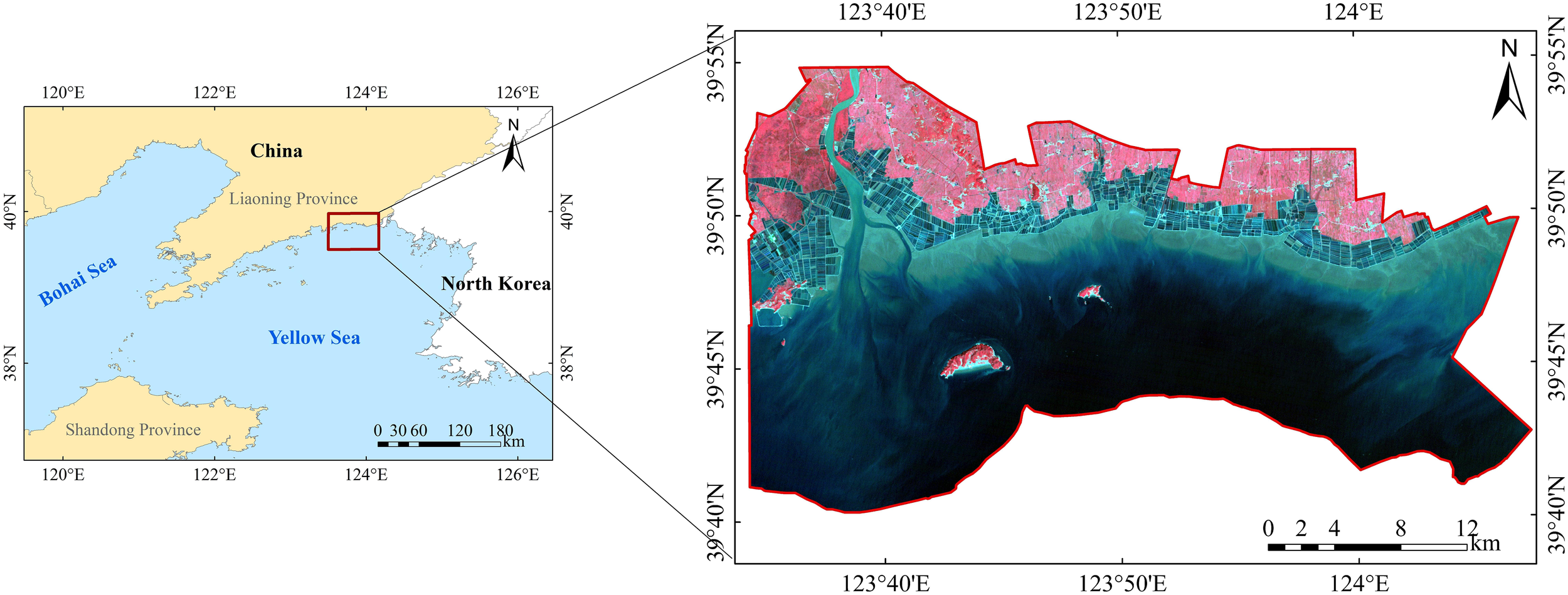
The location of the study area. The image is of standard false color synthesis using a 2000 Landsat image. The boundary of the study area is obtained by vectorizing the function zoning map of the Yalu River Estuary Coastal Wetland National Nature Reserve.
2.2 Remote sensing data
The Landsat satellite images used in this study were downloaded from the United States Geological Survey website (https://earthexplorer.usgs.gov/). Images from four time periods (1990, 2000, 2011, and 2021) were selected based on their image quality, season consistency, and minimal cloud cover (less than 5%) (Table 1).
Table 1
| Data source | Month-date-year | Orbit | Resolution (m) | Cloud cover (%) |
|---|---|---|---|---|
| Landsat OLI | 08-19-2021 | 118/32 | 30 | 3.22 |
| Landsat TM | 10-11-2011 | 118/32 | 30 | 0 |
| Landsat TM | 09-10-2000 | 118/32 | 30 | 0 |
| Landsat TM | 09-15-1990 | 118/32 | 30 | 0 |
Landsat images used in this study.
2.3 Data processing and analysis
2.3.1 Data preprocessing
Landsat images underwent radiometric calibration and atmospheric correction using the FLAASH tool in ENVI 5.3 software. According to the use of the band and the vector boundary of the nature reserve, images were synthesized in standard false color and cropped.
The classification of Landsat images mainly included the determination of the wetland classification system, construction of the classification method and classification process, etc. The specific technical route is shown in Figure 2.
Figure 2
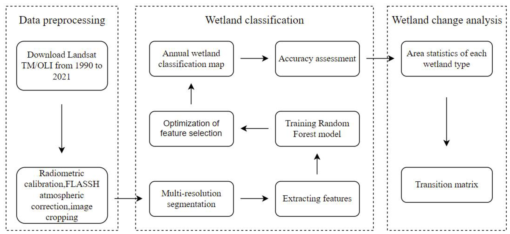
Flowchart of the research.
2.3.2 Wetland classification
Wetland classification is the basis of wetland research. In order to determine the YRE coastal wetland types and imagery interpretation marks, verify the scope of the YRE coastal wetland, and grasp the ecological environment problems, we conducted a field investigation from the 23rd to the 26th of September 2021. We used a handheld GPS to identify the wetland types in the study area and recorded these in a form that clarified the surface coverage characteristics and corresponding image characteristics of wetland types and non-wetland types, laying a foundation for the establishment of image interpretation signs.
Combined with the classification principles of coastal wetlands (Lu, 1990; Zhao and Wang, 2000) and previous research results (He et al., 2009), the wetland land use/cover classification system in the study area was first divided into three categories: natural wetland, artificial wetland, and non-wetland. Among them, natural wetlands were further divided into four types: reed wetland, river wetland, shallow marine water, and tidal wetland; artificial wetlands were classified into paddy field, salt flat, reservoir/pond, ditch, and aquaculture pond; and non-wetlands included forestland and construction land (Table 2).
Table 2
| First class | Second class | Description | Image feature |
|---|---|---|---|
| Natural wetland | Reed wetland | A marsh dominated by reed |

|
| River wetland | Natural river waters |

|
|
| Shallow marine water | Permanent marine water not exceeding a depth of 6 m at low tide |

|
|
| Tidal wetland | Intertidal silt beach |

|
|
| Artificial wetland | Paddy field | Mainly rice paddy field |

|
| Salt flat | Artificial ponds to extract salts from seawater |

|
|
| Reservoir/pond | Artificial water storage facility |

|
|
| Ditch | An artificial river or canal built to carry water |

|
|
| Aquaculture pond | Ponds for fishery cultivation |

|
|
| Non-wetland | Forestland | Land covered by natural forests or plantations |

|
| Construction land | Land for residential areas, roads, facilities, etc. |

|
Wetland classification system of the Yalu River coastal wetland.
2.4 Research method
2.4.1 Wetland classification method and accuracy assessment
Object-based image analysis (OBIA) has been widely recognized as an effective paradigm for processing remote sensing imagery (Blaschke, 2010). The random forest (RF) algorithm, an ensemble learning method based on decision trees proposed by Breiman (2001), has demonstrated strong robustness and computational efficiency within the OBIA framework, particularly in handling high-dimensional feature spaces (Ma et al., 2017). The integration of OBIA and RF has been extensively applied and validated in wetland mapping and monitoring, yielding reliable and reproducible results across diverse ecological contexts (Zhou et al., 2021; Granger et al., 2021). In this study, we employed an object-oriented random forest model for wetland classification, which was implemented through five main methodological phases.
2.4.1.1 Multiresolution segmentation
The eCognition software was used for multiresolution segmentation of images. In order to ensure the accuracy of interpretation of results, segmentation parameters and the optimal segmentation scale and the combination scale were obtained by the trial-and-error method: the segmentation scale was 60, the combination scale was 40, the compactness factor was 0.5, the shape factor was 0.1, and the band weight was 1.
2.4.1.2 Extracting features
On the basis of image segmentation, spectral, texture, exponential, and geometric features were extracted based on the segmented object to form a feature variable dataset (Sun, 2016) (Table 3). In addition, training samples were selected from them, which was critical for generating a transition matrix. Thus, training sample selection adhered to the principles of uniform distribution while actively excluding other ground objects, ensuring accurate class representation.
Table 3
| Feature type | Feature name | Feature abbreviation | Feature description |
|---|---|---|---|
| Spectral signature | Mean | B | The gray mean value of all pixels in each band |
| Standard deviation | Std_B | Standard deviation of gray values of all pixels in each band | |
| Brightness | Brightness | Weighted average of the gray values of each band within the object | |
| Max.Diff | Max.Diff | The maximum difference between the gray mean values of each band in the object | |
| Index feature | MNDWI | MNDWI | MNDWI = |
| NDVI | NDVI | NDVI = | |
| Geometric feature | Area | A | The total number of pixels contained within the image object |
| Length | L | The length of the image object along the long axis | |
| Length/Width | L/W | The ratio of length to width of the image object | |
| Compactness | C | The compactness of the image object | |
| Rectangular fit | RecF | Degree of fitting between the image object and a similar rectangle | |
| Shape index | SI | The smoothness of the object boundary | |
| Textural feature | GLCM homogeneity | Homogeneity | The inherent differences of image objects |
| GLCM contrast | Contrast | The degree of change in the image object | |
| GLCM Dissimilarity | Dissimilarity | The degree of gray detail change in the image object | |
| GLCM entropy | Entropy | The amount of information in the image object | |
| GLCM Ang.2nd moment | Ang.2nd moment | The uniformity of the gray distribution in the image object | |
| GLCM mean | Mean | The average gray value of the image object | |
| GLCM StdDev | StdDev | The grayscale variation of the image object. | |
| GLCM correlation | Correlation | The degree of linear correlation of the gray level in the image object |
Dataset of the extracted feature.
2.4.1.3 Training a random forest model
The MATLAB software was used to implement the random forest method for training the samples and constructing the dataset based on the optimal segmentation scale. The model was configured with 100 trees, using 1,700 test samples and 240 validation samples selected based on field surveys and image features. The sample selection ensured clarity, with no contamination from other land types, and the distribution was representative. After training and testing, the model achieved an accuracy of 94.80%. Upon completion of sample training, feature importance was evaluated, and the importance scores were ranked in descending order (Figure 3).
Figure 3
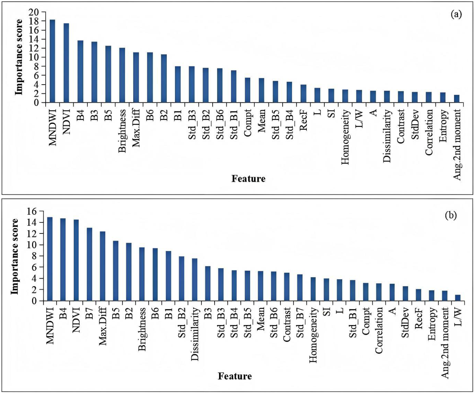
The assessment of feature importance in the TM image (A) and the OLI image (B). For the feature descriptions, please refer to Table 3. The number attached to the abbreviation “B” represents the band order.
2.4.1.4 Optimization of feature selection
Based on the arrangement results, the feature with the highest importance score from the TM image was first selected, followed by the second highest, and so on, forming feature pairs. This process resulted in 29 feature sets, which were progressively added for random forest classification. The classification accuracy for each feature set was then evaluated, and a plot of the relationship between the number of features and classification accuracy was generated (Figure 4A). The results demonstrated that as the number of features increased, the cumulative accuracy initially rose rapidly, but the rate of improvement slowed in the intermediate stages. When the number of features reached 16, the overall accuracy and kappa coefficient peaked at 89.4% and 0.88, respectively. However, as the feature set expanded from 16 to 30, interfeature correlations introduced redundancy, resulting in increased processing time and reduced classifier performance. This led to overfitting, as indicated by a subsequent decrease and fluctuation in classification accuracy. Based on these findings, the top 16 feature combinations were selected as the optimal feature sets for further classification and accuracy assessment. A similar feature optimization process was conducted for the OLI image, resulting in 31 feature pairs. Based on the classification accuracy results (Figure 4B), the top 12 feature combinations were chosen as the final optimal feature set.
Figure 4
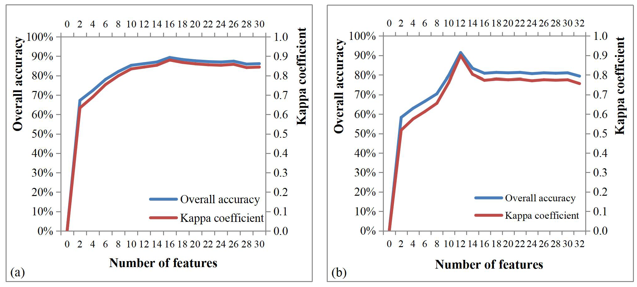
Relationship between the number of features and classification accuracy in the TM image (A) and the OLI image (B).
2.4.1.5 Image classification and accuracy assessment
Wetland type information was extracted from Landsat TM and OLI images, respectively, based on the optimized features. A total of 470 verification points were randomly selected in the whole study area. According to the field survey data, the actual wetland types of the verification points in 2021 were determined. For the other three phases, the actual wetland types of the verification points were determined by integrating historical data, field survey data, and high-resolution imagery. Verification points were used to evaluate each classification result to establish a transition matrix. The overall accuracy and kappa coefficient were calculated using the transition matrix to evaluate the accuracy of the above four classification results (Table 4).
Table 4
| Date | Overall accuracy | Kappa coefficient |
|---|---|---|
| September 15, 1990 | 90.00% | 0.89 |
| September 10, 2000 | 89.36% | 0.88 |
| October 11, 2011 | 88.09% | 0.87 |
| August 19, 2021 | 91.49% | 0.90 |
Classification accuracy evaluation for four periods.
The overall accuracy of the classification results from 1990 to 2021 in Table 4 was more than 88%, and the kappa coefficient was above 0.88, which met the requirements of land cover change monitoring.
2.4.2 Dynamic degree of single wetland type
The dynamic degree model of land use is adopted to reflect the change range of various types of coastal wetlands, and its expression is shown in Equation 1 as follows (Wang and Bao, 1999):
Where K represents the dynamic degree of a wetland type during the study period; Ua and Ub are the areas of a certain wetland at the beginning and the end of the study, respectively; and T is the time interval.
2.4.3 Transition matrix
In order to further analyze the changes of wetlands in the study area, classification results from 1990 to 2021 were used for a spatial superposition analysis to obtain the transition matrix tables of each type. Based on chronological order, the type transition of the YRE coastal wetland from 1990 to 2021 was divided into 1990–2021, 1990–2000, 2000–2011, and 2011–2021.
The Markov transition matrix (Equation 2) refers to the quantitative description of the state and state transition of the studied system (He, 2011), and the wetland transition matrix can quantitatively reveal the mutual transformation between wetland types.
In this formula, p is the area of landscape types; n is the number of coastal wetland landscape types; i and j are the coastal wetland landscape types at the beginning and end of the study; and pij is the area of landscape type j transformed from landscape type i.
2.4.4 Analysis of driving forces for wetland type changes
Based on the research area’s actual conditions and previous studies, we adopted a combined qualitative–quantitative approach to analyze the driving forces behind wetland changes. We selected 14 indicators categorized into two major types—natural factors and socioeconomic factors—that may influence the changes in coastal wetlands at the Yalu River Estuary. Through principal component analysis (PCA) (Mattson et al., 2024), we eliminated redundant indicators and retained 10 key factors. Pearson correlation analysis was then conducted to evaluate the correlation between wetland types and these factors, as fully detailed in Supplementary Document Section S2.
3 Results
3.1 Wetland types and distribution
Shallow marine waters, tidal wetlands, aquaculture ponds, and paddy fields are the predominant wetland types (Figure 5, Table 5), together accounting for 90.03% of the study area in 2021. The first two are natural wetland types, while the latter two are artificial, comprising 66.34% and 23.69%, respectively. These four main wetland types are distributed in bands successively along the coastline, from the sea to the land, forming a stable landscape pattern over the past 31 years. The distribution of reed wetlands is concentrated on both sides of the Dayang River. Other wetland types, including ditches, reservoirs, and salt flats, are fewer in number and dispersed.
Figure 5
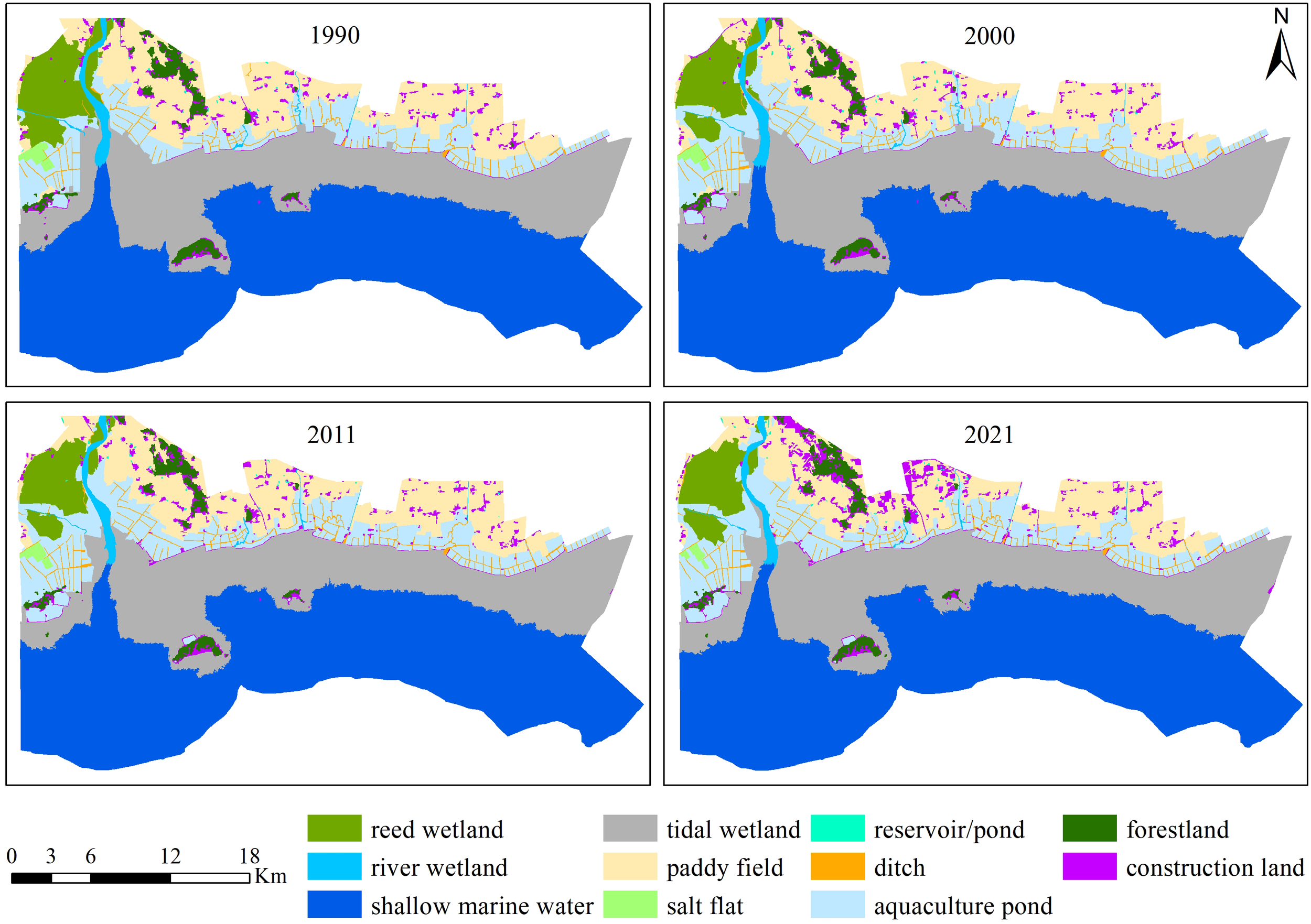
Classification map of the Yalu River coastal wetlands in four periods.
Table 5
| Wetland type | Area/hm2 | Dynamic degree/% | |||||||
|---|---|---|---|---|---|---|---|---|---|
| Year 1990 | Year 2000 | Year 2011 | Year 2021 | 1990–2000 | 2000–2011 | 2011–2021 | 1990–2021 | ||
| Natural wetland | Reed wetland | 3,422.88 | 2,835.81 | 2,665.53 | 2,620.44 | −1.72 | −0.55 | −0.17 | −0.76 |
| River wetland | 803.24 | 791.72 | 741.22 | 723.15 | −0.14 | −0.58 | −0.24 | −0.32 | |
| Shallow marine water | 36,235.44 | 35,966.25 | 35,712.66 | 35,474.76 | −0.07 | −0.06 | −0.07 | −0.07 | |
| Tidal wetland | 20,150.66 | 19,980.01 | 19,739.68 | 19,912.94 | −0.08 | −0.11 | 0.09 | −0.04 | |
| Total area | 60,612.22 | 59,573.79 | 58,859.09 | 58,731.29 | −0.17 | −0.11 | −0.02 | −0.10 | |
| Artificial wetland | Paddy field | 10,960.29 | 10,795.86 | 10,726.37 | 9,734.22 | −0.15 | −0.06 | −0.92 | −0.36 |
| Salt flat | 275.85 | 224.19 | 211.41 | 138.96 | −1.87 | −0.52 | −3.43 | −1.60 | |
| Reservoir/pond | 51.12 | 65.7 | 63.81 | 62.28 | 2.85 | −0.26 | −0.24 | 0.70 | |
| Ditch | 721.98 | 829.99 | 895.87 | 896.04 | 1.50 | 0.72 | 0.00 | 0.78 | |
| Aquaculture pond | 7,971.55 | 9,142.08 | 9,707.13 | 10,044.91 | 1.47 | 0.56 | 0.35 | 0.84 | |
| Total area | 19,980.79 | 21,057.82 | 21,604.59 | 20,876.41 | 0.54 | 0.24 | −0.34 | 0.14 | |
| Non-wetland | Forestland | 1,447.56 | 1,285.92 | 1,275.46 | 1,353.78 | −1.12 | −0.07 | 0.61 | −0.21 |
| Construction land | 1,443.25 | 1,566.29 | 1,744.68 | 2,522.34 | 0.85 | 1.04 | 4.46 | 2.41 | |
Area and dynamic degree of wetland types in the Yalu River coastal wetland from 1990 to 2021.
Note: Bold numbers denote significant transitions between wetland types.
3.2 Areal change
3.2.1 Total area of the wetlands
The area and dynamic degree of wetland types in YRE from 1990 to 2021 are shown in Table 5. From 1990 to 2011, the total area of wetlands remained relatively stable with minor fluctuations. However, from 2011 to 2021, a significant downward trend was observed, with a decrease in the area of 885.98 hm2. The dynamic degree in the total wetlands, from 1990 to 2021, was −0.04%, representing the average annual wetland loss rate in YRE.
3.2.2 Natural wetlands
Natural wetlands experienced a continuous decline of 1,880.93 hm2 over the past 31 years, with an overall dynamic degree of −0.1%. The rate of loss slowed across three periods (from 1990 to 2000, from 2000 to 2011, and from 2011 to 2021), with decreases of −0.17%, −0.11%, and −0.02%, respectively.
Among the various natural wetland types, reed wetlands and shallow marine waters experienced the most significant decreases, losing 802.44 and 760.68 hm², respectively. However, tidal wetlands showed growth from 2011 to 2021 due to wetland restoration efforts, indicating a different trend.
3.2.3 Artificial wetlands
Initially, the artificial wetlands increased significantly from 1990 to 2011, then decreased after 2011, resulting in an overall net increase of 895.62 hm2 and a total dynamic degree of 0.14%. Different types of artificial wetland displayed diverse dynamics. Aquaculture ponds expanded successively by 2,073.36 hm2 over the 31 years, with gradually slower rates of 1.47%, 0.56%, and 0.35%, respectively, across three periods. By 2021, aquaculture ponds accounted for 48.12% of artificial wetlands, covering an area of 10,044.91 hm2. Ditches, which are distributed alongside aquaculture ponds, also showed a simultaneous increasing trend. In contrast, paddy field and salt flats exhibited similar reductions, becoming substantial from 2011 to 2021, with the dynamic degrees up to −0.92% and −3.43%, respectively. By 2021, paddy field had dropped to the second largest artificial wetland type after aquaculture ponds due to a total loss of 1,226.07 hm2.
3.2.4 Non-wetland
It is notable that construction land, a non-wetland type, is widely scattered and distributed, with a significant expansion by 1,079.09 hm2 from 2011 to 2021.
3.3 Wetland transition
The change characteristics of wetland types varied across different study periods, as presented in Table 6, Figures 6, 7; Supplementary Tables S1–S7. In order to reduce visual confusion and improve the overall visualization effect, to focus on significant changes, the threshold of wetland transition change was set as 0.10% of the study area to exclude small wetland type change in Figure 6.
Table 6
| 1990–2021 | Reed wetland | River wetland | Shallow marine water | Tidal wetland | Paddy field | Salt flat | Reservoir pond | Ditch | Aquaculture pond | Forestland | Construction land |
|---|---|---|---|---|---|---|---|---|---|---|---|
| Reed wetland | 2,570.40 | 64.71 | 9.09 | 167.49 | 5.40 | 20.88 | 582.30 | 2.61 | |||
| River wetland | 12.15 | 490.85 | 186.40 | 12.69 | 1.98 | 0.54 | 95.22 | 3.42 | |||
| Shallow marine water | 7.02 | 35,105.13 | 1,123.28 | ||||||||
| Tidal wetland | 144.19 | 368.64 | 18,517.32 | 83.35 | 904.05 | 1.71 | 131.40 | ||||
| Paddy field | 5.40 | 4.23 | 9,012.15 | 45.36 | 14.49 | 698.49 | 76.14 | 1,104.03 | |||
| Salt flat | 138.87 | 2.43 | 134.55 | ||||||||
| Reservoir/pond | 1.17 | 34.38 | 5.31 | 4.14 | 0.09 | 6.03 | |||||
| Ditch | 7.65 | 669.95 | 43.83 | 0.54 | |||||||
| Aquaculture pond | 13.59 | 11.43 | 1.62 | 198.00 | 0.09 | 101.42 | 7,505.99 | 7.47 | 131.93 | ||
| Forestland | 0.27 | 15.30 | 57.51 | 0.27 | 3.51 | 1,214.64 | 156.06 | ||||
| Construction land | 17.73 | 0.45 | 0.99 | 59.94 | 244.35 | 4.23 | 2.70 | 72.82 | 53.73 | 986.31 |
Transition matrix of the Yalu River Estuary wetland types from 1990 to 2021/hm2.
Figure 6
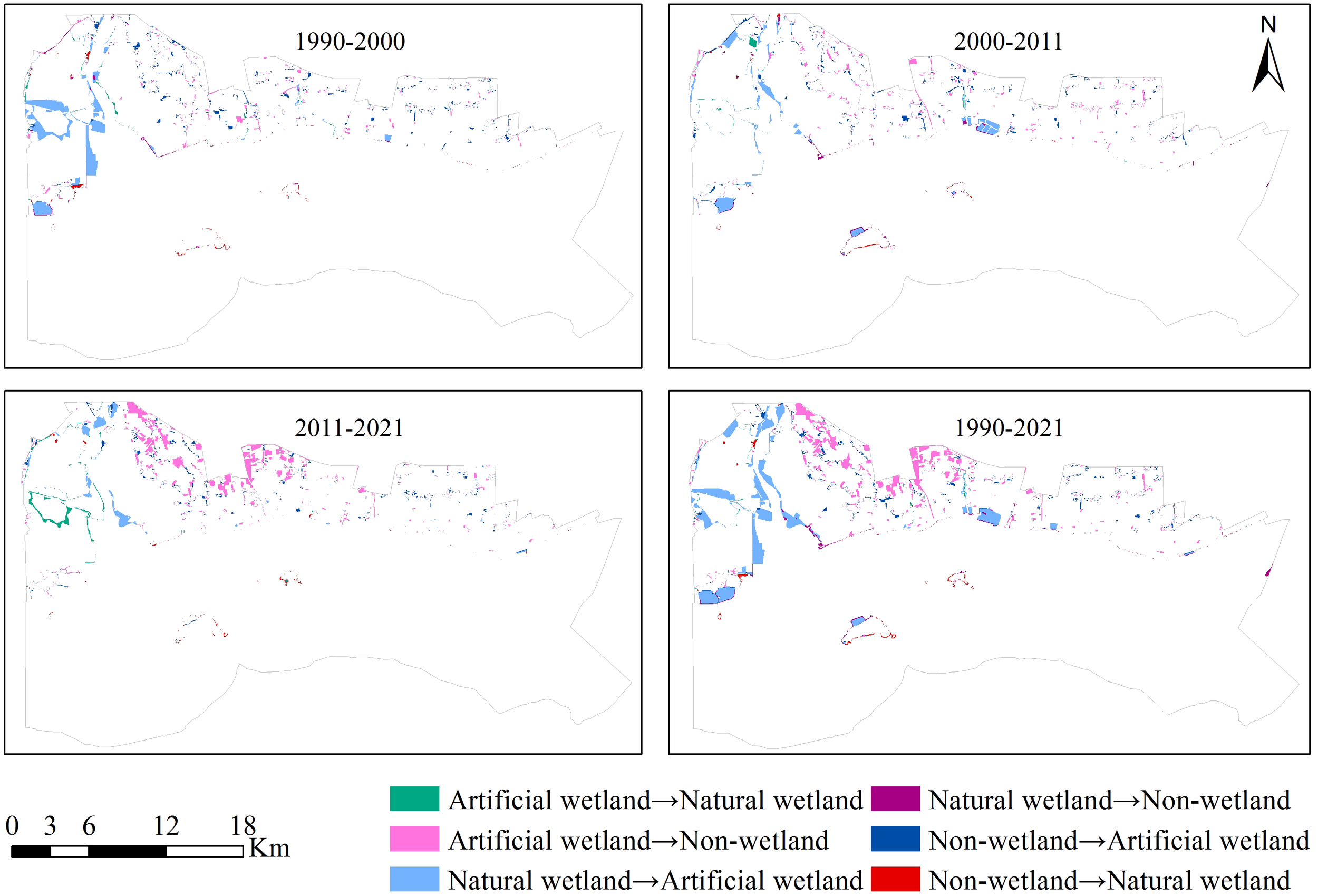
Transition map of the Yalu River Estuary wetlands for four periods.
Figure 7
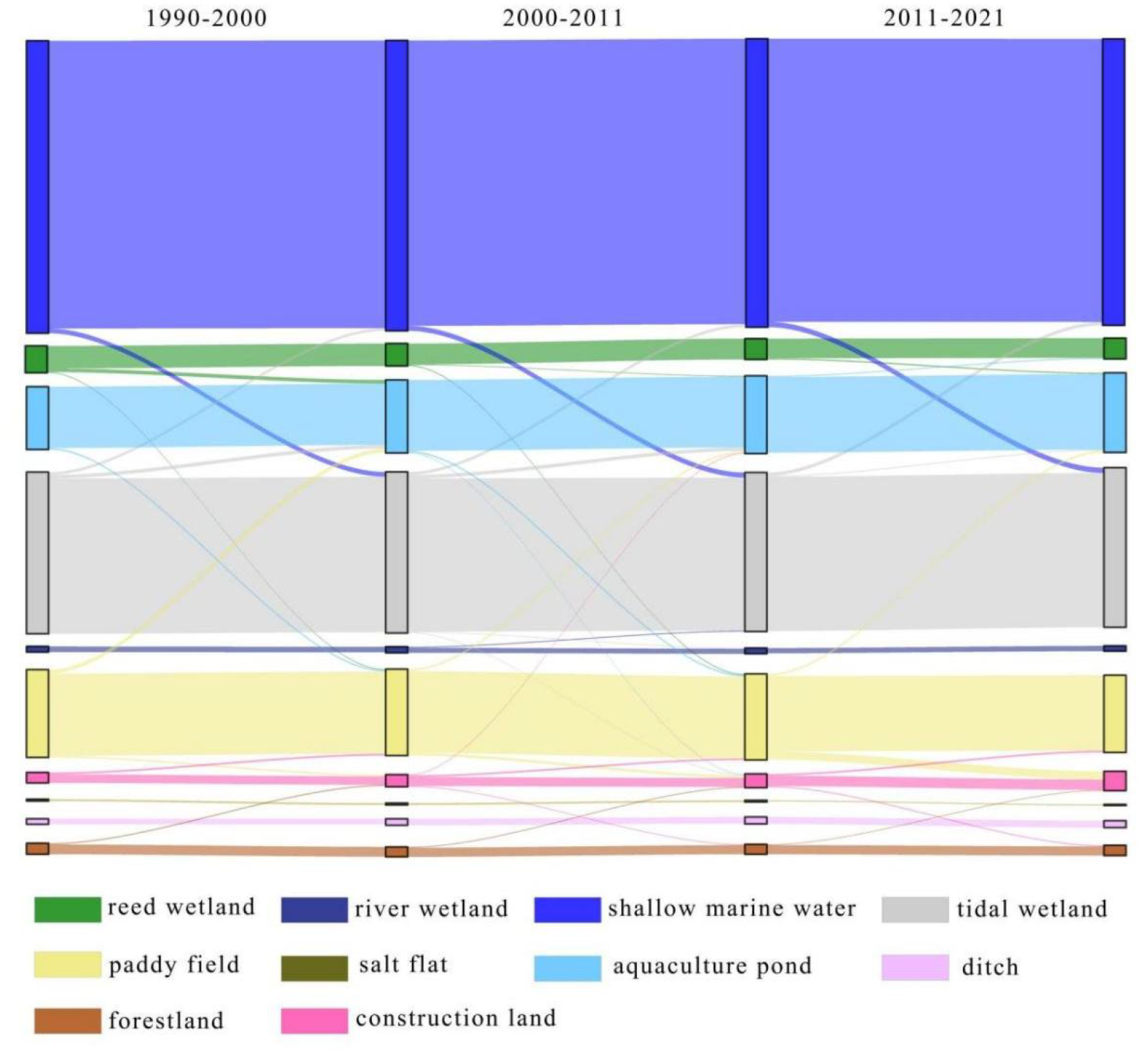
Sankey diagram of different wetland type dynamics in Yalu River Estuary wetland from 1990 to 2021.
3.3.1 Wetland transition from 1990 to 2000
From 1990 to 2000, the transfer-out characteristics of various wetland types were as follows: the maximum transfer-out area came to tidal flats with 913.23 hm2, of which 48.82% was converted to aquaculture ponds and 37.07% to shallow marine waters. Paddy fields and reed wetlands were next, and the transfer-out area was 789.04 and 642.24 hm2, respectively, among which, 61.50% of paddy fields and 70.80% of reed wetlands were converted to aquaculture ponds.
Therefore, aquaculture ponds received the largest transfer-in area at 1,552.51 hm², predominantly from paddy fields, reed wetlands, and tidal wetlands, followed by tidal wetlands and paddy fields, with the transfer-in areas of 742.58 and 624.60 hm2, respectively. The transfer-in area is primarily located in Gushan Town, a key aquaculture region in Dandong City. According to the data from the Dandong Municipal Bureau of Statistics, aquaculture output in the city grew from 41,900 tons in 1990 to 215,000 tons in 2000. As one of the primary industries supporting the local coastal communities, the rapid expansion of aquaculture has played a significant role in driving the conversion into aquaculture ponds in the study area.
3.3.2 Wetland transition from 2000 to 2011
The wetland transition from 2000 to 2011 showed a similar character to the previous 10 years. From 2000 to 2011, tidal wetlands regained the maximum transfer-out area of 1,022.35 hm2, with 42.60% being converted to aquaculture ponds and 36.22% to shallow marine waters. Of the paddy fields transferred out, 48.20% were converted to construction lands, while 35.97% became aquaculture ponds. The transfer-out area of shallow marine waters was 624.78 hm2, with the majority converted into tidal wetlands.
Meanwhile, aquaculture ponds were enlarged with the maximum transfer-in area of 933.33 hm2, mainly transferred from tidal wetlands, paddy fields, and reed wetlands. The transfer-in of tidal wetlands mainly came from shallow marine waters and river wetlands, and that of construction lands mainly came from paddy fields and forestlands. The changes in wetland types during this stage display characteristics and driving factors similar to those observed in the previous period (1990–2000).
3.3.3 Wetland transition from 2011 to 2021
From 2011 to 2021, the maximum transfer-out area was 1,396.42 hm2 of paddy fields, with 72.22% being converted to construction lands and 17.99% to aquaculture ponds. The reciprocal transformation between the shallow marine waters and tidal wetlands dominated the transfer-out of both with 660.87 and 421.09 hm2, respectively. Construction lands received the largest transfer-in area of 1,234.78 hm², primarily from paddy fields.
Unlike the previous two decades, the significant increase in construction land transfer during this period was closely linked to local urbanization and infrastructure development—such as housing and transportation—under the national New Rural Policy. Furthermore, large-scale transitions from artificial to natural wetlands occurred for the first time, in alignment with ecological restoration projects in Dandong City (2018–2021) under the “Blue Bay” Remediation Action. These efforts encompassed coastal wetland restoration, intertidal and shallow marine habitat rehabilitation, nearshore hydrodynamic restoration for islands, island vegetation conservation, and the enhancement of ecological monitoring and early-warning systems within protected areas.
3.3.4 Wetland transition from 1990 to 2021
Over the 31 years, the transition between natural wetlands and artificial wetlands was the most obvious, mainly distributed in the western region of the study area (Figure 6). In the reduced natural wetland area, 1,873.90 hm2 was converted to artificial wetlands, of which 1,581.57 hm2 was converted to aquaculture ponds, 180.18 hm2 was converted to paddy fields, 104.77 hm2 was converted to ditches, and 7.38 hm2 was converted to reservoirs/ponds. However, only 37.44 hm2 of artificial wetlands were converted to natural wetlands. The transition between wetlands and non-wetlands was the second most significant transition observed, mainly distributed in the north of the study area near populated towns. A total area of 1,465.37 hm2 of wetlands was converted into non-wetlands, with forestlands and construction lands receiving 85.41 and 1,379.97 hm2, respectively. There was 480.07 hm2 of non-wetlands converted into wetlands, including paddy fields of 301.86 hm2 and aquaculture ponds of 76.33 hm2, among others.
From 1990 to 2011, a large number of tidal wetlands, paddy fields, and reed wetlands were converted into aquaculture ponds, and the area of aquaculture ponds increased significantly. From 2011 to 2021, the area of paddy fields decreased significantly, and most of them were converted to construction lands. The mutual transfer between shallow marine waters and tidal wetlands was likely related to the hydrodynamic process, the water level of images, or the interpretation cognition. In short, the area of artificial wetlands was increasing, while that of natural wetlands was decreasing.
4 Discussion
4.1 Wetland loss and gain and their forces
Wetland loss has always been the core concern of its protection, i.e., the main threats to migratory shorebirds and residential species. According to historical records, reclamation of natural wetland for paddy field in the YRE dated to the 1950s, and extensive reclamation occurred in the 1980s for paddy field, aqua ponds, roads, and industrial land, giving rise to 30% of the tidal flat lost from the 1960s to the 1980s in sum (Yalu River Estuary Nature Reserve Administration, 1996). The average loss rate from the 1960s to the 1980s is 1% annually, which accords with that in the Yellow Sea from the 1980s to 2010s (Yim et al., 2018). However, in this present study, the natural wetland of YRE decreased at an average rate of 0.10% per year in the past 30 years from 1990 to 2001, among which the proportion of reed, river, tidal flat, and shallow water decreased by 0.96%, 0.10%, 0.28%, and 0.91%, respectively. Overall, the loss of natural wetlands is relatively less and slower over the period, compared with that of the Yellow Sea or other coastal wetlands in China (Yim et al., 2018; Chen et al., 2018; Jiang et al., 2015). The overall stability of natural wetlands benefits from the establishment of a natural reserve, and the implementation of protection measures has played an important role. At the same time, the wetland is relatively far from the densely populated city with high development intensity, and the surrounding villages and towns are also conducive to the protection of the wetland.
Meanwhile, the overall area of artificial wetlands has maintained an upward trend, increasing at an average annual rate of 0.03% over the past 31 years. However, there are differences in the performance of different artificial wetland types. The proportion of salt fields and paddy fields is decreasing, with the lost areas being transformed into non-wetlands, while aquaculture ponds are on the rise continually. Artificial wetlands located near villages and towns were more likely to be converted into houses, roads, and commercial grounds, due to residential area expansion. The artificial wetland area gained by natural wetlands offsets the conversion to non-wetland areas, leading to a net gain in artificial wetlands.
Different from land reclamation resulting in massive wetland loss in other regions in the Yellow Sea (Koh and de Jonge, 2014; Murray et al., 2014; Chen et al., 2019), natural wetland in the YRE diminished by converting to artificial wetland related to the development of agriculture, rural construction, and aquaculture industry. Additionally, a small portion of the tidal flat area was converted into non-wetland, specifically for aquaculture manufacturing infrastructure.
According to the analysis of driving forces for wetland type changes based on principal component analysis and Pearson correlation analysis (Supplementary Materials Section S2), “per capita disposable income of farmers” and “aquatic product output” demonstrated significant correlations with the changes in artificial wetlands (Table 7). Therefore, the development of the local aquaculture industry and living conditions are the primary drivers of the loss of natural wetlands. According to statistical data from Liaoning Provincial Bureau of Statistics (Liaoning Provincial Bureau of Statistics, n.d.), the output of aquaculture in Dandong City increased from 41,900 tons in 1990 to 666,000 tons in 2020, showing a steady growth trend (Figure 8). It is slightly gratifying that the transformation of natural wetlands into artificial wetlands will still retain certain ecological functions (Li et al., 2013; Chen et al., 2018).
Figure 8
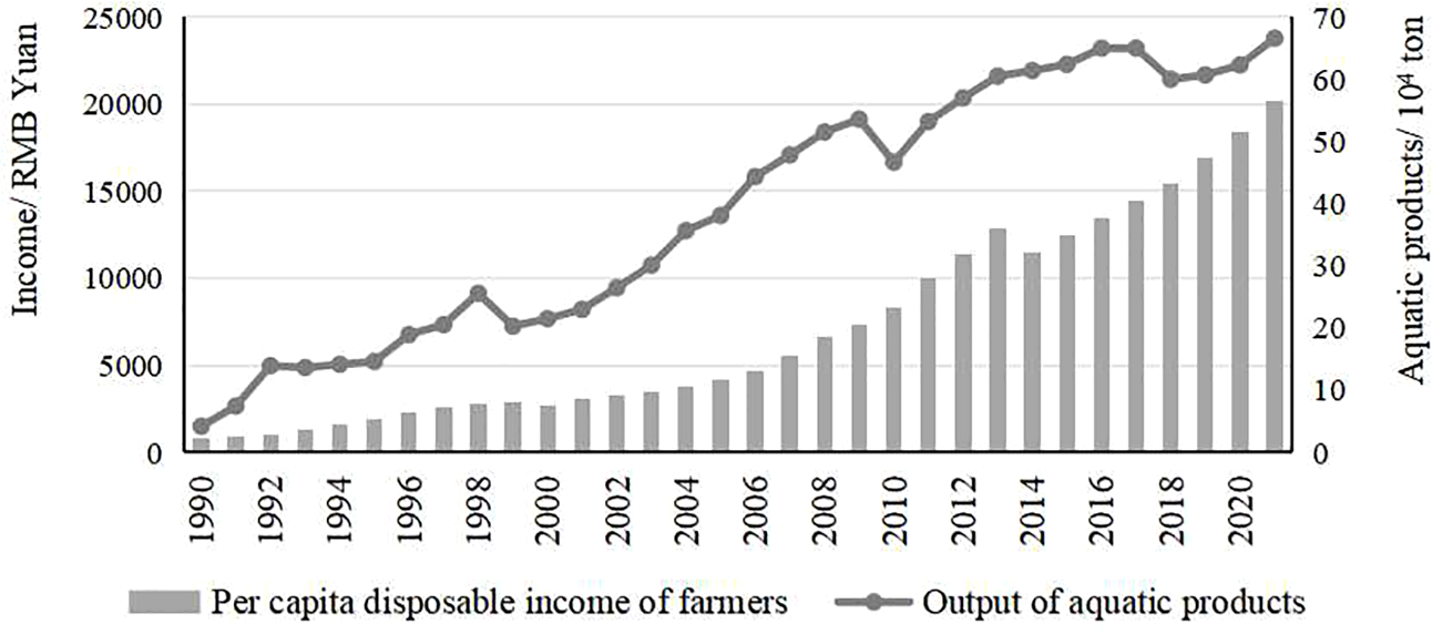
Variation trend of “output of aquatic products” and “per capita disposable income of farmers” from 1990 to 2021 in Dandong City.
Table 7
| Factors | Principal componentsa | Correlation coefficient | |||||
|---|---|---|---|---|---|---|---|
| 1 | 2 | Shallow marine water | Salt flat | Aquaculture pond | Forestland | Construction land | |
| Average annual temperature (X1) | 0.144 | −0.792 | 0.354 | 0.207 | −0.563 | 0.976* | 0.076 |
| Average annual precipitation (X2) | 0.145 | 0.606 | −0.267 | −0.259 | 0.035 | 0.632 | 0.515 |
| Agricultural population (X3) | −0.805 | 0.158 | / | / | / | / | / |
| Natural population growth rate (X4) | −0.872 | 0.117 | / | / | / | / | / |
| Gross regional product (X5) | 0.948 | 0.271 | −0.917 | −0.787 | 0.887 | −0.486 | 0.735 |
| Added value of primary industry (X6) | 0.981 | 0.125 | −0.976* | −0.923 | 0.905 | −0.352 | 0.91 |
| Added value of secondary industry (X7) | 0.777 | 0.503 | / | / | / | / | / |
| Added value of tertiary industry (X8) | 0.987 | 0.066 | −0.976* | −0.925 | 0.902 | −0.342 | 0.915 |
| Local fiscal revenue (X9) | 0.903 | 0.341 | −0.956* | −0.908 | 0.865 | −0.269 | 0.921 |
| Per capita disposable income of farmers (X10) | 0.957 | −0.02 | −0.954* | −0.952* | 0.852 | −0.216 | 0.975* |
| Total retail sales of consumer goods (X11) | 0.915 | −0.057 | −0.894 | −0.748 | 0.876 | −0.518 | 0.685 |
| Aquatic product output (X12) | 0.970 | 0.056 | –0.989* | −0.92 | 0.954* | −0.489 | 0.862 |
| Housing construction area (X13) | 0.913 | 0.261 | −0.811 | −0.633 | 0.805 | −0.522 | 0.566 |
| Total length of urban roads (X14) | 0.799 | 0.322 | / | / | / | / | / |
Factor load matrix of each principal component by PCA and correlation coefficient between wetland types and driving factors in the YRE.
*significant at the 0.05 level (double-tailed). a: Bold numbers denote the main factor loadings per principal component. No significant correlation was shown between other wetland types and each factor.
4.2 Community-based wetland conservation
The establishment of the coastal communities based on paddy fields and pond farming had long stood before that of the Yalu River Wetland Reserve. As the land use rights for the intertidal areas of the nature reserve are held by local communities, the coastal long-traditional residential area was originally incorporated in the functional zoning for the reserve (Wei and Cao, 1997), and the conservation of YRE essentially required the involvement of the local communities. Over the past decades, efforts to promote awareness among communities and residents about wetland ecological functions and the necessity of their protection have successfully increased public awareness and engagement. The communities and stakeholders have played a role in the conservation of coastal wetland system and helped control a low rate of the wetland loss. According to the studies of protection efficiency of 23 national coastal wetland reserves in China in 2011, the Yalu River Wetland Reserve was estimated in excellent condition with higher protection efficiency (Zheng et al., 2012). The authors viewed the picture where dozens of aquaculture workers were harvesting the fishery products in the ponds and where hundreds of waterfowls were roosting leisurely and simultaneously. It intuitively reflects the harmony between man and nature and the effect of community-based coastal wetland protection. However, the community-based conservation still faces challenges: on one hand, the aquaculture industry needs to innovate to a more ecologically friendly industry, avoiding adverse effects on the natural feeding grounds of the waterfowls; on the other hand, financial loss resulting from food provision of migratory bird population should be considered to be compensated. The situation of YRE is typical of many parts of the Yellow Sea, and there is an urgent need to better understand the interrelationships between natural and managed shellfish stocks and shorebird foraging to inform future sustainable management decisions and consensus (IUCN, 2023).
4.3 Adaptive management suggestions
Although the YRE has maintained wetlands as the dominant landscape, there are still issues on its protection and management, and further efforts and actions should be taken into account, including mitigation of climate change and sea rise, more research and monitoring actions, and application of an ecosystem-based approach with consideration of the full array of environmental, economic, and societal impacts of human activities (Elliott et al., 2017). The wetland change characteristics in the core zone of the protected area did not exhibit marked differences from those in the buffer and experimental zones. This suggests that the current functional zoning and management practices may not be fully effective, highlighting the need to optimize the zoning plan and implement differentiated management strategies. Natural wetlands should be prioritized for designation as core protection zones, with conservation efforts focused on preventing their conversion to artificial wetlands and construction land. Cumulative effect assessment shows that the YRE is of high ecological significance with high cumulative risk (Ma et al., 2023); therefore, adaptation management should be undertaken correspondingly. The wetland restoration project has been carried out in the YRE in 2020 to recover natural wetland and solve the hardening problem of the tidal flat. The effect of restoration needs to be monitored and evaluated, and further restoration actions should be undertaken if necessary. Our study offers a methodological framework for long-term and periodic monitoring of coastal wetlands, as well as for evaluating the effectiveness of conservation interventions that could be applied as an adaptive management tool. Furthermore, the Law on Wetland Protection of the PRC came into force in 2022, giving rise to new measures to enhance wetland conservation and fulfilling the commitment of the Ramsar Convention.
5 Conclusion
The study utilized Landsat images to map wetland types and changes in the YRE coastal wetland, providing long-term monitoring datasets from 1990 to 2021. The object-oriented random forest model classification approach was employed and proved to be an effective method for wetland mapping, with overall accuracy ranging from 88.09% to 91.49%. Key findings during the study period included the following: 1) wetland remains the predominant land cover in the study area, with shallow marine waters, tidal wetlands, aquaculture ponds, and paddy fields being the primary wetland types. 2) The most significant changes involved transitions between natural and artificial wetlands. From 1990 to 2011, a substantial amount of tidal wetlands, paddy fields, and reed wetlands were converted into aquaculture ponds, leading to a significant increase in the area of aquaculture ponds. 3) From 2011 to 2021, the area of paddy fields decreased considerably, with many being converted to construction lands.
The YRE coastal wetland has been designated as a nature reserve since 1989 to preserve the coastal wetland ecosystem and protect shorebird populations. Functional zoning was established to regulate land use and control wetland conversion. Despite rapid development in agriculture, rural construction, and the aquaculture industry, the study findings revealed that only 1,880.93 hm² of natural wetland was converted to artificial wetland and construction land over the 31-year period, demonstrating the effectiveness of the reserve’s conservation efforts. However, the significant conversion from artificial wetland to construction land, as well as from natural wetland to artificial wetland, highlights the need for enhanced wetland loss prevention, functional area management and control, and the implementation of restoration projects to recover natural wetland areas from artificial wetlands.
Our study introduces an effective remote sensing framework and provides comprehensive datasets to support long-term and systematic monitoring of coastal wetlands. This framework demonstrates strong potential for future integration with deep learning algorithms to automate the classification and detection of wetland types. Considering the critical importance of sustained and periodic wetland monitoring, future research should further investigate the application of high-resolution and readily accessible remote sensing data, such as Sentinel-2 and synthetic aperture radar (SAR) imagery and integrate these data sources with deep learning techniques, enabling the development of real-time monitoring systems capable of continuously tracking wetland dynamics, thereby providing valuable insights and decision-making support for wetland conservation and management.
Statements
Data availability statement
The original contributions presented in the study are included in the article/Supplementary Material. Further inquiries can be directed to the corresponding author.
Author contributions
JZ: Conceptualization, Investigation, Writing – original draft, Writing – review & editing. XZ: Data curation, Formal Analysis, Writing – original draft. JW: Investigation, Validation, Writing – review & editing. BG: Methodology, Supervision, Writing – review & editing. ZZ: Funding acquisition, Resources, Supervision, Writing – review & editing.
Funding
The author(s) declared that financial support was received for this work and/or its publication. This work was financially supported by the National Natural Science Foundation of China (42376228) and the National Coastal Wetland Monitoring Program of China.
Conflict of interest
The author(s) declared that this work was conducted in the absence of any commercial or financial relationships that could be construed as a potential conflict of interest.
Generative AI statement
The author(s) declared that generative AI was not used in the creation of this manuscript.
Any alternative text (alt text) provided alongside figures in this article has been generated by Frontiers with the support of artificial intelligence and reasonable efforts have been made to ensure accuracy, including review by the authors wherever possible. If you identify any issues, please contact us.
Publisher’s note
All claims expressed in this article are solely those of the authors and do not necessarily represent those of their affiliated organizations, or those of the publisher, the editors and the reviewers. Any product that may be evaluated in this article, or claim that may be made by its manufacturer, is not guaranteed or endorsed by the publisher.
Supplementary material
The Supplementary Material for this article can be found online at: https://www.frontiersin.org/articles/10.3389/fmars.2025.1701014/full#supplementary-material
References
1
Bai Q. Chen J. Chen Z. Dong G. Dong J. Dong W. et al . (2015). Identification of coastal wetlands of international importance for waterbirds: a review of China Coastal Waterbird Surveys 2005-2013. Avian Res.6, 1–16. doi: 10.1186/s40657-015-0021-2
2
Barter M. (2002). Shore birds of the Yellow Sea: Importance, threats and conservation statusGlobal Series 9, International Wader Studies 12 (Canberra, Australia: Wetland International-Oceania: International Wader Study Group), 104. Wetlands International.
3
Barter M. A. Wilson J. R. Li Z. W. Dong Z. G. Cao Y. G. (2000). Yalu Jiang National Nature Reserve, north-eastern China–a newly discovered internationally important Yellow Sea site for northward migrating shorebirds. Stilt37, 13–20.
4
Blaschke T. (2010). Object based image analysis for remote sensing. ISPRS J. Photogrammetry Remote Sens.65, 2–16. doi: 10.1016/j.isprsjprs.2009.06.004
5
Breiman L. (2001). Random forests. Mach. Learn.45, 5–32. doi: 10.1023/A:1010933404324
6
Chen Y. Dong J. Xiao X. Ma Z. Tan K. Melville D. et al . (2019). Effects of reclamation and natural changes on coastal wetlands bordering China’s Yellow Sea from 1984 to 2015. Land degradation Dev.30, 1533–1544. doi: 10.1002/ldr.3322
7
Chen L. Ren C. Zhang B. Li L. Wang Z. Song K. (2018). Spatiotemporal dynamics of coastal wetlands and reclamation in the Yangtze estuary during past 50 years, (1960s–2015). Chin. Geographical Sci.28, 374–385. doi: 10.1007/s11769-017-0925-3
8
Choi C. Y. Battley P. F. Potter M. A. Rogers K. G. Ma Z. (2015). The importance of Yalu Jiang coastal wetland in the north Yellow Sea to Bar-tailed Godwits Limosa lapponica and Great Knots Calidris tenuirostris during northward migration. Bird Conserv. Int.25, 53–70. doi: 10.1017/S0959270914000124
9
Davidson N. C. (2014). How much wetland has the world lost? Long-term and recent trends in global wetland area. Mar. Freshw. Res.65, 934–941. doi: 10.1071/MF14173
10
Elliott M. Burdon D. Atkins J. P. Borja A. Cormier R. De Jonge V. N. et al . (2017). And DPSIR begat DAPSI (W) R (M)!”-a unifying framework for marine environmental management. Mar. pollut. Bull.118, 27–40. doi: 10.1016/j.marpolbul.2017.03.049
11
Granger J. E. Mahdianpari M. Puestow T. Warren S. Mohammadimanesh F. Salehi B. et al . (2021). Object-based random forest wetland mapping in Conne River, Newfoundland, Canada. J. Appl. Remote Sensing.15, 038506. doi: 10.1117/1.JRS.15.038506
12
Guo Y. Wang R. Wang S. (2014). Analysis on the changes in the coastal wetland reserve landscape of Yalu River Mouth. Agric. Sci. Technol. Equip., 6–8.
13
He C. (2011). The Research of Markov Model Porecasing Method and Application (Hefei: Anhui University).
14
He T. Xie J. Xu Y. (2009). Dynamic evolvement of seaside wetland landscape pattern arund the Yalujiang river delta. Acta Scientiarum Naturalium Universitatis Sunyatseni48, 113–118.
15
Hua N. (2014). Fuel deposition of shorebirds at stopping sites in the Yellow Sea during spring migration (Shanghai: Fudan University).
16
Hua N. Tan K. Chen Y. Ma Z. (2015). Key research issues concerning the conservation of migratory shorebirds in the Yellow Sea region. Bird Conserv. Int.25, 38–52. doi: 10.1017/S0959270914000380
17
IUCN (2023). The 2023 IUCN Situation analysis on ecosystems of the Yellow Sea with particular reference to intertidal and associated coastal habitats (Bangkok, Thailand: IUCN).
18
Jiang T. Pan J. Pu X. Wang B. Pan J. (2015). Current status of coastal wetlands in China: Degradation, restoration, and future management. Estuarine Coast. Shelf Sci.164, 265–275. doi: 10.1016/j.ecss.2015.07.046
19
Kashaigili J. J. Mbilinyi B. P. Mccartney M. Mwanuzi F. L. (2006). Dynamics of Usangu plains wetlands: Use of remote sensing and GIS as management decision tools. Phys. Chem. Earth Parts a/B/C31, 967–975. doi: 10.1016/j.pce.2006.08.007
20
Koh C. H. de Jonge V. N. (2014). Stopping the disastrous embankments of coastal wetlands by implementing effective management principles: Yellow Sea and Korea compared to the European Wadden Sea. Ocean Coast. Manage.102, 604–621. doi: 10.1016/j.ocecoaman.2014.11.001
21
Li D. Chen S. Lloyd H. U. W. Zhu S. Shan K. A. I. Zhang Z. (2013). The importance of artificial habitats to migratory waterbirds within a natural/artificial wetland mosaic, Yellow River Delta, China. Bird Conserv. Int.23, 184–198. doi: 10.1017/S0959270913000099
22
Liaoning Provincial Bureau of Statistics . Liao Statistic Yearbook online dataset. Available online at: https://tjj.ln.gov.cn/tjj/tjsj/index.shtml. (Accessed May 20,2022)
23
Lu J. (1990). China Wetland (Shanghai: East China Normal University Press), 25–36.
24
Ma Z. J. Bai Q. Q. Wu W. Feng X. S. Tang C. D. (2013). Differentiating between stopover and staging sites: functions of the southern and northern Yellow Sea for long-distance migratory shorebirds. J. Avian Biol.44, 504–512. doi: 10.1111/j.1600-048X.2013.00213.x
25
Ma L. Li M. Ma X. Cheng L. Du P. Liu Y. (2017). A review of supervised object-based land-cover image classification. ISPRS J. Photogrammetry Remote Sens.130, 277–293. doi: 10.1016/j.isprsjprs.2017.06.001
26
Ma C. Stelzenmüller V. Rehren J. Yu J. Zhang Z. Zheng H. et al . (2023). A risk-based approach to cumulative effects assessment for large marine ecosystems to support transboundary marine spatial planning: A case study of the yellow sea. J. Environ. Manage.342, 118165. doi: 10.1016/j.jenvman.2023.118165
27
MacKinnon J. Verkuil Y. I. Murray N. (2012). IUCN situation analysis on East and Southeast Asian intertidal habitats, with particular reference to the Yellow Sea (including Bohai Sea)Occasional Paper of the IUCN Species Survival Commission No.47 (Gland, Switzerland and Cambridge, UK: IUCN).
28
Mattson M. Sousa D. Quandt A. Ganster P. Biggs T. (2024). Mapping multi-decadal wetland loss: Comparative analysis of linear and nonlinear spatiotemporal characterization. Remote Sens. Environ.302, 113969. doi: 10.1016/j.rse.2023.113969
29
Murray N. J. Clemens R. S. Phinn S. R. Possingham H. P. Fuller R. A. (2014). Tracking the rapid loss of tidal wetlands in the Yellow Sea. Front. Ecol. Environ.12, 267–272. doi: 10.1890/130260
30
Sun Y. (2016). Study on Wetland Information Extraction from Multi-sourced Remote Sensing Imagery and Its Scale Effects Using OBIA Method (Lanzhou: Lanzhou University).
31
Sun Z. Sun W. Tong C. Zeng C. Yu X. Mou X. (2015). China’s coastal wetlands: Conservation history, implementation efforts, existing issues and strategies for future improvement. Environ. Int.79, 25–41. doi: 10.1016/j.envint.2015.02.017
32
Wang X. Bao Y. (1999). Study on the method of land use dynamic change research. Prog. Geogr.18, 81–87. doi: 10.3969/j.issn.1007-6301.1999.01.012
33
Wang Q. Ma Y. Cheng Z. Du Y. (2023). Coastline changes under natural and anthropogenic drivers in a macro-tidal estuary between 2000-2020. Front. Mar. Science.10. doi: 10.3389/fmars.2023.1335064
34
Wang X. Xiao X. Zou Z. Hou L. Qin Y. Dong J. et al . (2020). Mapping coastal wetlands of China using time series Landsat images in 2018 and Google Earth Engine. ISPRS J. Photogrammetry Remote Sens.163, 312–326. doi: 10.1016/j.isprsjprs.2020.03.014
35
Wei C. Cao R. (1997). Functional zoning and conservation strategy of Yalu River Eustuary Coastal Wetland Nature Reserve. Liaoning Urban Rural Environ. Sci. Technol.5, 39–41.
36
Whyte A. Ferentinos K. P. Petropoulos G. P. (2018). A new synergistic approach for monitoring wetlands using Sentinels -1 and 2 data with object-based machine learning algorithms. Environ. Model. Software104, 40–54. doi: 10.1016/j.envsoft.2018.01.023
37
Wu T. Zhang G. Yan J. Cai Y. Fang H. Sun J. et al . (2021). Dynamic evolution of landscape pattern and its driving forces in Yalujiang delta coastal wetland during the last 30 years. Mar. Environ. Sci.40, 683–690.
38
Xu Y. Shao J. Yang W. Wang W. Cui Y. Song Q. (2006). Research on classification and change of seaside wetland around Yalujiang river estuary based on RS and GIS. Geoscience, 500–503. doi: 10.3969/j.issn.1000-8527.2006.03.020
39
Yalu River Estuary Nature Reserve Administration (1996). Survey report of the Yalu river estuary nature reserve.
40
Yang X. C. Zhu Z. Qiu S. Kroeger D. K. Zhu Z. L. Covington S. (2022). Detection and characterization of coastal tidal wetland change in the northeastern US using Landsat time series. Remote Sens. Environ.276, 113047. doi: 10.1016/j.rse.2022.113047
41
Yim J. Kwon B. O. Nam J. Hwang J. H. Choi K. Khim J. S. (2018). Analysis of forty years long changes in coastal land use and land cover of the Yellow Sea: The gains or losses in ecosystem services. Environ. pollut.241, 74–84. doi: 10.1016/j.envpol.2018.05.058
42
Zekarias T. Govindu V. Kebede Y. Gelaw A. (2021). Geospatial analysis of wetland dynamics on Lake Abaya-Chamo, the main rift valley of Ethiopia. Heliyon7, 1–10. doi: 10.1016/j.heliyon.2021.e07943
43
Zhang C. P. Liu J. W. Yan C. (2014). Change of landscape pattern in Yalu-river estuary wetland. Advanced Materials Res.955, 4057–4060. doi: 10.4028/www.scientific.net/AMR.955-959.4057
44
Zhao H. Wang L. (2000). Classification of the coastal wetland in China. Mar. Sci. Bull.19, 72–82.
45
Zheng Y. Zhang H. Niu Z. Gong P. (2012). Protection effificacy of national wetland reserves in China. China Sci. Bull.57, 1116–1134. doi: 10.1007/s11434-011-4942-9
46
Zhou R. Yang C. Li E. Cai X. Yang J. Xia Y. (2021). Object-based wetland vegetation classification using multi-feature selection of unoccupied aerial vehicle RGB imagery. Remote Sens.13, 4910. doi: 10.3390/rs13234910
Summary
Keywords
dynamic change, object-oriented, random forest model, wetland gain and loss, Yalu River Estuary coastal wetland
Citation
Zhao J, Zhang X, Wang J, Guo B and Zhang Z (2026) Monitoring dynamics of the Yalu River Estuary coastal wetland from 1990 to 2021 through the remote sensing approach. Front. Mar. Sci. 12:1701014. doi: 10.3389/fmars.2025.1701014
Received
08 September 2025
Revised
08 December 2025
Accepted
17 December 2025
Published
14 January 2026
Volume
12 - 2025
Edited by
Vitor H. Paiva, University of Coimbra, Portugal
Reviewed by
Lina Ke, Liaoning Normal University, China
Tao Zou, Chinese Academy of Sciences (CAS), China
Updates
Copyright
© 2026 Zhao, Zhang, Wang, Guo and Zhang.
This is an open-access article distributed under the terms of the Creative Commons Attribution License (CC BY). The use, distribution or reproduction in other forums is permitted, provided the original author(s) and the copyright owner(s) are credited and that the original publication in this journal is cited, in accordance with accepted academic practice. No use, distribution or reproduction is permitted which does not comply with these terms.
*Correspondence: Jinxia Zhao, zjx@fio.org.cn
Disclaimer
All claims expressed in this article are solely those of the authors and do not necessarily represent those of their affiliated organizations, or those of the publisher, the editors and the reviewers. Any product that may be evaluated in this article or claim that may be made by its manufacturer is not guaranteed or endorsed by the publisher.