 Baekjin Kim
 Seonghyeon Kim
 Soonyeol Kwon
 Sunjong Lee
 Eung Kim
- 1Sea Power Reinforcement· Security Researcher Department, Korea Institute of Ocean Science and Technology (KIOST), Busan, Republic of Korea
- 2Vessel Observation Team, Korea Institute of Ocean Science and Technology (KIOST), Geoje, Republic of Korea
Introduction: Using May–November 2022 CTD observations from the central–eastern southern coastal waters of Korea, we quantified the variability of oceanic fronts and their coupling with water-column stability.
Methods: We used conventional , thresholds and a composite Integrated Frontal Index (IFI) of , , and N²; the stability effect is - .
Results: Fronts were coherently organized along the coastal–offshore boundary zones near the 70–100 m isobaths. Their intensity and principal formation depths reflected seasonal stratification and thermocline–halocline alignment (ΔTHD ): fronts were sharp and continuous when the clines co-occurred in summer, but diffuse and deeper when offset during autumnal cooling and mixing. Quantitatively, in the upper layer (10–30 m) the IFI closely co-locates with salinity fronts (≈99–100%) and also with temperature fronts (~87–93%), whereas agreement declines and becomes more variable below about 40–50 m. ΔIFI exhibited a depth-dependent pattern (mean −5.7 at 10 m, −1.3 at 60 m, −4.6 at 80 m), consistent with surface weakening, mid-layer mitigation, and renewed deep weakening.
Discussion: The framework captures transitions between salinity- and temperature-dominated regimes and quantifies the amplification–weakening mechanism associated with ΔTHD , providing an observation-based diagnostic for front–stratification coupling.
1 Introduction
An oceanic front is a dynamic boundary characterized by rapid horizontal gradients in seawater properties such as temperature, salinity, and density. Within these frontal zones, various dynamic features exist, including turbulent mixing, internal waves, transport boundaries, biogeochemical boundaries, and sound-speed discontinuities. Frontal zones function as a key spatial element driving the structural heterogeneity of the ocean (Belkin et al., 2010). In particular, fronts within the coastal zone vary in location and intensity due to factors including seasonal variations, inflows of open-ocean water, tides, and topography, significantly altering the water column structure and mixing conditions of the coastal zone.
Oceanic water column stability is defined by vertical and horizontal variations in the density structure of seawater, which is determined by temperature and salinity. Water column stability exerts a crucial influence on oceanic dynamic processes, including mixing, energy transfer, internal wave generation, and shear current formation (Gill, 1982; Thorpe, 2005). In general, highly stable, stratified seawater layers exhibit resistance to external forcing and limit the exchange of material and energy between layers. Conversely, low or negative stability induces turbulence, resulting in enhanced mixing (Pelegrí et al., 2024). Frontal zones are often associated with strong vertical stratification, and vertical stability plays a crucial role in physical processes such as energy transport, vertical mixing, and upwelling within fronts. Therefore, consideration of both the horizontal characteristics and vertical stability of fronts is essential to elucidating frontal dynamics.
Studies on frontal identification have focused mostly on analyzing individual phenomena, such as thermal or tidal fronts, or observational cases of specific time periods or cross-sections. In contrast, comprehensive, three-dimensional, spatiotemporally integrated analyses based on multi-point grid systems and the analysis of dynamic stability indicators have been relatively scarce. Furthermore, conventional criteria for frontal identification have relied primarily on fixed gradient thresholds of temperature and salinity (Table 1) or fixed thresholds (Kawai, 1972; Lynn, 1986; Hickox et al., 2000; Kim et al., 2023; Shin et al., 2024). However, such single-variable approaches have limitations in the comprehensive representation of both frontal intensity and vertical stability. In particular, fully capturing the multidimensional characteristics of fronts formed by the complex interaction of multiple variables, such as density compensation fronts, is challenging. Furthermore, the application of a fixed threshold may lead to subjectivity and discontinuity in detection results due to the lack of adaptation to different frontal types, regions, and seasons.
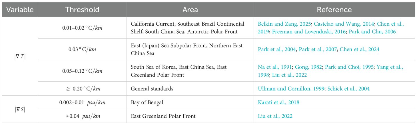
Table 1. Threshold values of horizontal temperature and salinity gradients for frontal identification reported in previous studies of global and regional seas.
Accordingly, the objectives of this study were to quantify the spatiotemporal variations of fronts in the study area using observational data; introduce and apply the Integrated Frontal Index (IFI), which integrates horizontal gradients of temperature and salinity with water column stability; and evaluate the validity of the IFI based on spatial agreement with conventional (threshold-based) fronts. Furthermore, quantification of front–stratification coupling suggests potential applications in operational fields such as marine situational awareness and forecasting of coastal acoustic environments. Ultimately, we aimed to elucidate the spatiotemporal variability characteristics of the front in the study area and its relationship with water column stability, thereby providing an in-depth assessment of frontal dynamics in complex coastal environments.
2 Materials and methods
2.1 Study area and data
This study was conducted in the central-eastern region of the southern coastal waters of Korea (127°E–130°E, 32.75°N–35.5°N). This area is connected to the Yellow Sea through Jeju Strait to the west, to the East Sea (Sea of Japan) through Korea Strait to the east, and to the East China Sea across the continental shelf to the south. The study area is characterized by a dynamic marine environment influenced simultaneously by complex topography, the inflow of the Tsushima Warm Current, seasonal freshwater discharge, and strong tidal forcing. In particular, during summer, the seasonal inflow of low-salinity water from the Yellow Sea and warm surface water leads to enhanced interactions among water masses, resulting in the development of pronounced stratification and seasonal fronts. These complex physical factors drive the formation of strong stratification and diverse fronts within the region, causing horizontal and vertical stability structures to undergo rapid seasonal variations.
Field observations were conducted four times at 2-month intervals from May to November 2022. The marine environmental survey was conducted using the Korea Institute of Ocean Science and Technology (KIOST) research vessels ‘R/V Onnuri’ and ‘R/V Ieodo’. The observation array consisted of 130 stations along 16 transects (Figure 1). At each station, vertical profiles of seawater properties were obtained using conductivity–temperature–depth (CTD; SBE 911plus, Sea-Bird Electronics, Bellevue, WA, USA) instruments. CTD data were calibrated and outliers removed, and the data were bin-averaged at 1-m depth intervals. Profiles were objectively mapped using optimal interpolation (OI) onto a 215 × 195 grid (0.015 km spacing) with an isotropic Gaussian covariance. Following Bretherton et al. (1976), we computed OI weights and the analysis-error variance and report its square root at each grid point as an interpolation-uncertainty diagnostic. Horizontal gradients (, ) were then computed on the km-scaled grid using centered differences. Because the covariance correlation length exceeds the 0.015 km spacing, neighboring cells are not independent. To ensure spatial consistency and interpretive reliability, we restricted analyses to a common depth range down to 80 m. This criterion was adopted because major physical variations such as stratification, mixing, and frontal formation are generally concentrated within the upper 80 m in the study area. Deeper data were deemed unsuitable for horizontal–vertical comparisons and statistical analyses due to depth differences among stations and structural inhomogeneity.
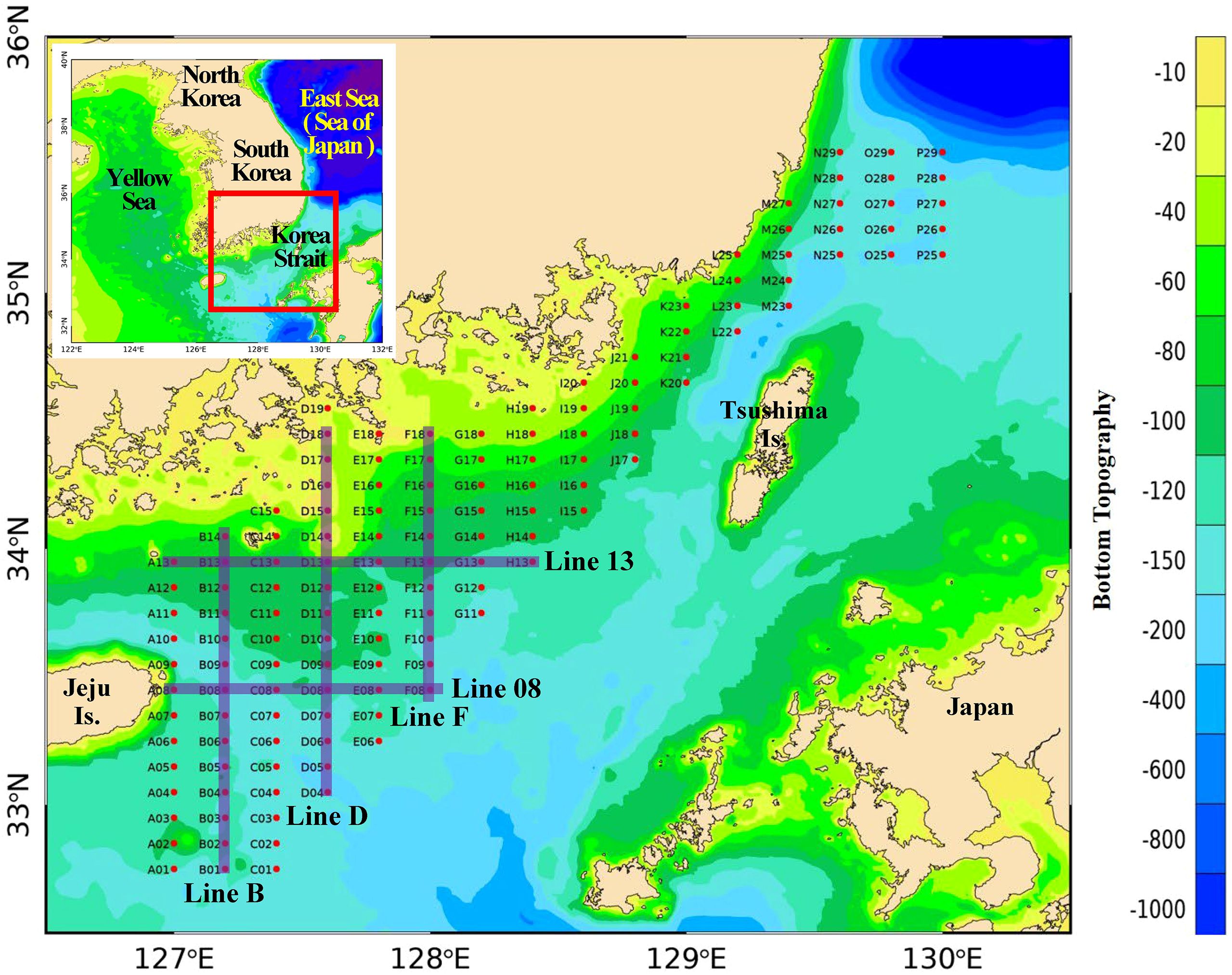
Figure 1. Map of the study area and CTD observation array. In total, 130 CTD stations were arranged along 16 transects across the central-eastern part of the southern coastal waters of Korea.
2.2 Methodology of front and stability index derivation
To quantitatively assess the characteristics of fronts in the study area, stratification and stability indices were calculated. Each index was derived from the spatial structures of temperature, salinity, density, and the indices were used to comprehensively diagnose the physical stability of the ocean.
2.2.1 Calculation of stability indices and vertical stratification
The Brunt–Väisälä Frequency (N²; Gill, 1982) is an indicator of stratification stability calculated from the vertical gradient of the density field derived from temperature and salinity, defined as follows:
where is gravitational acceleration, is the reference density, and represents the vertical density gradient. This index indicates the degree of buoyant stability within the water column, where positive values represent stable stratification and negative values indicate density inversion or unstable conditions. In this study, we calculated the N² value for each water layer and the average N² value across all layers to analyze seasonal variations in stability.
To quantify the vertical stratification structure of the sea area, the thermocline depth (TD) and halocline depth (HD) were defined as the depths at which the maximum vertical gradient occurs for temperature and salinity, respectively. These values represent the depths where thermal and haline stratification are most strongly developed. The difference between the two depths, expressed as ΔTHD (TD − HD), was used as an index to diagnose the asymmetry of thermal and haline stratification. TD and HD were estimated based on the following relations:
Here, and represent the vertical gradients of temperature and salinity, respectively, calculated using the central difference scheme based on interpolated temperature and salinity profiles at 1-m intervals. ΔTHD is defined as follows:
A positive value of ΔTHD indicates the relative dominance of salinity-driven stratification, whereas a negative value suggests the predominance of thermal stratification or the potential intrusion of high-salinity water into the upper layer. Smaller absolute values of ΔTHD indicate that the two clines are collocated at similar depths, and thus efficiently increase density stratification. Conversely, a larger absolute value increases the likelihood of weakened density stratification due to compensation effects from thermal and haline gradients. This indicator was used to diagnose the presence of double stratification and vertical asymmetry of fronts and provided a key basis for interpreting the relationship between fronts and stability.
2.2.2 Thresholds for traditional frontal identification
Traditional methods of oceanic front identification primarily define fronts as regions where the horizontal gradient of temperature or salinity exceeds a specific threshold. However, such thresholds have been proposed with considerable variation depending on the type of front, geographic location, season, and research objectives. To ensure reproducibility in the definition of fronts, thresholds reported in previous studies were compiled by variable and category (Table 1). Guided by these literature ranges and by the resolution and noise characteristics of our gridded fields, we adopted conservative baseline thresholds appropriate for continental-shelf settings and within reported ranges:
These thresholds were used to define the conventional front masks for comparisons with IFI‐based fronts.
2.2.3 Integrated frontal index determination and comparative analysis
The IFI is computed as a weighted sum of , , and N² after applying ) and per-depth 0–1 normalization. The logarithm is a monotonic variance-stabilizing transform for heavy-tailed horizontal gradients: it limits the dominance of a few extreme frontal cores while preserving rank ordering, so cores remain in the upper tail under our percentile masks.
To characterize the front-stability relationship, we define two indices:
Here, denotes per-depth 0–1 normalization. All weights and were derived from the first principal component (PC1) loading of principal component analysis (PCA) (Thomson and Emery, 2014; Jolliffe and Cadima, 2016; Wolter and Timlin, 2011) and were normalized such that .
PCA loadings provide a pragmatic, data-adaptive weighting, but they maximize variance rather than dynamical importance and can overweight salinity in freshwater-dominated seasons. As a physics-based alternative, the and weights are set in proportion to their density-gradient contributions via the thermal-expansion and haline-contraction coefficients (α and β). we take layer-wise weights proportional to and and then normalize. A brief sensitivity check using these α–β layer weights is given in Supplementary Table S3 as depth-dependent bilateral spatial agreement with the PCA-weighted . Thresholding and spatial-agreement definitions follow below.
We retain the conventional definition of a front via and , and use IFI as an integrative diagnostic of front–stratification coupling. The stratification term (N²) is not used to define a front but to quantify its context. IFI is a composite diagnostic of the front–stratification state. Front presence and footprint are diagnosed by , , whereas N² does not define a front but supplies the stratification context that modulates its intensity, vertical extent, and preferred formation depth. After consistent scaling, we combine , , and N2 to summarize the co-occurrence and coupling of horizontal frontal gradients with vertical stability, preserving the conventional front definition while explicitly accounting for stratification across depths and seasons.
The conventional front mask is defined as follows:
The IFI front mask was defined as follows based on the top-15% threshold:
The agreement between conventional fronts (A, B) and IFI fronts ( or ) is quantified as spatial agreement (hereafter reported as coverage), defined as the overlap percentage. To evaluate the explanatory capacity of front–stratification coupling, we fix the IFI fronts as the reference set C unless noted otherwise, and compute:
Here, C denotes the IFI mask used in the comparison ( or ) and represents the total number of valid grid points. Note that is asymmetric. It measures the fraction of X explained by Y. All values are reported in percent.
We adopt a depth-wise (per-depth) percentile rule because it is unitless and amplitude-invariant, allowing the monotonic, per-depth–scaled fields to target the upper tail consistently across depths and seasons. In practice, a 15% cutoff provides a pragmatic balance between excessive patchiness at lower percentiles and over-identification of background at higher ones; varying the percentile between 10–20% does not alter our qualitative conclusions (see Section 3.3.1).
3 Results
In this section, the physical background of the study area is first presented. Then, based on the indicators defined in Section 2, the spatiotemporal distributions of stratification and stability indicators are analyzed, and the structural characteristics and seasonal variability of fronts are examined.
3.1 Characteristics of the marine physical environment
3.1.1 Distributions of temperature and salinity
The distributions of temperature and salinity in the study area, obtained from four observations conducted between May and November 2022, exhibited distinct spatial variations with depth and season. During the entire period, temperature ranged from 3.4 to 26.9°C. The mean temperature at a depth of 10 m was 21.3°C, and at 80 m it was 16.6°C. The standard deviation decreased with depth, from 3.3°C to 2.5°C (Supplementary Table S1). The horizontal distribution showed a seasonal increase throughout the study area from May to September, followed by a decrease in November (Figure 2; Supplementary Figure S1A). By region, the northeastern parts of Jeju Island (127–128°E, north of 33.5°N) maintained lower surface temperatures than surrounding areas from May to September, with a thin warm layer observed in the upper water column (0–30 m) (Supplementary Figure S1A). In the southeastern parts of Jeju Island (127–128°E, south of 33.5°N), a warm temperature belt was widely distributed during the same period, with a distinct pattern of expansion to depths of 30–50 m in July and September. The eastern part of the southern coastal waters (128–129°E) showed a year-round trend of lower temperature on the coastal side compared to the offshore side. When a warm layer formed in the upper water column during summer, it was relatively shallow and weak on the coastal side (Figure 2A).
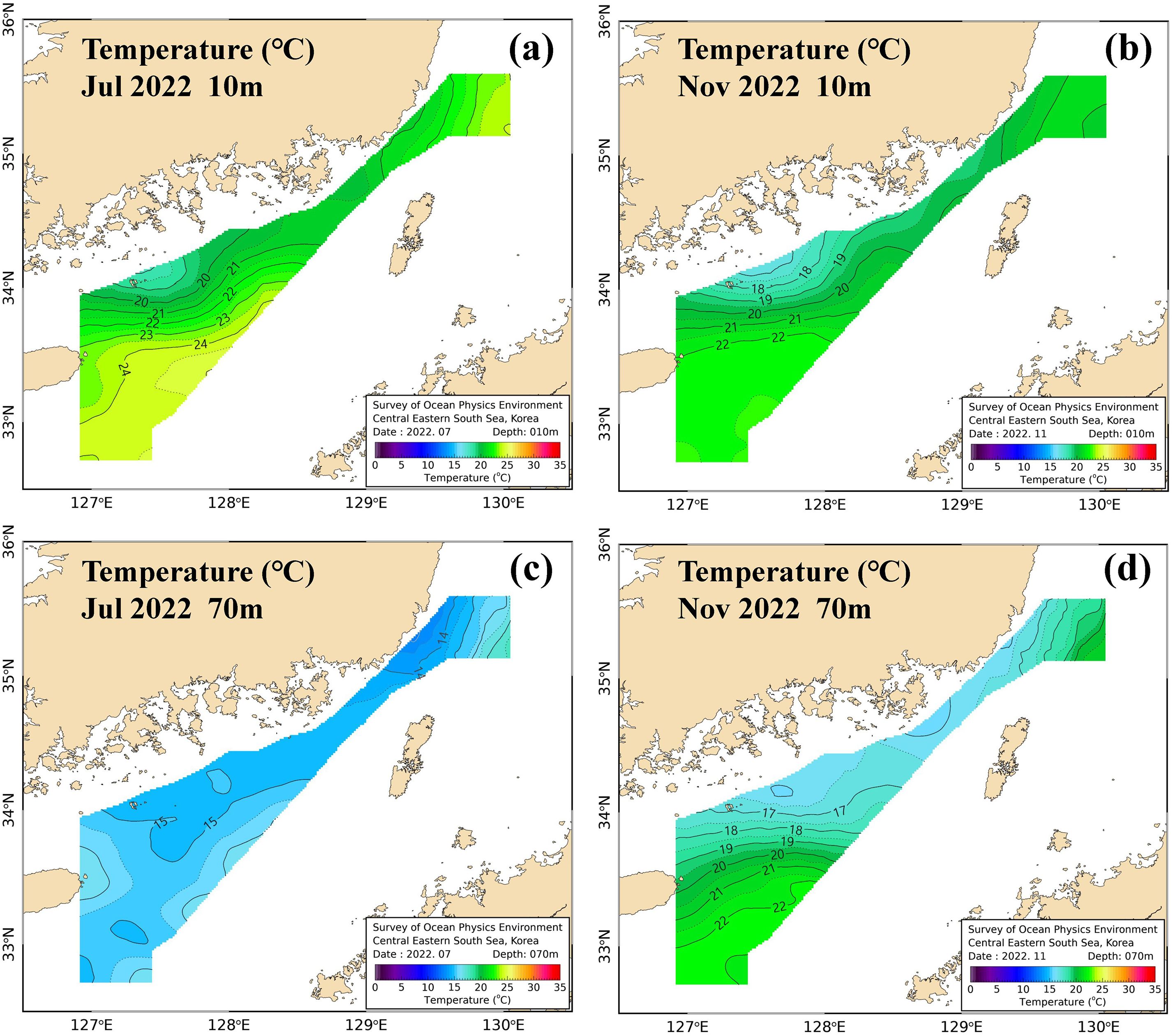
Figure 2. Horizontal distributions of temperature at 10 m and 70 m in July and November 2022: (a) July at 10 m, (b) November at 10 m, (c) July at 70 m, and (d) November at 70 m.
Salinity ranged from 31.2 to 34.7 psu, with mean salinity of 33.5 psu at 10 m and 34.3 psu at 80 m. The standard deviation decreased with depth, from 0.7 to 0.2 psu (Supplementary Table S1). Seasonal variation was observed, with low-salinity zones along the coast expanding during July–September and contracting in November (Figure 3; Supplementary Figure S1B). In the northeastern waters of Jeju Island, low-salinity patches appeared and persisted from summer to early autumn, with a relatively low-salinity layer observed down to 30 m (Supplementary Figure S1B). The southeastern waters of Jeju Island exhibited a dominant high-salinity distribution throughout the study period, with a stable high-salinity zone appearing below 30 m. The eastern part of the southern coastal waters exhibited a recurring pattern of a low-salinity layer expanding in a band-shaped formation from July to September before contracting in November, with vertical contrast between low salinity in the upper layer and high salinity in the deeper layer (Figure 3; Supplementary Figure S1B).
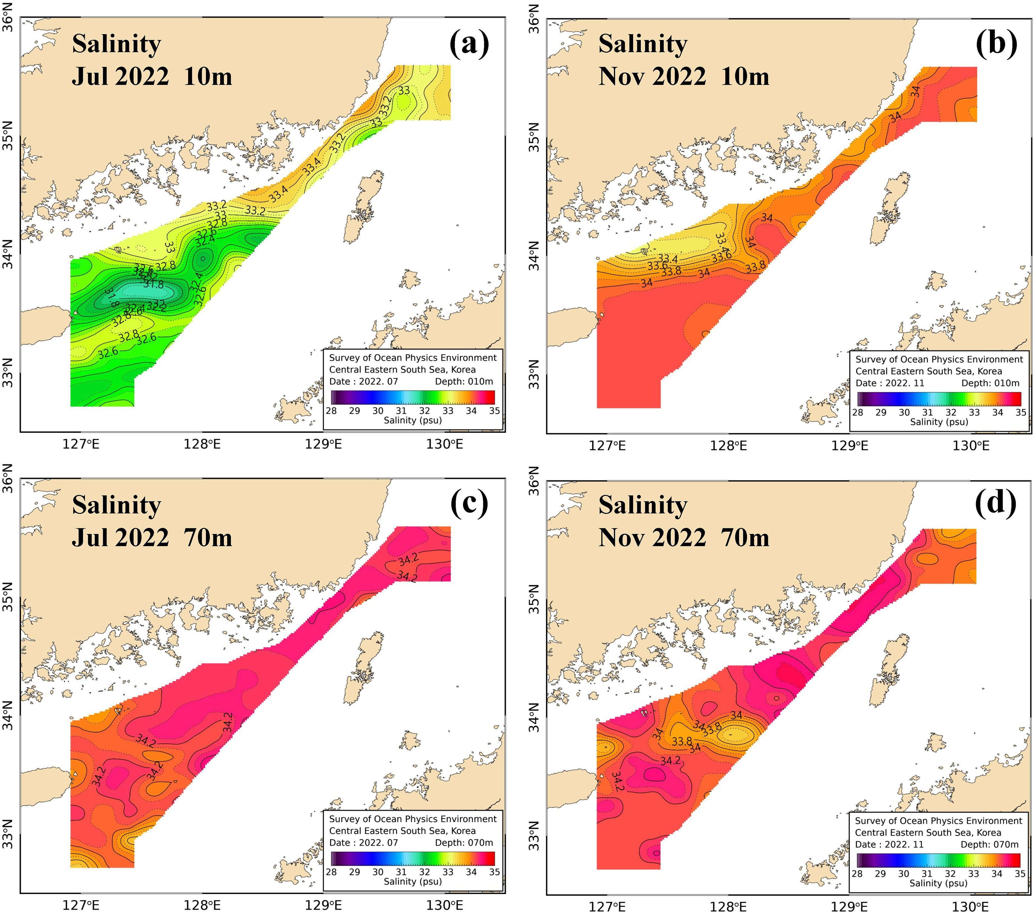
Figure 3. Horizontal distributions of salinity at 10 m and 70 m in July and November 2022: (a) July at 10 m, (b) November at 10 m, (c) July at 70 m, and (d) November at 70 m.
3.1.2 T–S structure and water mass properties
The T–S diagram of the study area (Supplementary Figure S2) showed two dominant water mass distribution characteristics. First, the warm saline water, with salinity of 34.0–34.7 and temperature of 12–27 °C, corresponded to the seasonal temperature and salinity characteristics of the Tsushima Warm Current (a branch of the Kuroshio) entering the East Sea (Sea of Japan) through the Korea Strait from the East China Sea (Teague et al., 2002; Takikawa et al., 2005; Isobe, 2008). Second, the low-salinity (≤ 32.3 psu) and high-temperature (20–28 °C) water, which was pronounced in July and September, corresponded to the eastward and northeastward extension of the Changjiang Diluted Water (CDW); this was consistent with satellite observations, in-situ measurements, and numerical studies showing the passage of CDW through Jeju Strait into the southern coastal waters (Lie et al., 2003; Chang and Isobe, 2003; Kim et al., 2009; Son and Choi, 2022). Additionally, in the eastern part of the southern coastal waters in September, the expansion of low-salinity surface water was pronounced due to freshwater inflow from coastal rivers (Baek et al., 2019; Yoon et al., 2022).
3.2 Vertical stability and stratification
3.2.1 Distributions of stability
Presented in Figure 4, the stability distribution exhibited a typical vertical gradient, with stronger stability in the upper layer and weaker stability in the deeper layers. The mean N² over the entire study area was 1.3 × 10⁻⁴ s−² at 10 m and 0.7 × 10⁻⁴ s−² at 80 m, showing a gradual decrease with depth (Supplementary Table S1). The spatial and seasonal patterns were characterized by enhanced stability in the upper layer during July–September and weakened stability in May and November. In particular, a high-stability band at 10 m formed in the northeastern waters of Jeju Island and extended to the eastern portion of the southern coastal waters in July (Figure 4A; Supplementary Figure S3). At 30 m in July, stability in the northeastern waters of Jeju Island was relatively low, while it remained high in the southeastern waters (Supplementary Figure S3). In September, compared to the surface layer, stability gradually increased along the coastal side below 30 m, and a gradual increase was observed across the entire study area at 50 m (Supplementary Figure S3). Vertical cross-section distributions also revealed seasonal variations, with an extensive high-stability band developing in the upper layer during July, which became fragmented and contracted by September, and mostly disappeared by November (Supplementary Figure S4). This high-stability band was shallower and stronger on the coastal side, while it was deeper and weaker on the offshore side of the study area (Supplementary Figure S4).
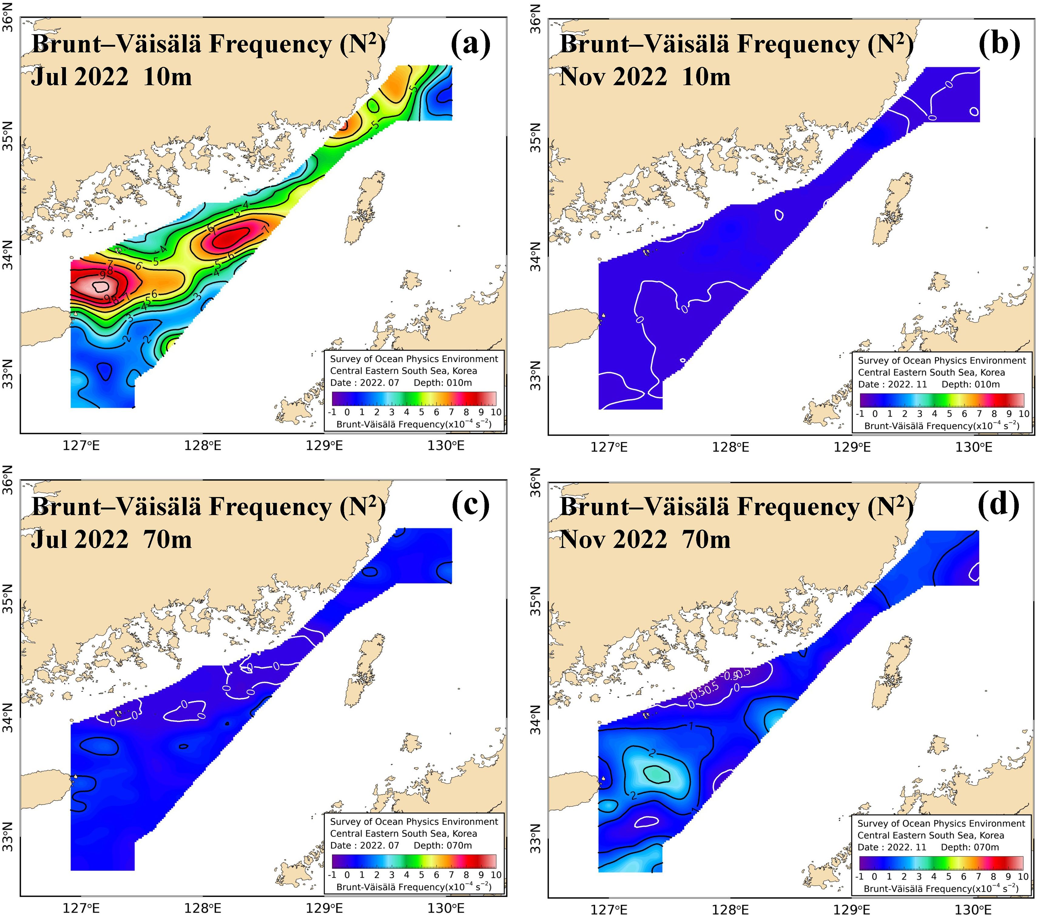
Figure 4. Horizontal distributions of Brunt–Väisälä frequency (N², × 10−4 s−²) at 10 m and 70 m in July and November 2022: (A) July at 10 m, (B) November at 10 m, (C) July at 70 m, and (d) November at 70 m.
3.2.2 Structure of vertical stratification
Figure 5 presents the seasonal horizontal distributions of TD, HD, and ΔTHD. TD had a mean depth of 60 m in May, 31 m in July, 64 m in September, and 69 m in November, becoming shallower in July and gradually deepening in September and November (Figures 5A, B; Supplementary Table S2). These seasonal variations were more pronounced in the northeastern waters of Jeju Island and the eastern part of the southern coastal waters, while TD gradually increased in deeper regions such as the southeastern waters of Jeju Island, the Korea Strait, and the southern waters of the East Sea (Sea of Japan) (Figures 5A, B). The distribution of HD showed similar seasonal patterns to TD, with mean values of 53 m in May, 23 m in July, 58 m in September, and 69 m in November (Figure 5C, D; Supplementary Table S2). However, HD exhibited greater seasonal variability and responsiveness, more pronounced spatial gradients between coastal and offshore waters, and greater regional variability than TD (Figures 5C, D).
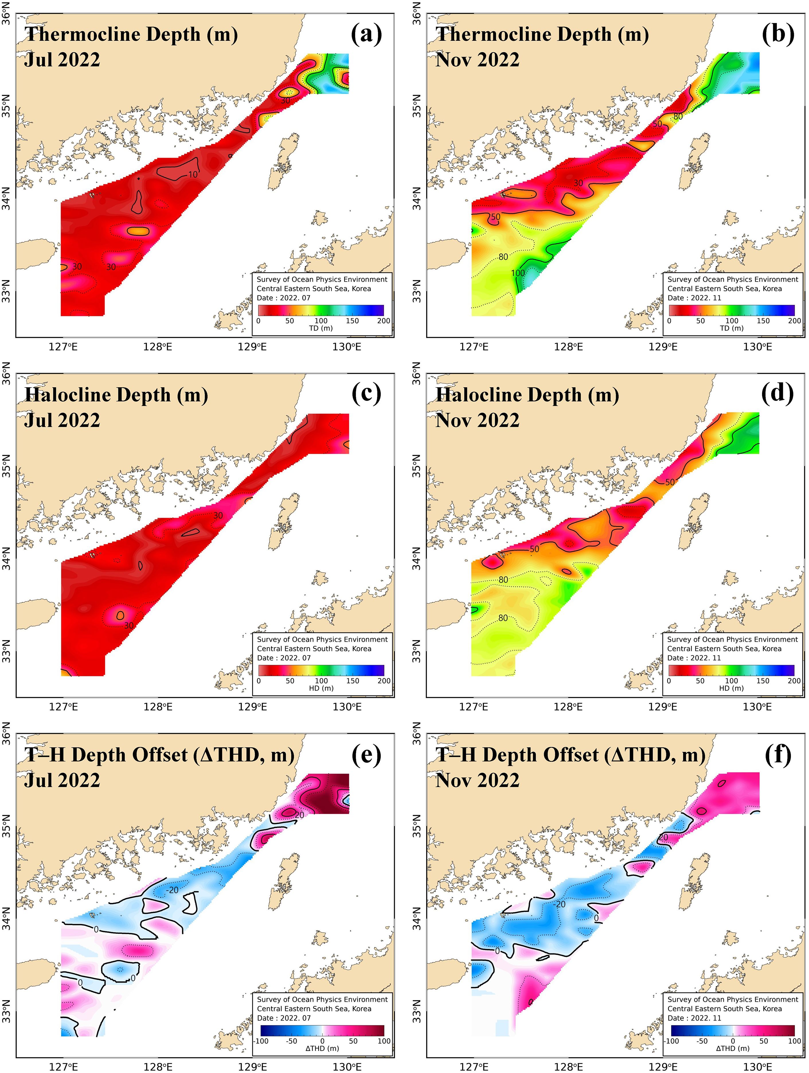
Figure 5. Horizontal distributions of thermocline depth (TD), halocline depth (HD), and their offset (ΔTHD = TD − HD) in July and November 2022. Positive values indicate a deeper thermocline than halocline, and negative values indicate a shallower thermocline: (A) TD in July, (B) TD in November, (C) HD in July, (D) HD in November, (E) ΔTHD in July, and (F) ΔTHD in November.
The distributions were dominated by small values within the range of −10 to +10 m in most regions, with more frequent occurrence of weakly positive values (Figures 5E, F). In May, the variability was most pronounced, with strong negative values below −50 m and strong positive values above +50 m juxtaposed along the western boundary of the study area (eastern coast of Jeju Island). In July, regions with more negative than −10 m were distributed in the northeastern waters of Jeju Island and the eastern portion of the southern coastal waters (Figure 5E). In September, an east–west band of approximately ±20 m developed in the eastern waters of Jeju Island. In November, a broad band of negative values extended from the northeastern waters of Jeju Island to the eastern part of the southern coastal waters (Figure 5F). At the eastern boundary of the study area (adjacent to the Korea Strait), strong positive values exceeding +30 m were observed throughout the year.
3.3 Spatial structure of IFI fronts and spatial agreement with conventional criteria
3.3.1 Composition and weighting of the IFI
In the IFI calculation presented in Section 2.2.3, represents a signed relative weight in which a positive value indicates that an increase in the corresponding component strengthens the IFI, whereas a negative value indicates weakening. The depth-averaged loadings were , , and , indicating that was dominant. In the surface layer, positive values were dominant across the entire study area, but some negative values were present in the eastern waters of Jeju Island. In the deep layer, positive values were also dominant, but broad negative regions were present, particularly in the eastern part of the southern coastal waters (Supplementary Figure S5).
Using α–β layer weights, we recomputed with the same per-depth top-15% threshold. Bilateral spatial agreement with the PCA-weighted masks was high (depth-averaged 76.3% for Cov( ← ), 86.8% for Cov( ← )); agreement is strongest at 10–40 m and slightly weaker at 50–70 m (Supplementary Table S3).
Threshold sensitivity confirms robustness: using 10%, 15%, and 20% per-depth cutoffs leaves spatial patterns unchanged. The depth-averaged spatial agreement of by the salinity-front mask increases from ~83% (10%) to ~90% (15%) and ~91% (20%), while overlaps with the temperature-gradient mask and with the intersection of the temperature- and salinity-gradient front masks remain ~71–76%. The spatial agreement of the intersection of the temperature- and salinity-gradient front masks with IFI is essentially stable at ~70% across thresholds.
3.3.2 Spatial and seasonal structures of IFI fronts
IFI fronts were defined by masking based on the top-15% threshold of the IFI score; the thick, black contour lines in Figure 6 indicate the frontal boundaries that exceeded this threshold. Overall, the fronts exhibited a continuous band-shaped pattern along the 80–100-m isobath, extending from the eastern waters of Jeju Island to the eastern part of the southern coastal waters (Figure 6). In May, a relatively uniform east–west-oriented front formed in the northeastern waters of Jeju Island, while in July, fronts expanded extensively within the upper 30-m layer. In September, fronts were broadly distributed along the southern coast below 30 m, rather than near the surface layer, while in the southeastern waters of Jeju Island, a front was present at 50 m. In November, the areas of fronts within the upper 50 m generally contracted, and fronts instead formed below 70 m, particularly in the southeastern waters of Jeju Island (Figure 7). In summary, fronts in the study area could be classified into continuous band-shaped fronts along the 80–100-m isobaths and broad frontal zones oriented northeast–southwest in the southeastern waters of Jeju Island. From May to July, fronts expanded and intensified in the upper layer, whereas from September to November, the upper-layer fronts gradually contracted and the formation depth of fronts deepened, indicating marked seasonal variability (Figure 7).
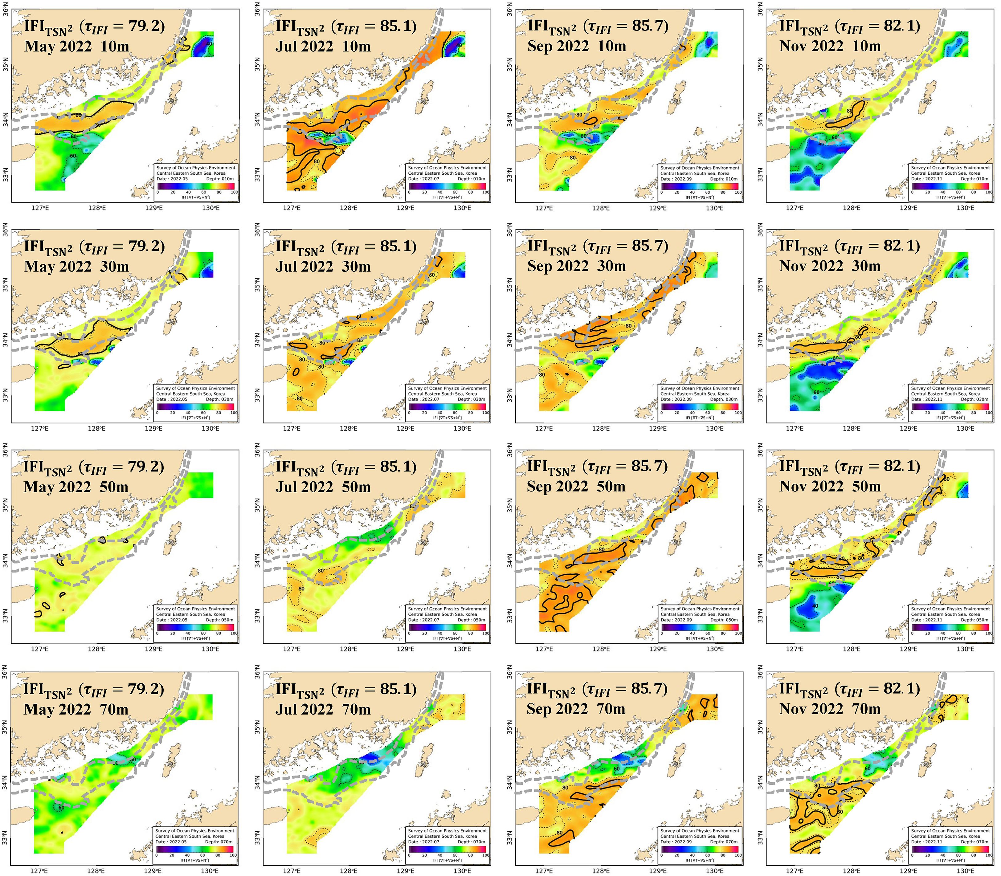
Figure 6. Horizontal distributions of at depths of 10, 30, 50, and 70 m. The first, second, third, and fourth columns correspond to May, July, September, and November 2022, respectively. Thick black contours denote the IFI fronts, defined by the 85th percentile threshold (top-15% threshold; τIFI = 79.2 in May, 85.1 in July, 85.7 in September, and 82.1 in November). Light gray dashed lines indicate the 70 and 100 m isobaths.
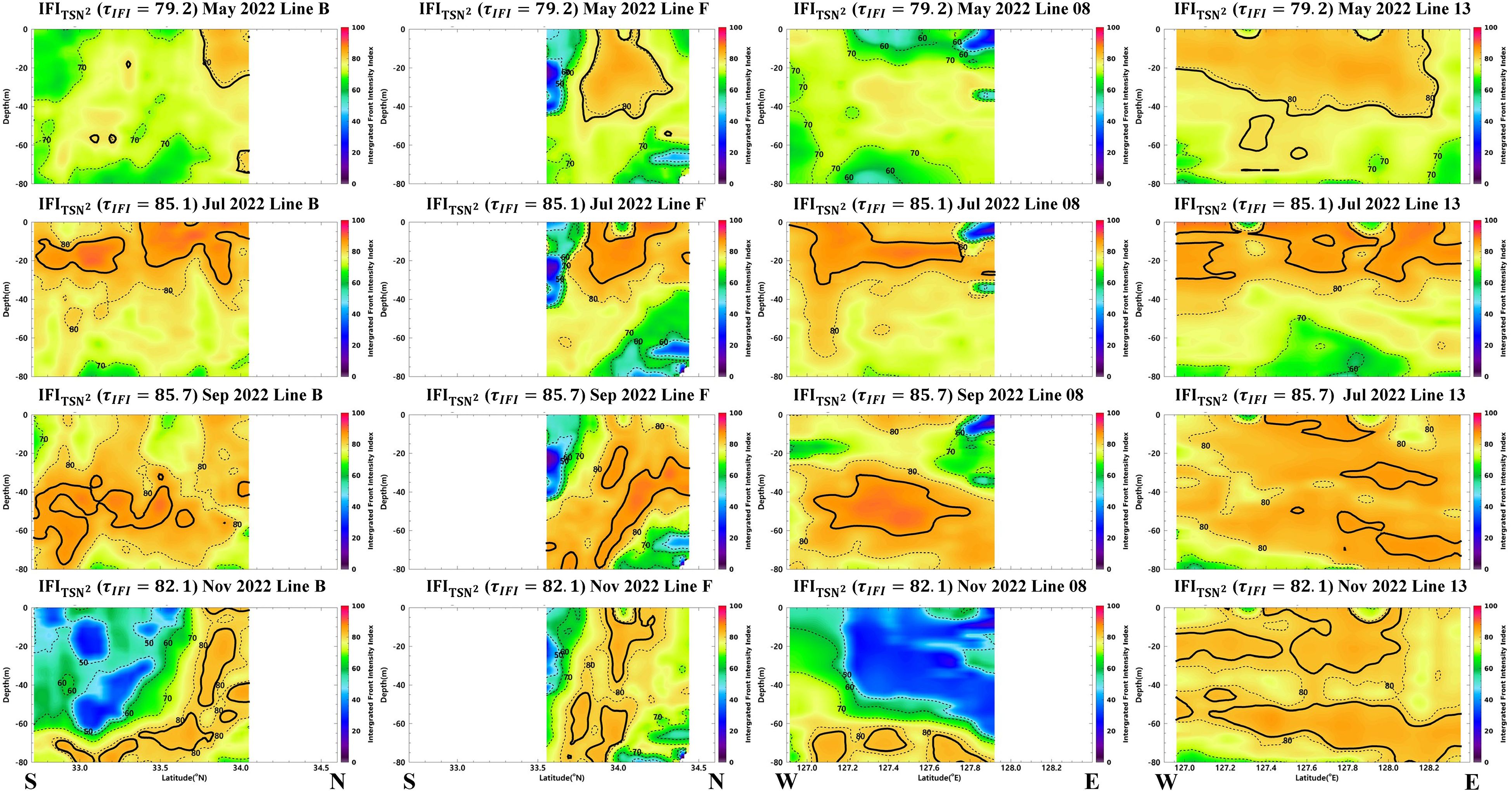
Figure 7. Vertical sections of along observational lines. The first, second, third, and fourth columns correspond to Lines B, F, 08, and 13, respectively, and rows represent May, July, September, and November 2022. Thick black contours denote the IFI fronts, defined by the 85th percentile threshold (top-15% threshold; τIFI = 79.2 in May, 85.1 in July, 85.7 in September, and 82.1 in November).
3.3.3 Spatial agreement with conventional fronts
Conventional fronts defined using a temperature gradient threshold of and a salinity gradient threshold of were compared with the top-15% IFI fronts (Table 2). Spatial agreement between temperature- and salinity-gradient fronts was approximately 76–78% at 10–30 m and about 48% at 80 m, indicating that the two front types did not consistently trace the same structures throughout the water column. Spatial agreement between the IFI and temperature-gradient fronts was high at 10–30 m (approximately 87–93%), decreased to about 63–55% at 40–50 m, and reached a minimum of about 48% at 70 m, and partially recovered at 80 m (≈71%). Spatial agreement between the IFI and salinity-gradient fronts was highest across all depths, approaching nearly 100% at 10–30 m and 60 m, while remaining around 74–75% at 40–50 m and 70–80 m. Triple spatial agreement among the three indices was high at 10–30 m (approximately 87–93%), decreased to 63–55% at 40–50 m, increased again to about 78% at 60 m, and reached a minimum of about 48% at 70 m, with a depth-averaged value of approximately 75%. In summary, while the two conventional criteria exhibited only partial agreement across the entire water column, salinity-gradient fronts most consistently captured the composite fronts defined by the IFI. Through its strong overlap with conventional information, the IFI demonstrated its potential to serve as a substitute (or an equivalent-level complement) in the form of a single, integrated index.
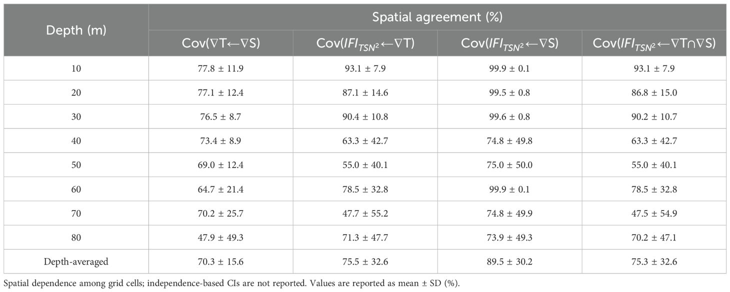
Table 2. Depth-dependent spatial agreement (%) between different frontal definitions: temperature-gradient versus salinity-gradient fronts, versus temperature-gradient fronts, versus salinity-gradient fronts, and the triple spatial agreement among , temperature-gradient, and salinity-gradient fronts. Values shown as mean ± SD.
3.4 Effect of stratification on fronts
Throughout the following comparisons, IFI should be read as a composite diagnostic that preserves the conventional (, ) definition of a front while explicitly embedding its stratification context (N²). Accordingly, isolates the net contribution of stability to the depth‐dependent expression of fronts. In a baroclinic ocean, the horizontal density gradient and stratification determine the vertical shear via the thermal wind relation. Increases in baroclinicity sharpen and confine frontal structures vertically (amplification), whereas reductions have the opposite effect (Vallis, 2017; Cushman-Roisin and Beckers, 2011).
To evaluate the effect of including the stability term, the stability-inclusive integrated index and the stability-excluding index were directly compared using the same threshold (top 15%) (Section 2.2.3). The difference between the two indices was defined as , with positive values indicating frontal intensification due to the inclusion of stability and negative values representing weakening. We interpret as the stratification’s net imprint on frontal expression. Positive values mean that the stratification sharpens and confines an existing T/S front. Negative values, on the other hand, arise from either thermohaline compensation, in which and oppose each other, reducing the horizontal density contrast (Rudnick and Ferrari, 1999; Rudnick and Martin, 2002), or from mixing/forcing (e.g., wind or tides) that lowers N2 and relaxes vertical confinement (Garrett and Kunze, 2007). In practice, the orientation of and , i.e. whether they are aligned or oppose each other, helps to distinguish these cases.
3.4.1 Contrasts and agreement of stratification effects
values compared at the same threshold were dominated by negative values; however, the magnitude and variability systematically differed with depth and season (Figure 8; Supplementary Figure S6). At 10-m depth, the mean value was −5.7, representing the strongest negative deviation. Below that, the deviation gradually decreased with increasing depth, reaching a minimum of −1.3 at 60 m, before increasing again to −4.6 at 80 m. This vertical trend appeared as a band-shaped structure along the 70–100-m isobaths extending from the northeastern waters of Jeju Island to the eastern part of the southern coastal waters, which was characterized by marked patterns of surface weakening, mid-layer mitigation, and deep-water re-weakening. Seasonally, the mean ΔIFI values in July and September were small at −1.4 and −1.8, respectively, while the strongest negative deviation occurred in November at −6.2. In July, small positive regions were scattered at 10–30 m, whereas in November, broad negative regions expanded linearly at 10–40 m, forming a distinctive feature. Agreement between the two indices’ front masks averaged 72% overall, with its highest values of around 80% in the upper layer (10–30 m), decreasing at 40 m, and lowest at 80 m. Seasonally, agreement was relatively low in May–July (approximately 67–68%), moderate in September (about 70%), and highest in November (about 83%).
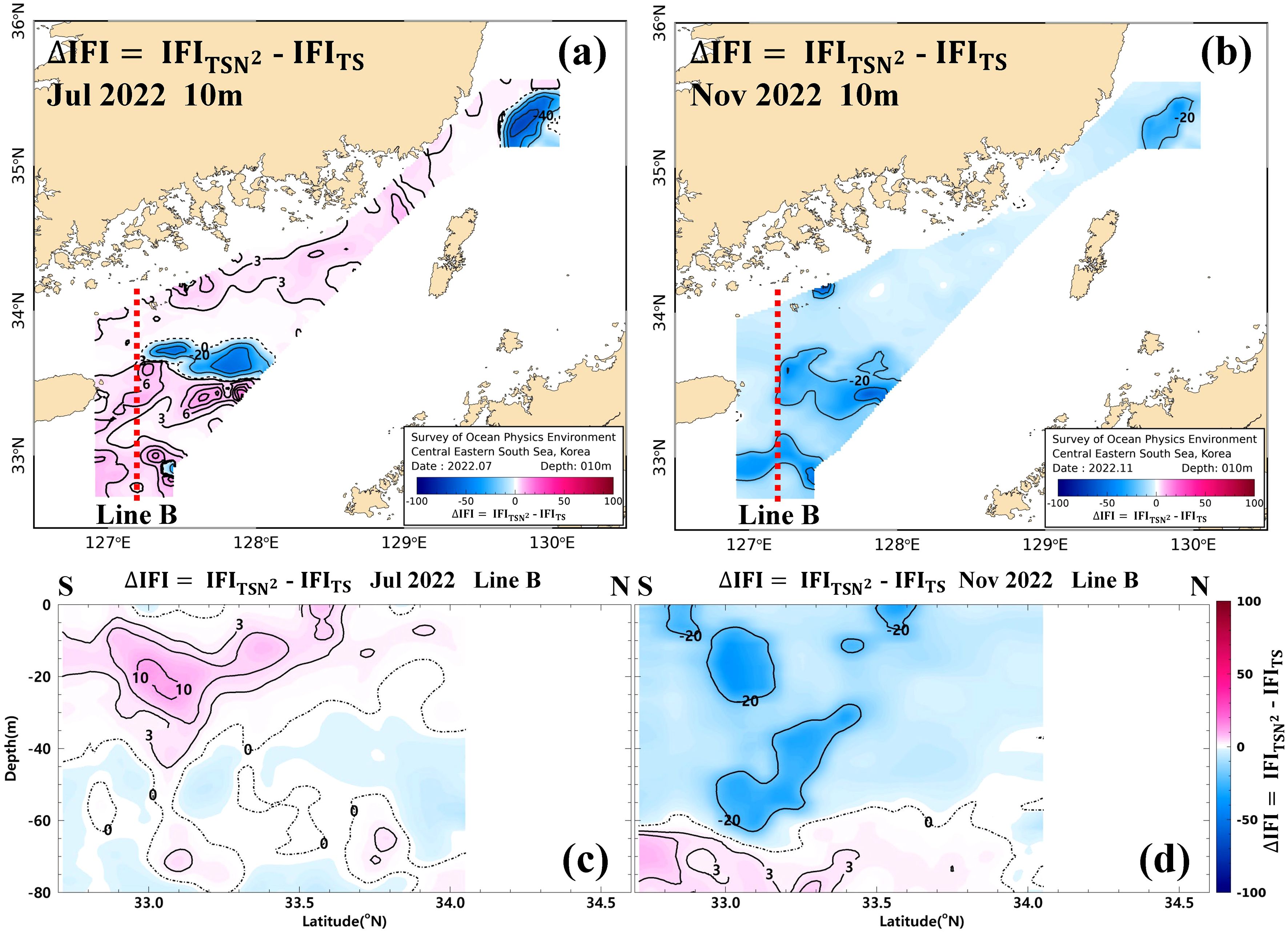
Figure 8. Distributions of ΔIFI ( – ) in July and November 2022: (a) July at 10 m, (b) November at 10 m, (c) vertical section along Line B in July, and (d) vertical section along Line B in November. Positive values indicate enhanced frontal intensity, whereas negative values indicate weakened intensity.
3.4.2 Linkage with thermocline–halocline alignment
Thermocline–halocline alignment is a key background variable that must be considered to fully characterize frontal variations, as it is directly related to how consistently temperature and salinity gradients lead to density stratification. Thermocline–halocline alignment is defined as ∣ΔTHD∣ = ∣TD − HD∣. The agreement and distribution of the two IFI front masks were summarized across these three intervals: ∣ΔTHD∣ < 10 m (hereafter, A1), 10 < ∣ΔTHD∣ < 30 m (hereafter, A2), and ∣ΔTHD∣ > 30 m (hereafter, A3).
Throughout the entire study area and period, the areal fractions of the three intervals were approximately 45.7% for A1, 32.6% for A2, and 21.7% for A3 (Supplementary Table S5). Seasonally, the fraction of A1 expanded to about 63.9% in July, while in November, A1 decreased to about 45.1% and A2 increased to about 37.1%. The A1 fraction was relatively large in the upper layer, while the fractions of A2 and A3 tended to increase with depth. Mean was slightly negative across all three intervals, and agreement between the two front masks was 62.2% for A1, 58.6% for A2, and 56.0% for A3, showing a gradual decrease with increasing ∣ΔTHD∣ (Table 3). The seasonal mean exhibited its largest differences at 10 m in all three intervals (−4.9, −5.6, and −4.0, respectively). It decreased with increasing depth, reached a minimum at 60–70 m, and then slightly increased at 80 m, showing a consistent trend. Agreement among the three intervals ranged from a minimum of about 68% to a maximum of about 88% at 10–30 m, with this layer showing the largest differences, while at 40–50 m and 70–80 m, the agreement was generally lower at about 28–44%. The depth-averaged showed the smallest differences in July (−1.7, −1.6, and −0.3, respectively) and the largest differences in November (−6.1, −5.9, and −5.3, respectively), while agreement also exhibited seasonal variability, being lowest in July and highest in November (Table 3).
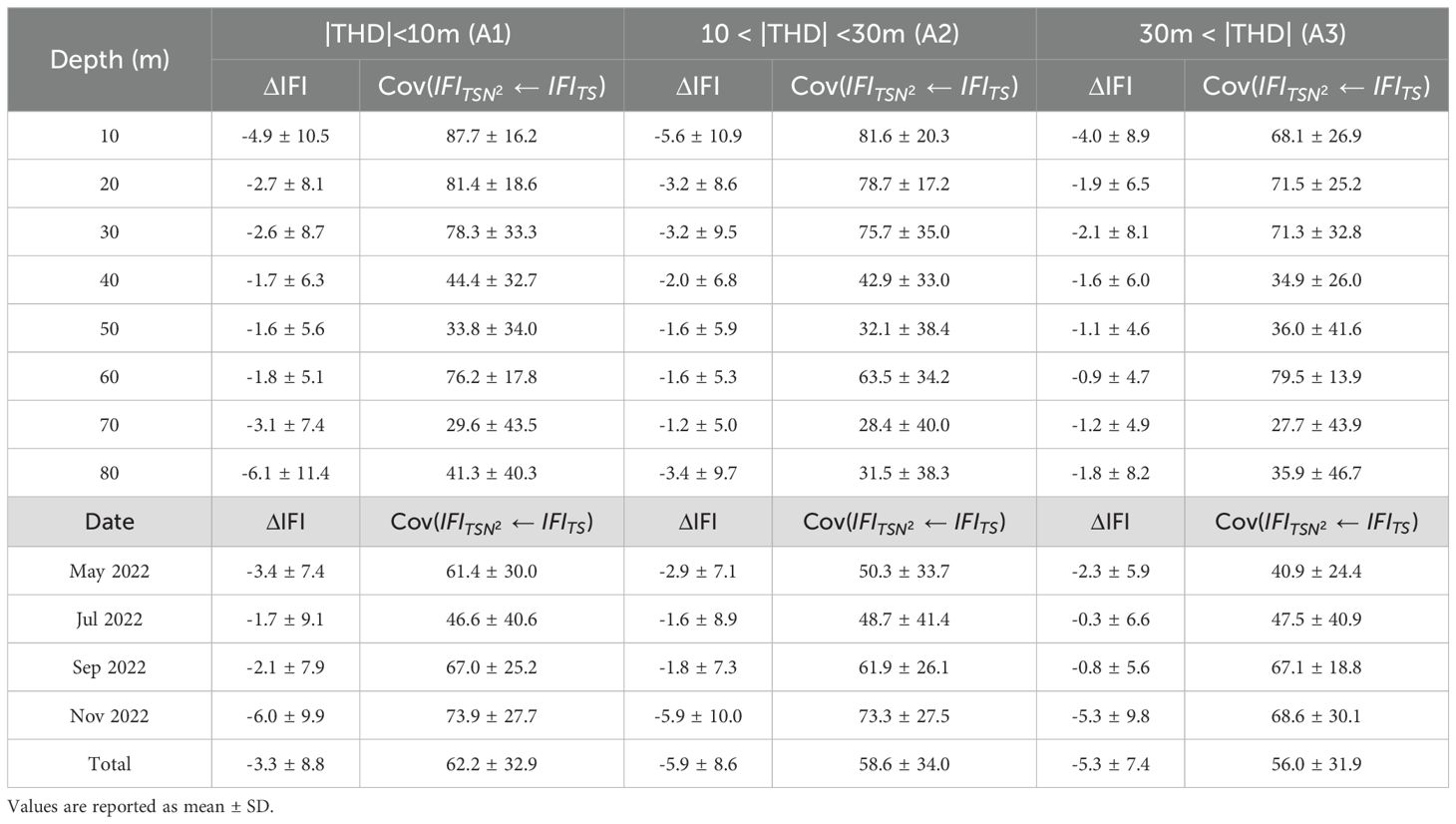
Table 3. Mean and standard deviation of ΔIFI, along with spatial agreement (%) between and , classified by the three ranges of ∣THD∣ (A1: ∣THD∣ < 10 m, A2: 10 < ∣THD∣ < 30 m, A3: ∣THD∣ > 30 m), for each depth layer and observation period.
4 Discussion
4.1 Regional hydrographic setting and observed patterns
The study area is a coastal–offshore transition zone linked to the shallow waters of the northern East China Sea, where the inflow of the Tsushima Warm Current (a branch of the Kuroshio), strong tidal forcing, complex topography, and summer freshwater influence overlap. Observations showed that horizontal water properties exhibit distinct coastal–offshore contrast, with surface warming and low salinity intensifying in summer but weakening and extending downward in autumn. Vertical stability (N2) increased in the upper layer from July to September, repeatedly forming high-stability bands along the coastal–offshore boundary zones. In November, these bands weakened and deepened. The thermocline gradually shoaled from spring to autumn, whereas the halocline deepened. The relative depth difference between the two clines (ΔTHD) tended to increase toward offshore regions.
Against this background field, the frontal structure could be summarized into two spatial modes: continuous band-shaped frontal zones formed along the coastal–offshore boundary (approximately 70–100-m isobaths) and a broad frontal zone in the southeastern offshore waters of Jeju Island. As the season progressed, the principal formation depths of the fronts gradually deepened. While spatial agreement with conventional fronts was generally high, it exhibited a depth-dependence, decreasing with increasing depth. Band-shaped fronts forming in coastal–offshore boundary zones have been repeatedly reported in continental shelf–open ocean transition zones of the northwestern Pacific (Park and Chu, 2006; Castelao and Wang, 2014). These observations are consistent with the band structures identified along the coastal–offshore boundary zones in the present study. In addition, this study extends previous findings by considering vertical structures at the same locations, thereby revealing depth-dependent patterns.
4.2 Stratification regime and thermocline–halocline alignment
The spatiotemporal variability of fronts is modulated by the phase of seasonal stratification and the alignment of the thermocline and halocline. In summer (July–September), enhanced surface buoyancy generally led to co-location of the thermocline and halocline, resulting in small ∣ΔTHD∣ values. At the same depth, temperature and salinity gradients run in the same direction, forming a single and consistent pycnocline. During this period, was comparable to , or showed slight enhancement in localized coastal and boundary zones. In contrast, in late autumn (November), surface cooling, wind-driven mixing, and the redistribution of freshwater enhanced thermohaline compensation, leading to an increase in ∣ΔTHD∣, while yielded relatively low frontal intensities (with ΔIFI shifting in the negative direction) and the effective density gradients tended to weaken even under the same horizontal gradients. This mechanism, in which alignment leads to amplification, whereas compensation results in weakening, has been proposed as a general explanatory framework in studies of the continental shelf near the East China Sea and the Korea Strait (Lie et al., 2003; Park and Chu, 2006). The present study refines this framework into observation-oriented diagnostics using ∣ΔTHD∣ and ΔIFI.
Vertically, the coupling effect on stability showed a consistent pattern of being strongest in the upper layer (10–30 m), weakest in the mid-layer (60–70 m), and renewed in the deeper layer (around 80 m). This pattern arises because stratification in the upper layer supports baroclinic shear, leading to stronger expression of frontal signals. At the transition zone, the balance between shear and mixing reduced the differences between the two indices. Meanwhile, in deeper layers, the influence of shear-driven mixing increased, once again amplifying the differences. Such inter-layer adjustments were pronounced along the coastal–offshore boundary.
4.3 Bathymetric dynamical controls on frontal structure
The organization of fronts in coastal–offshore boundary zones (approximately the 70–100-m isobaths) suggests that this region serves as a dynamical framework in which frontogenesis primarily occurs. In the Bohai–Yellow–East China Seas, topographic gradients, water mass boundaries, coastal currents, vertical shear, and mixing collectively determine the preferred regions of frontogenesis and the seasonal variability of fronts (Chen, 2009). In the upper boundary layer, isopycnal slopes and coastal current shear sustain and amplify horizontal contrasts, whereas turbulent mixing driven by internal tides, as well as shear and strain induced by topography, reorganize the vertical structure of the fronts. This interpretation is consistent with the spatial patterns of internal tide-induced mixing reported in the East China Sea, the continental shelf and slope region, and at the entrance to the Korea Strait (Niwa and Hibiya, 2004; Lozovatsky et al., 2008; Lien et al., 2013; Wang et al., 2022; Wijesekera et al., 2022, 2023).
Any linkage between the observed frontal modulation and mixing driven by internal tides is treated as a testable hypothesis rather than a conclusion. As a concrete next step, a targeted analysis of the spatial correlation between ΔIFI hotspots and strong topographic gradients along the 70–100-m isobaths within the coastal–offshore boundary zones could provide supporting evidence. Foundational reviews and regional studies highlight internal-tide generation by barotropic flow over strong topographic gradients of the continental shelf and slope and its role in enhanced mixing (Garrett and Kunze, 2007; Nash et al., 2012). The depth-dependent pattern of ∣ΔIFI∣ (maximized in the upper layer, minimized in the mid-layer, and increasing again in the deeper layer) suggests that gradients in shear and mixing regulate front–stratification coupling through inter-layer adjustment. Spatially, continuous frontal bands nearly parallel to the coastal–offshore boundary zones predominated. However, topographic features such as bends or constrictions of isobaths locally enhanced shear and mixing, leading to segmentation and directional shifts of the frontal bands.
The intensity and principal formation depths of the fronts are governed by offshore water inflow, the intermittent expansion of low-salinity surface waters in summer, and the relative strength of seasonal cooling and wind-driven mixing. Strong stratification in the upper layer promotes the expansion of salinity-gradient-dominated domains, which in turn maintains strong spatial agreement between conventional fronts and IFI fronts. This dominance of salinity gradients is in accordance with previous findings that salinity gradients are especially effective for identifying fronts in continental shelf regions (Chen et al., 2019) and is further corroborated by the high spatial agreement between IFI fronts and salinity-gradient-based fronts observed in this study. During the transition to the destratification period, surface stratification weakens and deepens, with thermohaline compensation occurring more frequently; as a result, fronts diffuse and weaken, and their principal formation depths shift deeper. Such seasonality of circulation and water masses, operating on the dynamical framework of the boundary zone, regulates the amplitude of fronts in a manner consistent with the seasonal and depth dependence of ΔIFI.
Taken together, several limitations qualify these findings. The analysis is confined to a single-year, bimonthly survey from May to November 2022, so the winter mixing period and longer-term variability are not covered, and the station spacing and cadence leave temporal and spatial gaps that may smooth or alias short-lived features. In addition, our OI mapping assumes an isotropic Gaussian with a fixed length scale, which can smooth small-scale anisotropy and raise in sparse or boundary regions; consequently, horizontal gradients near gaps and edges may be biased low whereas the large-scale patterns remain robust. Finally, the scope of sensitivity checks is limited to the percentile thresholds used (10–20%) and to the α–β layer weighting alternative; a broader season- and depth-specific analysis is deferred to future studies.
5 Conclusion
This study used CTD observations from May to November 2022 to quantify the spatiotemporal variability of coastal fronts in the central–eastern sector of the southern Korean coastal waters and to characterize their coupling with water-column stability. A multivariate Integrated Frontal Index (IFI) that integrates temperature, salinity, and stability with conventional horizontal-gradient criteria, enabling comparative evaluation of frontal intensity, position, and principal formation depth. Fronts were most coherently organized along coastal–offshore boundary zones that follow the 70–100 m isobaths. Their intensity and formation depths were systematically regulated by the seasonal stratification regime and by thermocline–halocline alignment (ΔTHD), producing sharp and shallow fronts when clines co-located in summer, and diffuse and deeper fronts when cooling and mixing offset the clines in late autumn. The framework captured depth-dependent transitions between salinity- and temperature-dominated regimes and provided an observation-based diagnostic (ΔIFI) for front–stratification coupling. For operations, monitoring vertical stability and the relative positions of the clines along the boundary zone, together with spatial agreement between IFI and conventional fronts, offers a practical basis for front tracking and observing-system design.
Data availability statement
The datasets presented in this article are not readily available because The data are part of a security-sensitive program and are not publicly available. Upon reasonable request, standard-depth raw CTD and gridded fields can be provided, subject to security review, via the corresponding author. Requests to access the datasets should be directed to Eung Kim, ZXVuZ0BraW9zdC5hYy5rcg==.
Author contributions
BK: Writing – original draft, Formal Analysis, Conceptualization, Methodology. SeK: Methodology, Conceptualization, Writing – review & editing, Investigation. SoK: Investigation, Writing – review & editing, Validation. SL: Investigation, Writing – review & editing. EK: Writing – review & editing, Project administration, Supervision.
Funding
The author(s) declare that financial support was received for the research and/or publication of this article. This research is part of the “Development of Maritime Domain Awareness Technology for Sea Power Enhancement (PEA0332)” project funded by the Korea Institute of Ocean Science & Technology.
Acknowledgments
We are grateful to the crew members of “R/V Onnuri” and “R/V Ieodo” of the Korea Institute of Ocean Science and Technology (KIOST).
Conflict of interest
The authors declare that the research was conducted in the absence of any commercial or financial relationships that could be construed as potential conflicts of interest.
Generative AI statement
The author(s) declare that no Generative AI was used in the creation of this manuscript.
Any alternative text (alt text) provided alongside figures in this article has been generated by Frontiers with the support of artificial intelligence and reasonable efforts have been made to ensure accuracy, including review by the authors wherever possible. If you identify any issues, please contact us.
Publisher’s note
All claims expressed in this article are solely those of the authors and do not necessarily represent those of their affiliated organizations, or those of the publisher, the editors and the reviewers. Any product that may be evaluated in this article, or claim that may be made by its manufacturer, is not guaranteed or endorsed by the publisher.
Supplementary material
The Supplementary Material for this article can be found online at: https://www.frontiersin.org/articles/10.3389/fmars.2025.1723724/full#supplementary-material
Supplementary Figure 1 | Horizontal distributions of (a) temperature and (b) salinity at depths of 10, 30, 50, and 70 m. The first column corresponds to May 2022, the second to July 2022, the third to September 2022, and the fourth to November 2022.
Supplementary Figure 2 | Temperature–salinity (T–S) diagram constructed from all CTD observations during the study period. Green, red, yellow, and blue dots represent May, July, September, and November 2022, respectively.
Supplementary Figure 3 | Horizontal distributions of Brunt–Väisälä frequency (N², × 10⁻4 s⁻²) at depths of 10, 30, 50, and 70 m. The first, second, third, and fourth columns correspond to May, July, September, and November 2022, respectively.
Supplementary Figure 4 | Vertical sections of Brunt–Väisälä frequency (N², × 10⁻4 s⁻²) along observational lines. The first, second, third, and fourth columns correspond to Lines B, F, 08, and 13, respectively, and rows represent May, July, September, and November 2022.
Supplementary Figure 5 | (A) Horizontal distributions of PC1 loadings derived from PCA for temperature gradient (ωt), salinity gradient (ωs), and Brunt–Väisälä frequency (ωN²). The first row shows ωt at 10 and 70 m, the second row ωs, and the third row ωN². (B) Vertical profiles of mean PC1 loadings for ωt (black), ωs (blue), and ωN² (red).
Supplementary Figure 6 | Horizontal distributions of ΔIFI ( – ) at depths of 10, 30, 50, and 70 m. The first, second, third, and fourth columns correspond to May, July, September, and November 2022, respectively.
Supplementary Table 1 | Basic statistical results for temperature (°C), salinity (psu), and Brunt–Väisälä frequency (N², × 10⁻4 s⁻²) by depth.
Supplementary Table 2 | Basic statistical results of thermocline depth (m), halocline depth (m), and T–H depth offset (ΔTHD, m) by observation period.
Supplementary Table 3 | Depth-dependent bilateral spatial agreement (%) between the α–β layer-weighted and the PCA-weighted , using the same top-15% threshold at each depth. Values are reported as mean ± SD (%).
Supplementary Table 4 | Depth-dependent spatial agreement (%) between different frontal definitions: versus temperature-gradient fronts; versus salinity-gradient fronts, and the triple spatial agreement among , temperature-gradient, and salinity-gradient fronts; and versus . Values are reported as mean ± SD (%).
Supplementary Table 5 | Contribution (%) of ∣THD∣ classified into three ranges (A1: ∣THD∣ < 10 m, A2: 10 < ∣THD∣ < 30 m, and A3: ∣THD∣ > 30 m) by observation period and over the entire study period.
References
Baek S. H., Kim D., Kim Y. O., Son M., Kim Y. J., Lee M., et al. (2019). Seasonal changes in abiotic environmental conditions in the Busan coastal region (South Korea) due to the Nakdong River in 2013 and effect of these changes on phytoplankton communities. Cont. Shelf Res. 175, 116–126. doi: 10.1016/j.csr.2019.01.014
Belkin I. M., Cornillon P. C., and Sherman K. (2010). Fronts in large marine ecosystems. Prog. Oceanogr. 81, 223–236. doi: 10.1016/j.pocean.2009.04.015
Belkin I. M. and Zang Y.-T. (2025). South China sea SST fronts 2015–2022. Remote Sens. 17, 817. doi: 10.3390/rs17050817
Bretherton F. P., Davis R. E., and Fandry C. B. (1976). A technique for objective analysis and design of oceanographic experiments applied to MODE-73. Deep-Sea Res. Oceanogr. Abstr. 23, 559–582. doi: 10.1016/0011-7471(76)90001-2
Castelao R. M. and Wang Y. (2014). Wind-driven variability in sea surface temperature front distribution in the California Current System. J. Geophys. Res. Oceans. 119, 1861–1875. doi: 10.1002/2013JC009531
Chang P.-H. and Isobe A. (2003). A numerical study on the Changjiang diluted water in the Yellow and East China Seas. J. Geophys. Res. Oceans. 108, 3299. doi: 10.1029/2002JC001749
Chen C.-T. A. (2009). Chemical and physical fronts in the Bohai, Yellow and East China seas. J. Mar. Syst. 78, 394–410. doi: 10.1016/j.jmarsys.2008.11.016
Chen H., Ji Q., Wu Q., Peng T., Wang Y., and Meng Z. (2024). Seasonal variability and underlying dynamical processes of sea surface temperature fronts in zhoushan and its adjacent seas. J. Mar. Sci. Eng. 12, 2335. doi: 10.3390/jmse12122335
Chen H.-H., Qi Y., Wang Y., and Chai F. (2019). Seasonal variability of SST fronts and winds on the southeastern continental shelf of Brazil. Ocean Dyn. 69, 1387–1399. doi: 10.1007/s10236-019-01310-1
Cushman-Roisin B. and Beckers J. M. (2011). Introduction to geophysical fluid dynamics: physical and numerical aspects Vol. 101 (Waltham, MA, USA: Academic press).
Freeman N. M. and Lovenduski N. S. (2016). Mapping the Antarctic Polar Front: weekly realizations from 2002 to 2014. Earth Syst. Sci. Data. 8, 191–198. doi: 10.5194/essd-8-191-2016
Garrett C. and Kunze E. (2007). Internal tide generation in the deep ocean. Annu. Rev. Fluid Mech. 39, 57–87. doi: 10.1146/annurev.fluid.39.050905.110227
Gong Y. (1982). A study of oceanic thermal fronts in the southwestern Japan Sea. Bull. Fish. Res. Dev. Agency. 28, 25–54.
Hickox R., Belkin I., Cornillon P., and Shan Z. (2000). Climatology and seasonal variability of ocean fronts in the East China, Yellow and Bohai Seas from satellite SST data. Geophys. Res. Lett. 27, 2945–2948. doi: 10.1029/1999GL011223
Isobe A. (2008). Recent advances in ocean-circulation research on the Yellow Sea and East China Sea shelves. J. Oceanogr. 64, 569–584. doi: 10.1007/s10872-008-0048-7
Jolliffe I. T. and Cadima J. (2016). Principal component analysis: A review and recent developments. Philos. Trans. R. Soc A. 374. doi: 10.1098/rsta.2015.0202
Karati K. K., Vineetha G., Raveendran T. V., Muraleedharan K. R., Habeebrehman H., Philson K. P., et al. (2018). River plume fronts and their implications for the biological production of the Bay of Bengal. Indian Ocean. Mar. Ecol. Prog. Ser. 597, 79–98. doi: 10.3354/meps12607
Kawai H. (1972). “Hydrography of the kuroshio extension,” in Kuroshio, Its Physical Aspects. Eds. Stommel H. and Yoshida K. (Tokyo, Japan: University of Tokyo Press), 235–352.
Kim H.-C., Yamaguchi H., Yoo S., Zhu J., Okamura K., Kiyomoto Y., et al. (2009). Distribution of Changjiang Diluted Water detected by satellite chlorophyll-a and its interannual variation during 1998–2007. J. Oceanogr. 65, 129–135. doi: 10.1007/s10872-009-0013-0
Kim S.-H., Shin J., Kim D.-W., and Jo Y.-H. (2023). Estimation of subsurface salinity and analysis of Changjiang diluted water volume in the East China Sea. Front. Mar. Sci. 10. doi: 10.3389/fmars.2023.1247462
Lie H.-J., Cho C.-H., Lee J.-H., and Lee S. (2003). Structure and eastward extension of the Changjiang River plume in the East China Sea. J. Geophys. Res. Oceans. 108, 3077. doi: 10.1029/2001JC001194
Lien R.-C., Sanford T. B., Jan S., Chang M.-H., and Ma B. (2013). Internal tides on the East China Sea continental slope. J. Mar. Res. 71, 151–186. Available online at: https://elischolar.library.yale.edu/journal_of_marine_research/369 (Accessed November 7, 2025).
Liu Y., Wang J., Han G., Lin X., Yang G., and Ji Q. (2022). Spatio-temporal analysis of east Greenland polar front. Front. Mar. Sci. 9. doi: 10.3389/fmars.2022.943457
Lozovatsky I. D., Liu Z., Wei H., and Fernando H. J. S. (2008). Tides and mixing in the northwestern East China Sea. Part II: Near-bottom turbulence. Cont. Shelf Res. 28, 338–350. doi: 10.1016/j.csr.2007.08.007
Lynn R. J. (1986). The subarctic and northern subtropical fronts in the eastern north pacific ocean in spring. J. Phys. Oceanogr. 16, 209–222. doi: 10.1175/1520-0485(1986)016<0209:TSANSF>2.0.CO;2
Na J.-Y., Lee S.-W., and Cho K.-D. (1991). A study on sea water and ocean current in the sea adjacent to Korea peninsula-The vertical structure of temperatures in the East Sea of Korea. J. Korean Fish. Soc 24, 215–228.
Nash J. D., Kelly S. M., Shroyer E. L., Moum J. N., and Duda T. F. (2012). The unpredictable nature of internal tides on continental shelves. J. Phys. Oceanogr. 42, 1981–2000. doi: 10.1175/JPO-D-12-028.1
Niwa Y. and Hibiya T. (2004). Three-dimensional numerical simulation of M2 internal tides in the East China Sea. J. Geophys. Res. Oceans. 109, C04027. doi: 10.1029/2003JC001923
Park J. H. and Choi K. H. (1995). A study on the fishing ground and the prediction of fishing conditions of mackerel, Scomber Japonicus Houttuyn. Bull. Nat. Fish. Res. Dev. Agency. 49, 25–35.
Park S. and Chu P. C. (2006). Thermal and haline fronts in the Yellow/East China Seas: Surface and subsurface seasonality comparison. J. Oceanogr. 62, 617–638. doi: 10.1007/s10872-006-0081-3
Park K.-A., Chung J. Y., and Kim K. (2004). Sea surface temperature fronts in the East (Japan) Sea and temporal variations. Geophys. Res. Lett. 31, L07304. doi: 10.1029/2004GL019424
Park K.-A., Ullman D. S., Kim K., Chung J. Y., and Kim K.-R. (2007). Spatial and temporal variability of satellite-observed Subpolar Front in the East/Japan Sea. Deep-Sea Res. Part I. 54, 453–470. doi: 10.1016/j.dsr.2006.12.010
Pelegrí J. L., Claret M., and Sangrà P. (2024). Vertical shear, diapycnal shear and the gradient Richardson number. Oceans. 5, 785–804. doi: 10.3390/oceans5040045
Rudnick D. L. and Ferrari R. (1999). Compensation of horizontal temperature and salinity gradients in the ocean mixed layer. Science 283, 526–529. doi: 10.1126/science.283.5401.526
Rudnick D. L. and Martin J. P. (2002). On the horizontal density ratio in the upper ocean. Dyn. Atmos. Oceans 36, 3–21. doi: 10.1016/S0377-0265(02)00022-2
Schick R. S., Goldstein J., and Lutcavage M. E. (2004). Bluefin tuna (Thunnus thynnus) distribution in relation to sea surface temperature fronts in the Gulf of Maine, (1994>–96). Fish Oceanogr. 13, 225–238. doi: 10.1111/j.1365-2419.2004.00290.x
Shin J., Kim D.-W., Kim S.-H., Lee G., Khim B.-K., and Jo Y.-H. (2024). Gap-filling techniques applied to the GOCI-derived daily sea surface salinity product for the Changjiang diluted water front in the East China Sea. Earth Syst. Sci. Data. 16, 3193–3211. doi: 10.5194/essd-16-3193-2024
Son Y. B. and Choi J.-K. (2022). Mapping the Changjiang Diluted Water in the East China Sea during summer over a 10-year period using GOCI satellite sensor data. Front. Mar. Sci. 9. doi: 10.3389/fmars.2022.1024306
Takikawa T., Yoon J.-H., and Cho K.-D. (2005). The Tsushima Warm Current through Tsushima Straits estimated from ferryboat ADCP data. J. Phys. Oceanogr. 35, 1154–1168. doi: 10.1175/JPO2742.1
Teague W. J., Jacobs G. A., Perkins H. T., Book J. W., Chang K.-I., and Suk M.-S. (2002). Low-frequency current observations in the Korea/Tsushima strait. J. Phys. Oceanogr. 32, 1621–1641. doi: 10.1175/1520-0485(2002)032<1621:LFCOIT>2.0.CO;2
Thomson R. E. and Emery W. J. (2014). Data Analysis Methods in Physical Oceanography. 3rd ed. (Amsterdam, Netherlands: Elsevier).
Ullman D. S. and Cornillon P. C. (1999). Satellite-derived sea surface temperature fronts on the continental shelf off the northeast US coast. J. Geophys Res-Oceans. 104, 23459–23478. doi: 10.1029/1999JC900133
Vallis G. K. (2017). Atmospheric and Oceanic Fluid Dynamics: Fundamentals and Large-Scale Circulation. 2nd edn (Cambridge, UK: Cambridge University Press). doi: 10.1017/9781107588417
Wang W., Robertson R., Wang Y., Zhao C., Hao Z., Yin B., et al. (2022). Distinct variability between semidiurnal and diurnal internal tides at the East China Sea shelf. Remote Sens. 14, 2570. doi: 10.3390/rs14112570
Wijesekera H. W., Jarosz E., Wang D. W., Luecke C. A., Teague W. J., Chang K.-I., et al. (2022). Tidally driven mixing “hot spot” at the entrance of the Japan/East Sea. Geophys. Res. Lett. 49, e2022GL100315. doi: 10.1029/2022GL100315
Wijesekera H. W., Luecke C. A., Wang D. W., Jarosz E., DeRada S., Teague W. J., et al. (2023). Mixing processes at the southwestern entrance to the Japan/East Sea. J. Phys. Oceanogr. 53, 2797–2821. doi: 10.1175/JPO-D-23-0061.1
Wolter K. and Timlin M. S. (2011). El Niño/Southern Oscillation behaviour since 1871 as diagnosed in an extended multivariate ENSO index (MEI.ext). Int. J. Climatol. 31, 1074–1087. doi: 10.1002/joc.2336
Yang J. Y., Kim S. H., and Rho H. K. (1998). A study on the temperature fronts observed in the South-West Sea of Korea and the northern area of the East China Sea. Korean J. Fish. Aquat. Sci. 31, 695–706.
Keywords: coastal–offshore transition zone, Integrated Frontal Index (IFI), oceanic fronts, Southern coastal waters of Korea, thermocline–halocline alignment, water column stability
Citation: Kim B, Kim S, Kwon S, Lee S and Kim E (2025) Seasonal frontal variability and stratification coupling from 2022 CTD observations in the southern coastal waters of Korea. Front. Mar. Sci. 12:1723724. doi: 10.3389/fmars.2025.1723724
Received: 13 October 2025; Accepted: 31 October 2025;
Published: 20 November 2025.
Edited by:
Francisco Machín, University of Las Palmas de Gran Canaria, SpainCopyright © 2025 Kim, Kim, Kwon, Lee and Kim. This is an open-access article distributed under the terms of the Creative Commons Attribution License (CC BY). The use, distribution or reproduction in other forums is permitted, provided the original author(s) and the copyright owner(s) are credited and that the original publication in this journal is cited, in accordance with accepted academic practice. No use, distribution or reproduction is permitted which does not comply with these terms.
*Correspondence: Eung Kim, ZXVuZ0BraW9zdC5hYy5rcg==