 W. A. Gray*
 R. S. Dwyer-Joyce
- Department of Mechanical Engineering, The Leonardo Centre for Tribology, University of Sheffield, Sheffield, United Kingdom
The lubricant inlet meniscus in a rolling element bearing acts as a reservoir that feeds the elastohydrodynamic contact, resulting in a sufficiently thick film to avoid wear. A shortening and/or thinning of the inlet meniscus towards the contact centre is an indicator of bearing starvation and impaired lubricant performance. This work introduces an ultrasonic method to measure meniscus dimensions. Using in situ ultrasonic sensors on a full-scale cylindrical roller bearing test rig, we show that ultrasonic waves can cause oil films to resonate, and that the resonant frequency is directly related to the film thickness. Using a benchtop rig we validate the relationship between resonant frequency and film thickness. This allows for the measurement of meniscus thickness and length in situ during bearing operation. Menisci were measured at both the inlet and outlet of rolling bearing line contacts while lubricated with different viscosity oils and grease. All lubricants used showed they could be monitored using this approach. The implication of this paper is that it is possible to measure a critically important lubrication mechanism during operation without major component modifications.
1 Introduction
Cylindrical roller bearings are common machinery components used for the support of exclusively radial loads acting on a rotating part. The support of this load, without causing wear, is achieved using a lubricating oil or grease which acts to separate surfaces within the bearing structure. Although there is lots of literature on the lubricant conditions within the contact, comparatively little is known about the meniscus which feeds lubricant to the contact.
Within bearings the opposing surface dimensions are non-conformal, and so the real area of contact is small causing high pressures. This leads to elastohydrodynamic lubrication (EHL) where surface separation is achieved from lubricant film thickening due to a viscosity-pressure relationship, and localised elastic deformation of asperities within the contact. For EHL line contacts Dowson and Higginson (1959) were the first to develop a numerical solution to predict minimum film thickness, and later Dowson and Toyoda (1978) extended the model to predict central film thickness. Despite more complicated models now existing, most are based on these original equations because of their relative ease of use and for their remarkable accuracy when compared with lab results Lubrecht et al. (2009). One issue with these models however is the “infinite meniscus” assumption. The meniscus is a body of lubricant that forms at the inlet to the contact and feeds oil into the contact so that the separating film can be maintained. By presuming it is infinitely long, it is assumed there is adequate lubricant for the film to develop and that any change in film thickness is due to other conditions such as load, bearing speed and viscosity.
In a real contact, the meniscus has a finite length, and this assumption becomes inappropriate, particularly for grease lubricated bearings which are known to operate under starved conditions Lugt (2009) Lugt (2013). Wedeven et al. (1971) was one of the first to question how this length may effect contact film thickness. They found that as the meniscus length shortens, and moves towards the Hertzian contact zone, the contact becomes starved, resulting in the contact film thickness reducing to a proportion of the fully flooded thickness. Wolveridge et al. (1970) addressed this starvation problem with a semi-analytical approach, and findings gave the same conclusion as Wedeven, as the meniscus length shortens, the load carrying capacity of rollers in a bearing reduces to a proportion of the fully flooded capabilities. More recently, Kumar et al. (2010) modelled contact starvation by moving the inlet meniscus position and found that shorter menisci lead to thinner films with higher coefficients of friction. Svoboda et al. (2013) used optical interferometry on a single ball contact to measure how central film thickness was affected by starvation and obtained results that agreed well with literature. Kostal et al. (2017) then used the same rig to vary the meniscus thickness and show the central film thickness dependency on this value.
It has so far been difficult to accurately measure meniscus length and thickness in situ within a rolling bearing of any kind, without component modifications. This is due to the menisci being very thin, occurring over small areas, and being hidden deep within the inner workings of a bearing. Cameron and Gohar (1966) developed a very accurate optical method for measuring thin oil films in the nanometer range, which has become popular for measuring meniscus dimensions Cann and Lubrecht (1999) Cen et al. (2014). However, this method requires a transparent window to the contact which limits the application to laboratory experiments. An alternative approach has been the capacitance method founded by Wilson (1979) and developed by Heemskerk et al. (1982) in which the electrical resistance is linked to a film thickness. This method has been used to study film thickness and starvation in bearings Cen and Lugt (2019) Cen and Lugt (2020). The downsides to this approach are that modifications are still needed as access is required either side of the contact, the measurement is an average of the film thickness of the inner and outer raceway, and free lubricant films cannot be measured. That is to say, one cannot measure a steel-oil-air layer that defines the meniscus away from the contact.
In the last 2 decades ultrasonic sensors have been gaining momentum as an alternative technology to measure bearing lubricant conditions Dwyer-Joyce et al. (2003) Dou et al. (2022). This is due largely to their low cost, simplicity, and ability to propagate waves through solid and liquid media, meaning direct contact access is not required. In this paper we have instrumented a bearing test rig with ultrasonic sensors and measured reflections from the steel-oil-air interface where the meniscus occurs. The wave interaction causes a measurable resonance that relates to the thickness of the oil, and by tracking these resonances it is possible to measure the meniscus thickness.
1.1 Background
Figure 1A shows a schematic of a solid-oil-air interface, that exists in the meniscus region of a contact, forming two boundaries at x = 0, h. Here, h is equivalent to the thickness of the oil film. It is assumed here that the boundaries are perfectly bonded and any wave travel is perfectly perpendicular to the boundaries. The acoustic impedance z of a material is the product of its density ρ and speed of sound c. When an ultrasonic wave strikes the boundary between two acoustically different materials, a portion transmits into the second material, and the remainder reflects. The reflection coefficient R quantifies the reflected proportion and is calculated in Eq. 1:
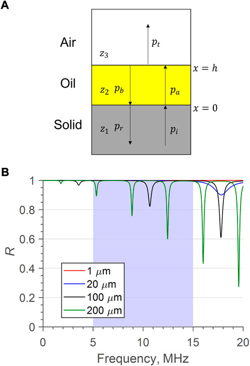
FIGURE 1. (A) schematic 3-body system showing the formation of transmitted and reflected waves. (B) Predicted Reflection coefficient using Eq. 6, resonances appear as dips in R. The blue region shows a typical usable bandwidth, centred around 10 MHz.
From this equation it is clear that greater acoustic mismatches lead to a greater proportion of the wave being reflected. In Figure 1A, pi represents the initial, incident wave pressure which has all of the wave energy. This then splits at the boundary between steel and oil where x = 0 and a transmitted wave pa and reflected wave pr form. The transmitted wave continues to the boundary at x = h and splits again at the oil boundary with air, into the transmitted pt and reflected pb. Where c2 is the speed of sound through the second material, the oil layer, and λ is the ultrasonic wavelength, if h is sufficiently large, to the point were 2h/c2 > λ, the reflections pr and pb will be observably distinct from one another. The time between reflections Δt can then be measured, and equates to:
Equation 2 can be rearranged to make h the subject, and so the thickness of the second body can be calculated. This is known as the Time-Of-flight method (TOF).
However, if h < λ the reflected signals pr and pb superimpose and are not distinct. The case of the complex reflection coefficient, from a layered material, in terms of pressure was given by Brekhovskikh (1960):
Where R12 and R23 are the reflection coefficients at the media boundaries at x = 0, h. α2 is a coefficient referring to the second medium, defined as:
Where β is the attenuation coefficient, k2 is the wave number calculated as:
where f is frequency.
Although Eq. 3 is complex, incorporating amplitude and phase, Haines et al. (1978) gives an equation for the real, amplitude portion:
Kinsler et al. (2000) explains when a wave travelling through an acoustically soft material reaches the boundary with an acoustically harder material z1 < z2 the reflected portion of the wave is perfectly in phase with the incident wave. When z1 > z2 the reflected wave is 180° out of phase with the incident wave. Transmitted and incident waves across a boundary are always in phase regardless of acoustic impedances at a boundary. These rules still hold true at x = 0, h in a 3-body system. However, the phase between the transmitted wave pa from the first boundary and the reflected wave pb from the second boundary changes based on the distance between boundaries i.e. the thickness of the middle layer. Haines et al. (1978) showed that when z2 > z3 the middle layer resonates if the phase between pa and pb is ± (2n + 1) π/2 where n is any integer value (n = 0, 1, 2, 3, …). At these particular phases, pa and pb destructively interfere, reducing the amplitude of pr. This is then observed by a drop in the reflection coefficient, as in Figure 1B, which is a model plot of Eq. 6. The first of these resonances is the fundamental frequency, f0. To find the relationship between fundamental frequency f0 and film thickness, Eq. 5 is used with f = f0, multiplied by the thickness of the middle body h, and equalled to the phase change when n = 0:
And so:
Equation 8 shows that h ∝ 1/f0 and so the thicker films have smaller fundamental frequencies and thinner films have larger fundamental frequencies. This is shown in Figure 1B, which compares model data for an increasing film thickness. The 1 μm film shows no detectable reduction in R across the presented frequency range, demonstrating that there is a lower limitation of the resonance method. In reality, a resonance would occur if the layer could be excited by a high enough frequency(f > 200 MHz), but an increased frequency leads to more attenuation, and thus a diminishing reflection amplitude. The 20 μm film does show a resonant dip, but above a typical bandwidth of a 10 MHz sensor. This would therefore be measurable with a higher frequency sensor. The thicker films, of 100 μm and 200 μm, show several dips in R, occurring at the odd integer multiples of f0.
Swapping c2 for terms in the general wave equation c = λf, which holds true for ultrasonic waves, in Eq. 8 shows that the middle layer resonates at its fundamental frequency when its thickness is a quarter of that of the ultrasonic wave:
This resonance occurring in media at a quarter of the interacting wavelength is seen in other wave interactions, such as coupling piezoelectric elements to water and air Gomez Alvarez-Arenas (2004), and coupling ultrasonic matching-layers with metals in ultrasonic viscometers Schirru et al. (2015). A simple rearrangement of Eq. 8 can make the frequency the subject:
Haines et al. (1978) reports that when z2 > z3 further resonances occur at odd integer multiples of the fundamental frequency (f0, 3f0, 5f0, etc.). These resonances are clear from Figure 1B and the frequencies are calculated by the following:
Again n = 0, 1, 2, 3, … Higher order odd harmonics occur at higher integer multiples of a quarter of the wavelength. For example, where n = 3,
The resonance approach has been used to measure stationary lubricant film between shims Dwyer-Joyce et al. (2003) and hydrodynamic films in rolling bearings Zhang et al. (2019). Chen et al. (2005) used the resonance approach to measure condensing liquid films showing that the method is reliable for a film of varying thickness. Kanja et al. (2021) used a sensor pair in a pitch-catch formation to create a continuous standing wave in a free-film layer. The results show a high level of accuracy, but the approach requires more instrumentation space for the additional sensors. In the work presented in this paper, the resonance method is validated for thinning oil films of varying thickness. The resonance method is then used to assess whether a meniscus is present, and then quantify meniscus thickness and length in the inlet and outlet of an EHL line contact. These values then give an indication of how bearing operating conditions affect this meniscus formation.
2 Materials and equipment
2.1 Roller bearing test rig
Figure 2, taken from Nicholas (2021) shows the bespoke rig designed and manufactured by Ricardo United Kingdom Ltd, housed at the University of Sheffield described in Howard (2016). The rig houses a shaft mounted NU2244 cylindrical roller bearing, the inner raceway being stationary during testing, the outer raceway being belt driven up to a maximum of 100 revolutions-per-minute (rpm). A hall effect sensor monitored the rotation of the outer raceway of the test bearing whilst a purely radial load was applied to the shaft via two linkages. Load cells within each linkage gave load feedback. During oil testing a hydraulic pump fed lubricant between the raceways, at 60° from the bottom-dead-centre. An oil reservoir and scavenger pump were used to collect and recirculate this oil feed so that the bearing had a constant lubricant supply. A pressure transducer in the inlet to the oil pump ensured there was lubricant flow during testing. For the grease tests, the oil pump was removed and 1/3 of the free space was filled with grease. The load, rotational speed and oil pump were all controlled through a LabVIEW interface.
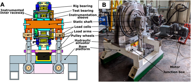
FIGURE 2. Cylindrical roller bearing test rig (A) schematic (B) photograph. Taken from Nicholas (2021).
The instrumented inner raceway, seen in Figure 3A is mounted onto a bearing carrier before being shaft mounted. The bearing carrier has a machined instrumentation slot
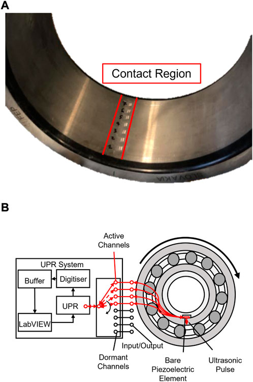
FIGURE 3. (A) Roller bearing inner raceway with a row of ultrasonic piezo elements instrumented on the inner, non-contact face (B) Schematic of ultrasonic pulser-receiver linked with instrumented bearings, adapted from Howard (2016)
2.2 Test lubricants
Two oils were used for testing, Alpha SP 320 and the less viscous Hyspin VG 32. Additionally, Mobil SHC 460 WT grease was tested. By using lubricants of different viscosities, densities and type (oil and grease) it was possible to investigate the potential to detect meniscus resonances and the effects on meniscus dimensions. Lubricant properties can be found in Table 1.
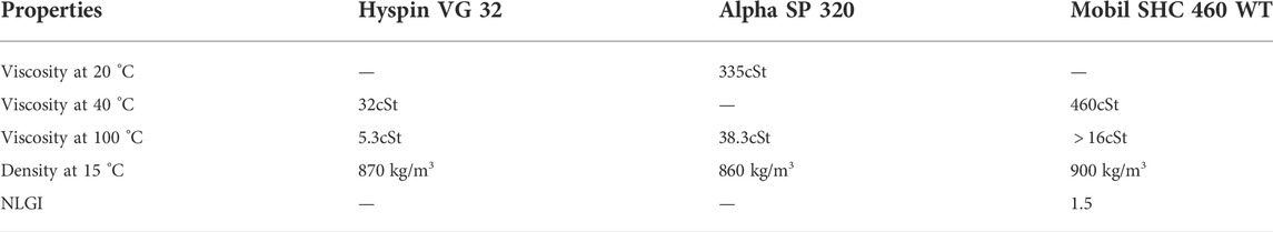
TABLE 1. Manufacturer stated properties of lubricating oils used for bearing test.
2.3 Ultrasonic test equipment
The ultrasonic test kit used was a personal computer with an in-built ultrasonic pulser receiver (UPR) to excite ultrasonic sensors, using a top-hat wave, and to record the reflections. The UPR can excite elements at a rate of 80 kHz known as the global pulse rate (GPR). The GPR is split over a possible 8 active channels and so if all channels are used, each channel pulse rate can be a maximum of 10 kHz. A digitiser records the reflected voltages at a rate of 100 MHz. Due to the high capture rate, a buffer is used to temporarily store recorded reflections before being permanently saved onto a hard drive. The UPR was controlled through a LabVIEW programme which allowed different pulse widths, delays, ranges and filters to be applied to each channel. This allows the user to optimise the excitation of the signal for the largest amplitude with the widest bandwidth. It also enables just the first reflection to be recorded which reduces data storage demands. Figure 3B shows a schematic of the UPR system linked up with the test bearing.
3 Experimental method
3.1 Bearing test methodology
Oil tests comprised of three 10 s captures at loads from unloaded to 500 kN in 100 kN increments, and five incremental speeds of 20–100 revolutions per minute, bearing speed n.dm of 6,200 to 31,000. By keeping test times short, the UPR can record at much higher pulse rates without filling the internal buffer and losing data. K-type thermocouples monitored oil supply and inner raceway temperature.
For grease testing, the added complexity of the churning phase Lugt (2013) was considered. Under a constant load of 400kN, 5 break-in stages were identified for the different bearing speeds. During these stages, lasting between 2 h and 5.5 h, the sensors were active (transmitting and recording reflections) for 5s followed by a 25s lay-off period. This allowed the UPR pulse rate to be high and comparable to the oil tests, without creating too much data which would limit the overall test time.
3.2 Reflection analysis
3.2.1 Sensor excitation and recording
As the bearing rotates, the UPR is used to sequentially excite all sensors linked to an active channel. For each UPR channel, the sensor is excited and the reflection recorded, before the next channel is excited. The channel pulse rate, Hz is user controlled, and dependent on the number of active channels and the length of capture. As csteel ∼ 6 km/s and the bearing raceway is only 19.5mm thick, it is a fair assumption that with a high channel pulse rate, different axial sensors are recording relatively the same roller radial position.
3.2.2 Live artificial reference from data mode
To interpret resonances due to a meniscus, it is necessary to obtain a reference signal where resonances are not present. Ideally, this is of a dry boundary or a film below the resonance range. This lubrication state naturally occurs outside of the contact and meniscus region, in-between rollers. Figure 4 shows how R changes as 4 rollers pass over the sensor location. Detail on how this plot is created is given in Section 4.1, but of note here is how the R = 1 across the majority of the plot, indicating from Eq. 1 there is a large acoustic mismatch. This occurs between steel-air, where no resonances are present. Therefore, for bearing referencing a live artificial reference was used, where the mode value for each data point within a signal, across a data capture, is used to artificially create a reference. More on this technique can be found by Howard (2016) and Nicholas et al. (2021). The benefits of this method are that it can be easily calculated in post-processing, and the reference is calculated at the same temperature as the actual measurement, so no complicated calibration is necessary.
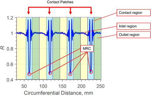
FIGURE 4. Schematic of the discretisation of the bearing pattern in the single frequency domain.
3.2.3 Measuring the resonant frequency
For every reflection captured, a specific series of data manipulation steps are taken to interpret the data. Figure 5A shows an oil reflection amplitude compared with that of an air reference from a validation test. The amplitude of the signal is reduced, due to wave transmission through the oil layer, and lengthened. The amplitude change is small, and according to Eq. 1 the sensitivity to the layer thickness is limited between 0.95 ≤ R ≤ 1, where R = 1 occurs with no oil present and R = 0.95 occurs when the oil layer is sufficiently larger than the wavelength. Therefore, further thickening of the film would not cause a monotonic decrease of R. Additionally, when the oil film is within the magnitude of the ultrasonic wavelength, R does not have a linear relationship with the thickness because of the interference in the oil layer, and so to determine thickness the signal must be analysed in the frequency domain.
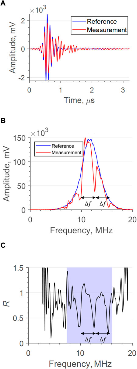
FIGURE 5. (A) Sample recorded reflections from an oil film and an air reference. (B) Reflections in the frequency domain. (C) Calculated reflection coefficient, for a sample signal from a validation test. The blue region again shows a typical usable bandwidth.
Initially, the signal is zero-padded to 2 × 10¹⁰ points long to reduce computation time and to increase resolution in the frequency domain. The signal then has a fast Fourier transform (FFT) applied, so that the signals can be manipulated in the frequency domain. Figure 5B shows the FFT applied to the measurement and reference signal. The amplitude reduction is again obvious, but it is noted that the reduction is not consistent across the entire bandwidth. Instead, the reduction is more severe at
However, as the acoustic mismatch between lubricant and solid is high, in some cases the majority of wave energy can be reflected at the first boundary and so the difference when compared with the reference is difficult to distinguish. Instead, the reflection coefficient can be used to assess these resonances. From the measured reflections, R is calculated as:
Where A(f) refers to the FFT amplitude and the subscript to the measured and reference signals respectively. Figure 5C is of the calculated R for a single reflection, and within the usable bandwidth highlighted in blue, there are clear resonant dips. During analysis, each reflection was analysed across a defined bandwidth within the frequency domain, in the following steps:
• First the Reflection coefficient was calculated from Eq. 12
• The R plots were inverted and a peak detection script was used to highlight resonances from the noise. As resonance amplitude can change with temperature, and the bearing naturally heats over the course of a test, constant peak parameters could not be used in the detection. Instead, all peaks within the frequency domain were recorded, and peak height and width were defined from the maximum peak detected, which corresponded with a resonant dip if present. A second detection pass was then used with the new peak criteria to eliminate noise and highlight only resonances.
• The isoutlier function in MATLAB was then used to filter out any large noise peaks, or “double dips” due to shearing motion, which were also observed by Pialucha et al. (1989).
• Finally, the number of resonances detected was limited between 2 and 10. This is done as at least 2 peaks are needed to calculate f0, as explained in Section 3.3, and if
• If a reflection has undetectable resonances due to either noise, a lack of oil film at the time of capture, or an oil film outside of the detectable range, a series of if functions deemed this a NaN value.
3.2.4 Calculating film thickness
An issue we found with having measurements only from the usable bandwidth is difficulties in knowing which order of resonance has been captured. For example, the first resonance captured is not necessarily f0 meaning that Eq. 11 is difficult to apply. However, if the bandwidth is large enough that at least two resonances are captured, the mean frequency difference between resonances
3.3 Measurement limitations, interval and uncertainty
The limits and precision of the resonance method are difficult to define as from Eq. 13 there is dependency not only on the frequency measurement, but also through the speed of sound value. The speed of sound is affected by several things such as temperature, pressure and aeration and so calculation of the measurement uncertainty of these parameters, which can be very difficult to measure in situ, should be estimated on a case-by-case basis. However, resonance detection is universal, regardless of the application.
For very thin films, f0 becomes increasingly large, as too does the required bandwidth to capture multiple resonances, and so only one resonance may be recorded. In this situation Chen et al. (2005) suggests that as no other resonances are detectable, the single resonance can be assumed to be f0. However, this does not hold true for all Bandwidths (BW). Take for example a typical bandwidth of a 10 MHz sensor between 5 MHz and 15 MHz. If f0 = 4 MHz, this resonance would not be detected, and only 3f0 = 12 MHz is within the bandwidth. If this was incorrectly assumed to be f0, the thickness measurement would be out by a factor of 1/3.
To address this issue, the authors propose two conditions in which either must be met to ensure a single observed resonance fr is the fundamental frequency and not a higher order odd harmonic:
If either condition is met, then it is assumed fr = f0. However, if the conditions cannot be satisfied, the assumption cannot be made, and at least 2 resonances must be recorded and
3.3.1 Minimum detectable film thickness
In all automated analysis completed the criteria in Eqs 14, 15 could not be met, meaning two resonances were required, and thus the lowest harmonics they could be were 3f0 and 5f0. The minimum detectable film thickness hmin therefore occurs when f0 is the highest it can possibly be while 3f0 and 5f0 are still within the bandwidth. This is when:
Where df is the frequency spatial resolution
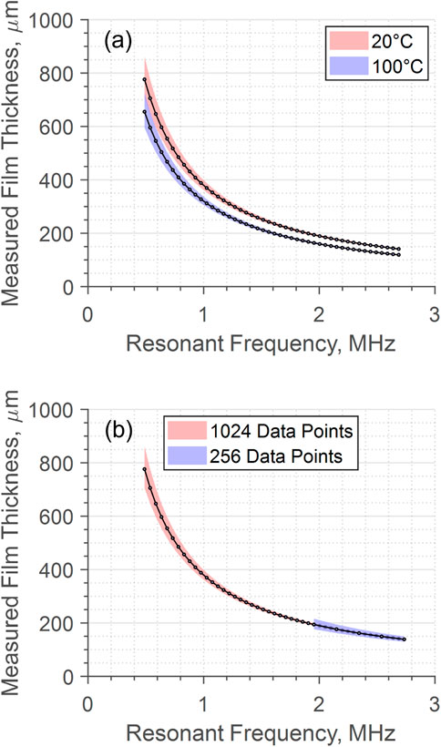
FIGURE 6. Comparison of measured thickness and interval with an increasing fundamental resonant frequency, with (A) two temperature extremes (B) different levels of signal padding at 20°C.
3.3.2 Maximum film thickness
The maximum detectable film thickness measurable using the resonance method is not as critical as there is an overlap with the TOF method. A thicker film corresponds with a lower fundamental frequency and therefore tightly banded resonances. Thus, the frequency discretisation determines the upper limit of film thickness hmax. For this work, 10 data points between resonant peaks were deemed an acceptable resolution, giving an adequate measurement interval for a thick film.
3.3.3 Measurement interval
The frequency spatial resolution is
The measurement interval can be improved upon by zero padding the recorded reflection before completing the FFT. This does not change the true resolution, but the interpolation allows for detection closer to the actual resonances. Figure 6B shows that by padding the signal further, the frequency resolution is improved, and so the measurement interval is decreased. Also, with the same criterium for the minimum number of data points between resonances, signal padding allows for the detection of thicker films as smaller frequency differences between resonances can be observed.
3.4 Resonant frequency—Thickness relationship validation
To validate that bare piezoelectric sensors could observe resonances in an oil film, the phenomenon was investigated on a simple spreading oil droplet. An aluminium plate, instrumented with a 10 MHz ultrasonic sensor and thermocouple, had droplets of different viscosity oils placed on the plate centre, corresponding with the sensor position, and were allowed to flow unhindered. Two Newtonian calibration oils were used for the experiment, Cannon S3 and the more viscous Cannon N10. Figure 7 shows a schematic of the test set-up. As the oil runs, the film thickness reduces, and so the layer measured becomes thinner over time. During the test, the sensor is continuously excited, to produce ultrasonic waves which interact with the oil layer, and then ‘listens’ for the reflections, in a pulse-echo configuration. The ultrasonic test equipment used was a compact low voltage version of the UPR kit used for the bearing test.

FIGURE 7. Schematic of the thinning oil droplet experiment.
Figure 8 plots (a) and (c) show reflection coefficient at a single frequency of
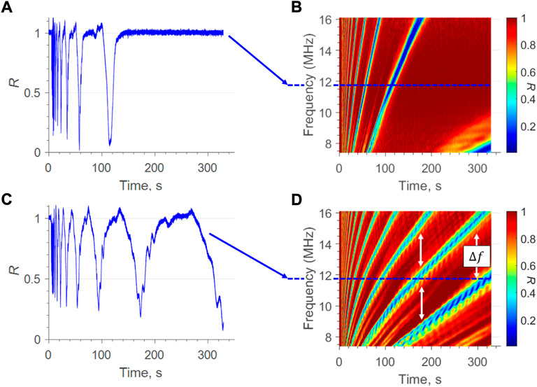
FIGURE 8. (A,C) single frequency analysis of s3 and n10 oils respectively. Plots (B,D) show the spectrogram oil map of the same oils.
Figure 9 shows the ultrasonic measurement of the thinning oil droplets for both viscosity oils. In the initial reflections, the oil droplet is thick and therefore measurable only by the well established TOF method. As the films continues to thin, reflections from the front and back face of the oil layer overlap and TOF becomes unusable, but the resonance technique is still applicable. for the less viscous s3 oil, the transition occurs at
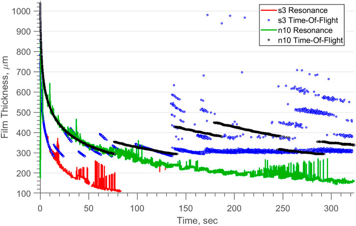
FIGURE 9. Film thickness of thinning oil drops measured by time-of-flight and resonance methods.
4 Results
4.1 Visualising the meniscus
Figure 4 shows the reflection coefficient, calculated from Eq. 12, change as 4 rollers pass over the piezo element location. Highlighted in blue is the contact region, and either side is the inlet and outlet meniscus, where there is a clear change from R = 1 to R ≈ 0.95 due to the presence of lubricant menisci. This type of plot shows the presence of a meniscus, but as sensitivity is limited between 1⪆R⪆0.95, the shape, length and thickness cannot be visualised.
Instead, a spectrogram similar to Figures 8B,D can be made by stacking together all the reflection plots, like those of Figure 4, at different bandwidth frequencies. Figure 10A shows an example spectrogram of a single roller contact with both an inlet and outlet menisci present, where the intensity of the plot is R. The intensity of the plot has been limited between 0.95 ≤ R ≤ 1.00 to improve the contrast around the resonant R values. 4 distinct areas are highlighted on the plot:
1. Red: outside the contact and meniscus regions where very little oil is present, and so no resonances can be seen here
2. Yellow: the inlet zone has horizontal dark fringes showing where the resonance occurs. Closer to the contact, the fringes become closer. This indicates that f0 is reducing, and thus the film is thickening into the contact.
3. Blue: this is the contact zone where there is a vertical, dark patch since the reflection coefficient is low. The oil is too thin to resonate here and so thickness measurements cannot be taken via resonance analysis. Thinner vertical lines also show evidence of interference within the entry and exit of the contact, due to complex reverberations within the bearing geometry Howard (2016). These interference fringes affect the resonant fringes of interest and so it is difficult to take film thickness measurements within this zone.
4. Green: this is the outlet meniscus region which, antithetical to the inlet region, shows horizontal fringes spreading. This indicates an increase in f0 and thus a film thinning towards the parched area between rollers.
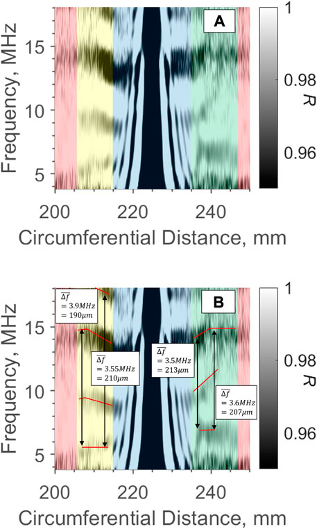
FIGURE 10. (A) Intensity plot of reflection coefficient spectrogram (B) same plot with estimated frequency value for indication of film thickness.
Figure 10B has drawn by eye resonances, and for single reflections
Of note is that the frequency jump between resonant minima is not always exact, as it is in theory, which is why it is important to calculate
4.2 Oil
Applying the detection approach of Section 3.2.3 to the resonant plots, Figure 11 shows the comparison between a single meniscus for VG 320 oil at Figure 11A 100 rpm and Figure 11B 40 rpm. For the majority of the measurement at both inlets there is a clear, consistent meniscus pattern. However, further away from the contact the pattern becomes much noisier, indicating the oil film in this region is below the minimum detectable threshold, but some noise peaks are still being detected causing the script to output a thickness value. Therefore, it can be assumed in these areas that the film is very thin in comparison with the measured menisci. Comparing cases a & b, the thickness values appear very similar, however the detectable menisci length at both inlet and outlet are shorter for the higher bearing speed case. Between the tests, there is a temperature change
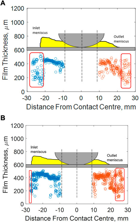
FIGURE 11. A comparison of contact entry and exit menisci thickness and length for a VG 320 oil lubricated bearing at (A) 100 rpm, n.dm = 31, 000 and (B) 40 rpm, n.dm = 12, 400.
Figure 12 shows a comparison of 2 inlet menisci recorded over a single 10s period. They seem to show two conflicting patterns, with a) being very thin and then growing into the inlet, and b) being thick and thinning into the inlet. Figure 12B is more representative of the norm for the test case. These results are taken from VG 320 oil at 20rpm and 500kN. Although the potential impact of either meniscus shape on the lubricating film is beyond the scope of this paper, clearly ultrasound has potential for detecting these changes if such an association were to be defined in the future.
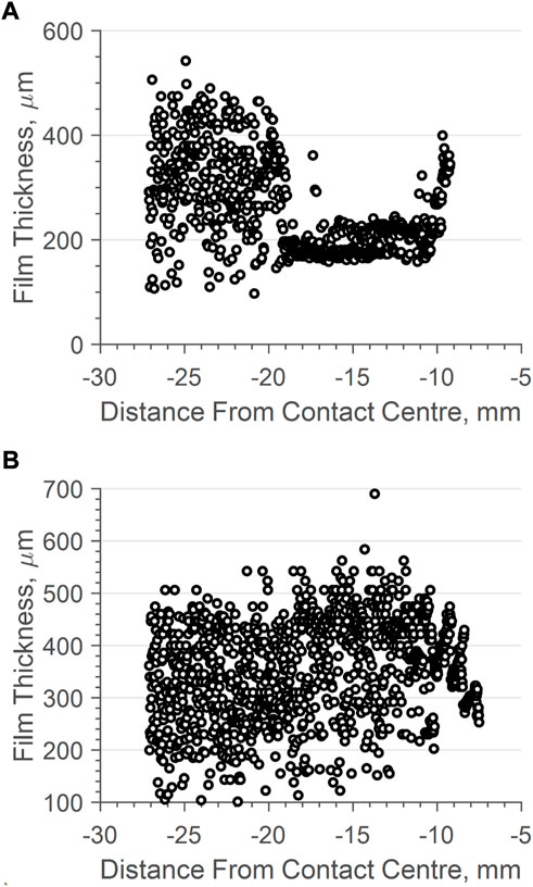
FIGURE 12. Inlet meniscus patterns for an oil lubricated bearing at 100 rpm (n.dm = 31, 000), 500 kN at (A) 10th roller pass (B) 19th roller pass.
Figure 13 shows a comparison of a single roller pass under the same bearing speed and load conditions, lubricated with VG 320 and VG 32 oil. The first order polynomial has been plotted for easier comparison. Although this is a comparison of just a single roller, it can be seen that the lower viscosity oil does not develop as thick a film at the contact inlet as the higher viscosity oil. Svoboda et al. (2013) found that thicker inlet films led to greater contact separation, and Crook (1961) found that contact film thickness increased with an increasing inlet viscosity. Figure 13 therefore suggests high viscosity oils create more separation in a contact by generating thicker films at the contact inlet.
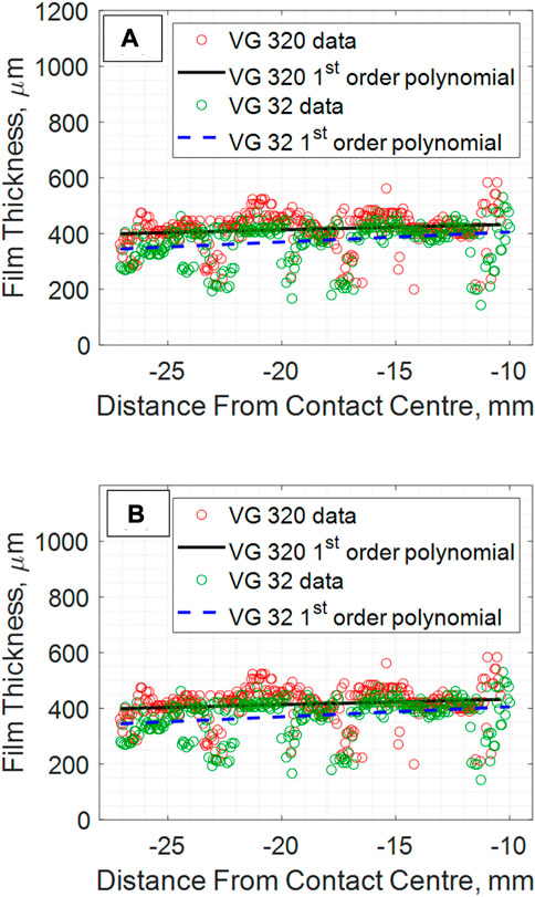
FIGURE 13. Meniscus patterns of a VG 320 and VG 32 oil lubricated bearing at the contact (A) Inlet (B) Outlet.
4.3 Grease
Ultrasonic measurements were taken for a grease lubricated case during the initial churning phase. During churning the fresh grease fibres are severely broken and the bearing begins to starve Lugt (2013). Figure 14 shows the meniscus shape change under constant load and speed, but captured at four different times after start-up during the churning phase. Observing from (a) to (d), as the grease is worked, there is a shortening of the meniscus length towards the contact inlet, which is associated with starvation, suggesting ultrasonic sensors can observe grease churn. In plot (d), which is at 58% of the total churn time, no meniscus is detected at the inlet and instead only noise is present. Again, this does not necessarily mean a meniscus is not present, only that if there, it is thinner than the minimum detectable value, around 290 μm for the grease tests.
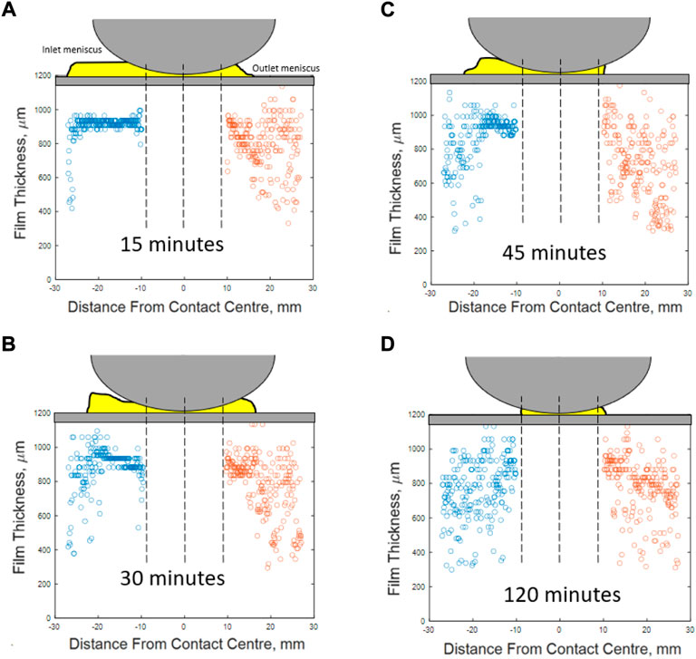
FIGURE 14. A comparison of contact entry and exit menisci thickness and length for 460 WT grease lubricated bearing after (A) 7% (B) 15% (C) 22% (D) 58% of the total churn time.
The outlet meniscus shows a similar pattern of shortening, and in (c) after 22% of the churn time, the outlet meniscus is not observed. However, in (d) at 58% of the churn time, an outlet meniscus is detected, suggesting that the meniscus recovery during churn is observable.
5 Discussion
From the previously presented results, bare piezoelectric ultrasonic sensors demonstrate the capability to cause resonance in lubricant films, at the entry and exit to a rolling element contact, and record the frequencies at which these resonances occur. Plotting the resonances as spectrograms allows a very easy inference of what the lubricant is doing during rotation:
• Fringes tightening shows a reduction in the f0 value, indicating a film thickening.
• Fringes spreading shows an increase in the f0 value, indicating a film thinning.
• Fringes with a constant resonant gap show a constant f0 value, indicating a film of consistent thickness.
Regardless of any further data analysis, these spectrograms by themselves have the potential to be a useful qualitative tool in first identifying the presence of a meniscus, and then inferring its growth/depletion.
The resonances are present in both oil and grease layers. This shows that both lubricant types are able to transmit an ultrasonic wave, and none of the lubricants tested had attenuation properties that made the resonance approach unusable. As both oil and grease have an acoustic impedance greater than that of air, resonances shown will always follow Eqs 8, 9. If the speed of sound through the lubricant is known, calculable from a simple calibration experiment, and the ultrasonic digitisation rate and bandwidth are large enough, then it is possible to calculate the film thickness.
This brings into question the thickness limitations of this resonance approach. Within this study, only longitudinal sensors with a central frequency of 10MHz were used, which obviously limits the bandwidth range, and measurable film thickness according to Section 3.3. However, it would be possible in future work to use a sensor pair of different central frequencies (e.g. 5 MHz and 10 MHz), and stitch the bandwidths together in post-processing to greatly increase the total bandwidth range. A single high frequency resonance could then be recorded, and it would be known to be f0 due to the lack of other resonances in the bandwidth if either conditions of Eq. 14 or Eq. 15 were met. Although this minimum thickness value varies depending on the speed of sound through the lubricant, it is feasible that films in the 20 μm range could be measured using such an approach. However, in this work we were limited to the use of 2 resonances, and so the minimum detectable film was 141 at 20°C and 119 at 100°C for oil, and 295 at 20°C and 290 at 100°C for grease.
The calculated film thickness is dependent on the measured frequency of resonances, but also on the speed of sound through the lubricant according to Eq. 13. One caveat to grease measurements is that the speed-of-sound calibration is performed on fresh, bulk grease. However, it is well established that during churning, oil is released from the grease. As speed of sound is a function of density, bled grease will have a different c value than fresh grease or oil. However, this discrepancy affects only the thickens calculation, not the length calculation that is dependent purely on resonance detection.
6 Conclusion
This work presents the novel application of an ultrasonic resonance method to growing and thinning lubricant films, which are in the sub mm range, and which occur at the entry and exit of rolling bearing contacts. When a lubricant film thickness is equal to a quarter of the ultrasonic wavelength interference between transmitting and reflecting waves in the oil layer cause a reduction in the recorded reflection amplitude, corresponding with a resonance. The frequency at which these resonances occur is therefore linked with film thickness. In the presented work, meniscus shape varies with changing bearing speed, lubricant type and at fixed locations, even with constant test conditions. Measured meniscus films were between
The future of this work is not just to observe changes in menisci length and thickness, but to quantify and understand how and why they differ. The importance of meniscus dimensions is noted in literature Wolveridge et al. (1970), as is the difficulty in measuring such a parameter. The presented work lays the foundation for a new approach that has the potential to take in situ meniscus measurements from operating bearings. This would be beneficial both for maintenance purposes, in detecting the early on-set of bearing starvation, and for investigating the fundamentals of oil and grease flow in test bearings without modifications that could alter the bearing kinematics.
Data availability statement
The datasets presented in this study can be found in online repositories. The names of the repository/repositories and accession number(s) can be found below: ORDA https://doi.org/10.15131/shef.data.c.6216734.v1.
Author contributions
WG performed the experiments, completed the data analysis and wrote the first draft of the manuscript. RSD-J provided expert guidance and intellectual direction during the course of the work. All authors contributed towards manuscript revision, and approved the final submitted manuscript.
Funding
The authors would like to acknowledge the financial support of the Timken Company who co-funded this work, and would also like to acknowledge the Engineering and Physical Sciences Research Council for funding through RDJ’s fellowship on Tribo-Acoustic Sensors EP/N016483/1 and the Centre for Doctoral Training in Integrated Tribology EP/L01629X/1. For the purpose of open access, the author has applied a Creative Commons Attribution (CC BY) licence to any Author Accepted Manuscript version arising.
Acknowledgments
The authors would like to thank Dr Benjamin Clark and Dr Gary Nicholas for help with instrumenting and assembling the test bearing. The authors would particularly like to acknowledge the help and advice of Dr Bill Hannon of Timken for his guidance throughout the work.
Conflict of interest
The authors declare that the research was conducted in the absence of any commercial or financial relationships that could be construed as a potential conflict of interest.
Publisher’s note
All claims expressed in this article are solely those of the authors and do not necessarily represent those of their affiliated organizations, or those of the publisher, the editors and the reviewers. Any product that may be evaluated in this article, or claim that may be made by its manufacturer, is not guaranteed or endorsed by the publisher.
References
Cameron, A., and Gohar, R. (1966). Theoretical and experimental studies of the oil film in lubricated point contact. Proc. R. Soc. Lond. Ser. A. Math. Phys. Sci. 291, 520–536. doi:10.1098/rspa.1966.0112
Cann, P., and Lubrecht, A. A. (1999). An analysis of the mechanisms of grease lubrication in rolling element bearings. Lubr. Sci. 11, 227–245. doi:10.1002/ls.3010110303
Cen, H., and Lugt, P. M. (2019). Film thickness in a grease lubricated ball bearing. Tribol. Int. 134, 26–35. doi:10.1016/j.triboint.2019.01.032
Cen, H., Lugt, P. M., and Morales-Espejel, G. (2014). On the film thickness of grease-lubricated contacts at low speeds. Tribol. Trans. 57, 668–678. doi:10.1080/10402004.2014.897781
Cen, H., and Lugt, P. M. (2020). Replenishment of the EHL contacts in a grease lubricated ball bearing. Tribol. Int. 146, 106064. doi:10.1016/j.triboint.2019.106064
Chen, Z. Q., Hermanson, J. C., Shear, M. A., and Pedersen, P. C. (2005). Ultrasonic monitoring of interfacial motion of condensing and non-condensing liquid films. Flow. Meas. Instrum. 16, 353–364. doi:10.1016/j.flowmeasinst.2005.06.002
Crook, A. W. (1961). The lubrication of rollers II . Film thickness with relation to viscosity and speed. Philos. Trans. R. Soc. Lond. 254, 223–236.
Dou, P., Jia, Y., Zheng, P., Wu, T., Yu, M., Reddyhoff, T., et al. (2022). Review of ultrasonic-based technology for oil film thickness measurement in lubrication. Tribol. Int. 165, 107290. doi:10.1016/j.triboint.2021.107290
Dowson, D., and Higginson, G. R. (1959). A numerical solution to the elasto-hydrodynamic problem. J. Mech. Eng. Sci. 1, 6–15. doi:10.1243/JMES_JOUR_1959_001_004_02
Dowson, D., and Toyoda, A. (1978). “A central film thickness formula for ehd line contacts,” in Proc. 5th leeds-lyon symp (London: Mechanical Engineering Publications).
Dwyer-Joyce, R., Drinkwater, B., and Donohoe, C. (2003). The measurement of lubricant- Film thickness using ultrasound. Proc. R. Soc. Lond. A 459, 957–976. doi:10.1098/rspa.2002.1018
Gomez Alvarez-Arenas, T. (2004). Acoustic impedance matching of piezoelectric transducers to the air. IEEE Trans. Ultrason. Ferroelectr. Freq. Control 51, 624–633.
Haines, N. F., Bell, J. C., and McIntyre, P. J. (1978). The application of broadband ultrasonic spectroscopy to the study of layered media. J. Acoust. Soc. Am. 64, 1645–1651. doi:10.1121/1.382131
Heemskerk, R. S., Vermeiren, K. N., and Dolfsma, H. (1982). Measurement of lubrication condition in rolling element bearings. A S L E Trans. 25, 519–527. doi:10.1080/05698198208983121
Howard, T. (2016). Development of a novel bearing concept for improved wind turbine gearbox reliability. Ph.D. thesis (Sheffield, England: University of Sheffield).
Kanja, J., Mills, R., Li, X., Brunskill, H., Hunter, A. K., and Dwyer-Joyce, R. S. (2021). Non-contact measurement of the thickness of a surface film using a superimposed ultrasonic standing wave. Ultrasonics 110, 106291. doi:10.1016/j.ultras.2020.106291
Kinsler, L. E., Frey, A. R., Coppens, A. B., and Sanders, S. V. (2000). Fundamentals of acoustics. New York, NY, USA: Wiley.
Kostal, D., Sperka, P., Svoboda, P., Krupka, I., and Hartl, M. (2017). Influence of lubricant inlet film thickness on elastohydrodynamically lubricated contact starvation. J. Tribol. 139, 1–6. doi:10.1115/1.4035777
Kumar, R., Kumar, P., and Gupta, M. (2010). Starvation effects in elasto-hydrodynamically lubricated line contacts. Int. J. Adv. Technol. 1. doi:10.4234/jjoffamilysociology.28.250
Lubrecht, A. A., Venner, C. H., and Colin, F. (2009). Film thickness calculation in elasto-hydrodynamic lubricated line and elliptical contacts: The Dowson, Higginson, Hamrock contribution. Proc. Institution Mech. Eng. Part J J. Eng. Tribol. 223, 511–515. doi:10.1243/13506501JET508
Lugt, P. (2013). Grease lubrication in rolling bearings. New York, NY, USA: John Wiley & Sons. doi:10.1201/b19033-24
Lugt, P. M. (2009). A review on grease lubrication in rolling bearings. Tribol. Trans. 52, 470–480. doi:10.1080/10402000802687940
Nicholas, G., Clarke, B. P., and Dwyer-Joyce, R. S. (2021). Detection of lubrication state in a field operational wind turbine gearbox bearing using ultrasonic reflectometry. Lubricants 9, 6–22. doi:10.3390/lubricants9010006
Nicholas, G. (2021). Development of novel ultrasonic monitoring techniques for improving the reliability of wind turbine gearboxes. PhD thesis (Sheffield, England: University of Sheffield).
Pialucha, T., Guyott, C. C., and Cawley, P. (1989). Amplitude spectrum method for the measurement of phase velocity. Ultrasonics 27, 270–279. doi:10.1016/0041-624X(89)90068-1
Schirru, M., Mills, R., Dwyer-Joyce, R., Smith, O., and Sutton, M. (2015). Viscosity measurement in a lubricant film using an ultrasonically resonating matching layer. Tribol. Lett. 60, 42–11. doi:10.1007/s11249-015-0619-x
Svoboda, P., Kostal, D., Krupka, I., and Hartl, M. (2013). Experimental study of starved EHL contacts based on thickness of oil layer in the contact inlet. Tribol. Int. 67, 140–145. doi:10.1016/j.triboint.2013.07.019
Wedeven, L. D., Evans, D., and Cameron, A. (1971). Optical analysis of ball bearing starvation. J. Tribol. 93, 349–361. doi:10.1115/1.3451591
Wilson, A. R. (1979). The relative thickness of grease and oil films in rolling bearings. Proc. Institution Mech. Eng. 193, 185–192. doi:10.1243/PIME_PROC_1979_193_019_02
Wolveridge, P. E., Baglin, K. P., and Archard, J. F. (1970). The starved lubrication of cylinders in line contact. Proc. Institution Mech. Eng. 185, 1159–1169. doi:10.1243/pime_proc_1970_185_126_02
Keywords: EHL, meniscus, grease, oil, lubrication, rolling bearings
Citation: Gray WA and Dwyer-Joyce RS (2022) In-situ measurement of the meniscus at the entry and exit of grease and oil lubricated rolling bearing contacts. Front. Mech. Eng 8:1056950. doi: 10.3389/fmech.2022.1056950
Received: 29 September 2022; Accepted: 26 October 2022;
Published: 07 November 2022.
Edited by:
Hui Cen, Xuchang University, ChinaReviewed by:
Tonghai Wu, Xi’an Jiaotong University, ChinaWenzhong Wang, Beijing Institute of Technology, China
Copyright © 2022 Gray and Dwyer-Joyce. This is an open-access article distributed under the terms of the Creative Commons Attribution License (CC BY). The use, distribution or reproduction in other forums is permitted, provided the original author(s) and the copyright owner(s) are credited and that the original publication in this journal is cited, in accordance with accepted academic practice. No use, distribution or reproduction is permitted which does not comply with these terms.
*Correspondence: W. A. Gray, d2FncmF5MUBzaGVmZmllbGQuYWMudWs=