1
Institute of Cognitive Science, Department of Neurobiopsychology, University of Osnabrück, Osnabrück, Germany
2
Department of Neurophysiology and Pathophysiology, University Medical Center Hamburg-Eppendorf, Hamburg, Germany
Here we introduce a cognitive model capable to model a variety of behavioral domains and apply it to a navigational task. We used place cells as sensory representation, such that the cells’ place fields divided the environment into discrete states. The robot learns knowledge of the environment by memorizing the sensory outcome of its motor actions. This is composed of a central process, learning the probability of state-to-state transitions by motor actions and a distal processing routine, learning the extent to which these state-to-state transitions are caused by sensory-driven reflex behavior (obstacle avoidance). Navigational decision making integrates central and distal learned environmental knowledge to select an action that leads to a goal state. Differentiating distal and central processing increases the behavioral accuracy of the selected actions and the ability of behavioral adaptation to a changed environment. We propose that the system can canonically be expanded to model other behaviors, using alternative definitions of states and actions. The emphasis of this paper is to test this general cognitive model on a robot in a real-world environment.
An increasing number of studies model animal behavior using robots. While many of these studies investigate how individual components, such as sensory processing, contribute to the generation of behavior (Lungarella et al., 2003
), most are limited to modeling one particular behavioral domain (Alexander and Sporns, 2002
; Edelman, 2007
). It is becoming more and more obvious that the flexibility of human behavior is still out of reach of modeling studies (Flash and Sejnowski, 2001
; Todorov, 2004
). Recently in the neurosciences, different approaches have delineated behavior in a unified theory, independent of any specific paradigm (Wolpert and Ghahramani, 2000
; Schaal and Schweighofer, 2005
). Here we develop a model based on general principles that we propose to generalize over a broad variety of behavioral domains.
For the present study we apply and test the cognitive model in the domain of a navigational task. Navigation refers to the practice and skill of animals as well as humans in finding their way and in moving from one place to another by any means (Wilson and Keil, 1999
). Hence, a navigational task can be described computationally by referring to the position and orientation of the agent as a function of time. Furthermore, the ability of animals to navigate in 2D environments like the four-arm maze has been studied extensively (Olton and Samuelson, 1976
; Morris, 1984
). To test the cognitive architecture we thus chose an easily determinable navigational task based in the standard environment of a four-arm maze.
To perform a planned behavior, a robot has to predict the sensory outcome of its actions. In order to do so, it is useful to reorganize the high-dimensional sensory input into a low dimensional representation consisting only of behaviorally relevant aspects. Several studies (Wyss et al., 2006
; Franzius et al., 2007
) have recently shown that place cells can be understood as the result of an unsupervised learning procedure applied to the visual input of a behaving robot. In these studies the weights between units in a hierarchical neural network are adjusted, such that the firing rate changes as slowly as possible with time. The resulting activity patterns thus form an optimally stable representation of the sensory input. The results of learning in these hierarchical networks match the experimental observations of place cells as found in rodent hippocampus (O’Keefe and Dostrovsky, 1971
). These neurons fire only when the animal is located in a certain region of the environment, defining the cell’s place field. Although the contribution of these cells to the animal’s behavior has still not been fully understood, it is assumed that these cells constitute a cognitive map of the environment (O’Keefe and Nadel, 1978
) and serve as the basis of navigation. The work of Wyss et al. (2006)
implies that unsupervised learning of the sensory input results in a reorganization of the sensory space, originally spanned by its visual input to a spatial interpretation. We built on this research by using place cells to represent the location a robot in its environment. Thus the place fields constitute a discretization of the navigational state space spanned by the robot’s position. They correspond to the robot’s internal states and represent the positions it can differentiate. In summary, in order to enable the cognitive model controlling the robot to navigate, we chose place cells as a biologically plausible and theoretically founded representation of the environment.
An important aspect of the proposed model is the division of the architecture of the agent into central and distal processing. Both processes learn the sensory outcome of the robot’s actions in the agent’s state space, spanned by the place fields. The central processing component captures the sensory outcomes of the agent’s actions. It is defined by the state (place field), where the robot is located after the execution of the action. Exploratory behavior leads to learning which action leads to a specific outcome. The agent stores experienced state transitions as transition probabilities. In contrast, the distal component is based on infrared sensors and accounts for reflexive behavior. Triggered reflexes are memorized as so-called reflex factors. These facilitate obstacle avoidance only, and are not used to constitute the robot’s state. Combined, transition probabilities and reflex factors reflect the environmental properties in relation to the robot’s actions.
Based on exploratory behavior the robot learns an approximation of the environmental affordances (Gibson, 1977
) for navigation, defined as the navigational action possibilities afforded by the environment. The cognitive model plans goal-directed actions by integrating the information gained by central and distal processing into a local decision-making process. This integration results in a quantitative measure of how reliably each executable action leads towards the goal. Hence, the key components of our cognitive model are (i) a high-level representation (place fields) of sensory input space, (ii) the knowledge of environmental properties acquired by active exploration of local state transitions by means of distal and central processing and (iii) a decision-making process driven by this knowledge.
Here we show that using the described cognitive model the agent latently learned the environmental affordances and let a robot successfully navigate to different goals within a four-arm maze environment. Importantly, the differentiation between central and distal processing reduces the negative effect of the obstacle-avoidance behavior on navigational performance, and enables the robot to quickly adapt to changes in the environment. We propose that by redefining the states and actions, the introduced model can be expanded to model other types of behavior.
Overview of the Architecture
Our cognitive model allows the robot to explore the environment and navigate to different targets based on a state space represented by the spatial representation of place fields. This state space was obtained by dividing the four-arm-maze environment (Figure 1
A) into compact, discrete states (Figure 1
B), similar to the place fields that can be acquired by unsupervised learning (Wyss et al., 2006
). The central component of the model processed every one of the robot’s state transitions, while the distal component dealt only with transitions that coincided with reflexive behavior (obstacle avoidance). Together, the transitions induced by the robot’s actions and those transitions associated with reflexive behavior represent the environmental properties locally learned by the exploring robot. During each stage of the decision-making process, the model chose the action that maximally increased the probability of reaching a desired target within the environment, thus allowing the robot to successfully navigate.
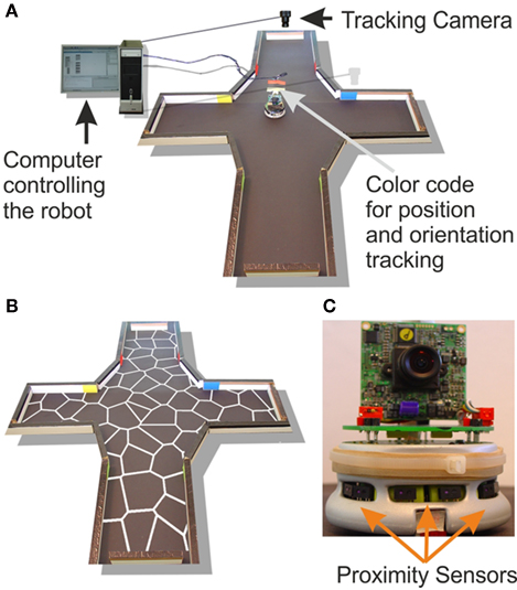
Figure 1. (A) A four-arm-maze environment was chosen to test the model. A Khepra robot was controlled by an agent implemented in the MicroPsi framework, running on a computer. The inputs to the program were the orientation and the position of the robot, as well as the data from the proximity sensors. (B) shows the distributions of states used. The white lines within the environment represent the boundaries of these states. (C) shows these proximity sensors on the robot. These sensors emit infrared light and measure the reflection. The agent used the activation of the place cells which corresponded to its current position, the orientation of the robot, and the proximity sensors to perform the robot’s behavior.
Place Field Representation
We chose place cells as a representation of the environment. A study by Wyss et al. (2006
) showed that such place cell properties can be acquired by mobile robots by means of unsupervised learning in a hierarchical network. Although it would be possible to replicate this work, our main purpose here was to model behavior, so we deliberately used predefined place cells, similar in type to those observed in the previous study, to focus on the behavioral aspect. We approximated the firing properties of place cells as a function of the robot’s position by 2D Gaussian functions (standard deviation: 0.04 m). To cover the whole four-arm-maze environment we randomly distributed 72 of these Gaussian functions (Figure 1
B). For each of the robot’s possible positions within the maze, we obtained the activity of each of these place cells. A winner-takes-all process then extracted the robot’s position in state space from the population activity of the place cells – the cell that was maximally active thus defined the current state of the agent. In order to calculate the place cell activity, we first needed to extract its position in the environment. The robot was tracked by an Analog Camera (Color Cmos Camera 905C) which was attached above the environment as shown in Figure 1
A. The analog camera signal was digitized by a TV card (Hauppauge WinTV Express). The position and orientation of the robot were then calculated using the camera image and the color code attached on top of the robot. Thus, the population of place cells represented a mapping from the position space in which the robot was navigating, to the state space of the agent controlling the robot. To secure generalizability, no reference was made to the 2D structure of the environment. The only information used by the agent to infer the robot’s position was the activation of each place cell.
Action Execution
In order to limit the number of transitions needed to learn the environmental properties to a manageable number, in each state the robot was restricted to executing eight different actions. Each of these actions consisted of a static rotation to a certain global orientation followed by a straight-line movement of the robot. The corresponding orientations were equally spaced from 0 to 325°. As a result of executing such an action when in a given state (source), the robot will reach a different state (endstate), with the action thus resulting in a transition between states. An endstate was reached when the winner-take-all process calculating the current state returns a new state index. A transition was defined as complete when a local maximum of the endstate’s activity was reached. A local maximum occurred when the derivative of the current state’s activity becomes negative. The frequencies of the transitions resulting from action i, executed in source state j and ending in endstate k were stored in the experience matrix EMi,j,k..
Distal Processing
To prevent the robot hitting one of the maze’s boundary walls, a reflexive obstacle avoidance behavior was implemented. The proximity sensors (Figure 1
C) were used to perform this behavior, such that we directly mapped the inverse activities of the sensors to the motor activity. The sensors at the side of the robot reduced the motor activity, sent to the wheel located at the same side and reduced it for the wheel at the opposite side. The frontal sensors both reduced the motor activity sent to both wheels. In both cases a negative motor activation was possible such that the wheel rotated in the opposite direction compared to a positive motor activation. The frequencies of occurrence of the reflexive event characterized by the particular state (i) – action (j) combination was stored in the reflex matrix RMi,j. Whenever the robot used its obstacle avoidance behavior, the system associated the current state and action with the occurrence of a reflex event and updates the reflex matrix accordingly.
Decision Making
Here we addressed the problem of decision-making – choosing the action that is most likely and quickest to lead towards the goal. As the obstacle avoidance behavior introduced additional variability in state transitions (see Results), the agent should also minimize the usage of this behavior during his movement to the goal. In this section we developed a measure for each action on each state resulting from an iterative reverse flooding procedures Figure 2
defining the actions likeliness and quickness to lead to the goal.
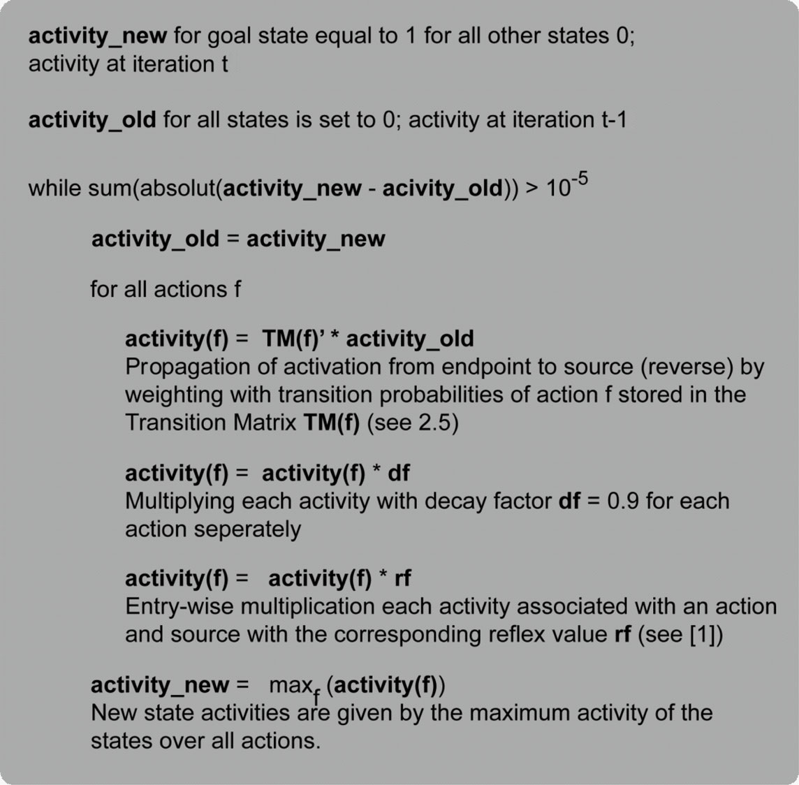
Figure 2. Description of the reverse flooding algorithm.
The reverse flooding procedure integrated the transition probabilities experienced by the agent to evaluate the probability to end up at the goal state. The transition probabilities were learned by the central component of the model and were stored in a transition matrix (Figure 3
A). The transition probability defined by source j, endstate k and action i was stored in the transition matrix TMi,j,k shown in Figure 3
A. The sum of the transition matrix over the endstates k (rows) was normalized to one for each action and source and thus represented a probability distribution. The 3D transition matrix consisted of eight 2D matrices, each for one action i TMi. These eight transition matrices TMi shared some similarity with a directed graph. The vertices of this graph corresponded to the states, the edges corresponded to the transitions, and the edge weights to the transition probabilities. This results in eight directed graphs equivalent to the eight possible actions. In each of the iteration steps of reverse flooding, the activation of the state corresponding to the goal state was set to one. State activation was propagated through the graph by passing the activity – weighted by the corresponding transition probability – to connected states in the reverse direction of the directed edges. Technically speaking, the activation was propagated from endstates to sources, weighted by the transition probability of the action’s transfer from the source to the endstate, hence the name reverse flooding. Applying this process to each action’s graph gave rise to eight different activity values for each state. These activity values were proportional to the probability to reach the goal by executing the corresponding action on each state. Up to this point, only the learned environmental properties resulting from central processing were considered during flooding.
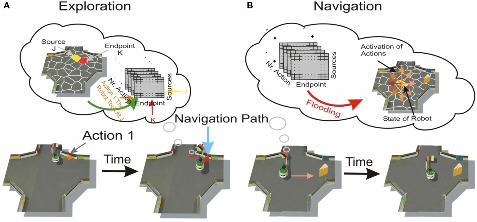
Figure 3. (A) Learning of the properties of the environment. The robot is on a certain state, defined here as Source J (yellow labeled) and randomly chooses an action (Action 1). The execution of the action results in another state, defined as endstate K (red labeled). This transition was stored in a 3D matrix, called the experience matrix, with the dimensions sources, endpoints and actions. The number of action executions combined with obstacle avoidance from a source was stored separately. (B) The robot moving to a goal (the “cheese” for the artifical “rodent”). His choice is a consequence of the flooding of the transition matrix, resulting in an activation of the different actions, shown as colored arrows. The action with the strongest activation was chosen.
Further to minimize the number of reflexive events during navigation to the goal, we integrated the distal component in the flooding procedure. This was done by introducing reflex factors. The reflex factor was proportional to the percentage of actions i at source j that induced reflexive event:
During each iteration step, the eight activations of state j corresponding each to one of the eight actions i were multiplied by the corresponding reflex factor rfi,j. The maximum of the eight activations of a state was used as the state’s activation for the next iteration step. These eight activations were generated by multiplying the activity by the transition probabilities and the reflex factor, both smaller or equal to one. Thus each of those eight activation was smaller or equal to one. Applying the maximum operation to these eight activation of a state to define the state’s activation for the next iteration step, restricted the activity of a state to be smaller or equal to one. Thus, for the flooding procedure we did not apply any additive process to the activation propagation, which restricted the state’s activity to be equal or smaller than one. Further, by injecting in each of the iteration steps an activity of one at the goal state, the flooding procedure resulted in a steady-state of state’s activity. Thus, this iterative flooding process was continued until the states’ activities converged. In order to select the action most likely to move the robot towards the goal, we considered the eight incoming activation values on each state, which resulted from the activation propagation of the eight actions. The robot then chose the action corresponding to the highest incoming activation of the current state to move to the goal (Figure 3
B).
For the reflex factors we introduced a weighting factor of 5/6 to prevent a reflex factor of zero in the case of an action, which was combined only with obstacle avoidance behavior. Thus, non-zero reflex factors did not neglect the information of the environment gained by the transition probabilities during the flooding process.
Furthermore, to reduce the number of transitions to move to the goal, we introduced a decay factor df, which was here set to 0.9. After each iteration step, the activation of each state was multiplied by this factor. The more transitions that were needed to reach the goal states, the more the decay factor was taken into account and decreases the states’ activities. Hence, the decay factor penalized longer trajectories to the goal state.
The flooding algorithm defined above was implemented with the help of matrices.
represented the activation at the 0’th activation propagation, where the goal was located at state m.

where  was the vector of activation values for the states after t iteration steps. rf represented the reflex factor and df the decay factor. After the convergence of the activities, the index i with maximal activity of a state define the action that is chosen by the agent to navigate to the goal. The convergence of the activities was defined by the absolute difference between previous and current activities being smaller than 10-5.
was the vector of activation values for the states after t iteration steps. rf represented the reflex factor and df the decay factor. After the convergence of the activities, the index i with maximal activity of a state define the action that is chosen by the agent to navigate to the goal. The convergence of the activities was defined by the absolute difference between previous and current activities being smaller than 10-5.Robot Setup
To test the model in a real-world environment we used Khepera II robots (K-Team, Lausanne, Switzerland). The robot was equipped with eight proximity sensors, which emitted infrared light and measured the strength of its reflection. Propulsion is achieved by two wheels, each controlled by a separate motor (Figure 1
C). For implementation and flexible programming, we used MicroPsi (Bach, 2003
; Bach and Vuine, 2003
), an Eclipse-based Java programming environment, as an interface to the robot. The agent that controlled the robot’s behavior was implemented in this framework. The particular cognitive model was implemented with the help of the Colt framework, allowing matrix calculation in Java. The real-world environment was a four-arm maze with boundaries built from white wooden pieces (Figure 1
B). Each arm had a width of 0.21 m and a length of 0.28 m. The four-arm maze environment fitted into an area of 1 m2.
Analysis
As a means of comparison, a simulated robot was implemented in MATLAB (Version 7.0 (R14), Mathworks, Natick, MA, USA) using the same algorithms described above. Obstacle avoidance behavior of the physical robot was approximated setting the angle of reflection equal to the angle of incidence to the boundary, with a random scatter of 10 to −10 degrees added.
To compare the navigational behavior and the transition probabilities learned by the robot, we introduced the geometrical transition matrix. This matrix took into account only the topographical properties of states in the environment and was created by allowing the simulated robot to execute every action on every position within each state, using the resolution of the camera tracking system. Because the real-world robot chose a new action only at a local maximum of its current place cell activity, each transition occurrence in the simulated agent was weighted by the probability of the robot executing an action given the current place cell activity. In an ideal world and given a very long exploration time the real transition matrix was expected to converge to the geometrical transition matrix. In the real-world setup, due to the finite robot size, slip and friction and a limited exploration time, the geometrical transition matrix might deviate considerable from the real transition matrix.
Next we evaluated the properties of the experienced and geometrical transition matrices. First we investigated the similarity of action outcomes by comparing the corresponding transition probabilities. We correlated the transition probabilities represented by a row vector of the Transition matrix of action i, TMi, with the same row vector of the Transition matrix of action j TMj. Before calculating the correlation coefficients between the two vectors we reduced the transition probabilities in the row vector by the average of these transition probabilities to the topographical next neighbors. Thus two actions led to equivalent outcomes when their correlation coefficient is 1.0; they are linearly uncorrelated when the correlation coefficient is 0.0.
We characterized the predictability of an actions’ transition to a state by defining a second measure: The predictability of action i in state j is given by the maximum transition probability stored in the row vector j of the Transition Matrix TMi. This maximum transition probability was reduced by the probability of transferring to one of the connected states by chance.
Here, Pri,j corresponded to the predictability of action i in state j, and conni,j is the number of states the robot was able to reach by executing action i on state j.
In order to evaluate the decision-making process, we analyzed the activation of each action after the flooding process had converged. We chose the normalized activity as an appropriate measure to characterize the quality of selection of an action during navigation to a goal. This normalized activity is defined as the activation of the chosen action j for the state, normalized by the sum of all incoming activity and by the decay factor.
with actj representing the maximum converged activity of state j after flooding. The denominator corresponded to the sum of all converged incoming activations of state j for all actions. In order to reduce the dependency of the normalized activation on the decay factor, we included the decay factor in the denominator. As a result of its inclusion, the normalized activity ranged from 0 to 10. The value of 10 is reached when only action j has an activity and thus all other actions are not activated. This indicated, that only action j is leading the robot reliable to the goal. While smaller values of the normalized activity represented similar activation of all actions, and thus executing one of the other action could lead the robot to the goal with a similar navigational performance. Thus, as smaller the normalized activity values as similar are the activations and thus any action will lead the robot to the goal.
Batch and Online Learning
We investigated the plasticity of the introduced navigational system by examining the robot’s navigational adaptation to changes in the environment. The robot’s navigational performance was evaluated by measuring its navigational performance to a target. We examined the robot’s adaptation process by comparison of the two different types of learning we introduced: batch and online learning. These approaches differed in the timing of the transition matrix and reflex update and in the way in which the robot explored the environment. Batch learning involved interleaved experience stages of random action execution, during which the existing transition and reflex matrices were updated, and evaluation stages, during which navigation took place and the transition and reflex matrices were not updated. This is similar to the way the agent experienced the environment as described above. In comparison, online learning involved updating the robot’s transition probabilities and reflexes after each action execution, and instead of moving randomly, the decision-making process was always at work.
Here we investigated the robot’s navigational performance and how the central processes – namely the transition probabilities – as well as the distal processes defined by the reflex factors, contributed to the decision-making process. We also examined the adaptation of the robot’s navigational behavior to changes in the environment.
Navigation Behavior
Navigational performance
The navigation performance of the robot was evaluated by repeatedly measuring its path to a number of different target sites in the environment. In each of the 20 trials, the robot was placed on one of five possible starting positions and given one of four target locations. In order to directly compare different start-target combinations, we normalized the length of the robot’s path by the direct path, which represented the shortest traversable distance from the robot’s starting point to the goal state. Figure 4
shows a path traveled by the robot (yellow line) and the corresponding direct path (light gray line). Overall, the robot’s median path length across 20 trials was 1.71, with a standard deviation of 0.47. This represents an increase of 71% (±47%) compared to the direct path length. For all configurations of start positions and targets, the robot was able to reach the target in a reasonably short amount of time.
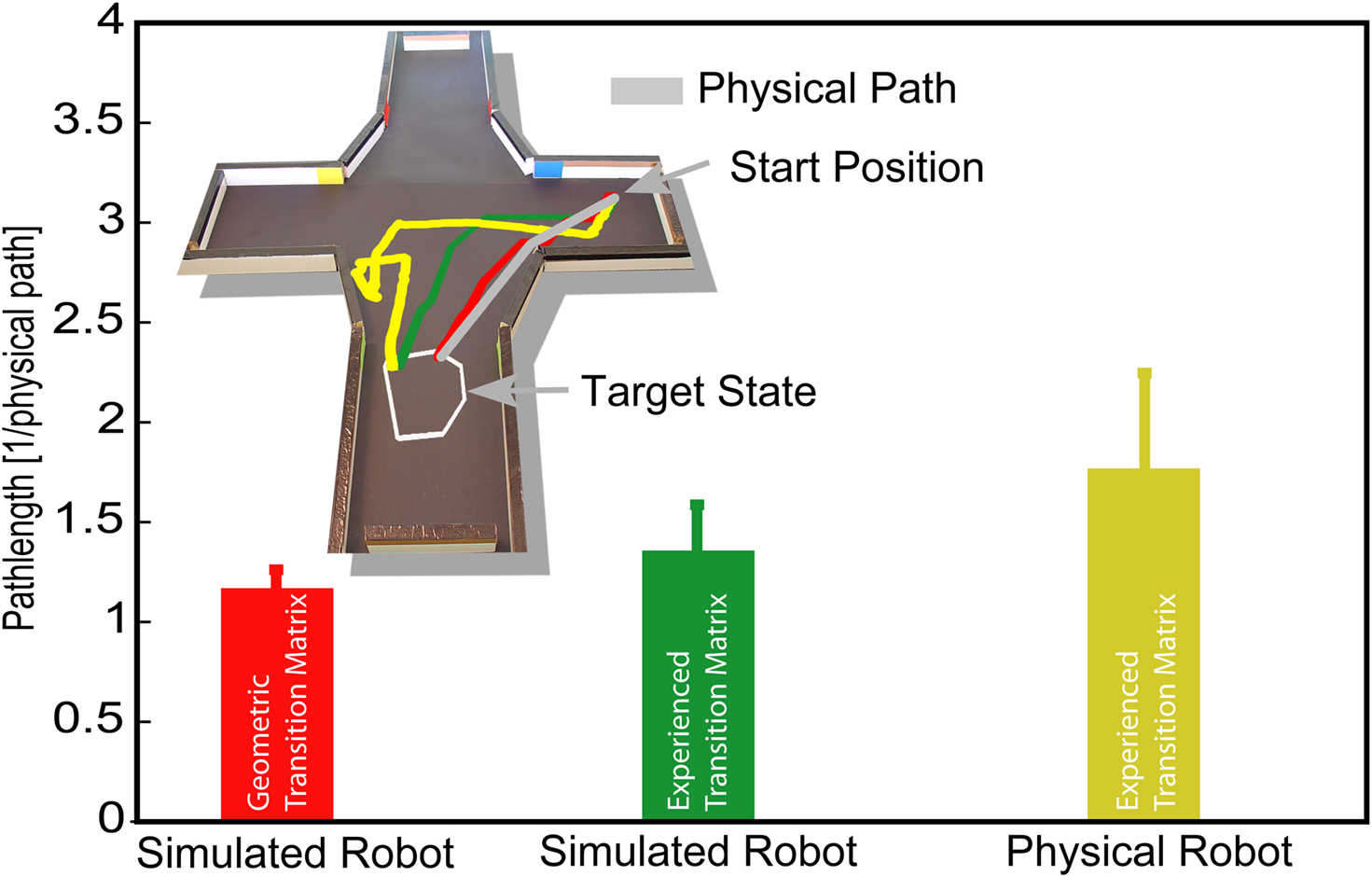
Figure 4. Navigational behavior of the robot was investigated by measuring the length of the path to different goals. The direct path, defined as the shortest traversable path from the start point to the goal state (shown as the gray line in the upper part), was used to normalize the length of the robot’s path (yellow line) to the goal. The red line corresponds to the length of a path of a simulated robot by taking the topographical distribution of states (geometric transition matrix) into account. The bars represent the median length between different starting and goal states and their standard deviation.
Impact of states and learned properties on navigational performance
The increased length of the robot’s paths could be a consequence of any of the following: the division of the environment into discrete states (place fields), the environmental properties learned by the robot (transitions and reflex factors), and the robot’s behavior while navigating through the environment. Each of these factors was investigated in turn. To provide a first approximation of the increase due to the discretization of the environment, we simulated the robot’s behavior using the same navigational algorithm as described in the Section “Materials and Methods”. The simulation used the geometrical transition matrix, which takes only the topography of states into account (see Materials and Methods), to navigate from the same start positions to the same goal states as the real robot. The red line in Figure 4
shows a sample path of the simulated robot. This simulation resulted in a median increase of 19% (±9%) compared to the direct path. Thus, the introduction of discrete states did not greatly contribute to the lengthening of the robot’s path to a goal.
Additionally we investigated the influence of the size of the states on the navigational performance. Because of the spatial extension of states, the robot chose an action in order to navigate to the goal at from different positions within a state. Thus, the robot was able to chose at an action in order to move to the goal at different positions within a state at different positions than the robot experienced the transition probabilities. Do these different positions have an impact on the robot’s navigational performance? In order to solve this question we let the simulated robot start from different position within a state and let him navigate to a certain goal by utilizing the real robot’s experience matrix and reflex matrix. This procedure was done for 12 start states to each of 12 goal states within the arena. We hereby distributed the start position equally over the spatial extension of the state and measure the length of the path from the start position to one of the goal states. This length of the path was normalized by the length of the path from the center of the Gaussian activity function of the corresponding state (place field) to the goal state. In case the simulated robot had not to navigate around the corner, the mean ratio of the traveled path to the one from the center of a Gaussian activity was 1.016 (±0.123), while for cases the robot had to navigate around the corner a mean normalized path of 1.138 (±0.137) was measured. Thus only a small variation of the navigational performance caused by the spatial extension of states was obtained. In case the robot has to navigate around the corner, the spatial extension of states has a higher impact of the navigational performance. Further, as described in the Section “Materials and Methods”, the robot only chose an action at positions within a state, which are associated with the first occurrence of a negative activity gradient on the robot’s path. This region of possible positions was defined by analyzing the positions the real robot chose an action. By distributing the start position in each of the 12 start states equally in this regions of possible positions we evaluated the navigational performance of the simulated robot to each of 12 goal states. The mean ratio of the robots path to the one from the center of the Gaussian activity was 1.022 (±0.065) with the robot navigating around the corner, while without a corner a mean normalized path was 1.017 (±0.055). In case the robot has to navigate around the corner, the state’s spatial extension has a higher impact on the navigational performance. In both cases of navigation, the impact on the navigational performance is small. In summary, the spatial extension of states has only a small impact on the navigational performance.
Next we investigated the contribution of the robot’s learned environmental properties. To do so, we again used the simulated robot with the same start-target combinations, but this time used the robot’s learned transition matrix and reflex factors to perform the task. Figure 4
shows an example of such a simulated path (green line). The median increase in path length was 37% (±23%). As 19% of the path increase is caused by discrete states, approximately 18% is due to differences between the geometrical properties of the environment and those properties learned by the robot. Thus, the difference between the geometric and learned transition matrices and reflexes explains a further quarter of the lengthening of the path of the real robot while navigating to a goal. Again, this is a small contribution to the overall increase of the path length.
Summary
How can we interpret the robot’s navigational behavior? Approximately a quarter of the increase of the robot’s path to a goal was due to the representation of the environment by discrete states of finite size. Another quarter of the lengthening was explained by the differences between the geometrical properties of the environment and those learned by the robot. We also analyzed the effect of obstacle avoidance on the robot’s performance. The agent engaged its obstacle avoidance behavior in 60% of the trials, independent of the particular combination of start and goal states. Analyzing only the trials in which the agent did not engage obstacle avoidance, we obtained a median path length of 1.36 (±0.23), which was similar to the length measured in simulation with the transition matrix learned by the real-world robot. This was due to operational differences – particularly in obstacle avoidance behavior – between the robot and the simulation (see Materials and Methods). Thus the median path length given by the robot’s learned transitions represented an approximation of the contribution of obstacle-free navigation. Consequently, the largest share of the lengthening of the robot’s path compared to the direct path was due to the obstacle avoidance behavior, which was usually triggered when the robot moved through the narrow arms of the maze. In all configurations of goal states and start positions, the robot was able to find its goal in a reasonably short amount of time, with the main increase in path length arising from obstacle avoidance behavior.
Analysis of the Central Component
The robot’s performance in this navigation task was a direct result of the underlying decision-making process. This process was based on the learned transition and reflex factors, which represent the learned environmental properties. Here we investigated the characteristics of the robot’s learned transitions by looking at: (i) the differences between the transitions of different actions on a state, (ii) the influence of the used topographical distribution of states on the learned transitions of, (iii) the number of different states reachable by the different actions, (iv) the predictability of the state reachable by a single action execution, and (v) the effect of the robot’s limited learning time on the learned transition probabilities. For the most part, we analyzed the characteristics of the transition matrices by comparison to the simulation based on the geometrical transition matrix (see Materials and Methods), which only took the used topographical distribution of states into account. This comparison allowed us to investigate the extent to which the topographical distribution of states gave rise to the investigated characteristics of the transition matrix.
Properties of learned transition probabilities
Here we analyzed the similarity between the transitions of different actions, defined as the redundancy of the robot’s possible actions on a state, by comparing the transition probabilities associated with these actions. For this purpose we computed correlation coefficients (see Materials and Methods and Figures 5
A,D) between the transition probabilities of the different actions on each state. Higher correlation coefficients (>0.5) were more frequently observed in the experienced transition matrix (44%) than in the geometrical case (25%), (Figure 5
A). Thus, the robot’s real-world action execution resulted in more similar outcomes and a higher redundancy of the actions, as compared to the geometrical case. Most (93%) of the highly correlated actions in the experienced case were obtained for states at the boundaries of the environment, and so were primarily due to the obstacle avoidance behavior elicited by wall contact. Overall, the robot’s action execution resulted in more similar transitions compared to the transitions based only on the topographical distribution of states.
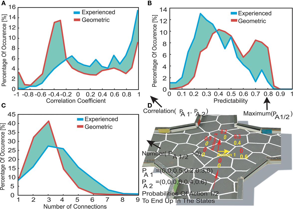
Figure 5. (A) Occurrence of correlation coefficients of the different actions. In order to do so we correlated the transition probabilities to the neighboring states of the actions as shown in the example. (B) The occurrence of the action’s highest transition probability, defined as the actions predictability. (C) The actions connectivity, defined by the number of non-zero transition probabilities for each action and state. (D) An exemplary calculation of the correlation coefficients (in A), actions predictability (in B) and the number of non-zero transition probabilities (in C), based on the transition probabilities of 2 possible actions.
Next we investigated the influence of the topographical distribution of states on the robot’s learned state transitions. Because the topographical properties of the states we used are fully represented by the geometrical transition matrix (see Materials and Methods), we took each state and action and calculated the correlation coefficient between the transition probabilities stored in the geometrical matrix and those stored in the robot’s experienced matrix. Across all actions and states, a mean correlation coefficient of 0.56 (±0.52) was obtained. Although these correlation coefficients were low, they should be considered as a conservative estimate of the similarity of action outcomes. This is because the calculation of these coefficients was based only on the transition probabilities to directly neighboring states. However, the transition probabilities to more distant states were mostly zero for all actions, and if these transition probabilities were also included in the correlation calculation, the similarity of different action outcomes would increase. In summary, while the different actions executed by the robot resulted in similar transitions more often than expected when only the topographical properties of the states were taken into account, the topographical state distribution nevertheless had an influence on the robot’s learned transitions.
How many different states can possibly be reached by means of a single action? To answer this question we examined the connectivity of the actions, by counting the number of non-zero transition probabilities. Figure 5
C shows the occurrence of this connectivity in the geometric and experienced transition matrices. The experienced transition matrix was characterized by a higher connectivity, with more than half (51%) of all actions showing a connectivity larger than four in the experienced case compared to less than a fifth (19%) in the geometric case. In the experienced case the mean connectivity was higher (3.60) than in the geometrical case (2.75). The higher connectivity in the experienced case was due to the obstacle avoidance behavior – in 79% of the experienced actions which led to more than four connected states, the robot had to use the obstacle avoidance behavior at least once. More states can be reached by executing a single action in the experienced case.
We then analyzed the predictability of action outcomes. Predictability defines the ability to predict the state that will be reached by a given action execution, and is thus useful for action planning to perceive a certain sensory outcome. In order to evaluate the actions’ predictability we introduced predictability values (see Materials and Methods) proportional to the maximum transition probability of an action. Although there are alternative ways of measuring predictability (e.g. as the sparseness of transition probabilities), these are similar to the measure used here, because of the normalization of transition probabilities to one. Figure 5
B shows the occurrence of predictability values for the experienced and geometric transition matrices. Lower predictability values (<0.3) of the actions occurred more often in the experienced case (37%) compared to the geometric one (13%). Thus in general, the robot’s actions were equally likely to reach a number of spatially adjacent states. This was due to the actions’ transition probabilities being characterized by a non-sparse probability distribution. Furthermore we investigated the influence of the obstacle avoidance behavior on the action predictability of the experienced transition matrix. Most (84%) of the low predictability values were due to actions for which the robot had to use its obstacle avoidance at least once. In other words, obstacle avoidance reduced the predictability of the action result. In most cases we obtained a lower predictability of the robot’s resultant state than we would have expected from the topographical distribution of place fields.
Impact of reflexive behavior on transition probabilities
Next we investigated the influence of the obstacle avoidance behavior on the robot’s learned transitions. The above investigations of the robot’s transitions revealed a reduction in the predictability of the robot’s actions, and an increase in the similarity between the robot’s action outcomes when compared to the transitions based on the topographical state distribution. These effects on the transitions were due to the robot’s engagement of the reflexive obstacle avoidance during these transitions. In other words, the obstacle avoidance behavior acted upon the robot’s experience-gathering behavior, thwarting the actions the robot intended to do. Here we investigated the characteristics of the transitions influenced by the reflexive behavior. The obstacle avoidance behavior was guided by proximity sensors, whose activation was highly dependent on the angle of the sensors to an obstacle. These angles can change between different trials, resulting in different sensor activations and thus in different movements of the robot. Thus the outcome of the actions combined with obstacle avoidance had a low reproducibility. A direct result of this low reproducibility was that the transition probability associated with this action would be low, given a high number of experiences. In contrast, a low number of experiences could mean that the transition probabilities of these interrupted actions was high, and would thus have a high influence on the navigational behavior. In order to analyze these effects on the transition probabilities we introduced the notion of a bad connection, defined as a low correlation between the robot’s intended actions and the transition that was learned, namely the action’s outcome. In order to quantify this relation we calculated the line between the points within a certain state at which the robot chose an action to the point within another state, at which the subsequent action was chosen. This line was compared with the direction of the action the robot intended to take. The executed action was defined as a bad connection if the angle between the line representing the robot’s traversed path and the direction of the intended action exceeded 135°. We chose this threshold because the actions with this difference in orientation had a mean correlation of 0.19 (±0.51). Figure 6
A shows the mean transition probabilities of these bad connections in the experienced transition matrix as a function of the overall number of gathered experiences. At a low amount (some hundred) of exploration steps, the average transition probability for these transitions was 0.69. With increasing exploration time, these average probabilities decayed to 0.16. The analyzed connections amounted to 29% of all connections associated with obstacle avoidance behavior. Thus, the influence on the transition matrix of obstacle avoidance resulting in a low correlation between intended and executed action reduced with an increasing number of experiences.
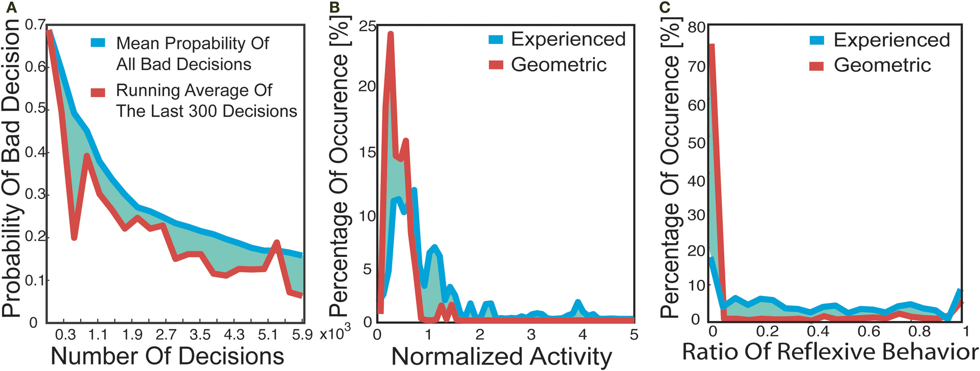
Figure 6. (A) Mean contribution to the transition probabilities of the bad decisions. Bad decision is defined as a low correlation between actions outcome and the direction of the intended action. (B) Occurrence of normalized activity in the decision-making process. (C) Ratio of executed actions which resulted in reflexive behavior.
Impact of the limited experiences
Were the differences between the geometrical properties and those learned by the robot due to the robot’s limited experience time? As outlined in the Section “Materials and Methods”, the geometrical transition matrix was generated by simulating the execution of each action on each position within a state. In order for the real-world robot to learn its environment to this extent simply by executing actions at random, it would have to experience the environment for an infinite time. In contrast, the robot’s experienced transition matrix is based on executing each action on each state 11.54 times on average (executing actions on 1.8% over all possible positions within a state; 97% overall action execution was executed only once on a position). Here we investigated the influence of this limited experience on the robot’s reduction in action predictability and the increase in the similarity between the outcomes of different executed actions. To do so, we compared the action predictability and action similarity of generated geometrical transition matrices to the geometrical transition matrix. The generated geometrical transition matrices were calculated in the same way as the geometrical transition matrix; however, the number of actions executed on each state was restricted to that of the real-world robot. We simulated 300 generated transition matrices. In order to investigate the influence of finite experience on action predictability, we calculated the action predictability values for each action of the 300 generated transition matrices. We correlated each of these 300 distributions of predictability values with that of the geometrical transition matrix and found a mean correlation of 0.89 (±0.02). In contrast, we obtained a lower similarity (r = 0.48) between the distribution of the predictability values of the robot’s experienced transition matrix and the geometrical transition matrix. The same approach was used to correlate the distributions of action similarity values of the generated transition matrices with that of the geometric transition matrix, yielding a high mean correlation of 0.93 (±0.02). In contrast, a low correlation coefficient (0.42) was found between the experienced and geometrical transition matrices. Thus, restricting the amount of experience to that of the robot had a minor effect on the generated geometric transition matrices. Finally, to directly compare the geometrical and generated transition matrices we correlated the transition probabilities for each action and state of the generated matrices with the geometric one. Averaging these correlation coefficients for each generated transition matrix yielded a distribution with a mean value of 0.86 (±0.01). A lower mean correlation coefficient (0.56) was obtained for the same correlation between the robot’s experienced and the geometric transition matrix. The difference between the transition matrix constructed from the robot’s experience and the geometrical transition matrix was thus dominated by the behavior of the robot and was not due to limited knowledge of its world.
Summary
Here we investigated the properties of the transition probabilities learned by the robot. In comparison to the transition probabilities given by the topographical distribution of states, we obtained in general a lower predictability of the outcome of the robot’s actions, as well as a higher similarity between the outcomes of different actions. These effects were mainly due to the real-world robot’s obstacle avoidance. However, despite the differences observed between the geometrical and experienced transition matrix, an influence of the topography of states on the robot’s experiences was nonetheless observed. These properties of the transitions were due to the robot’s behavior and not to the time-limited experience of the environment. Another influence of the obstacle avoidance behavior on the learned properties of the environment was given by the low correlation between the intended action and the executed action. This influence decreases as the robot increases its experience of the environment. Neglecting the reflex factors (obstacle avoidance behavior) occurring during the decision-making process, which navigational behavior would result by taking only the learned transitions into account? We would expect that it was not important for the robot to choose a precise action when moving towards a goal, due to the low action predictability as well as the high similarity between the transition probabilities of different actions. Nevertheless, the transition matrix was influenced by the geometrical distribution of the place fields, while the obstacle avoidance behavior caused a similarity between the actions and a low predictability of an action’s resultant state.
Decision-Making Process
The decision-making process involved the selection of actions in order to move to a goal, and integrates the centrally learned properties – namely the transition probabilities – and the distal learned properties – namely the reflex factors. Here we investigated the impact of distal processing on the agent’s decision-making process: first in terms of the frequency of obstacle avoidance behavior engaged in by the robot; and second by investigating the influence of the reflex values on the decision-making process. The frequency of obstacle avoidance behavior was quantified as the ratio of transitions combined with reflexive events to the total number of transitions. Figure 6
C shows the percentages of occurrence of these reflex values for the geometric and experienced case. Higher values of these ratios occurred more often in the experienced case, with a mean value of 0.42, than in the geometrical case, reflected by a mean of 0.17. This difference in means was caused by operational differences between the robot and the simulation, such as the spatial extension of the robot (see Materials and Methods), which meant that the robot-based agent used the obstacle avoidance behavior more frequently.
Next we investigated the impact of the reflex factors on the decision-making process by analyzing the normalized activity. After flooding (see Materials and Methods), the normalized activity of a state is defined as the ratio of the maximum action activation to the sum of all actions’ activations. During the decision-making process, the agent selected the action most highly activated at the robot’s current location, which meant that a low normalized activity describes a situation where all actions would result in a similar navigational performance. In contrast, high values define a decision-making process in which the agent chose a precise action in order to move to the goal. In general, this normalized activity was higher for the experienced than for the geometric transition matrix (Figure 6
B). This implies that the robot chose a precise action in order to move to a goal, and underwent a stable decision-making process. However, as discussed above, we actually expected a lower normalized activity considering only the transition probabilities. In contrast the lower reflex factors in the experienced case were due to an increase of normalized activities for the experienced transition matrix. Thus taking the reflexes into account reduced the effects of the obstacle avoidance behavior on the decision-making process, and resulted in a more precise action selection.
How did the different components of the algorithm influence the behavior of the robot? Taking only the central processes, namely the state transitions, for the decision-making into account, different action executions would result in similar navigational performances; although navigation in the narrow arms required precise actions in order to reduce wall collisions and thus reduced the path length to the goal. Integrating the distal learned environmental properties, namely reflexes, into the decision-making process, the robot now executed one precise action to navigate towards the goal. Thus as we expected, taking the distal processing into account reduces the effects of reflexive behavior and allowed the robot to successfully navigate in the environment. As mentioned above, another influence of the reflexive behavior on the transition matrix was a low correlation between intended and executed actions. This influence depended on the extent of the robot’s experience in the environment. Taking the reflexes into account reduced the number of experiences needed to neglect this effect on the navigational behavior, as the probabilities combined with obstacle avoidance behavior were reduced by the reflex factor. Thus the precise selection of an action in the decision-making process and the reduction of the number of experiences needed to navigate in the environment were due to the differentiation between a distal processing represented by the reflex values, and the central processing represented by the transition probabilities between the states, which were both integrated in the decision-making process. Differentiating between reflexive and central processing allowed the robot to successfully navigate in the environment.
Learning Behavior
Next we analyzed the plasticity of the navigation system by examining the adaptation of the robot’s navigational behavior to changes in the environment. In order to do so we inserted an obstacle into the previously learned four-arm-maze environment, as shown in Figure 7
A. We implemented and compared two different approaches to allow the robot to adapt to this change: batch and online learning (see Materials and Methods).
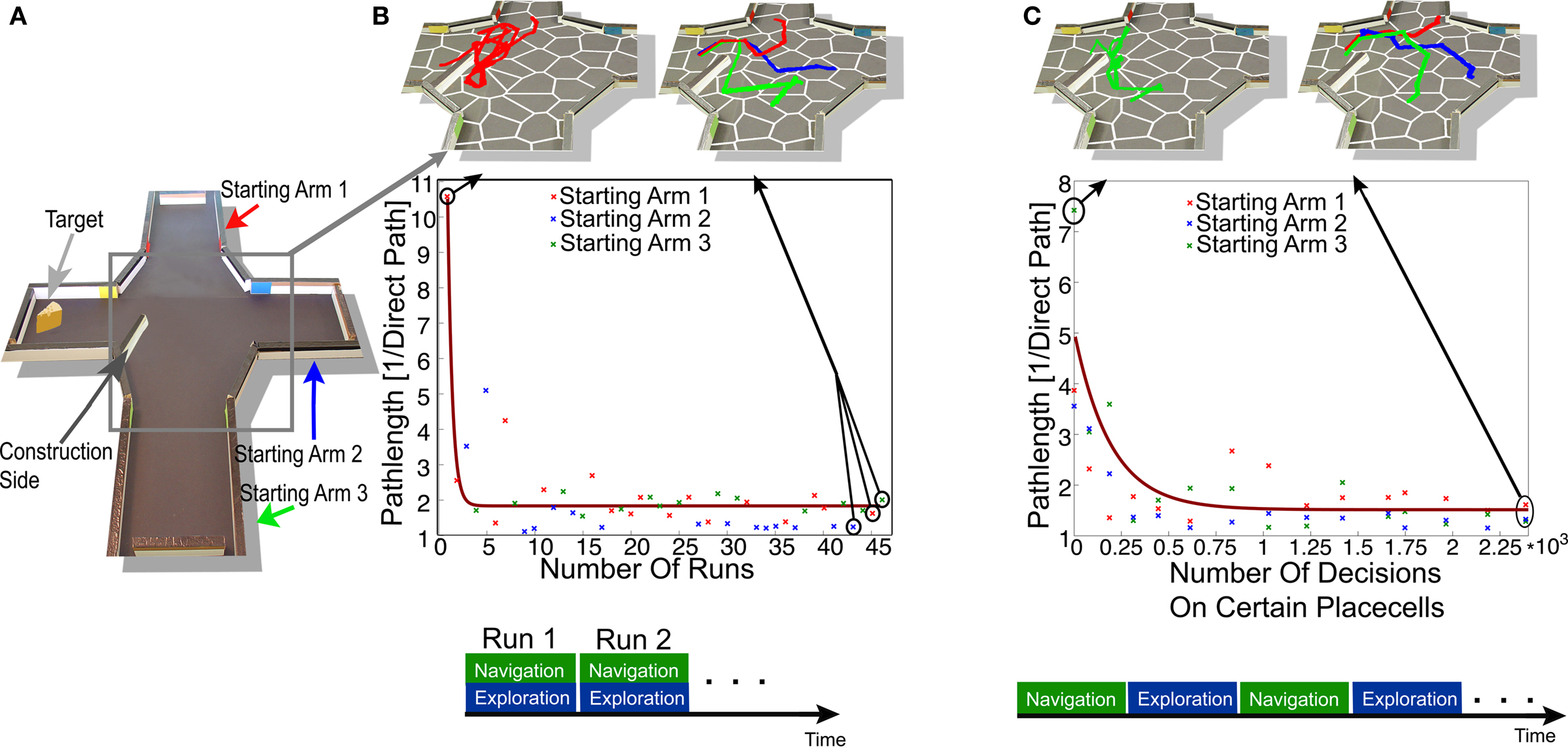
Figure 7. (A) A new obstacle (construction side) is added in an already learned environment. To test the adaptation process we evaluated the robots path through the construction side to the target side starting from three different start states, each located in one of the three different arms. (B) The adaptation process was done with online learning. This type of learning corresponds to an Exploration and Navigation stage at the same time, as shown in the lower part of the figure. The pictures in the upper part show the robot’s path in an area around the added obstacle, while the robot navigated to the target. The robot’s path length in this area is plotted in the center of this figure. The different colors correspond to the robot’s start position in the different arms as shown in (A). The brown line corresponds to the best approximation of the path length of all runs by an exponential combined with a constant. (C) The adaptation process using batch learning. After some action executions done in one of the 22 states surrounding the construction side the path of the robot from three different start states to one target side was evaluated. The robots path is shown in the upper part of the figure, for different number of experiences. In the lower part the best decision in order to move to the goal is shown for each state for a different number of experiences.
Online learning
First we investigated the adaptation process with the help of online learning by analyzing the robot’s path passing the added obstacle. In each trial the robot navigated from one start state within one of the three arms to a target site, as shown in Figure 7
A. In order to evaluate these trials we calculated the robot’s normalized path in a certain area surrounding the wall shown in Figure 7
A. Here the normalized path was given by the robot’s path in a certain area surrounding the wall, normalized by the direct path, which was the shortest traversable path between the robot’s entry and exit point of this area. The lengths of the robot’s paths are shown in Figure 7
B as a function of trial number. After a few trials (8) the path length of the robot reached values comparable to the navigational performance reported earlier. After 20 trials the selection of actions during decision-making on the different states is stabilized, and thus the changed environmental properties are fully integrated. The variation of the path length in later trials is due to the different start positions of the robot within the different arms (see Figure 7
B). Thus, online learning enabled the agent to quickly adapt to environmental changes.
As already mentioned, the navigational behavior of the system was based on two different environmental properties, stored as transition probabilities and reflexes. In order to analyze their contributions to the environmental adaptation, we compared the decision-making process based on transition probabilities and reflexes to that utilizing the transition probabilities alone. Thus we ran the flooding algorithm (as described in the Section Materials and Methods) first using the transition matrix and reflexes, and second utilizing only the transition matrix. In order to analyze the integration of the changed environmental properties into the transition matrix, we compared the action selection based only on the transition matrix before learning and after all trials of online learning. As seen in Figure 8
A, we found no difference but on two states between the best action of each state, selected only on the basis of the transition matrix, before (blue arrows) and after online learning (red arrows). Thus experience with the added obstacle was not fully integrated into the transition probabilities. In contrast, the action selection process based on both the transition matrix and the reflexes (yellow arrows) did show integration of the new environmental features. Thus, during online learning, the reflexes were responsible for the integration of the new obstacle into the decision-making process.
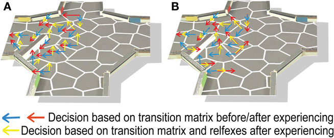
Figure 8. The best decision in order to move to the target side. The different colored arrows correspond to the different conditions. Before the robot experiences the changed environment we executed the decision-making process based only on the transition matrix without the reflex factors (Blue arrow). After the adaptation process (online learning: 45 runs/batch learning: 2500 decisions see Figure 7
) the decision process was calculated also without reflex factors based on the transition matrix (red arrow). The yellow arrows correspond to the condition of the integrated changes of the environment combined with the transition matrix and the reflexes. (A) represents the online learning while (B) batch learning.
We further investigated this integration of the changed environmental properties into the reflexes rather than the transition probabilities. The adaptation processes of the transition matrix and reflexes were dependent on the amount of actions already executed before the environment was changed (see Materials and Methods). As shown previously, without taking the reflexes into account, actions shared a similar activation value after the flooding process. In order for the transition matrix to adapt to environmental changes, the connectivity among neighboring states must change. However, we know that connected states share a similar activation due to the similarity and low predictability of the respective action outcomes, which means that any change in transition probability must be reasonably large in order to allow another action to be selected during the decision-making process. Before we added the obstacle to the four-arm-maze, the robot had experienced its environment by executing each action on each state 11.54 times on average. Thus, the robot would had to experience the changed environment for a long time before the change in transition probabilities could trigger an alternative action selection during the decision-making process. In contrast, the reflexive processing acted as a penalty on the action’s activation. Thus, the influence of the transition probabilities on the decision-making process depended directly on the activation of the neighboring states. In contrast to the influence of the reflex factors, which depended on the sum of the incoming activation for each action and thus conveniently required fewer experiences to integrate any environmental changes. As soon as the reflexes adapted to the changes in the environment, the action which led to a reflexive behavior was no longer executed during the online learning process. As a result, the adaptation process stopped. In summary, during online learning it is the reflexive processing that enabled a fast integration of the environmental changes.
Batch learning
Next we investigated the adaptation process involved in batch learning and compared it to online learning. Each of the experience stages was specified by the number of action execution done on each of the 22 states surrounding the added obstacle. In order to evaluate the robots navigational performance, the robot navigated in each navigation stage two times from three different start positions within one arm to the target site. The average normalized path within a certain area around the added obstacle, for each start position is shown in Figure 7
C. After an experience stage containing around 500 experiences, the path length of the robot reached a length comparable to the robot’s best navigational performance reported earlier. A slight increase in the path length can be seen after 800 experiences. This was due to some new learned features of the environment. As the obstacle was located in the middle of a state, actions were executed which results in a reflexive behavior on one side of the obstacle and on the other side not. Thus in this case batch learning could result in some instability in the decision-making process, according to some conflicting experiences learned in the environment. After 1500 randomly executed actions the navigational performance did not change much anymore and in general the best actions in order move to the target did not change anymore. Thus after a short amount of time the changed environmental features were integrated in the navigational performance by batch learning. Here, the robot needed more time to experience the environment compared to online learning. This was due to the difference types of learning, as online learning integrated only the environmental features in order to move to the goal while batch learning was latent learning and thus could integrate any changed features. However after a short amount of time online and batch learning integrated the environmental changes in their navigational behavior.
Also here we analyzed the contribution of the transition probabilities and the reflex factors to the navigational adaptation. As done for online learning we analyzed the decision-making process by comparison of the decision-making process based on the transition matrix and reflexes with the one based on only the transition matrix. We concluded from Figure 8
B that also the transition probabilities adapted to the changes in the environment. Thus in contrast to online learning, during batch learning the transition probabilities were able to integrate the changed environmental features.
Differentiating between reflexive and central processing allowed the robot to successfully navigate in the environment. This differentiation also resulted in a fast integration of the environmental changes and thus navigational adaptation to the changes in the environment. The presented architecture was able to successfully model navigational behavior and kept its plasticity in an already learned environment.
We have introduced a cognitive model capable of generalizing over a broad variety of behavioral domains, and applied it to a navigational task. Here, behavior was modeled as state transitions in the state space spanned by place cells. Furthermore, the architecture of this model differentiated between central processing and distal processing. Distal processing was defined by the state transitions where the reflexive behavior of the sensory-driven obstacle avoidance was triggered. Central processing acted on all learned transitions between states. The reflexive behavior acted upon the robot’s learned transitions, resulting in uniformly distributed and less predictable action outcomes than expected from inspection of the topographical distribution of place fields used. However, as expected, the integration of the information gained by reflexive and central processing in the decision-making process reduced the impact of sensory-driven obstacle avoidance behavior on the navigational performance. In addition the introduced model quickly adapted to changes in the environment. Consequently, the robot was able to successfully navigate in the real-world environment after only a short amount of time.
Here we used eight different discrete actions in order to limit the robot’s experience time. The outcome of these different actions resulted in redundancies, which would increase by increasing the number of actions. Consequently the robot would not gain more information about the environment by more action possibilities. In addition using discrete actions allows the cognitive architecture to be easily expandable. Without a change of concepts it might be applied to a robot equipped with a grabber to lift object. In order to capture such a behavior the state space has to be expanded, such that each sensory state is defined by a spatial state (place fields) and the position of an object, either at the bottom or at the top lifted by the grabber. This state space representation could not be embedded in a 2D space, but necessitates a high-dimensional representation. However, learning transition probabilities and reflex factors does not refer to the dimensionality of state space and the same algorithms might be applied. The agent has to experience the transition probabilities of this new sensory state space by executing its action, consisting of the movement of the grabber and the eight different directions. In order to let the robot lift an object the corresponding sensory state has to be activated an this activity has to be back propagated as described in the Section Materials and Methods. Thus the discretization of the action makes it easy to apply the cognitive model to different behaviors and expand the action repertoire with different unrelated actions, like lifting objects. Admittedly, in a very high-dimensional state space new problems due to very sparse data arise. This, however, is a general problem of large non-hierarchical state spaces and beyond the scope of the present work. In this cognitive architecture the limitation on modeling different behaviors is given by the robot’s experience time, which increases with the number of states and actions and thus with the complexity of the behavior to be modeled.
The decision-making process involves two parameters, the decay factor and a parameter in the reflex value (see Decision making). The decay factor is also known as discounting factor (Sutton and Barto, 1998
) and was introduced to reduce the number of transitions needed to move to the goal. In case of a small decay factor, the agent preferred to make fewer transitions to move to the goal and thus make also those transitions characterized by low predictability, i.e. low reliability. In order to reduce unreliable transitions and thus the variation of pathlength to the goal between different runs, we chose a decay value of 0.9, used in most literature (Sutton and Barto, 1998
). However a change of the decay value between 0.6 and 0.95 did not affect the decision-making process much. Further, to calculate the reflex values we weighted the ratio of transitions associated with a reflexive event to all over transitions with a factor of 5/6. In case of a weighting factor smaller than 5/6 the reflexive events would be less involved in the decision-making process, such that the agent prevents less transition associated with a reflexive event in order to move to the goal. An increase of the weighting factor would result in an opposite behavior, while at a value of one transitions would be not considered in the decision-making process in case all transitions are associated with an reflexive event, which are obtained at the narrow arms. Thus, such a weighting factor would reduce the agent’s navigability especially at the narrow arms. However, a change of the weighting factors between 0.5 and 0.95 does not have a huge impact on the decision-making process. Thus, in a certain range the variation of the parameters have a small impact on the agent’s navigational behavior.
Further we characterized the computational complexity of the reverse flooding procedure. In each iteration the activity of each state is propagated to all other states as defined by the transition probabilities (see Action Execution). This implies a multiplication of the transition matrix with the state vector, resulting in O(N2) operations for N states. However, as the transition matrix is highly sparse, the effective number non-zero transition probabilities is much lower. Specifically, scaling behavior depends on the number of connected states as a function of total number of states. In the context of the present study, increasing the size of the arena at constant spatial resolution lead to a linear scaling.
Complementary to the cost of each iteration, the number of iterations was estimated. In the present implementation the number of iterations is determined by a threshold criteria. When the sum of absolute changes of state activation was smaller than 10−5 the flooding procedure was terminated (Figure 2
). Due to the sparseness of the transition matrix the interaction of two states needs a finite number of iterations, in the worst case limited by N, i.e. the process is O(N). In the typical scenario, however, the reverse flooding reaches the target state much faster on the scale of the length of the final trajectory. During this activity propagation the decay factor affects the activity such that it exponentially decays with the number of iterations (Figure 2
). This punishes long trajectories, and for practical purposes, the winning trajectory was always of a length comparable to the one leading to the fastest interaction. In the context of the present experiments this leads to a scaling of O(N1/2). A strict upper bound is dependent on the topology of the problem. Specifically, the sparser the transition matrix is, the cheaper a single iteration can be computed, but the number of necessary iterations increases. For a non-sparse transition matrix a single iteration is more expensive, but the number of necessary iterations is reduced. As an estimate of the computational expense of the total computational costs of the algorithm presented above we obtain a scaling of better than O(N3). This is not cheap, but clearly computationally tractable.
Next we discuss the computational complexity involved in the application of the cognitive architecture in a context other than navigation. Under natural conditions simple cells in primary visual cortex display sparse activity. Indeed, recent studies propose that sensory representations of natural stimuli optimize specific statistical properties like sparseness (Olshausen and Field, 1996
), temporal coherence (Körding et al., 2004
; Wyss et al., 2006
) and predictability (König and Krüger, 2006
; Sprekeler et al., 2007
). In line with this research, we suggest that sensory states in general are optimal for predicting the action induced state transitions (Weiller et al., submitted). This implies that the transition matrix of such highly predictable sensory representations contain either rather high or low and few mid-level probabilities, i.e. they are sparse. This property, as argued above, leads to benign scaling behavior. We like to point out that this is not a worst-case analysis. To the contrary, it is based on the assumption that the properties of sensory representations are optimized with respect to the available behavioral repertoire. Hence we hypothesize, that the presented cognitive architecture has tractable computational complexity exactly for the relevant scenarios, but not necessarily in general.
Different studies have modeled navigational behavior by using place cells as a representation of the environment. These different approaches can be characterized by the type of learning used: Hebbian learning or reinforcement learning. The first type of learning exploits the fact that while moving in the environment, more than one place cell is active at the rodent’s location, caused by the overlapping place fields of the corresponding cells. This allows the application of the biologically motivated principles of LTP and LTD, resulting in a strengthening of the connections between place cells which were active in a certain time interval. These cells and their connections between each other represent a cognitive map (Blum and Abbott, 1996
; Gerstner and Abott, 1997
; Gaussier et al., 2002
). Other studies introduced a cell type – goal cells – representing the goal of the navigational task (Burgess et al., 1997
; Trullier and Meyer, 2000
). The connections between the current place and the goal cell encode the place cell’s direction to the goal. The strength of connections between these two cell types was also modulated by Hebbian learning. In contrast to our model, the mentioned approaches rely on a global orientation and a metric, measuring the direction and distance to the goal from a given location within the environment. The global orientation used by these studies is defined using the same frame of reference over the whole environment. In contrast, we wanted the robot to learn the topology of the environment and thus did not introduce such global variables as orientation or a metric. Furthermore, some of the mentioned studies (Burgess et al., 1997
; Gerstner and Abbott, 1997
; Foster et al., 2000
; Trullier and Meyer, 2000
; Strosslin et al., 2005
) used population coding to encode the position or direction to the goal. The population vector approach is based on the assumption that place fields and rodent’s orientations have separate topologies. Thus to decode the robot’s position or orientation, the weighted average of place cells or orientations has to be calculated. This incorporates knowledge of the topology in the decoding scheme and impedes a generalization to other action repertoires. In contrast, we defined the actions independently of each other so that the action repertoire can easily be expanded, for example including the action of lifting an object. Cuperlier et al. (2007)
suggested a navigation algorithm based on learned transitions between activity patterns of place cells. In this study only connections between place cells with their neighbors were allowed, predefining a topology to be learned. Further, in the mentioned work the agent’s location within the environment is associated with an activity pattern of place cells. In contrast we defined a state space by applying a winner take all process on the place cells activity. We can hypothesize that the transitions captured by Cuperlier and colleagues are not as sparse as the one used here. This is due to the possibility to establish transitions from place cells with an activity value smaller than the maximum activity and larger than zero. Other branches of studies (Arleo and Gerstner, 2000
; Foster et al., 2000
; Arleo et al., 2004
; Strosslin et al., 2005
) used reinforcement learning (Sutton and Barto, 1998
) to perform a navigational task. The concepts of Markov Decision Processes and value iteration (Sutton and Barto, 1998
) are commonalities between reinforcement learning and our approach, while in our model, value iteration was expanded by reflexes. A pure reinforcement learning approach involves learning the properties of the environment by using an explicit reinforcement signal, given by a goal state; in the presented model these properties are latently learned (Tolman, 1948
), resulting in a global strategy for navigation in this environment. In contrast to other studies, here we have presented a cognitive model that is able to learn the topology and properties of the environment in a latent manner and can additionally be expanded to model other behaviors by redefining the meaning of the actions and states.
In the introduced cognitive model we differentiated between central and distal processing, the latter driven by the reactive obstacle avoidance behavior. In order to control autonomous robots, one approach tries to utilizes reactive controller, which selects the next action as a function of the current sensor readings. Millan’s (1996)
approach tries to combine traditional reinforcement learning with reactive learning procedure. Thus traditionally reinforcement learning in a navigational paradigm evaluates the quality of an action to reach a global goal. In this work a negative reinforcement is given when the robot facilitates its collision sensors to do obstacle avoidance. While in the mentioned study, environmental properties are learned for a particular goal, here we learned the environmental properties in a latent way, such that we are able navigate to different goals in the environment. Similar to Millan our cognitive agent can easily adapt to changes of the environment. In summary, by learning the environmental properties in a latent way, the robot is able to navigate to different goals in the environment, while differentiating between central and distal components results in a fast adaptation to changes of the environment.
The introduced cognitive model is based on a sensory representation composed of discrete states. In this state space the robot first learned the sensory outcomes of its action’s execution, namely the state transition and the reflex factors. Thus, the robot learned the environmental properties in an unsupervised fashion with respect to its actions. Based on these results, the robot planned its action in order to move to the goal state. We defined the states such that they are equivalent to the place fields of place cells, providing a representation of body position within the external space. Although the contribution of place cells to the rodent’s navigational performance is not fully understood, an involvement of these cells has been obtained (Morris et al., 1982
). These place cells can be understood as an optimally stable sensory representation of the visual input to a robot moving in an environment (Wyss et al., 2006
). The unsupervised learning resulted in a reorganization of the sensory space spanned by the robot’s visual input, leading to a low-dimensional representation of the sensory input with a spatial interpretation. In order to determine the robot’s current state, we used a winner takes-all process over all place cells’ current activations. This process results in a discrete division of the robot’s navigational space, spanned by the robot’s possible positions. Since this navigational space completely determines the navigational task, a discrete division of this space corresponds to a discrete division of any sensory space relevant for navigation (e.g. the sensory space spanned by the proximity sensors, which measure distances to objects). In this study we used predefined place cells and used a tracking camera to determine the place cells activities. This complements a previous study on unsupervised learning, using a frontal camera of the robot, to form place cells at high levels of the sensory hierarchy (Wyss et al., 2006
). In ongoing work we combine these two approaches to generate appropriate behavior in an autonomous agent based on local sensory only. In addition, differentiating between distal processes – namely the transitions influenced by the sensory-driven behavior – and central processes – the state transitions – is expected to result in a better performance of the system. In order to extend our model to different behaviors, we need only to divide the relevant sensory space into discrete states and implement the actions that define the behavior to be modeled. By means of executing these actions, the sensory outcome in the state space can be learned.
The number of actions influences the agent’s navigational performance. Given a state space, increasing the number of action possibilities, i.e. the behavioral repertoire, allows more appropriate actions and is expected to lead to a small improvement of navigational performance. Such an expansion of the behavioral repertoire does not change the principles of the presented model, but only increases the number of learned transitions, scaling linear with the number of actions. However, increasing the action possibilities above a certain number would result in a high similarity between the actions transition probabilities and thus does not result in an increase of the navigational performance. Hence, the discretization of the action space should be in a reasonable relation to noise level of actions, defined in this study by the robot’s angular precision.
Also the number of discrete states influences the navigational performance. Increasing the number of states would not only increase the navigational performance but also the precision of spatial navigation. An increase of the number of states allows the agent to capture the navigational properties of the environment more precisely in its transition probabilities. This would result in a better navigational performance of the agent. Further, increasing the number of states allows the agent to navigate to a more precise position within the environment. But increasing the states results raises the time needed to experience the environment, which scales linearly with the number of states. Here, we chose a state representation, which is balanced between navigability and representational parsimony, and thus restricted the agent’s time to explore the environment.
We have introduced a cognitive architecture for the modeling of animal-like behavior, and plan to use this model to obtain further insights into the general principles of behavior, such as action planning. The model is based on a discrete division of sensory space into states, and here the state space was obtained by randomly distributing place cells in the environment. The topographical distribution of these states was shown to influence the transition probabilities, and thus to affect the robot’s behavior. This raises the important question of how these states should be organized to allow the robot to behave optimally. In other words, how can we optimally reorganize the sensory space, given only the sensory input and the robot’s action repertoire? This corresponds to a reorganization of the somatosensory space, which is recently highly discussed topic (Moore, 1991
; McCallum, 1993
; Singh et al., 1995
; Kaplan and Oudeyer, 2007
; Oudeyer et al., 2007
). As our model can generalize over different behavioral domains, we claim that it can be employed to gain insights into different behavioral principles such as those mentioned here.
The authors declare that the research was conducted in the absence of any commercial or financial relationships that could be construed as a potential conflict of interest.