Bayesian state estimation in partially-observed dynamic multidisciplinary systems

1 Introduction

The world, shaped as it is today by the progress in science and technology, is marked by the development of new, increasingly complex engineering systems. These systems often consist of several disciplines interacting with each other, typically with a great deal of uncertainty associated with each discipline (Ghoreishi, 2016). In these complicated multidisciplinary systems, the interaction between disciplines can be feedforward coupling (in which case, the output of an upstream discipline becomes an input to a downstream discipline) or the interaction can be feedback coupling (in such a way that the output of one discipline is input to the other discipline and vice versa). Coupled multidisciplinary systems are found in many applications, particularly in aerospace engineering, such as modeling aerostructural-thermal coupling in hypersonic flight (Culler and McNamara, 2010), turbine-engine cycle analysis (Hearn et al., 2016), satellite performance analysis (Larson and Wertz, 1992; Zaman and Mahadevan, 2013), topology optimization (Dunning et al., 2011), and more.

Analysis and optimization of multidisciplinary systems have been extensive areas of research, and numerous studies in the literature have dealt with various aspects of multidisciplinary analysis in several engineering disciplines (Sobieszczanski-Sobieski and Haftka, 1997; Hart and Vlahopoulos, 2010; Yao et al., 2011; Meng et al., 2015; Zhang et al., 2016a; Zhang et al., 2016b; Friedman et al., 2018). Researchers have focused on the development of computational methods (Cramer et al., 1994; Agarwal et al., 2004; Ghoreishi and Allaire, 2017) and the application of these methods for multidisciplinary systems design, analysis, and optimization (Agarwal and Renaud, 2004; Guo and Du, 2010; Ghoreishi and Imani, 2020). Many researchers have studied the reliability analysis and uncertainty propagation in the design of coupled multidisciplinary systems (Gu et al., 2000; Du and Chen, 2005; Du et al., 2008; Ghoreishi and Allaire, 2016; Friedman et al., 2017; Ghoreishi and Imani, 2021).

Despite the broad research on the analysis of multidisciplinary systems and the wide spectrum of developed techniques in this area, most of the aforementioned studies have focused on the stationary analysis of systems without taking their dynamic behavior into account. However, the transient interactions between the disciplines can put the system at risk if the temporal evolution of the system is not accounted for in the design, control, and reliability analysis of multidisciplinary systems. Moreover, the disciplines are often partially observed as they are monitored through noisy sensor measurements. Therefore, for the robust analysis of multidisciplinary systems for the purpose of design or control, there is a need to study their dynamic behavior under partial information obtained through noisy sensors.

The goal of this paper is the dynamic analysis of coupled multidisciplinary systems from imperfect information acquired from noisy sensors. The real-time monitoring of these coupled multidisciplinary systems is often challenging due to the large number of disciplines and the complex interactions between the disciplines. Reliable monitoring and analysis of these complex systems demand for an accurate estimation of the system’s state over time. Toward this, we present a general nonlinear/non-Gaussian state-space representation of coupled multidisciplinary systems. Using the proposed probabilistic state-space formulation, we derive a particle filtering approach for dynamic state estimation of multidisciplinary systems in the presence of noisy measurements. The proposed framework enables the precise estimation of the system state over time for effective control, design, and analysis of coupled multidisciplinary systems.

The article is organized as follows. In Section 2, the detailed description of the proposed state-space model for coupled multidisciplinary systems is provided, followed by the state estimation process via sequential importance resampling (SIR) particle filter in Section 3. Section 4 presents the numerical experiments demonstrating the state estimation results on a coupled aerodynamics-structures system and a coupled three-discipline fire detection satellite. Finally, Section 5 contains the concluding remarks.

2 Partially-observed dynamic multidisciplinary systems

A generic multidisciplinary system consists of a set of interconnected disciplines that interact with other. The interaction between two disciplines depends on the direction of information flow; this interaction can be feedforward (unidirectional) coupling or feedback (bidirectional) coupling. A feedback coupled multidisciplinary system with d disciplines interacting with each other dynamically at each time k can be represented as (Asadi and Ghoreishi, 2022):

${\mathbf{c}}_{ij}\left(k\right)=f_i\left({\mathbf{c}}_{ji}\left(k-1\right),{\mathbf{u}}_i\left(k-1\right)\right)+{\mathbf{v}}_i\left(k\right),(1)$

for i, j = 1, … d; i ≠ j, where c_ij(.) is the vector of coupling variables output from discipline i and input to discipline j, u_i(.) is the vector of inputs (either independent or shared between different disciplines) to discipline i other than the coupling variables, f_i(.) is the function associated with discipline i, and v_i(.) is the uncertainty accounting for unmodeled parts of discipline i.

2.1 State-space model

In multidisciplinary systems, the coupling variables are the variables that are shared among multiple disciplines, indicating the disciplines’ internal behavior, which affect other disciplines’ behavior as they get fed into other disciplines; overall, affecting the behavior of the system over time as a result of all couplings. Therefore, coupling variables are the hidden parts of the system that determine the interactions between disciplines and provide insights about the system-level behavior. In multidisciplinary systems, precisely estimating the values of coupling variables at each time is required in order to achieve effective control, design, and analysis of the system. In fact, estimating the correct state of the coupling variables allows one to have accurate knowledge about the current state of the multidisciplinary system as a whole and, consequently, to make informed decisions when choosing control or design inputs to the system or disciplines. Having the functional model of coupled multidisciplinary systems in Eq. 1, we present a general nonlinear/non-Gaussian state-space representation of coupled multidisciplinary systems. We consider ${\mathbf{x}}_k\in \mathbb{X}$ as the state vector of the system at time step k (k = 1, 2, …), containing all coupling variables of the multidisciplinary system, defined as:

${\mathbf{x}}_k=\left\{{\mathbf{c}}_{ij}\left(k\right)\mid i,j=1,\dots d;i\ne j\right\},(2)$

and ${\mathbf{u}}_k\in \mathbb{U}$ as the vector of inputs to all disciplines, excluding the coupling variables:

${\mathbf{u}}_k=\left\{{\mathbf{u}}_i\left(k\right)\mid i=1,\dots d\right\}.(3)$

We define f(.) as the vector containing all discipline functions:

$\mathbf{f}=\left\{f_i\mid i=1,\dots d\right\},(4)$

that is possibly nonlinear and time-varying, describing the evolution of the state, i.e., the state dynamics. In multidisciplinary systems, the coupling variables are often not directly observable, but some noisy and/or partial observations of the states are often available, acquired via sensors. Having these definitions, we consider the following nonlinear state-space model describing the system and measurement models as:

$\begin{array}{ccc}\hfill {\mathbf{x}}_k& =\hfill & \mathbf{f}\left({\mathbf{x}}_{k-1},{\mathbf{u}}_{k-1}\right)+{\mathbf{v}}_k\left(\text{system\hspace{0.17em}model}\right)\hfill \\ \hfill {\mathbf{z}}_k& =\hfill & \mathbf{h}\left({\mathbf{x}}_k\right)+{\mathbf{w}}_k\left(\text{measurement\hspace{0.17em}model}\right)\hfill \end{array}(5)$

where v_k is the system noise with probability distribution p_v (i.e., v_k ∼ p_v) containing the unmodeled parts of the system dynamics, ${\mathbf{z}}_k\in \mathbb{Z}$ is a vector of noisy measurements, w_k from the probability distribution of p_w (i.e., w_k ∼ p_w) represents the measurement noise due to sensor imprecisions, and h(.) is a (possibly nonlinear) function mapping the states to the measurements, for k = 1, 2, …. The system and measurement noises v_k and w_k are assumed to be white in the sense that the noises at distinct time points are independent random variables (i.e., v_k and v_l, and similarly w_k and w_l, are independent for k ≠ l). It is also assumed that the noise processes are independent from each other and from the initial state x₀; their distribution is otherwise arbitrary.

For a two-disciplinary system, assuming that the measurements are from the states in solo and a combination of both, the state-space model can be presented as:

$\underset{{\mathbf{x}}_k}{\underbrace{\left[\begin{array}{c}\hfill {\mathbf{c}}_{12}\left(k\right)\hfill \\ \hfill {\mathbf{c}}_{21}\left(k\right)\hfill \end{array}\right]}}=\underset{\mathbf{f}\left({\mathbf{x}}_{k-1},{\mathbf{u}}_{k-1}\right)}{\underbrace{\left[\begin{array}{c}\hfill f_1\left({\mathbf{c}}_{21}\left(k-1\right),{\mathbf{u}}_1\left(k-1\right)\right)\hfill \\ \hfill f_2\left({\mathbf{c}}_{12}\left(k-1\right),{\mathbf{u}}_2\left(k-1\right)\right)\hfill \end{array}\right]}}+\underset{{\mathbf{v}}_k}{\underbrace{\left[\begin{array}{c}\hfill {\mathbf{v}}_1\left(k\right)\hfill \\ \hfill {\mathbf{v}}_2\left(k\right)\hfill \end{array}\right]}},$

$\underset{{\mathbf{z}}_k}{\underbrace{\left[\begin{array}{c}\hfill {\mathbf{z}}_1\left(k\right)\hfill \\ \hfill {\mathbf{z}}_2\left(k\right)\hfill \\ \hfill {\mathbf{z}}_3\left(k\right)\hfill \end{array}\right]}}=\underset{\mathbf{h}\left({\mathbf{x}}_k\right)}{\underbrace{\left[\begin{array}{c}\hfill h_1\left({\mathbf{c}}_{12}\left(k\right)\right)\hfill \\ \hfill h_2\left({\mathbf{c}}_{21}\left(k\right)\right)\hfill \\ \hfill h_3\left({\mathbf{c}}_{12}\left(k\right),{\mathbf{c}}_{21}\left(k\right)\right)\hfill \end{array}\right]}}+\underset{{\mathbf{w}}_k}{\underbrace{\left[\begin{array}{c}\hfill {\mathbf{w}}_1\left(k\right)\hfill \\ \hfill {\mathbf{w}}_2\left(k\right)\hfill \\ \hfill {\mathbf{w}}_3\left(k\right)\hfill \end{array}\right]}}.$

Clearly, the size of the measurement vector can be different (smaller or larger) from the size of the state vector, depending on the number of sensors and type of measurements in the system.

3 State estimation in partially-observed dynamic multidisciplinary systems

The general idea of the optimal state estimation filtering problem in state-space models is to compute an optimal estimate for the true value of the system state at time k, i.e., x_k, from an incomplete, potentially noisy set of observations Z_1:k = (z₁, … , z_k) made on the system and inputs U_1:k = (u₁, … , u_k) to the system. In the Bayesian approach to dynamic state estimation, the posterior state given all measurements and inputs up to time k is constructed as:

$p\left({\mathbf{x}}_k\mid {\mathbf{Z}}_{1:k},{\mathbf{U}}_{1:k}\right).(6)$

In the remainder, the sequence of inputs will be left out for ease of notation. In many design problems and analyses of multidisciplinary systems, it is required to estimate the system state every time that a noisy measurement is received. This state estimation can be achieved by recursively applying the prediction and update stages of Bayesian filtering approaches (Arulampalam et al., 2002).

Let p(x_k−1∣Z_1:k−1) be the available conditional distribution of the state at time step k—1 given measurements Z_1:k−1. In the prediction stage of the filter, according to the Chapman–Kolmogorov equation under the Markovian property of the system model in Eq. 5, the state at time k can be predicted as:

$p\left({\mathbf{x}}_k\mid {\mathbf{Z}}_{1:k-1}\right)=\mathit{\int }p\left({\mathbf{x}}_k\mid {\mathbf{x}}_{k-1}\right)p\left({\mathbf{x}}_{k-1}\mid {\mathbf{Z}}_{1:k-1}\right)d{\mathbf{x}}_{k-1}.(7)$

In this prediction stage, the Markov process of order one in the system model in Eq. 5 that provides a probabilistic model of the state evolution, allows us to use the fact that p(x_k∣x_k−1, Z_1:k−1) = p(x_k∣x_k−1).

After observing the measurement z_k at time step k, the state estimate at time step k using the Bayes’ theorem can be updated to:

$p\left({\mathbf{x}}_k\mid {\mathbf{Z}}_{1:k}\right)=\frac{p\left({\mathbf{z}}_k,{\mathbf{x}}_k\mid {\mathbf{Z}}_{1:k-1}\right)}{p\left({\mathbf{z}}_k\mid {\mathbf{Z}}_{1:k-1}\right)}=\frac{p\left({\mathbf{z}}_k\mid {\mathbf{x}}_k\right)p\left({\mathbf{x}}_k\mid {\mathbf{Z}}_{1:k-1}\right)}{p\left({\mathbf{z}}_k\mid {\mathbf{Z}}_{1:k-1}\right)},(8)$

where the likelihood p(z_k∣x_k) representing the conditional probability of the measurement z_k given the predicted state x_k can be obtained from the measurement model in Eq. 5 and the known statistics of the measurement noise v_k, p(x_k∣Z_1:k−1) is the prior computed in Eq. 7 and the normalizing constant can be computed as:

$p\left({\mathbf{z}}_k\mid {\mathbf{Z}}_{1:k-1}\right)=\mathit{\int }p\left({\mathbf{z}}_k\mid {\mathbf{x}}_k\right)p\left({\mathbf{x}}_k\mid {\mathbf{Z}}_{1:k-1}\right)d{\mathbf{x}}_k.(9)$

The recurrence relations in Eqs 7, 8 construct the “prediction” and “update” stages of the optimal Bayesian solution that cannot be determined analytically, and particle filters or sequential Monte Carlo methods as a set of Monte Carlo (MC) algorithms can be used to solve the filtering problem approximately.

3.1 Sequential importance resampling filter

Sequential Importance Resampling (SIR) (Gordon et al., 1993) filter is a common particle filter that can be applied to recursive Bayesian state estimation. The key idea in SIR is to approximate a target posterior density function p(x) using a set of random samples ${\{{\mathbf{x}}_i\}}_{i=1}^N$ drawn from a proposal distribution q(x) that is easier to sample from. The bias created by sampling from the proposal instead of the target is compensated by associating proper weights ${\{{\mathit{\omega }}_i\}}_{i=1}^N$ to the samples, computed as:

${\mathit{\omega }}_i\propto \frac{p\left({\mathbf{x}}_i\right)}{q\left({\mathbf{x}}_i\right)},(10)$

where the associated weights are normalized such that ${\sum }_{i=1}^N{\mathit{\omega }}_i=1$. Then, a weighted approximation to the density p(.) is given by:

$p\left(\mathbf{x}\right)\approx \sum _{i=1}^N{\mathit{\omega }}_i\delta \left(\mathbf{x}-{\mathbf{x}}_i\right),(11)$

where δ(.) denotes the Dirac delta function. Importance resampling, which is based on the Radon-Nikodynm theorem (Glynn and Iglehart, 1989), allows us to draw samples from the target distribution by re-weighting the samples drawn from the proposal distribution, and then resample from them with replacement. The iterative re-weighting of available sample information to compute estimates based on these samples and weights is achieved using sequential importance resampling (SIR). SIR will consist of independent draws from p(.) as N → ∞ (Smith and Gelfand, 1992).

Returning to the recursive Bayesian state estimation problem, the target density function is the posterior density function of state at time step k given all measurements up to time k, i.e., p(x_k∣Z_1:k), that can be derived as:

$p\left({\mathbf{x}}_k\mid {\mathbf{Z}}_{1:k}\right)\propto p\left({\mathbf{z}}_k\mid {\mathbf{x}}_k\right)p\left({\mathbf{x}}_k\mid {\mathbf{x}}_{k-1}\right)p\left({\mathbf{x}}_{k-1}\mid {\mathbf{Z}}_{1:k-1}\right).(12)$

We consider p(x_k∣x_k−1) as the proposal distribution that is easy to be sampled as the system dynamics is known in Eq. 5. We start the particle-based state estimation by drawing N particles from the initial state distribution as:

${\left\{{\mathbf{x}}_{0,i}\right\}}_{i=1}^N\sim {\pi }_0,(13)$

where π₀ represents the initial belief about the distribution of states, and the associated weights are set to ${\{{\omega }_{0,i}\}}_{i=1}^N=\frac{1}{N}$. Assuming that the pairs ${\{{\mathbf{x}}_{k-1,i},{\mathit{\omega }}_{k-1,i}\}}_{i=1}^N$ consist of the particles and their associated weights at time k—1 approximating p(x_k−1∣Z_1:k−1), the particles ${\{{\mathbf{x}}_{k,i}\}}_{i=1}^N$ representing p(x_k,i∣x_k−1,i) can be obtained as:

${\mathbf{x}}_{k,i}\sim \mathbf{f}\left({\mathbf{x}}_{k-1,i},{\mathbf{u}}_k,{\mathbf{v}}_k\right),(14)$

and their associated weights at time k according to Eq. 12 can be updated as:

${\mathit{\omega }}_{k,i}\propto p\left({\mathbf{z}}_k\mid {\mathbf{x}}_{k,i}\right){\mathit{\omega }}_{k-1,i}.(15)$

However, noting that resampling is applied at every time step, we have ${\{{\mathit{\omega }}_{k-1,i}\}}_{i=1}^N=1/N$; therefore

${\mathit{\omega }}_{k,i}\propto p\left({\mathbf{z}}_k\mid {\mathbf{x}}_{k,i}\right).(16)$

The weights given by the proportionality in Eq. 16 are then normalized, which construct a categorical distribution. Categorical distribution is a discrete probability distribution describing the probability that a random variable will take on a value that belongs to one of N categories, where each category has a probability associated with it. After drawing N samples from this distribution in the resampling process, we achieve the set ${\{{\mathbf{x}}_{k,i},{\mathit{\omega }}_{k,i}\}}_{i=1}^N$. Finally, the conditional distribution of the state at time step k, can be computed as:

$p\left({\mathbf{x}}_k\mid {\mathbf{Z}}_{1:k}\right)\approx \sum _{i=1}^N{\mathit{\omega }}_{k,i}\delta \left({\mathbf{x}}_k-{\mathbf{x}}_{k,i}\right).(17)$

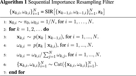
The computational complexity of SIR particle filter at each time step is O(N) (Doucet et al., 2009). An iteration of SIR is presented in Algorithm 1.

4 Numerical experiments

In this section, the SIR particle filter is implemented for state estimation of a coupled aerodynamics-structures system and a three-discipline fire detection satellite.

4.1 Coupled aerodynamics-structures system

The first problem is a two-dimensional airfoil in airflow model adapted from (Sobieszczanski-Sobieski, 1990). Figure 1 shows this system in which the airfoil is supported by two linear springs attached to a ramp and the airfoil is permitted to pitch and plunge. A complete description of the problem can be found in (Sobieszczanski-Sobieski, 1990). A block diagram of the system is shown in Figure 2. In this problem, the coupling variables are the lift L and the elastic pitch angle ϕ which are the system states represented as:

$\begin{array}{cc}\hfill L_k=& qBC\left(2\pi \left({\varphi }_{k-1}+\psi \right)+r\left[1-\cos \left(\frac{\pi }{2}\frac{\left({\varphi }_{k-1}+\psi \right)}{{\theta }_0}\right)\right]\right)+v_{L,k},\hfill \\ \hfill {\varphi }_k=& \left(\frac{L_{k-1}}{k_1\left(1+p\right)}-\frac{L_{k-1}p}{k_2\left(1+p\right)}\right)\frac{1}{C\left({\bar{z}}_2-{\bar{z}}_1\right)}+v_{\varphi ,k},\hfill \end{array}(18)$

where q = 1 N/cm², B(span) = 100, C(chord) = 10 cm, ψ = 0.05 rad, r = 0.9425, θ₀ = 0.26 rad, p = 0.1111, k₁ = 4000 N/cm, k₂ = 2000 N/cm, ${\bar{z}}_1=0.2$, and ${\bar{z}}_2=0.7$. The state noises are assumed to be unbiased normally distributed as $v_{L,k}\sim \mathcal{N}(0,{\sigma }_{v_L}^2)$ and $v_{\varphi ,k}\sim \mathcal{N}(0,{\sigma }_{v_{\varphi }}^2)$. The states are partially observable through noisy measurements as:

${\mathbf{z}}_k=\left[\begin{array}{c}\hfill L_k+w_{L,k}\hfill \\ \hfill {\varphi }_k+w_{\varphi ,k}\hfill \end{array}\right],$

where $w_{L,k}\sim \mathcal{N}(0,{\sigma }_{w_L}^2)$ and $w_{\varphi ,k}\sim \mathcal{N}(0,{\sigma }_{w_{\varphi }}^2)$.

FIGURE 1

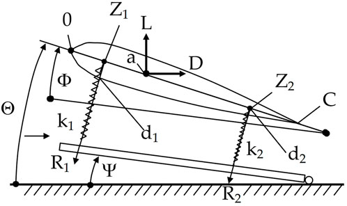
FIGURE 1. Coupled aerodynamics-structures system.

FIGURE 2

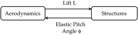
FIGURE 2. Block diagram of the coupled aerodynamics-structures system.

In the first part of this numerical experiment, in order to ensure that the coupling between the disciplines is satisfied in our proposed state-space Markov model, we compare our dynamic model with the Gibbs sampling process (Geman and Geman, 1984) which is a common approach in the analysis of coupled multidisciplinary systems. As it can be seen in Figure 3, the stationary distribution of the coupling variables achieved by our dynamic analysis is statistically similar to the one achieved by the Gibbs sampling process.

FIGURE 3

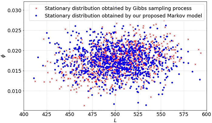
FIGURE 3. The particles representing the stationary distributions obtained by the Gibbs sampling process (red) and our proposed Markov model (blue).

In the following experiments, the impacts of state noise, measurement noise, initial state distribution, and measured state variables on the performance achieved in the state estimation process are studied. In all the experiments, synthetic state trajectories are generated and the root mean squared error between the estimated state at time step k (${\widehat{L}}_k$ and ${\widehat{\varphi }}_k$) and the true state (L_k and ϕ_k) is computed at each time step. These results are obtained over 100 independent runs of the particle filtering scheme. The root mean squared errors in different experiments are presented for comparison.

4.1.1 State noise

In this part of numerical experiments, the effect of state noise on the state estimation performance is investigated. We consider the following state noises:

$\begin{array}{cc}\hfill & \text{State\hspace{0.17em}Noise\hspace{0.17em}}1\text{:}{\sigma }_{v_L}^2=10{\sigma }_{v_{\varphi }}^2=10^{-8}\hfill \\ \hfill & \text{State\hspace{0.17em}Noise\hspace{0.17em}}2\text{:}{\sigma }_{v_L}^2=100{\sigma }_{v_{\varphi }}^2=10^{-6}\hfill \end{array}$

The number of particles is set to 10,000, the variances of measurement noises are ${\sigma }_{w_L}^2=10$ and ${\sigma }_{w_{\varphi }}^2=10^{-8}$, and the initial state distribution π₀ is considered to be:

$\mathcal{N}\left(\left[\begin{array}{c}\hfill 1000\hfill \\ \hfill 1\hfill \end{array}\right],\left[\begin{array}{cc}\hfill 100\hfill & \hfill 0\hfill \\ \hfill 0\hfill & \hfill 0.1\hfill \end{array}\right]\right).$

Figure 4 shows the average results obtained for the state noises. It can be seen that a larger state noise results in lower performance of state estimation. This is due to the higher stochasticity in the state process that makes the estimation process more challenging. The error curves for both state noises show a decreasing trend, which indicates that the state estimates become arbitrarily close to the true values for a sufficiently long time.

FIGURE 4

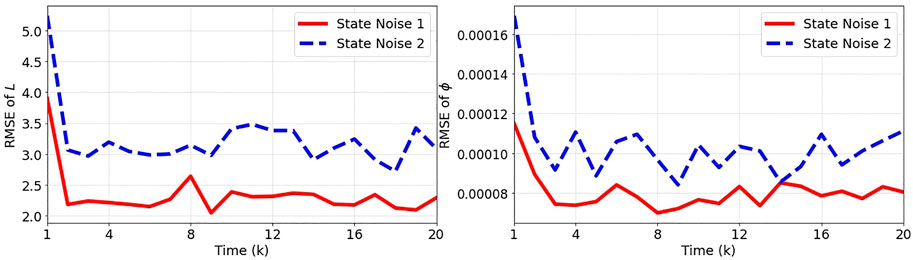
FIGURE 4. The root mean squared error (RMSE) between the true and estimated states L and ϕ over 100 independent runs for State Noise 1: ${\sigma }_{v_L}^2=10,{\sigma }_{v_{\varphi }}^2=10^{-8}$ and State Noise 2: ${\sigma }_{v_L}^2=100,{\sigma }_{v_{\varphi }}^2=10^{-6}$.

4.1.2 Measurement noise

In this part, the effect of measurement noise on the performance of state estimation is investigated. For this analysis, we consider the following measurement noises:

$\begin{array}{cc}\hfill & \text{Measurement\hspace{0.17em}Noise\hspace{0.17em}}1\text{:}{\sigma }_{w_L}^2=10{\sigma }_{w_{\varphi }}^2=10^{-8}\hfill \\ \hfill & \text{Measurement\hspace{0.17em}Noise\hspace{0.17em}}2\text{:}{\sigma }_{w_L}^2=100{\sigma }_{w_{\varphi }}^2=10^{-4}\hfill \end{array}$

The number of particles is 10,000, the variances of state noises are set to ${\sigma }_{v_L}^2=10$ and ${\sigma }_{v_{\varphi }}^2=10^{-8}$, and the initial state distribution π₀ is considered to be:

$\mathcal{N}\left(\left[\begin{array}{c}\hfill 1000\hfill \\ \hfill 1\hfill \end{array}\right],\left[\begin{array}{cc}\hfill 100\hfill & \hfill 0\hfill \\ \hfill 0\hfill & \hfill 0.1\hfill \end{array}\right]\right).$

Figure 5 shows the results obtained over 100 independent runs for the two considered measurement noises. As expected, the performance of state estimation significantly decreases with the increase in the measurement noise. This can be seen by the higher error of state estimation for the case of measurement noise 2.

FIGURE 5

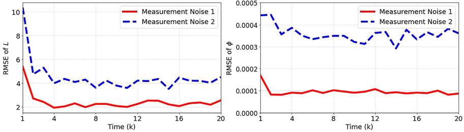
FIGURE 5. The root mean squared error (RMSE) between the true and estimated states L and ϕ over 100 independent runs for Measurement Noise 1: ${\sigma }_{w_L}^2=10,{\sigma }_{w_{\varphi }}^2=10^{-8}$ and Measurement Noise 2: ${\sigma }_{w_L}^2=100,{\sigma }_{w_{\varphi }}^2=10^{-4}$.

4.1.3 Initial state distribution

In this part of numerical experiments, we study the impact of initial state distribution, π₀, on the performance of state estimation. We consider two initial distributions:

$\begin{array}{cc}\hfill & {\pi }_0^1:\mathcal{N}\left(\left[\begin{array}{c}\hfill 1000\hfill \\ \hfill 1\hfill \end{array}\right],\left[\begin{array}{cc}\hfill 10\hfill & \hfill 0\hfill \\ \hfill 0\hfill & \hfill 0.01\hfill \end{array}\right]\right)\hfill \\ \hfill & {\pi }_0^2:\mathcal{N}\left(\left[\begin{array}{c}\hfill 1000\hfill \\ \hfill 1\hfill \end{array}\right],\left[\begin{array}{cc}\hfill 100\hfill & \hfill 0\hfill \\ \hfill 0\hfill & \hfill 0.1\hfill \end{array}\right]\right)\hfill \end{array}$

The number of particles is 10,000, the variances of state noises are ${\sigma }_{v_L}^2=10$ and ${\sigma }_{v_{\varphi }}^2=10^{-8}$, and the variances of measurement noises are ${\sigma }_{w_L}^2=10$ and ${\sigma }_{w_{\varphi }}^2=10^{-8}$. Figure 6 shows the average results for the two initial state distributions. It can be seen that the tighter initial distribution results in better state estimation in the first time steps. The difference in the performance in the early steps arises from the distribution of initial particles and this difference disappears as more measurements are available for the state estimation.

FIGURE 6

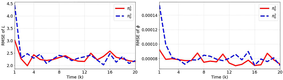
FIGURE 6. The root mean squared error (RMSE) between the true and estimated states L and ϕ over 100 independent runs for two initial state distributions ${\pi }_0^1$ and ${\pi }_0^2$.

4.1.4 Measured state variables

In this part, we study the impact of measuring only part of the states on the performance achieved by the particle filter. We consider three cases of measuring only L, measuring ϕ, and measuring both L and ϕ. For this analysis, the number of particles is 10,000, the variances of state noises are ${\sigma }_{v_L}^2=10$ and ${\sigma }_{v_{\varphi }}^2=10^{-8}$, and the variances of measurement noises are ${\sigma }_{w_L}^2=10$ and ${\sigma }_{w_{\varphi }}^2=10^{-8}$ and the initial state distribution π₀ is considered to be:

$\mathcal{N}\left(\left[\begin{array}{c}\hfill 1000\hfill \\ \hfill 1\hfill \end{array}\right],\left[\begin{array}{cc}\hfill 100\hfill & \hfill 0\hfill \\ \hfill 0\hfill & \hfill 0.1\hfill \end{array}\right]\right).$

Figure 7 shows the results obtained for these three cases. As expected, measuring both L and ϕ results in a good state estimation performance as it provides the highest information about the system. Once we measure only one of the state variables L or ϕ, the estimation error associated with the measured variable is minimum and the error associated with the other state variable is high. However, it can be seen that each of the measured state variables provides information for the estimation of the other state variable due to the correlations that exist between the two variables.

FIGURE 7

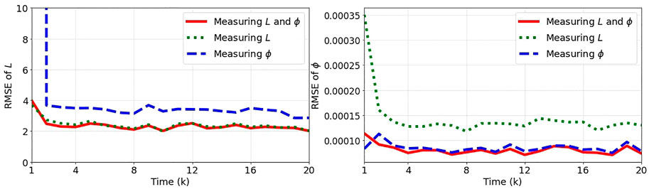
FIGURE 7. The root mean squared error (RMSE) between the true and estimated states L and ϕ over 100 independent runs for cases of measuring both or only one of the state variables.

4.2 Three-discipline fire detection satellite model

In this part, the SIR particle filter is analyzed on state estimation in a fire detection satellite model originally described in (Larson and Wertz, 1992). This is a hypothetical but realistic spacecraft consisting of a large number of disciplines with both feedback and feed-forward couplings. Here, we consider the modified version of this problem consisting of a subset of three disciplines considered earlier by Chaudhuri et al. (2017) and Sankararaman and Mahadevan (2012). This modified multidisciplinary system consists of Orbit, Attitude Control, and Power disciplines, illustrated in Figure 8. The primary objective of this satellite is to detect, identify, and monitor forest fires in near real time. This satellite is intended to carry a large and accurate optical sensor of length 3.2 m, weight 720 kg and has an angular resolution of 8.8 × 10⁻⁷ radians. As seen in Figure 8, the Orbit discipline has feed-forward coupling with both Attitude Control and Power disciplines, whereas the Attitude Control and Power disciplines have feedback or bidirectional coupling through three variables. These coupling variables are the attitude control system power (P^ACS) and the maximum and minimum moment of inertia of the spacecraft (I^max and I^min), considered as the state variables. The system model that is the functional relationships between the state variables is as follows:

$\begin{array}{cc}\hfill P_k^{\mathit{ACS}}=& {\omega }^{\mathit{max}}\max \left(\frac{4{\theta }^{\mathit{slew}}}{{\left(\mathrm{\Delta }{t}^{\mathit{slew}}\right)}^2}{I}_{k-1}^{\mathit{max}},\right.\hfill \\ \hfill & \left.\sqrt{{\left(\frac{3\mu |I_{k-1}^{\mathit{max}}-I_{k-1}^{\mathit{min}}|\sin \left(2\theta \right)}{2{\left(R^E+H_{k-1}\right)}^3}\right)}^2+{\left(L^{sp}\frac{F^S}{C}{A}^S\left(1+q\right)\cos \left(i\right)\right)}^2+{\left(\frac{2M{R}^D}{{\left(R^E+H_{k-1}\right)}^3}\right)}^2+{\left(\frac{1}{2}{L}^a\rho C^{d}A{v}^2\right)}^2}\right)\hfill \\ \hfill & +n{P}^{\mathit{hold}}+v_{1,k},\hfill \end{array}(19)$

$\begin{array}{ll}\hfill I_k^{\mathit{max}}=& \max \left(2{\rho }^{sa}\sqrt{\frac{f\left(P_{k-1}^{\mathit{ACS}}\right)r^{lw}}{n^{sa}}}\sqrt{\frac{f\left(P_{k-1}^{\mathit{ACS}}\right)}{r^{lw}{n}^{sa}}}t\left(\frac{1}{12}\left(\frac{f\left(P_{k-1}^{\mathit{ACS}}\right)r^{lw}}{n^{sa}}+t^2\right)+{\left(D+\frac{1}{2}\sqrt{\frac{\left(P_{k-1}^{\mathit{ACS}}\right)r^{lw}}{n^{sa}}}\right)}^2\right)\right.\hfill \\ \hfill & +I^{bod{y}_X},\frac{2}{12}{\rho }^{sa}\sqrt{\frac{f\left(P_{k-1}^{\mathit{ACS}}\right)r^{lw}}{n^{sa}}}\sqrt{\frac{f\left(P_{k-1}^{\mathit{ACS}}\right)}{r^{lw}{n}^{sa}}}t\left(t^2+\frac{f\left(P_{k-1}^{\mathit{ACS}}\right)}{r^{lw}{n}^{sa}}\right)\hfill \\ \hfill & +I^{bod{y}_Y},2{\rho }^{sa}\sqrt{\frac{f\left(P_{k-1}^{\mathit{ACS}}\right)r^{lw}}{n^{sa}}}\sqrt{\frac{f\left(P_{k-1}^{\mathit{ACS}}\right)}{r^{lw}{n}^{sa}}}t\left(\frac{1}{12}\left(\frac{f\left(P_{k-1}^{\mathit{ACS}}\right)r^{lw}}{n^{sa}}+\frac{f\left(P_{k-1}^{\mathit{ACS}}\right)}{r^{lw}{n}^{sa}}\right)\right.\left.\left.+{\left(D+\frac{1}{2}\sqrt{\frac{f\left(P_{k-1}^{\mathit{ACS}}\right)r^{lw}}{n^{sa}}}\right)}^2\right)+I^{bod{y}_Z}\right)+v_{2,k},\hfill \end{array}(20)$

$\begin{array}{ll}\hfill I_k^{\mathit{min}}=& \min \left(2{\rho }^{sa}\sqrt{\frac{f\left(P_{k-1}^{\mathit{ACS}}\right)r^{lw}}{n^{sa}}}\sqrt{\frac{f\left(P_{k-1}^{\mathit{ACS}}\right)}{r^{lw}{n}^{sa}}}t\left(\frac{1}{12}\left(\frac{f\left(P_{k-1}^{\mathit{ACS}}\right)r^{lw}}{n^{sa}}+t^2\right)+{\left(D+\frac{1}{2}\sqrt{\frac{\left(P_{k-1}^{\mathit{ACS}}\right)r^{lw}}{n^{sa}}}\right)}^2\right)\right.\hfill \\ \hfill & +I^{bod{y}_X},\frac{2}{12}{\rho }^{sa}\sqrt{\frac{f\left(P_{k-1}^{\mathit{ACS}}\right)r^{lw}}{n^{sa}}}\sqrt{\frac{f\left(P_{k-1}^{\mathit{ACS}}\right)}{r^{lw}{n}^{sa}}}t\left(t^2+\frac{f\left(P_{k-1}^{\mathit{ACS}}\right)}{r^{lw}{n}^{sa}}\right)\hfill \\ \hfill & +I^{bod{y}_Y},2{\rho }^{sa}\sqrt{\frac{f\left(P_{k-1}^{\mathit{ACS}}\right)r^{lw}}{n^{sa}}}\sqrt{\frac{f\left(P_{k-1}^{\mathit{ACS}}\right)}{r^{lw}{n}^{sa}}}t\left(\frac{1}{12}\left(\frac{f\left(P_{k-1}^{\mathit{ACS}}\right)r^{lw}}{n^{sa}}+\frac{f\left(P_{k-1}^{\mathit{ACS}}\right)}{r^{lw}{n}^{sa}}\right)\right.\left.\left.+{\left(D+\frac{1}{2}\sqrt{\frac{f\left(P_{k-1}^{\mathit{ACS}}\right)r^{lw}}{n^{sa}}}\right)}^2\right)+I^{bod{y}_Z}\right)+v_{3,k},\hfill \end{array}(21)$

where

${\theta }^{\mathit{slew}}=\arctan \left(\frac{\sin \left(\frac{{\varphi }^{\mathit{target}}}{R^E}\right)}{1-\cos \left(\frac{{\varphi }^{\mathit{target}}}{R^E}\right)+\frac{H}{R^E}}\right),$

$f\left(P^{\mathit{ACS}}\right)=\left(P^{\mathit{ACS}}+P^{\mathit{Other}}\right)\frac{\left(\frac{\mathrm{\Delta }{t}^{\mathit{eclipse}}}{0.6}+\frac{\left(\mathrm{\Delta }{t}^{\mathit{orbit}}-\mathrm{\Delta }{t}^{\mathit{eclipse}}\right)}{0.8}\right)}{\left(\mathrm{\Delta }{t}^{\mathit{orbit}}-\mathrm{\Delta }{t}^{\mathit{eclipse}}\right)\eta F^S{I}^l\cos \left(i\right){\left(1-{ϵ}^{\mathrm{deg}}\right)}^{LT}},$

$\mathrm{\Delta }{t}^{\mathit{orbit}}=2\pi \sqrt{\frac{{\left(R^E+H\right)}^3}{\mu }}=\frac{2\pi \left(R^E+H\right)}{v},\mathrm{\Delta }{t}^{\mathit{eclipse}}=\frac{\mathrm{\Delta }{t}^{\mathit{orbit}}}{\pi }\arcsin \left(\frac{R^E}{R^E+H}\right),v=\sqrt{\frac{\mu }{R^E+H}},$

and $v_{1,k}\sim \mathcal{N}(\mathrm{0,10})$, $v_{2,k}\sim \mathcal{N}(\mathrm{0,50})$, and $v_{3,k}\sim \mathcal{N}(\mathrm{0,50})$. Altitude (H) is the time-varying input to the system, that is:

$H_k=18\times 10^6+2\times 10^6\times \sin \left(\frac{k\pi }{10}\right).(22)$

FIGURE 8

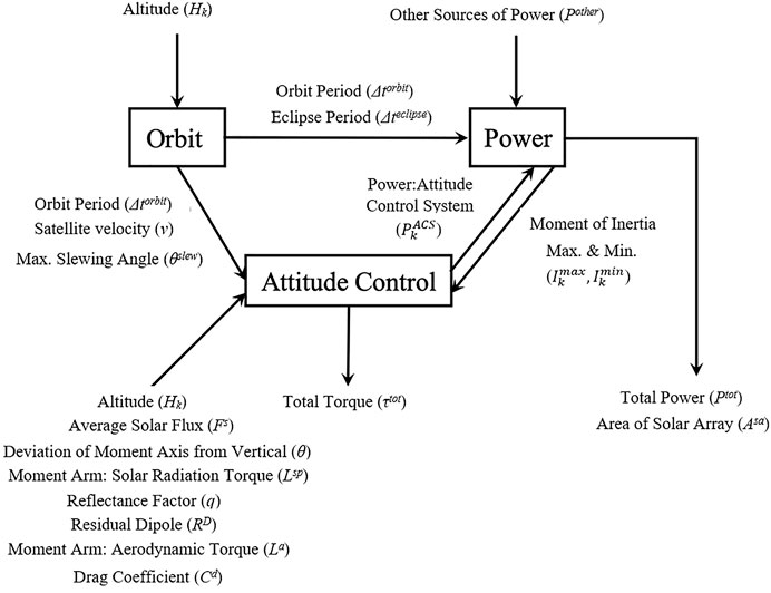
FIGURE 8. Three-discipline fire detection satellite.

The values associated with the variables in the system model are provided in Table 1. The states are partially observable through noisy measurements as:

${\mathbf{z}}_k=\left[\begin{array}{c}\hfill P_k^{\mathit{ACS}}+w_{1,k}\hfill \\ \hfill I_k^{\mathit{max}}+w_{2,k}\hfill \\ \hfill I_k^{\mathit{min}}+w_{3,k}\hfill \end{array}\right],$

where $w_{1,k}\sim \mathcal{N}(\mathrm{0,1})$, $w_{2,k}\sim \mathcal{N}(\mathrm{0,5})$, and $w_{3,k}\sim \mathcal{N}(\mathrm{0,5})$.

TABLE 1

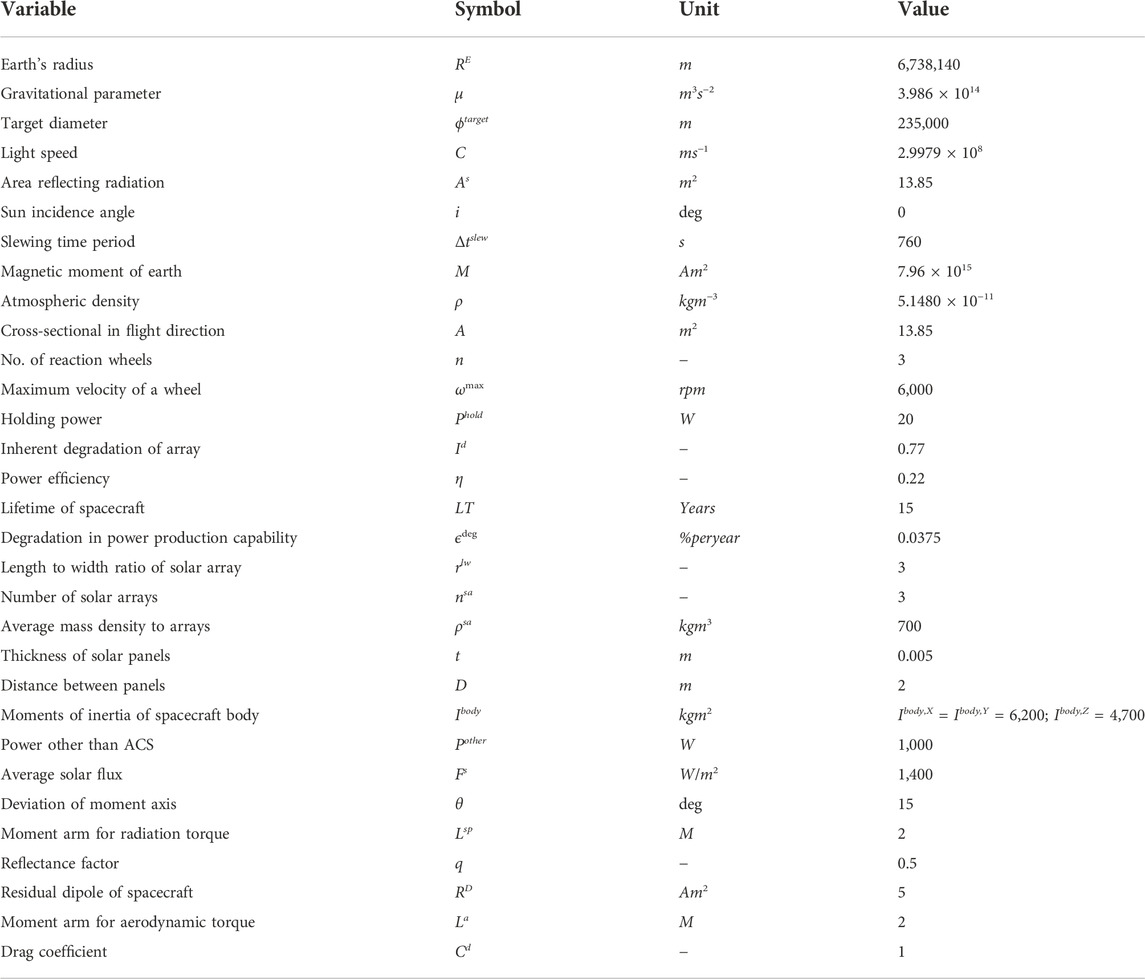
TABLE 1. List of variables in the fire detection satellite problem.

In this problem, we study the impact of different sensor measurements on the estimation of the state variables. Like the previous experiment, we generate synthetic state trajectories and perform the state estimation for 100 independent runs. We compare the results obtained by the particle filter in different cases of sensor measurements, when the measurements are from each state variable P^ACS, I^max, I^min and all the state variables denoted by X. For this analysis, the number of particles is set to 100,000, and the initial state distribution π₀ is considered to be:

$\mathcal{N}\left(\left[\begin{array}{c}\hfill 50\hfill \\ \hfill 1000\hfill \\ \hfill 1000\hfill \end{array}\right],\left[\begin{array}{ccc}\hfill 10\hfill & \hfill 0\hfill & \hfill 0\hfill \\ \hfill 0\hfill & \hfill 100\hfill & \hfill 0\hfill \\ \hfill 0\hfill & \hfill 0\hfill & \hfill 100\hfill \end{array}\right]\right).$

Figure 9 shows the root mean squared errors between the estimated states at time step k (${\widehat{P}}_k^{\mathit{ACS}}$, ${\widehat{I}}_k^{\mathit{max}}$, and ${\widehat{I}}_k^{\mathit{min}}$) and the true states ($P_k^{\mathit{ACS}}$, $I_k^{\mathit{max}}$, and $I_k^{\mathit{min}}$) at each time step for different measured variables. As expected, measuring all states together results in a good state estimation performance as they provide the highest information about the system. The results demonstrate that when we measure only one of the state variables P^ACS, I^max, or I^min, the estimation error associated with the measured variable is minimum and the errors associated with the other state variables are high. However, it can be seen that each of the measured state variables provides information for the estimation of the other state variables due to the correlations existing between the variables.

FIGURE 9

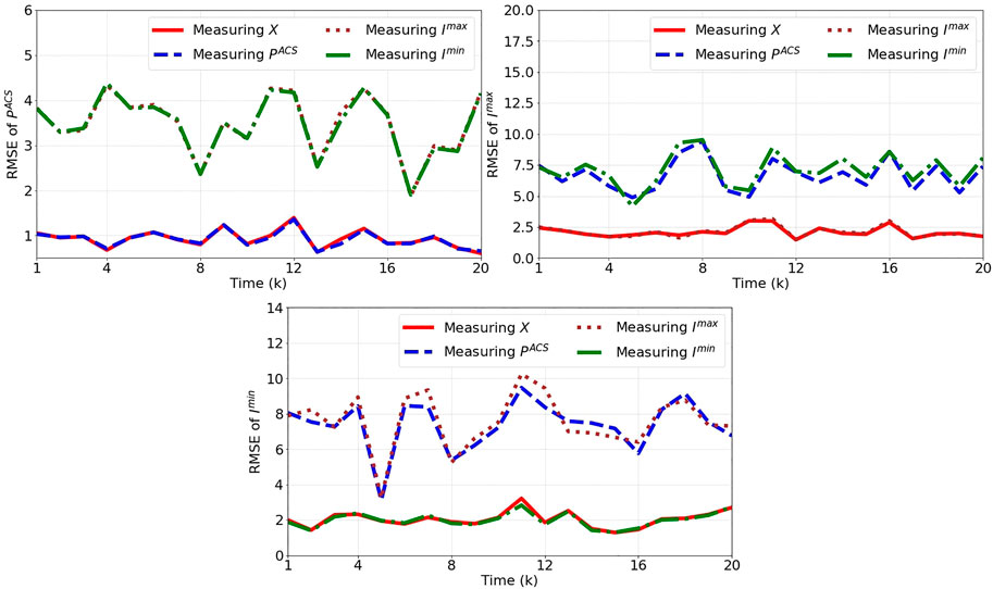
FIGURE 9. The root mean squared error (RMSE) between the true and estimated states over 100 independent runs for cases of measuring all or only one of the state variables.

5 Conclusion

Coupled multidisciplinary systems that are common in many engineering and science applications, consist of several disciplines interacting with each other. In most previous literature, the stationary state of coupled multidisciplinary systems has been studied without considering the time-varying interaction of the disciplines. However, the transient behavior of these systems in real-world applications is of great importance. In this paper, we studied the dynamic transition (i.e., the time-varying interaction of disciplines) in coupled multidisciplinary systems as opposed to their stationary behavior. The transient interactions between the disciplines can put the system at risk if the temporal evolution of the disciplines is not accounted for in the system’s design, control, and reliability analysis. To analyze this transient behavior, we presented a Markov state-space modeling of coupled multidisciplinary systems. By having this state-space formulation, we developed a particle filtering scheme for the state estimation of these complex multidisciplinary systems. Assuming that we have noisy observations from all or some of the disciplines, we investigated the impact of stochasticities and sensor measurements on the estimation process. The accurate estimation of the states through imperfect measurements is an essential step in the dynamic analysis of multidisciplinary systems to achieve reliable decision-making in their operation, considering each discipline’s constraints and preventing any severe damage once interacting with each other.

Data availability statement

The original contributions presented in the study are included in the article/supplementary material, further inquiries can be directed to the corresponding author.

Author contributions

NA developed the state-space modeling and the state estimation process, performed the experiments, and wrote the manuscript. SG oversaw the project, proposed the new state-space modeling and state estimation method, and wrote the manuscript. Both authors have read and approved the final manuscript.

Conflict of interest

The authors declare that the research was conducted in the absence of any commercial or financial relationships that could be construed as a potential conflict of interest.

Publisher’s note

All claims expressed in this article are solely those of the authors and do not necessarily represent those of their affiliated organizations, or those of the publisher, the editors and the reviewers. Any product that may be evaluated in this article, or claim that may be made by its manufacturer, is not guaranteed or endorsed by the publisher.

References

Agarwal, H., Renaud, J. E., Preston, E. L., and Padmanabhan, D. (2004). Uncertainty quantification using evidence theory in multidisciplinary design optimization. Reliab. Eng. Syst. Saf. 85, 281–294. doi:10.1016/j.ress.2004.03.017

CrossRef Full Text | Google Scholar

Agarwal, H., and Renaud, J. (2004). Reliability based design optimization using response surfaces in application to multidisciplinary systems. Eng. Optim. 36, 291–311. doi:10.1080/03052150410001666578

CrossRef Full Text | Google Scholar

Arulampalam, M. S., Maskell, S., Gordon, N., and Clapp, T. (2002). A tutorial on particle filters for online nonlinear/non-Gaussian bayesian tracking. IEEE Trans. Signal Process. 50, 174–188. doi:10.1109/78.978374

CrossRef Full Text | Google Scholar

Asadi, N., and Ghoreishi, S. F. (2022). “Input distribution estimation in dynamic coupled multidisciplinary systems,” in 2022 56th Asilomar Conference on Signals, Systems, and Computers (Piscataway, NJ, USA: IEEE).

Google Scholar

Chaudhuri, A., Lam, R., and Willcox, K. (2017). Multifidelity uncertainty propagation via adaptive surrogates in coupled multidisciplinary systems. AIAA J. 56, 235–249. doi:10.2514/1.j055678

CrossRef Full Text | Google Scholar

Cramer, E. J., Dennis, J. E., Frank, P. D., Lewis, R. M., and Shubin, G. R. (1994). Problem formulation for multidisciplinary optimization. SIAM J. Optim. 4, 754–776. doi:10.1137/0804044

CrossRef Full Text | Google Scholar

Culler, A. J., and McNamara, J. J. (2010). Studies on fluid-thermal-structural coupling for aerothermoelasticity in hypersonic flow. AIAA J. 48, 1721–1738. doi:10.2514/1.j050193

CrossRef Full Text | Google Scholar

Doucet, A., and Johansen, A. M. (2009). A tutorial on particle filtering and smoothing: Fifteen years later. Handb. nonlinear Filter. 12, 3.

Google Scholar

Du, X., and Chen, W. (2005). Collaborative reliability analysis under the framework of multidisciplinary systems design. Optim. Eng. 6, 63–84. doi:10.1023/b:opte.0000048537.35387.fa

CrossRef Full Text | Google Scholar

Du, X., Guo, J., and Beeram, H. (2008). Sequential optimization and reliability assessment for multidisciplinary systems design. Struct. Multidiscipl. Optim. 35, 117–130. doi:10.1007/s00158-007-0121-7

CrossRef Full Text | Google Scholar

Dunning, P. D., Kim, H. A., and Mullineux, G. (2011). Introducing loading uncertainty in topology optimization. AIAA J. 49, 760–768. doi:10.2514/1.j050670

CrossRef Full Text | Google Scholar

Friedman, S., Ghoreishi, S. F., and Allaire, D. L. (2017). “Quantifying the impact of different model discrepancy formulations in coupled multidisciplinary systems,” in 19th AIAA non-deterministic approaches conference, 1950.

CrossRef Full Text | Google Scholar

Friedman, S., Isaac, B., Ghoreishi, S. F., and Allaire, D. L. (2018). “Efficient decoupling of multiphysics systems for uncertainty propagation,” in 2018 AIAA Non-Deterministic Approaches Conference, 1661.

CrossRef Full Text | Google Scholar

Geman, S., and Geman, D. (1984). Stochastic relaxation, gibbs distributions, and the bayesian restoration of images. IEEE Trans. Pattern Anal. Mach. Intell. 1984, 721–741. doi:10.1109/tpami.1984.4767596

PubMed Abstract | CrossRef Full Text | Google Scholar

Ghoreishi, S., and Allaire, D. (2017). Adaptive uncertainty propagation for coupled multidisciplinary systems. AIAA J. 55, 3940–3950. doi:10.2514/1.j055893

CrossRef Full Text | Google Scholar

Ghoreishi, S. F., and Allaire, D. L. (2016). “Compositional uncertainty analysis via importance weighted gibbs sampling for coupled multidisciplinary systems,” in 18th AIAA non-deterministic approaches conference, 1443.

CrossRef Full Text | Google Scholar

Ghoreishi, S. F., and Imani, M. (2020). “Bayesian optimization for efficient design of uncertain coupled multidisciplinary systems,” in 2020 American Control Conference (ACC) (Denver, CO, USA: IEEE), 3412–3418. doi:10.23919/ACC45564.2020.9147526

CrossRef Full Text | Google Scholar

Ghoreishi, S. F., and Imani, M. (2021). Bayesian surrogate learning for uncertainty analysis of coupled multidisciplinary systems. J. Comput. Inf. Sci. Eng. 21. doi:10.1115/1.4049994

CrossRef Full Text | Google Scholar

Ghoreishi, S. F. (2016). Uncertainty analysis for coupled multidisciplinary systems using sequential importance resampling. Master’s thesis.

Glynn, P. W., and Iglehart, D. L. (1989). Importance sampling for stochastic simulations. Manag. Sci. 35, 1367–1392. doi:10.1287/mnsc.35.11.1367

CrossRef Full Text | Google Scholar

Gordon, N. J., Salmond, D. J., and Smith, A. F. (1993). Novel approach to nonlinear/non-Gaussian Bayesian state estimation. Radar Signal Process. IEE Proc. F (IET) 140, 107–113. doi:10.1049/ip-f-2.1993.0015

CrossRef Full Text | Google Scholar

Gu, X., Renaud, J. E., Batill, S. M., Brach, R. M., and Budhiraja, A. S. (2000). Worst case propagated uncertainty of multidisciplinary systems in robust design optimization. Struct. Multidiscipl. Optim. 20, 190–213. doi:10.1007/s001580050148

CrossRef Full Text | Google Scholar

Guo, J., and Du, X. (2010). Reliability analysis for multidisciplinary systems with random and interval variables. AIAA J. 48, 82–91. doi:10.2514/1.39696

CrossRef Full Text | Google Scholar

Hart, C. G., and Vlahopoulos, N. (2010). An integrated multidisciplinary particle swarm optimization approach to conceptual ship design. Struct. Multidiscipl. Optim. 41, 481–494. doi:10.1007/s00158-009-0414-0

CrossRef Full Text | Google Scholar

Hearn, T. A., Hendricks, E., Chin, J., and Gray, J. S. (2016). “Optimization of turbine engine cycle analysis with analytic derivatives,” in 17th AIAA/ISSMO Multidisciplinary Analysis and Optimization Conference, 4297.

CrossRef Full Text | Google Scholar

Larson, W. J., and Wertz, J. R. (1992). Space mission analysis and design. Tech. rep. Torrance, CA, USA: Microcosm, Inc.

Google Scholar

Meng, D., Li, Y. F., Huang, H. Z., Wang, Z., and Liu, Y. (2015). Reliability-based multidisciplinary design optimization using subset simulation analysis and its application in the hydraulic transmission mechanism design. J. Mech. Des. 137, 051402. doi:10.1115/1.4029756

CrossRef Full Text | Google Scholar

Sankararaman, S., and Mahadevan, S. (2012). Likelihood-based approach to multidisciplinary analysis under uncertainty. J. Mech. Des. 134, 031008. doi:10.1115/1.4005619

CrossRef Full Text | Google Scholar

Smith, A. F., and Gelfand, A. E. (1992). Bayesian statistics without tears: A sampling–resampling perspective. Am. Statistician 46, 84–88. doi:10.2307/2684170

CrossRef Full Text | Google Scholar

Sobieszczanski-Sobieski, J., and Haftka, R. T. (1997). Multidisciplinary aerospace design optimization: Survey of recent developments. Struct. Optim. 14, 1–23. doi:10.1007/bf01197554

CrossRef Full Text | Google Scholar

Sobieszczanski-Sobieski, J. (1990). Sensitivity of complex, internally coupled systems. AIAA J. 28, 153–160. doi:10.2514/3.10366

CrossRef Full Text | Google Scholar

Yao, W., Chen, X., Luo, W., Van Tooren, M., and Guo, J. (2011). Review of uncertainty-based multidisciplinary design optimization methods for aerospace vehicles. Prog. Aerosp. Sci. 47, 450–479. doi:10.1016/j.paerosci.2011.05.001

CrossRef Full Text | Google Scholar

Zaman, K., and Mahadevan, S. (2013). Robustness-based design optimization of multidisciplinary system under epistemic uncertainty. Aiaa J. 51, 1021–1031. doi:10.2514/1.j051372

CrossRef Full Text | Google Scholar

Jiaqiang, E., Gong, J., Yuan, W., Zuo, W., Li, Y., et al. (2016a). Multidisciplinary design optimization of the diesel particulate filter in the composite regeneration process. Appl. energy 181, 14–28. doi:10.1016/j.apenergy.2016.08.051

CrossRef Full Text | Google Scholar

Zhang, M., Gou, W., Li, L., Wang, X., and Yue, Z. (2016b). Multidisciplinary design and optimization of the twin-web turbine disk. Struct. Multidiscipl. Optim. 53, 1129–1141. doi:10.1007/s00158-015-1373-2

CrossRef Full Text | Google Scholar