A multi-fidelity model management framework for multi-objective aerospace design optimisation

1 Introduction

The usability of systems-based multidisciplinary design optimisation is often dependant on the extent to which complex interdisciplinary interactions can be represented. Practical boundaries on computational resource naturally limit subsystem modelling towards inexpensive, less accurate and/or flexible numerical/empirical methods. Performance predictions may thus be misleading, failing to represent significant design behaviour or interdisciplinary coupling (Christensen and Willcox, 2012; Robinson, 2012; Bryson et al., 2019). This can ultimately lead to sub-optimal designs and/or increased development costs as a result of later stage alteration (Allaire and Willcox, 2014).

Multi-fidelity¹ (MF) meta-modelling has become a popular means of efficiently distributing computational resource across various levels of simulation accuracy. In this manner, one may obtain numerically accurate predictions of an expensive function response whilst minimising the associated cost penalty (Fernandez et al., 2017; Park et al., 2017; Liu et al., 2018). Such methods have found wide application, particularly within the field of surrogate based optimisation (SBO). Approaches include utilising low-fidelity (LF) models to accelerate the search for the global optimum (Booker et al., 1999; Keane, 2003; Forrester and Keane, 2009), leveraging an adaptively corrected LF model within a trust region model management scheme (Alexandrov et al., 1997; 2001; Booker et al., 1999; March and Willcox, 2012b), or directly optimising a MF approximation of the objective function. A well known example of the latter is efficient global optimisation (EGO), which optimises a Kriging approximation constructed from evaluations of the “true” objective function (Jones et al., 1998).

Techniques for MF model management (including methods for general model enhancement, out-with any overriding outer-loop application) may be described according to the following classifications (Peherstorfer et al., 2018); adaptation, fusion and filtering. Adaptation refers to directly correcting or enhancing an existing LF model (or set of models) using selective samples of a correlated, high(er)-fidelity model. Common forms of adaptive correction include bridge functions (additive, multiplicative or comprehensive) (Gano et al., 2005; Han et al., 2013; Fischer et al., 2018), model calibration (Kennedy and O’Hagan, 2001; March and Willcox, 2012a) and space mapping (Bandler et al., 1994; Koziel et al., 2008). Fusion instead involves the combination of separate levels of fidelity into a single surrogate (Forrester et al., 2007; Zhou et al., 2019). For example, the work presented by Allaire and Willcox (2014) approximates each level of fidelity via a separate kriging surrogate, before the technique presented by Winkler (1981) is used to combine the random variables associated with each kriging approximation, thus producing a single fused model. Furthermore, this method may also be applied by averaging the response of an ensemble of meta-models, such as in the work Goel et al. (2007), where model weights are derived from their respective error profiles. Filtering refers to a hierarchical management of models, or surrogates thereof. For example, evaluating the HF function only when the LF counterpart falls outwith a certain acceptable accuracy, or when some specific criteria are met (Fernández-Godino et al., 2016). This classification also includes multilevel methods (inc. multigird methods, multilevel pre-conditioners and multilevel function representations). The reader is referred to the following reviews for in-depth analyses and examples of MF modelling applications (Huang et al., 2013; Fernández-Godino et al., 2016; Koziel and Leifsson, 2016; Peherstorfer et al., 2018).

Multi-stage approaches to adaptive model correction have received some attention in the literature. In most cases, one or more correction methods are implemented as pre-processing stages to improve the prediction quality of the final surrogate. Park et al. (2018) report that the use of scaling coefficients to reduce the “bumpiness” (an integral of the square of the second derivative) of the discrepancy function can increase the prediction accuracy of the final stage surrogate. Koziel and Leifsson (2012) present a multi-point space mapping method, a generalised update to Output Space Mapping (OSM), as a multi-stage corrective procedure using a constant linear scaling function as a precursor to a direct correction via additive discrepancy, calculated using the first stage output.

This work presents a simple exploration of this concept, and incorporates the resulting methodology into a multidisciplinary design optimisation process. In the proposed approach, phase specific/invariant LF physics-based subsystem models are adaptively and iteratively corrected via several distinct parametric/non-parametric stages. Globally approximating surrogates are constructed at each degree of fidelity (low, mid, and high) via an automated hyper-parameter selection and training procedure. The resulting hierarchy drives the optimisation process, with local refinement managed according to a confidence-based multi-response adaptive sampling procedure, with bias given to global parameter sensitivities.

The overarching goal of this work is to contribute in part to a generalised framework supporting MF optimisation and optimal control problems. Surrogate generation and data correction methods are implemented within a modular outer-level structure. Each subroutine is designed to be applicable in a general sense, to enhance the flexibility and applicability of the framework. For example, multiple alternative/competing models may be specified for a particular subsystem. Models themselves may have non-equal (or overlapping) input domains, and may be time-phase specific or shared across multiple phases. Sample points at which models are to be initially evaluated may be supplied, or autonomously selected via the proposed surrogate generation procedure. Additionally, existing data may be supplied to augment the model generation process as sets of corresponding input/output arrays.

The remainder of this paper is organised as follows. Section 2 briefly details the surrogate generation technique employed. Section 3 details the series of response correction stages, then Sections 4, 5 demonstrate their application to an isolated engineering test case. The completed framework, including surrogate generation and adaptation processes, is then used to solve a set of single-objective optimisation problems (Sections 6, 7). Section 8 presents the associated cost savings, and finally, Section 9 presents the author’s conclusions and recommendations.

2 Surrogate generation

Considering the generation of surrogate models (SM) for use within optimisation and optimal control problems, the goal is often to provide a global representation of the HF response meeting the requirements of zero- and first-order consistency (Alexandrov et al., 2001) to an acceptable degree within a reduced computational budget. The latter point is as compared with constructing a surrogate of similar accuracy using exclusive HF sampling. First order consistency is desirable (though not always achievable) in this context given that, in conventional mathematics, if a surrogate and its derivative matches the target function, convergence to the same solution can be guaranteed (Alexandrov et al., 2001). Specifically considering continuous optimal control problems, it is highly desirable that system models are continuously differentiable given that a continuous/smooth representation of the dynamic system state is often required to reach feasible solutions.

Common methods of generating continuously differentiable SMs suited to MF applications are Kriging (Sacks et al., 1989) and Response Surface Modelling (Myers and Montgomery, 1995). However, these methods often require the user-specification of hyperparameters such as (in the case of Kriging) regression and correlation functions (including an initial guess of the correlation function parameters), which may require a priori knowledge of the function under consideration. Whilst for physics-based subsystem models a certain degree of domain specific knowledge may be assumed, the most appropriate choice of hyperparameters may not necessarily remain constant across separate subsystems. This work aims to implement a more generalised methodology, suitable for multiple models of unknown functional form within multiple subsystems.

Artificial Neural Networks (ANN) (McCulloch and Pitts, 1943) for non-linear regression are an appealing non-parametric alternative. An ANN is a multi-layered construction comprising one or more hidden layers of different processing units (neurons) that are connected to form a network. Each connection is characterised by a corresponding weight, iteratively adjusted by the training procedure, that defines the effect of each unit on the overall surrogate model. Whilst a typical multi-layer network may contain any number of hidden layers, it has been widely reported that an ANN with only one sigmoidal hidden layer (chosen due to being easily differentiable) and a linear output layer (to allow a non-bounded output) is capable of approximating any linear/non-linear function with a finite number of discontinuities to an arbitrary accuracy, provided that associated conditions are satisfied (Razavi et al., 2012; Beale et al., 2017; Rumelhart et al., 1994). Indeed, the work by Razavi et al. (2012) found that the use of more than one hidden layer in an ANN-based meta-modelling study was in itself extremely rare. An additional implication here is that one may employ an ANN based meta-modelling scheme without any prior knowledge of the underlying function to be approximated (Minisci and Vasile, 2013).

Throughout this work, continuously differentiable meta-models of single and multi-fidelity datasets are constructed by employing a generalised training methodology for multi-layer feed-forward ANN. This approach, largely adapted from the recommendations of Heath (2020), aims to programmatically determine the optimal hyperparameters of a standard Multi-Layer Perceptron (MLP) architecture as implied by the Kolmogorov theorem (Kolmogorov, 1957). This approach utilises both Bayesian Regularisation and an early-stopping criteria implemented using the MATLAB^Ⓡ Neural Network Toolbox (Beale et al., 2017). Designed analogous to a black-box function, sample sets are provided as input with the corresponding surrogate model(s) produced as output.

In this work, initial sample sets are generated using Latin Hypercube Sampling (LHS) to ensure that space-filling criteria can be met across the entire input domain for any sample size n_s. Within the proposed procedure, the input data is subsequently distributed amongst training, validation and testing sets, where the number of samples in each, n_trn, n_val and n_tst respectively, conforms to the following ratios:

$\left[\begin{array}{c}\hfill n_{\mathit{trn}}\hfill \\ \hfill n_{\mathit{val}}\hfill \\ \hfill n_{\mathit{tst}}\hfill \end{array}\right]=n_s\left[\begin{array}{c}\hfill {\varphi }_{\mathit{trn}}\hfill \\ \hfill {\varphi }_{\mathit{val}}\hfill \\ \hfill {\varphi }_{\mathit{tst}}\hfill \end{array}\right]=n_s\left[\begin{array}{c}\hfill 0.7\hfill \\ \hfill 0.15\hfill \\ \hfill 0.15\hfill \end{array}\right](1)$

The number of samples n_s for an input vector of dimension d_in is chosen such that:

$10d_{in}\le n_{\mathit{trn}}\le 30d_{in}(2)$

The number of unknown network parameters (e.g., weights and biases) N_w is given by:

$N_w=H\left(d_{in}+1\right)+d_{\mathit{out}}\left(H+1\right)(3)$

where H is the number of neurons in the single hidden layer. The number of training equations required for a given training set is given by:

$N_{\mathit{trneq}}=n_{\mathit{trn}}\ast d_{\mathit{out}}(4)$

where n_trn is consistent with Eq. 1. To avoid over-fitting,

$N_w\le N_{\mathit{trneq}}(5)$

From Eqs 3, 4 it is clear that Eq. 5 will always be true provided the number of neurons H is less than or equal to an upper bound H_ub:

$H_{ub}=⌈\frac{d_{\mathit{out}}\left(n_{\mathit{trn}}-1\right)}{d_{in}+d_{\mathit{out}}+1}⌉(6)$

To determine the appropriate network parameter values, an outer loop varies the number of neurons in the hidden layer, H, in 10 near-equally spaced divisions between a lower bound of 0 (representing a linear response) and the upper bound H_ub. A nested inner loop then performs 10 random initialisations of the network weights, biases and data divisions², before sequentially training each network to convergence. In each case, the objective is to determine the network parameters that yield an acceptable ratio of mean-square-error to mean-target-variance for random subsets of non-training data (Heath, 2020). Training performance is tracked via the network errors recorded for the independent testing set of size n_tst (Eq. 1). A normalised performance criteria relating N_t predictions α and targets t facilitates network selection:

$R^2=1-\frac{\frac{1}{N_t}{\sum }_{i=1}^{N_t}{\left(t_i-{\alpha }_i\right)}^2}{\frac{1}{N_t}{\sum }_{i=1}^{N_t}{\left(t_i-\bar{t}\right)}^2}(7)$

To reduce the risk of a poor generalisation (overfitting), it is of interest to minimise the number of neurons used within the hidden layer. A minimum performance criteria is defined as the successful modelling of 99% of the target subset variance (R² ≥ 0.99). Therefore, the network that achieves this criteria for a minimum number of hidden layer neurons is selected.

3 Methods

This section recalls the general formulation of the proposed multi-stage model correction process, originally presented in Parsonage and Maddock (2020), the initial surrogate generation process and the adaptive sampling procedure incorporated within the overall management framework.

3.1 Formulation

A generic model is defined as a function f: X → Y that for a given input x ∈ X produces an output y ∈ Y where $\mathbf{X}\subseteq {\mathbb{R}}^{d_{in}}$ is the input domain with dimension $d_{in}\subset \mathbb{N}$ and $\mathbf{Y}\subset {\mathbb{R}}^{d_{\mathit{out}}}$ is the output domain with dimension $d_{\mathit{out}}\subset \mathbb{N}$:

${\mathbf{x}}^{\left(i\right)}\mapsto {\mathbf{y}}^{\left(i\right)}=\mathbf{f}\left({\mathbf{x}}^{\left(i\right)}\right),i=\mathrm{1,2},\dots ,n_s(8)$

In this context, f(x) may represent the direct evaluation of a subsystem model or the evaluation of an appropriate surrogate approximation. Thus HF and LF models are notated simply as f_H: X → Y and f_L: X → Y, and a generic surrogate model as f_S: X → Y. Let x⁽ⁱ⁾, i = 1, …, M denote the set of M design points. Directly collocated samples are assumed, although such a correspondence may be obtained via surrogate estimation (Forrester et al., 2007). A nested set of N HF samples may thus be defined as ${\mathbf{x}}_H^{(j)}$, j = 1, …, N where x_H ∈ x.

3.2 Parameter extraction

An approximate relationship between two competing responses, f_L and f_H, (both of dimension d_out) can be defined as a quantifiable set of scaling parameters of the linear form (Koziel and Leifsson, 2016):

${\mathbf{f}}_S\left(\mathbf{x},\mathbf{p}\right)=\mathbf{a}{\mathbf{f}}_L\left(\mathbf{x}\right)+\mathbf{b}(9)$

where a and b are vectors of d_out unbounded scaling coefficients, and p(a, b) is found by formulating Eq. 9 into a parameter extraction sub-problem:

$\mathbf{p}=\arg \underset{\mathbf{q}}{\min }\frac{1}{\sigma }\sqrt{\frac{1}{N}\sum _{k=1}^N{\left[{\mathbf{f}}_S\left({\mathbf{x}}_H^{\left(k\right)},\mathbf{q}\right)-{\mathbf{f}}_H\left({\mathbf{x}}_H^{\left(k\right)}\right)\right]}^2}(10)$

where σ is the standard deviation of the samples ${\mathbf{x}}_H^{(k)}$. This method is referred to throughout this work as the Parametric (P) stage.

3.3 Response mapping

An alternate approach is to quantify the relative change in f_L between each pair-wise combination of M design points x and N samples x_H. The resulting translation matrix T is notated as:

${\mathbf{T}}_{i,j}={\mathbf{f}}_L\left({\mathbf{x}}^{\left(i\right)}\right)-{\mathbf{f}}_L\left({\mathbf{x}}_H^{\left(j\right)}\right)\left\{\begin{array}{c}i=1,\dots ,M\hfill \\ j=1,\dots ,N\hfill \end{array}\right.(11)$

The HF response at each design point x⁽ⁱ⁾ is predicted according to:

${\mathbf{f}}_S\left({\mathbf{x}}^{\left(i\right)}\right)=\frac{\sum {\left[\left({\mathbf{f}}_H\left({\mathbf{x}}_H^{\left(j\right)}\right)+{\mathbf{T}}_{i,j}\right)\ast {\mathbf{w}}_{i,j}\right]}_{j=1,\dots ,N}}{\sum {\left[{\mathbf{w}}_{i,j}\right]}_{j=1,\dots ,N}}(12)$

The weight factor w_i,j is dependant on the pairwise euclidean norms between x and x_H:

${\mathbf{w}}_{i,j}=1-\sqrt{\sum _{k=1}^{d_{in}}{\left[{\widehat{\mathbf{x}}}^{\left(i,k\right)}-{\widehat{\mathbf{x}}}_H^{\left(j,k\right)}\right]}^2}(13)$

where $\widehat{\mathbf{x}}$ denotes the scaled form of input x conforming to ${\widehat{\mathbf{x}}}^{(i,k)}\in [\mathrm{0,1}]$ for all k = 1, …, d_in. Similarly, ${\widehat{\mathbf{w}}}_{i,j}\in [\mathrm{0,1}]$. This method is referred to as the Relative (R) stage throughout the remainder of this paper.

3.4 Neural network bridge function

The final stage constructs a continuous ANN surrogate of the additive discrepancy between responses, defined as a set of translation vectors t:

${\mathbf{t}}_j={\mathbf{f}}_L\left({\mathbf{x}}_H^{\left(j\right)}\right)-{\mathbf{f}}_H\left({\mathbf{x}}_H^{\left(j\right)}\right),j=1,\dots ,N(14)$

To mitigate the effects of an insufficient input data on training performance, an augmented set of translation vectors $\tilde{\mathbf{t}}$ may be defined as:

$\tilde{\mathbf{t}}=\left[\mathbf{t},\mathbf{a}\right],{\mathbf{a}}_j={\mathbf{b}}_j+w{\mathit{\theta }}_j,j=1,\dots ,n_{\mathit{aug}}(15)$

where b ⊂ t, w is a scalar weighting factor (default 1%), θ is a vector of random values θ ∈ [−1, 1] and the number of augments n_aug = n_desired − N. The minimum input set size n_desired = 30d_in/ϕ_trn, where ϕ_trn is consistent with Eq. 1. The resulting set of translation vectors is mapped to a continuous function via the training procedure detailed in Section 2. Performance is additionally examined by evaluating the prediction accuracy obtained by applying the translation network across the original response data. The network exhibiting the strongest correction quality and training accuracy is selected. This method is referred to as the Additive (A) stage throughout the remainder of this work.

3.5 Initial surrogate generation

To begin, the above correction techniques are successively applied to a LF sample set selected using LHS and supplemented with a minimum of two samples of the expensive HF function (such that an output gradient may be observed, required for the MF correction procedure to operate), taken at the boundary values of the input vector. Boundary values are chosen with the assumption of a lower resulting likelihood of undesirable extrapolation, given limited/no prior knowledge of the function response. During each subsequent iteration, “current” meta-models are generated/updated using the resultant datasets. To adaptively select new points for HF evaluation, the sensitivity of the current MF approximation is considered. The total sensitivity S_Ti represents the contribution of each input element x_i to the output variance V(Y) (Guenther et al., 2015):

$S_{Ti}=E_{X_{-i}}\left(V_{X_i}\left(Y|X_{-i}\right)\right)/V\left(Y\right)(16)$

where $V_{X_i}(Y|X_{-i})$ is the variance of the function f(x) = y, over all values of X_i = x with all other variables X_−i = (x₁, …, x_i−1, x_i+1, …, x_k) held constant; and $E_{X_{-i}}(V_{X_i}(Y|X_{-i}))$ is the expectation of that variance over all values of X_−i = (x₁, …, x_i−1, x_i+1, …, x_k).

Taking matrices A and B as independent draws of P random samples from the input domain, matrix A_B is defined as:

${\mathbf{A}}_B^{\left(i\right)}=\left[\mathbf{A}\left[,1\right],\dots ,\mathbf{A}\left[,i-1\right],\mathbf{B}\left[,i\right],\mathbf{A}\left[,i+1\right],\dots ,\mathbf{A}\left[,k\right]\right](17)$

where k is the number of independent variables x_i, A[, j] with j = (1, …, i − 1, i + 1, …, k) represents the jth column of matrix A, and B[, i] represents the ith column of matrix B. The total sensitivity is evaluated using the Monte Carlo approximation presented by Jansen (1999); Saltelli et al. (2010):

${\mathbf{S}}_{Ti}\approx \left[\frac{1}{2P}\sum _{j=1}^P{\left(f{\left(\mathbf{A}\right)}_j-f{\left({\mathbf{A}}_B^{\left(i\right)}\right)}_j\right)}^2\right]/V\left(Y\right)(18)$

$V\left(Y\right)=\frac{1}{P}\sum _{j=1}^P{\left(Y_j-\bar{Y}\right)}^2(19)$

Global exploration is promoted by defining the following proximity-based relationship, with bias determined by the model sensitivity relative to each input element:

$\mathbf{d}=\sqrt{\sum _{i=1}^k{\mathbf{S}}_T^{\left(i\right)}{\left({\mathbf{x}}_H^{\left(i\right)}-{\mathbf{x}}_c^{\left(i\right)}\right)}^2}(20)$

where c refers to a candidate point. Eq. 20 is incorporated into the following optimisation problem:

$\begin{array}{c}\hfill \arg \underset{{\mathbf{x}}_c}{\max }\mathbf{d}\\ \hfill s.t.\mathbf{x}\in {\left[-\mathrm{1,1}\right]}^k\end{array}(21)$

Thus at each iteration, a new sample may be selected from within the input domain at the location furthest from each existing HF sample, with bias given to input vector elements exhibiting a higher influence on the output response.

Particularly in problems where model evaluations are computationally expensive, stopping criteria for preliminary sampling procedures are often defined by a specific budget of function evaluations (Liu et al., 2018). A more reliable method is to measure the successive relative improvement (SRI) in model approximation via some error criteria [e.g., cross-validation error, jackknifing variance, relative absolute error (Kim et al., 2009) etc]. In this study, the convergence of the initial MF surrogate is indicated by a series of behavioural tests, adapted from the work of Guenther et al. (2015).

• Indicator 1: Convergence is suggested by the stabilisation of sensitivity variability and trend. If the difference between the mean sensitivities of the preceding iterations and the average of the mean sensitivities of the current iteration is within 3 times the value of averaged standard error, variability has converged. Trend convergence is achieved when the gradient term of a linear regression shows a change below a predefined tolerance over a certain number of iterations, with an absolute value greater than 0.003.

• Indicator 2: To suggest that models of previous iterations are similar to the current approximation, the average mean standard deviation should be greater than or equal to a multiple (in this case, 3) of the standard deviation of the standard deviations.

• Indicator 3: Accurate representation of the desired function is suggested by the mean absolute error of adaptively sampled points falling below a specified tolerance, in this case $<10\%$, of the observed output range.

• Indicator 4: Convergence is suggested if 98.5% of the standardised errors of the adaptively sampled points over previous iterations are within [‒3,3].

3.6 Adaptive sampling

Following the successful generation of initial MF/HF surrogates, the optimisation process begins. The problem solution at each iteration determines the subsequent point to be sampled, with the aim to maximise the improvement in surrogate prediction quality while minimising the necessary number of samples (and thus cost).

The proposed methodology is functionally similar to a homogeneous Query-by-Committee formulation (Seung et al., 1992), in that sampling is driven by response variances estimated by alternative (competing) meta-models as a representation of prediction error. A symmetric multi-response classification is adopted for the handling of multiple outputs from a single function.

At each iteration, the state profile of the current solution is used to deconstruct the MF input domain into a series of discretised element specific hypercubes, focusing the input-space towards the current solution. Each region is populated with a set of candidate points selected via LHS [thus ensuring candidates are well-spaced, helping to avoid excessive local exploitation (Gramacy and Lee, 2009)]. As in the work of Han et al. (2010), it is assumed that competing surrogates will eventually converge to the same result given a sufficient number of samples. Thus relative discrepancy is chosen as the primary driver. Each candidate point is evaluated using the available meta-models and ranked according to:

$\begin{array}{cc}\hfill & \widehat{\mathbf{x}}\leftarrow \max \frac{1}{k}\sum _{k=1}^{n_m}{\left({\mathbf{y}}^{\left(k\right)}-\bar{\mathbf{y}}\right)}^2\hfill \\ \hfill & s.t.d_i\ge \beta \ast \bar{\mathbf{d}}\hfill \\ \hfill & d_i=\left|{\mathbf{x}}_i-\mathbf{x}\right|\hfill \end{array}(22)$

where n_m is the number of alternative models and the additional distance penalty coefficient β = 0.2 [as in Zhou et al. (2016)], is imposed to further reduce the risk of sample clustering.

3.7 Model management framework

A graphical representation of the complete framework is shown in Figure 1. The framework consists of an outer-level management loop which successively calls a hierarchy of generalised subroutines for surrogate model generation and MF correction.

FIGURE 1

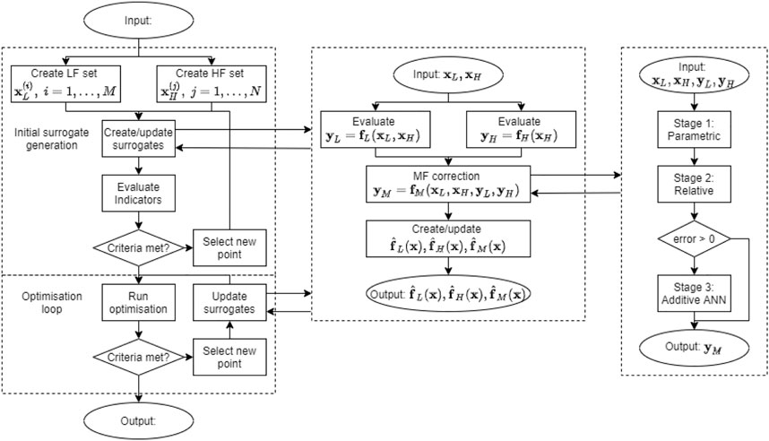
FIGURE 1. The complete integrated MF model management framework. The left-most section represents the outer-loop, including an initial pre-processing step where surrogates are adaptively constructed to meet an acceptable accuracy criteria, and the optimisation loop, where surrogates are iteravely updated as the optimisation process progresses. The middle section represents the MF surrogate generation subroutine, where the create/update action is itself a generic subroutine that accepts only lists of correlated input/output data. Finally, the right-most section represents the MF correction procedure, where in this case the 3-stage approach is implemented. The framework is designed to be modular such that alternative surrogate generation techniques and MF correction methods may be easily substituted.

An advantage of this arrangement is the flexibility allowed during problem formulation. For example, with generalised surrogate generation and correction subroutines, any number of alternative/competing models may be specified for a particular subsystem. Models themselves may have non-equal (or overlapping) input domains, and may be time-phase specific or invariant. Sample points at which models are to be initially evaluated may be supplied, or autonomously selected during the presented surrogate generation procedure. Additionally, existing data may be supplied to augment the model generation process as sets of corresponding input/output arrays. The framework itself is designed to be modular where appropriate, such that alternative surrogate generation techniques and MF correction methods may be easily substituted.

4 Modelling

The proposed model correction and management framework is applied to a series of test cases involving a parameterised Unmanned Space Vehicle (USV). USVs, such as the Boeing X-37B Orbital Test Vehicle (OTV), have been used to return experiments from Low Earth Orbit (LEO) and are often considered as a test bed for the development of future re-usable launchers, with particular emphasis on the key technologies enabling atmospheric re-entry. The USV examined in this study is based on an idealised unpowered waverider (Starkey and Lewis, 2000; Minisci and Vasile, 2013), with the goal of defining the technical specifications for a small, relatively inexpensive technological demonstrator vehicle. Of particular interest is the range of geometric configurations (and corresponding re-entry trajectories) enabling the return of certain types of payload (e.g., delicate or time sensitive) owing to the management of aerodynamic and/or thermal loads. The practicality of such a vehicle is thus inherently dependant on the interaction between geometric configuration and aerodynamic/aerothermal subsystems. Simulating the latter to facilitate numerical design optimisation is traditionally more heavily limited by available computational resource. This problem, therefore, is well suited for examining via a MF approach. This section thus details the modelling strategies employed to represent the vehicle geometry and aerodynamics, the latter via two alternative, competing levels of simulation fidelity.

4.1 Geometry parameterisation

A waverider may be parameterised according to the 2D power law equations presented by Starkey and Lewis (2000). The curvatures of the planform p and the upper surface u are given by:

$y_p=A{x}^n(23)$

$y_u=B{\left(z_u\right)}^n\to z_u={\left(\frac{y_u}{B}\right)}^{\frac{1}{n}}(24)$

where the exponent n ∈ [0, 1] and the positive scaling coefficients A and B are given by:

$A=w/2L^n(25)$

$B=A/{\tan }^n\left(\beta \right)(26)$

where L and w are the vehicle length and width respectively and β is the shock angle. The curvature of the lower surface with an attached shock is given by:

$z_l=x\tan \theta +{\left(y/A\right)}^{1/n}\left(\tan \beta -\tan \theta \right)(27)$

where θ is the wedge angle. Vehicle height h and the surface areas of the planform and base sections S_p and S_b are given by:

$h=L\tan \beta (28)$

$S_p=wL/\left(n+1\right)(29)$

$S_b=S_p\tan \theta (30)$

The geometric design vector d is defined according to the following variable bounds (Minisci and Vasile, 2013); vehicle length L ∈ [2.9, 4.2]m, width w ∈ [1, 2]m, exponent n ∈ [0.2, 0.7], wedge angle θ_w ∈ [7, 11] deg and leading-edge radius r_N ∈ [0.04, 0.06]m. The shock angle β is held fixed at 12 deg. By parameterising in this manner, small variations in d can correspond to significant change in the resulting geometry (Starkey and Lewis, 2000). Three examples, representing the maximum, mean and minimum values of d, are shown in Figure 2.

FIGURE 2

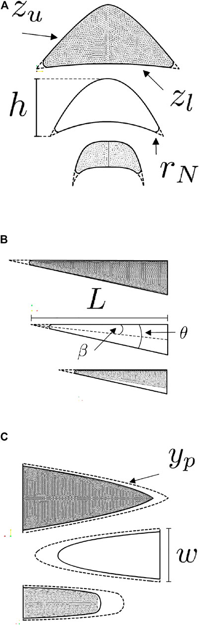
FIGURE 2. Example geometric configurations of a waverider-based USV defined by Eqs 23–30 (Starkey and Lewis, 2000). Orthogonal cross sections are shown aligning with the vehicle’s (A) longitudinal x-axis, (B) lateral y-axis and (C) vertical Z-axis. The three examples included in each subfigure represent the lower, middle and upper values of the vehicle design vector d(L, w, n, θ, r_N).

4.2 Aerodynamics

Two distinct levels of fidelity are considered for the evaluation of the aerodynamic forces acting on the vehicle during re-entry. Each is referred to respectively as “high” and “low” fidelity in primarily a relative sense, in that there exists a significant disparity across both numerical complexity and computational cost between the two. Given this study is more concerned with the inherent disagreement between alternative models rather than their absolute accuracy, extended validation was considered outwith the scope of this work.

4.2.1 Low-fidelity aerodynamics

LF aerodynamics are computed using the Free Open Source Tool for Re-Entry of Asteroids and Debris (FOSTRAD) under development at the University of Strathclyde (Mehta et al., 2015; Falchi et al., 2017b). FOSTRAD discretises solid geometry into surface meshes of triangular elements (panels), to which Local-Surface-Inclination (LSI) based methods are applied. Modified Newtonian Theory and the Schaaf and Chambre analytic model are used to approximate continuum and free-molecular aerodynamic coefficients respectively (Mehta et al., 2015; Falchi et al., 2017a). Transitional regime aerodynamics, defined in Mehta et al. (2015) as 10^–4 < Kn < 100, are approximated using a sigmoid (base 10) bridging function.

4.2.2 High-fidelity aerodynamics

HF aerodynamics are computed using the Stanford University Unstructured Code (SU2) (Palacios et al., 2013). The 3-dimensional RANS equations are employed with a standard SST turbulence model and a finite volume method (FVM) discretisation. The JST scheme is used in conjunction with a second-order scalar upwind discretisation and Venkatakrishnan’s limiter to model convective fluxes. The gradients of the spatial flow variables, required to evaluate viscous fluxes, are calculated using the Green-Gauss method with a CFL number of 1. The linear system is solved using the GMRES method with an error tolerance of 10^–10 and the steady state solution is achieved using the Euler implicit method for time integration. A Cauchy convergence criteria is applied to the Drag function after iteration 10. Convergence is defined as the reduction of the residuals by five orders of magnitude with respect to their initial values, within a maximum number of iterations fixed at 5,000.

4.2.3 Correlation

Table 1 summarises the general numerical correlation between both models, where the coefficients of lift and drag, C_L and C_D, of the vehicle defined by design vector d(L, w, n, θ, r_N) (Section 4.1) are estimated for the operational range defined by Mach number Ma and angle of attack α:

$\begin{array}{l}\hfill 2\le Ma\le 30\\ \hfill 0^{\text{o}}\le \alpha \le 20^{\text{o}}\end{array}(31)$

Of particular note, the values of Pearson’s correlation coefficient r² is significantly higher relative to R². This suggests the two models share similar functional form but are more significantly displaced in output space. This is in line with expectation, as despite differing levels of simulation complexity, both aim to represent the same physical process and thus an appreciable level of similarity would be expected.

TABLE 1

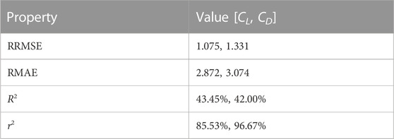
TABLE 1. Numerical accuracy of the low-fidelity (LF) model relative to the high-fidelity (HF) counterpart.

An example of this can be seen in Figure 4, which shows the response surface of the coefficients of lift and drag, C_L and C_D, for the vehicle configuration: L = 3.55m, w = 1.5m, n = 0.45, θ = 9deg and r_N = 0.05m for the operational range given by Eq. 31. In this case, the LFM can be seen to generally over-predict the aerodynamic response, particularly at higher angles of attack. Furthermore, as the LFM includes no specific flow modelling, the functional form (predominantly of C_L) as Mach number increases is notably simpler than that of the HFM. Regardless, the general agreement in form is seen to be quite good, thus conforming to the overall metrics presented in Table 1.

FIGURE 3

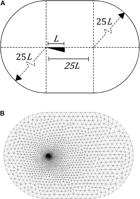
FIGURE 3. An example of the far-field volumetric mesh used for CFD (high-fidelity) simulation, where (A) gives the dimensions relative to vehicle length L (Leifsson et al., 2016) and (B) shows the resulting unstructured mesh, concentrated around the vehicle body surface.

FIGURE 4

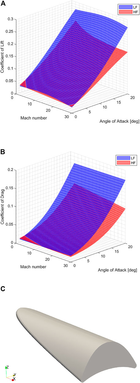
FIGURE 4. Correlation between the coefficients of (A) lift C_L and (B) drag C_D, for (C) the vehicle defined by d(L, w, n, θ, r_N) = [3.55, 1.5, 0.45, 9, 0.05] relative to Mach number Ma and Angle of Attack α.

4.3 2D/3D geometry meshing

The open source meshing tool GMSH (v4.6.0) (Geuzaine and Remacle, 2009) incorporating the OpenCascade geometry kernel is selected for mesh generation. Eqs 23, 24, 27 are used to define the base section and leading edge profile according to the user input vector d. A solid surface (.stl) mesh may then be generated and exported.

To produce a volume mesh suitable for CFD analyses, a half-cylindrical far-field with semi-spherical input/output caps is created around the surface mesh, with the y-symmetry plane bisecting the vehicle geometry along the longitudinal axis, see Figure 3. A single volume mesh is thus created via Boolean subtraction. A simplified boundary mesh definition is incorporated by specifying a vehicle-centered bounding box with internal and external mesh element sizes of 0.025 m, and 10 m respectively, with a transition gradient layer of thickness t = 20m. The vehicle surface mesh is comprised of between 3,500 and 8,000 vertices and between 7,500 and 17000 triangular elements. Likewise, the CFD volume mesh of between 60,000 and 200,000 nodes and 400,000 and 1,400,000 elements. Input, output, far-field and vehicle surfaces are labelled accordingly. The complete volume mesh is exported in the native SU2 format.

5 Multi-fidelity data correction

Parsonage and Maddock (2020) originally presented an isolated test of the proposed response correction functions for a series of fixed geometric designs as well as the complete input domain. This section presents a similar demonstration, though extends the range of HF sampling and focuses on more comparative continuous metrics, including consideration of the variance exhibited by each approach. The coefficients of lift and drag, C_L and C_D, for the vehicle defined by design vector d(L, w, n, θ, r_N) (Section 4.1) are predicted for the operational range defined by Mach number 2 ≤ Ma ≤ 30 and angle of attack 0^o ≤ α ≤ 20^o.

Sample sets of M LF points and N HF points are selected according to Section 3.1, where M = 30d_in (given that the cost of the LF model is relatively low) and N is increased in regular increments from 2 to 40. All samples sets are generated via LHS. For each value of N, the corrected predictions of C_L and C_D are evaluated against an independent testing set of M HF responses. Several variants are considered, where the corrective stages—Parametric (P), Relative (R) and Additive (A)—are applied individually and in sequential combinations. Figure 5; Figure 6 show the values of Relative Maximum Absolute Error (RMAE), Relative Root Mean Square Error (RRMSE) and R² across all values of N for both responses, averaged over 100 separate analyses. Included for reference are the corresponding values of the LF model, and of a simple surrogate model trained only on the set of N HF responses available at the current iteration. This high-fidelity surrogate (HFS) thus represents the baseline above which the multi-fidelity surrogate must perform.

FIGURE 5

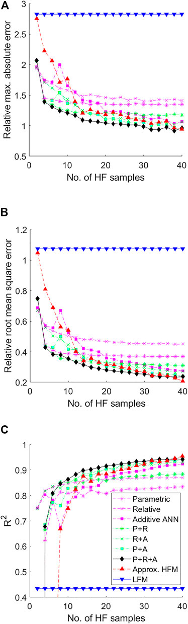
FIGURE 5. Performance metrics of the Parametric (P), Relative (R) and Additive (A) corrective stages applied individually and in sequential combinations for the USV Coefficient of Lift C_L relative to the number of HF evaluations, where (A) is the Relative Max. Absolute Error (RMAE) (B) is the Relative Root Mean Square Error (RRMSE) and (C) is the Coefficient of Determination R². Included for reference are the error values of the LF model, and a SF surrogate trained only on the available HF samples at each iteration.

FIGURE 6

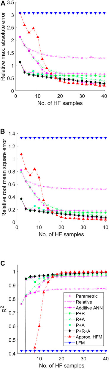
FIGURE 6. Performance metrics of the Parametric (P), Relative (R) and Additive (A) corrective stages applied individually and in sequential combinations for the USV Coefficient of Drag C_D relative to the number of HF evaluations, where (A) is the Relative Max. Absolute Error (RMAE) (B) is the Relative Root Mean Square Error (RRMSE) and (C) is the Coefficient of Determination R². Included for reference are the error values of the LF model, and a SF surrogate trained only on the available HF samples at each iteration.

Considering the responses of both C_D and C_L, a clear hierarchy can be observed between method variants. Single stage methods (P, R and A) exhibit significant limitations in attainable correction quality. The P-stage, for example, is limited by the simplistic nature of the defining parametric operation, and thus while initially offering a strong correction (due to the relatively high model correlation), the effectiveness of successive samples exponentially decreases. In a similar manner, the R-stage is limited by the complexity of the LF model. Given that the LF model by definition can only approximate the true function, even if represented in sufficient resolution it may be expected that the R-stage will result in a comparable limit in quality. Only the A-stage aims to fully eliminate sample point discrepancy in a non-destructive manner. It is reasonable to assume then that correction quality will increase proportional to N, which indeed matches the observed behaviour. However, the converse is naturally seen to be true at lower values of N. Applying stages instead in selected sequential combination (PR, RA, and PA) can be seen to alleviate some of these limitations. For example, preconditioning with the P-stage both improves the converged value of the R-stage and the correction quality/stability for the A-stage at lower values of N. In a similar manner, the RA method both reduces correction instability of the A-stage and the premature convergence of the R-stage. Of note here is that unlike the others, the R-stage does not explicitly aim to reduce sample point discrepancy, and thus is effective as a pre-conditioner to the A-stage. Furthermore, the sequential combination of the P-stage and A-stage is perhaps inefficient, as both are driven by sample point discrepancy. Thus in any combination, the elimination of sample point error renders the other obsolete, largely undesirable when the true response is not yet fully represented. The most appropriate sequence thus includes all three stages, arranged PRA, which can indeed be seen to offer the strongest correction quality for both cases.

The approximate HFS offers the poorest prediction at lower values of N. However, conforming to the conjecture that a suitably trained neural network may represent any non-linear function given sufficient training data (Rumelhart et al., 1994), it can be seen that for each response there exists a value of N after which the HFS is superior. This behaviour is in line with expectation. The MF model by definition always incorporates some less accurate, lower-fidelity data, therefore ultimately cannot reach the same level of accuracy as a pure HF model assuming the latter has sufficient samples and that LF data is not being actively discarded³. This “critical point”, can be seen in this case to be around 38 and 18 samples for C_L and C_D respectively. The significant difference between responses is perhaps surprising given the similar level of correlation between models (see Section 4.2.3). Regardless, the critical point is likely dependant on factors such as problem dimensionality, model correlation and the sampling strategy employed. Concerning the latter, an adaptive sampling strategy that refines the MF approximation by exploiting areas of high predicted improvement and/or maximum discrepancy to improve local accuracy may further increase the attainable prediction quality relative to the overall number of samples. Thus the decline in cost advantage relative to pure HF meta-modelling may be tempered.

The variance in corrective quality was additionally examined as a further extension to the work presented in Parsonage and Maddock (2020). Trained neural networks are highly sensitive to the initial weights, biases and available training data (of a generally low quantity for pure HF modelling). Thus it may be expected that in addition to an exponentially poorer prediction mean at lower values of N, similar behaviour will be observed for prediction variance. This can be seen in Figure 7; Figure 8, which shows the variance in RRMSE observed for each correction stage configuration for C_L and C_D respectively. Indeed, increased variance is observed for each method utilising a neural network (i.e., non-deterministic) stage. Whilst the collaborative effects of each method on prediction quality variance seem to follow the same general behaviour as previously discussed. Of particular interest is that even after the critical point has been reached, there still exists notable variation in the prediction quality of the HFS, likely due to the combination of limited available samples and a lack of any deterministic pre-processing stage(s).

FIGURE 7

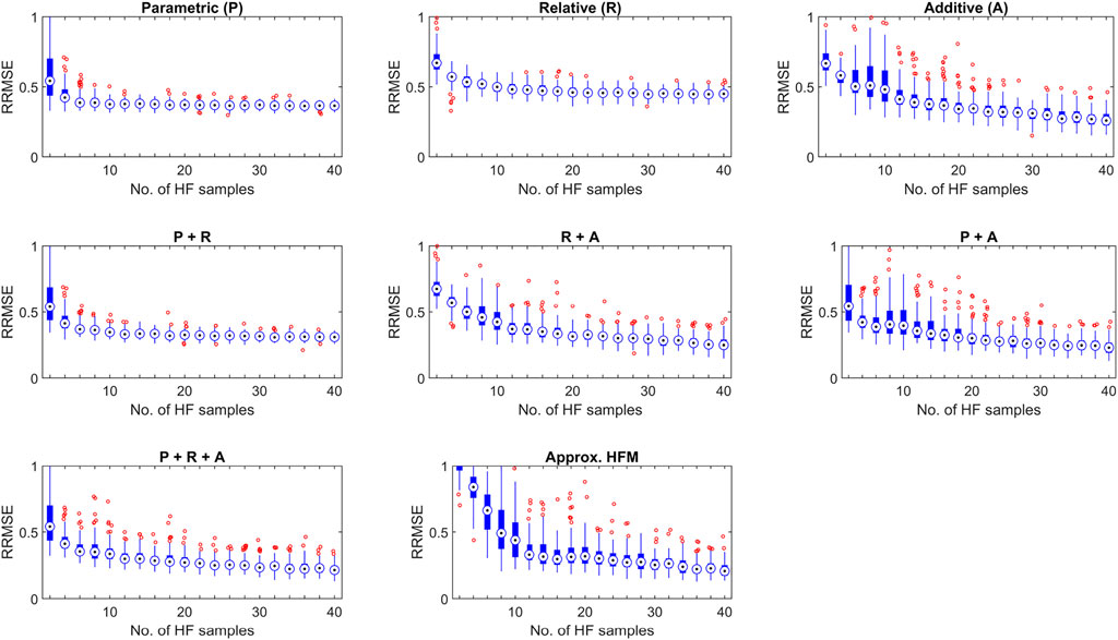
FIGURE 7. Variance in Relative Root Mean Square Error (RRMSE) of the Parametric (P), Relative (R) and Additive (A) corrective stages applied individually and in sequential combinations for the USV Coefficient of Drag C_L relative to the number of HF evaluations. Included for reference is the corresponding performance of the SF surrogate trained only on the available HF samples at each iteration.

FIGURE 8

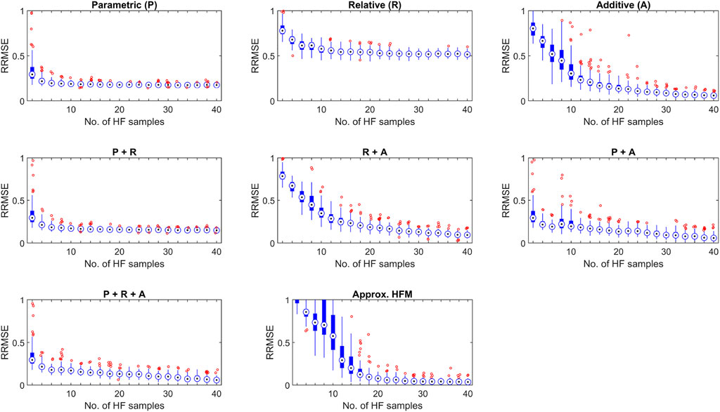
FIGURE 8. Variance in Relative Root Mean Square Error (RRMSE) of the Parametric (P), Relative (R) and Additive (A) corrective stages applied individually and in sequential combinations for the USV Coefficient of Drag C_D relative to the number of HF evaluations. Included for reference is the corresponding performance of the SF surrogate trained only on the available HF samples at each iteration.

6 Optimisation

An application of the proposed framework is demonstrated via a static/dynamic parameter optimisation of the vehicle described in Section 4. This section briefly describes the system dependant processes, problem formulation and settings for the numerical solver.

6.1 System models

The following system models are incorporated into the optimisation problem formulation, in addition to the geometric and aerodynamic model definitions given in Section 4.

6.1.1 Environment

The Earth is modelled as an oblate spheroid based on the WSG-84 model. The gravitational field is modelled using fourth order spherical harmonics (accounting for J2, J3 and J4 terms) for accelerations in the radial g_r and transverse g_t directions. Atmospheric conditions (temperature T_atm, pressure P_atm, density ρ_atm and speed of sound c) are modelled using the Standard US76 global static atmospheric model.

6.1.2 Configuration

Geometric characteristics of the vehicle are taken as presented in Section 4. The total mass of the vehicle is comprised of the structural mass m_structure, the mass of the thermal protection system m_TPS and the mass of the payload (e.g., avionics and power systems) m_payload:

$m_{\mathit{total}}=m_{\mathit{structure}}+m_{\mathit{TPS}}+m_{\mathit{payload}}(32)$

The structural mass is given by:

$m_{\mathit{structure}}={\rho }_{\mathit{body}}\left(2S_p+S_b\right)\ast t_{\mathit{shell}}(33)$

assuming a titanium frame of density ρ_body = 4400 kg/m³ and shell thickness t_shell of 5 mm. The mass of the TPS, chosen as 3 mm thick Zirconium Diboride, ρ_TPS = 6000 kg/m³, is taken as:

$m_{\mathit{TPS}}=m_{\mathit{nose}}+m_{\mathit{skin}}(34)$

where the mass of the nose m_nose is:

$m_{\mathit{nose}}={\rho }_{\mathit{TPS}}{V}_{\mathit{nose}}(35)$

and the mass of the TPS skin covering the remainder of the vehicle m_skin:

$m_{\mathit{skin}}={\rho }_{\mathit{TPS}}{S}_{\mathit{TPS}}{t}_{\mathit{TPS}}(36)$

where S_TPS is the surface area of the vehicle excluding the nose section, approximated by:

$S_{\mathit{TPS}}=2S_p+S_b-2S_n(37)$

The payload mass m_payload is assumed 40% of the structural mass:

$m_{\mathit{payload}}=0.4m_{\mathit{structure}}(38)$

The vehicle “nose” section length is defined as 0.1L, with a corresponding volume V_n approximated as:

$V_n=\frac{w_n{L}_n^2\tan \theta }{\left(n+1\right)\left(n+2\right)}(39)$

6.1.3 Aerodynamics

Aerodynamic evaluation may be performed using either LF or HF solvers introduced in Section 4.

6.1.4 Aerothermodynamics

For this simplified analysis it is assumed that the peak heat flux exists at the vehicle nose section (Minisci et al., 2011). The convective heat flux is evaluated using the analytical formula as given by Anderson Jr (2006):

${\dot{q}}_{\mathit{conv}}=K_e\sqrt{\frac{{\rho }_{\infty }}{r_N}}{v}^3(40)$

where Ke = 1.742e⁻⁴ for ${\dot{q}}_{\mathit{conv}}[W/m^2]$.

6.1.5 Dynamics

A 3-DOF dynamic model expressed in an Earth-Centred-Earth-Fixed (ECEF) reference frame is used. The state vector is comprised of the spherical coordinates for position r = [r, λ, θ] and velocity v = [ν, γ, χ], where r is the radial distance, (λ, θ) are the latitude and longitude, ν is the magnitude of the relative velocity vector directed by the flight path angle γ and the flight heading angle χ.

$\dot{r}=\nu \sin \gamma (41)$

$\dot{\lambda }=\frac{\nu \cos \gamma \cos \chi }{r}(42)$

$\dot{\theta }=\frac{\nu \cos \gamma \sin \chi }{r\cos \lambda }(43)$

$\begin{array}{ll}\hfill \dot{\nu }& =\frac{F_T\left(\tau \right)\cos \alpha -D\left(\alpha \right)}{m}-g_r\sin \gamma +g_t\cos \gamma \cos \chi \hfill \\ \hfill & +{\omega }_E^{2}r\cos \lambda \left(\sin \gamma \cos \lambda -\cos \gamma \cos \chi \sin \lambda \right)\hfill \end{array}(44)$

$\begin{array}{ll}\hfill \dot{\gamma }& =\frac{1}{\nu }\left(\frac{F_T\left(\tau \right)\sin \alpha +L\left(\alpha \right)}{m}\cos \beta -g_r\cos \gamma -g_t\sin \gamma \cos \chi \right)+\frac{\nu }{r}\cos \gamma \hfill \\ \hfill & +\frac{{\omega }_E^{2}r}{\nu }\cos \lambda \left(\sin \gamma \cos \chi \sin \lambda +\cos \gamma \cos \lambda \right)+2{\omega }_E\sin \chi \cos \lambda \hfill \end{array}(45)$

$\begin{array}{ll}\hfill \dot{\chi }& =\frac{1}{\nu \cos \gamma }\left(\frac{F_T\left(\tau \right)\sin \alpha +L\left(\alpha \right)}{m}\sin \beta -g_t\sin \chi \right)+\frac{v}{r}\cos \gamma \sin \chi \tan \lambda \hfill \\ \hfill & +{\omega }_E^{2}r\frac{\sin \chi \sin \lambda \cos \lambda }{\nu \cos \gamma }+2{\omega }_E\left(\sin \lambda -\tan \gamma \cos \chi \cos \lambda \right)\hfill \end{array}(46)$

$\dot{\alpha }=\frac{\partial \alpha }{\partial t}(47)$

In this case, the thrust force F_T = 0 and angle τ = 0 deg. No out-of-plane movement is considered, thus bank angle β = 0 deg.

6.2 Problem formulation

A generic optimal control problem may be formulated as follows (Ricciardi et al., 2019):

$\begin{array}{c}\hfill \underset{u\in U,b\in B}{\min }\mathbf{J}\\ \hfill s.t.\dot{\mathbf{x}}=\mathbf{F}\left(\mathbf{x},\mathbf{u},\mathbf{b},t\right)\\ \hfill \mathbf{g}\left(\mathbf{x},\mathbf{u},\mathbf{b},t\right)\ge 0\\ \hfill \mathit{\psi }\left({\mathbf{x}}_0,{\mathbf{x}}_f,t_0,t_f,\mathbf{b}\right)\ge 0\\ \hfill t\in \left[t_0,t_f\right]\end{array}(48)$

where $\mathbf{J}={[J_1,\dots ,J_m]}^T$ is a vector of objectives J_i each a function of the state vector $\mathbf{x}:[t_0,t_f]\to {\mathbb{R}}^n$, control variables $\mathbf{u}\in L^{\infty }\left(\right.U\subseteq {\mathbb{R}}^{n_u}$, static parameters $\mathbf{b}\in \mathbf{B}\subseteq {\mathbb{R}}^{n_b}$ and time t. The functions x(t) belong to the Sobolev space W^1,∞ while the other objective functions are $J_i:{\mathbb{R}}^{3n+2}\times {\mathbb{R}}^{n_u}\times {\mathbb{R}}^{n_b}\to \mathbb{R}$. The objective vector is subject to a set of dynamic constraints with $\mathbf{F}:{\mathbb{R}}^n\times {\mathbb{R}}^{n_u}\times {\mathbb{R}}^{n_b}\times [t_0,t_f]\to {\mathbb{R}}^n$, algebraic constraints $\mathbf{g}:{\mathbb{R}}^n\times {\mathbb{R}}^{n_u}\times {\mathbb{R}}^{n_b}\times [t_0,t_f]\to {\mathbb{R}}^{n_g}$ and boundary conditions $\mathit{\psi }:{\mathbb{R}}^{2n+2}\times {\mathbb{R}}^{n_b}\to {\mathbb{R}}^{\psi }$. This work considers Mayer’s type of optimal control problem, each objective function therefore being represented by a scalar function of the boundary conditions, boundary times and static parameters:

$J_i=\varphi \left({\mathbf{x}}_0,{\mathbf{x}}_f,t_0,t_f,\mathbf{b}\right)(49)$

The problem is solved using an in-house, open source multi-objective optimal control solver, MODHOC (Ricciardi and Vasile, 2018), integrated with the presented MF management framework. MODHOC transcribes the optimisation problem into a non-linear programming (NLP) problem via the Direct Finite Elements in Time (DFET) method (Vasile, 2010).

Static design parameters and the open-loop control of the vehicle are optimised according to the parameters given in Table 2. Three problem objectives are considered, each requiring a distinct degree of aerodynamic performance; the minimisation of peak convective heat flux experienced during re-entry ${\dot{q}}_{\mathit{conv}}$, the minimisation of total time required to reach terminal conditions t_f, and the minimisation of the peak dynamic pressure q. Each problem is subject to path constraints on convective heat flux ${\dot{q}}_{\mathit{conv}}\le {({\dot{q}}_{\mathit{conv}})}_{\max }$, dynamic pressure q ≤ q_max and axial acceleration [a_x, a_z] ≤ a_max. The computational resource required to converge in each case is examined using both the MF model management framework and an equivalent single-fidelity (SF) approach.

TABLE 2

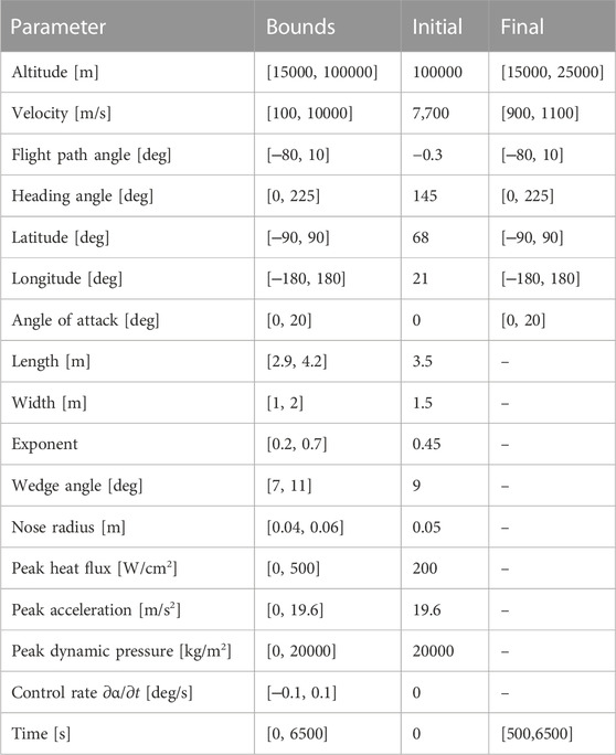
TABLE 2. Optimisation parameters.

6.3 Numerical settings

Each problem is considered as a single time phase, with boundary conditions given in Table 2 and discretised into six finite elements. States and controls are represented by element specific ninth order Bernstein polynomials, giving 496 total optimisation parameters (60 control, 427 state and nine static). Single objective optimisation was completed using the gradient based solver fmincon with a SQP algorithm. Limits of 1000 objective function evaluations and 100 outer level iterations were imposed for each run. The maximum function, constraint violation and step tolerances are set at 1e-9, 1e-12 and 1e-12 respectively.

7 Results

7.1 High/low fidelity solutions

As a reference, the problem was first solved for each objective using pre-constructed well-fit⁴ surrogate approximations of the HF and LF aerodynamic models. The optimal designs for each single-objective problem, relative to fidelity level, are given in Table 3. Figures 9, 10 show the geometry and state trajectories for each problem solved using the HF aerodynamic model.

TABLE 3

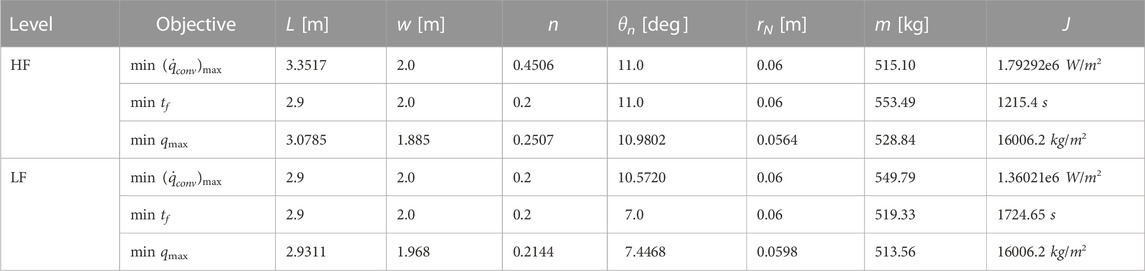
TABLE 3. High/Low fidelity solutions.

FIGURE 9

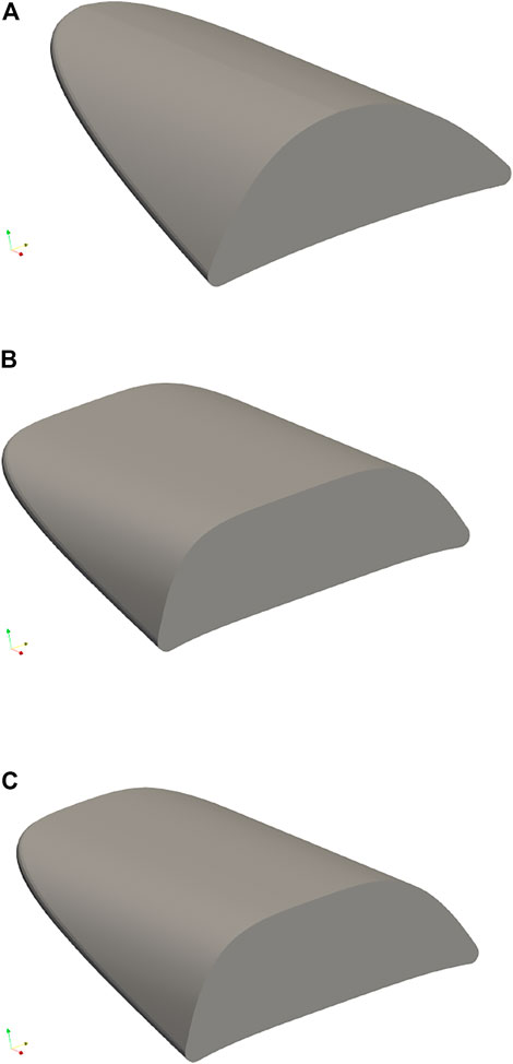
FIGURE 9. Geometric design solutions obtained using only HF aerodynamic model. The single objective in each case is the minimisation of (A) peak convective heat flux at the vehicle nose ${({\dot{q}}_{\mathit{conv}})}_{\max }$ (B) the total time taken to reach terminal conditions t_f and (C) the peak dynamic pressure experience during re-entry q_max.

FIGURE 10

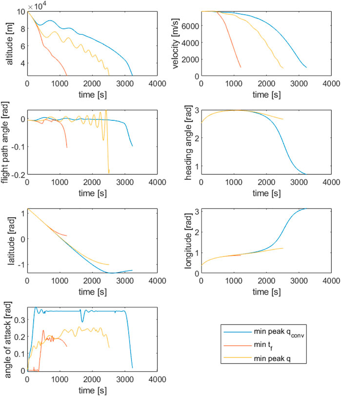
FIGURE 10. Dynamic state solutions obtained using only the HF aerodynamic model. The objective functions considered are the minimisation of peak convective heat flux at the vehicle nose ${({\dot{q}}_{\mathit{conv}})}_{\max }$, the total time taken to reach terminal conditions t_f and the peak dynamic pressure experience during re-entry q_max.

As a general theme, the optimiser favours shorter, wider vehicles with larger values of leading edge radius (the latter likely due to the significant effect on peak heating). The primary difference between solutions is then the resulting mass of each vehicle, driven by the shape exponent value n. This is possibly a result of an attempt to maximise effective lifting surface whilst incurring minimal mass penalty. The effects may be seen in the HF trajectory solutions, where the lighter vehicles utilise greater proportions of high altitude gliding to dissipate excess energy, ultimately allowing a gentler descent through the denser regions of the atmosphere. In contrast, the heavier solution (minimum t_f) exhibits a rapid descent through the upper regions of the atmosphere before utilising larger drag forces to decelerate as air density increases.

Similar contrasts can be seen in the angle of attack profiles. The minimum t_f solution maintains close to 0deg during the initial descent, before flaring to 10deg at around 60 km in order to decelerate within the aerodynamic loading constraints. The minimum ${({\dot{q}}_{\mathit{conv}})}_{\max }$ solution displays an almost constant saturation at the maximum allowable value of 20deg, suggesting that this bound is imposing a significant constraint on the available solution. While at this incidence, the stagnation point for convective heat transfer is likely located at the vehicle nose (Minisci et al., 2011), allowing the vehicle to reach more realistic values (40–45deg) would possibly shift this point further down the lower surface, and thus require more sophisticated aero-thermodynamic modelling. In the case where aerodynamic heating is less of a constraint, the optimiser appears to correlate a smaller leading edge radius with improved hypersonic aerodynamic performance.

7.2 Multi-fidelity solutions

The proposed framework is used to solve each single-objective problem. Each analysis is terminated upon reaching a designated maximum number of allowable HF evaluations, N_max = 40. Figures 11, 12 show the convergence of each problem solution relative to the number of samples, where the latter utilises only a SF surrogate. In this case, the model is generated using direct non-adaptive sample sets of size N. The solutions obtained when using only the LF and HF models respectively are included for reference.

FIGURE 11

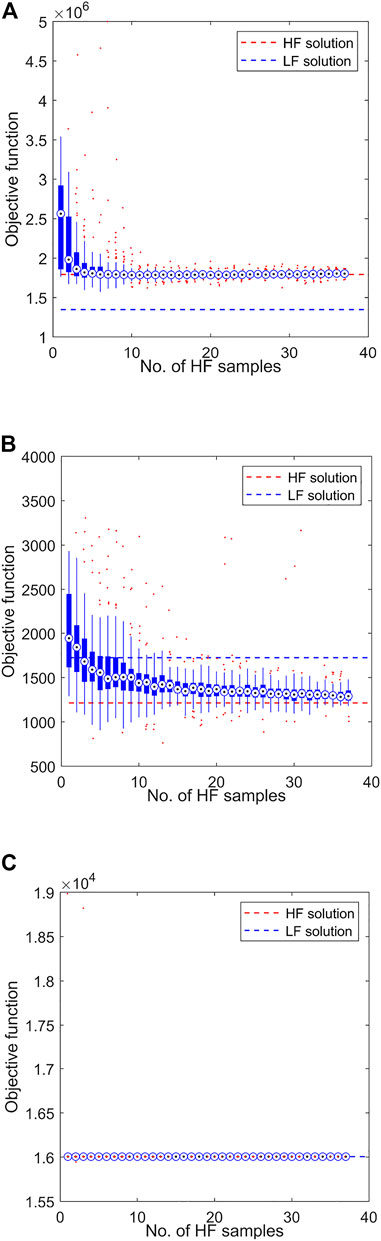
FIGURE 11. Objective function convergence when using the MF surrogate management framework, where the objective functions considered are the minimisation of (A) peak convective heat flux ${({\dot{q}}_{\mathit{conv}})}_{\max }$, (B) total time taken to reach terminal conditions t_f and (C) the peak dynamic pressure experienced during re-entry q_max.

FIGURE 12

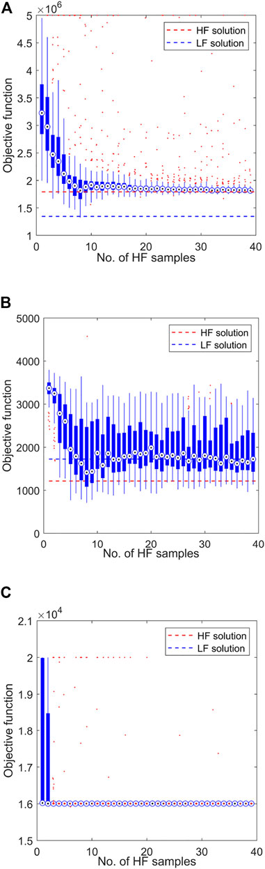
FIGURE 12. Objective function convergence when using a SF aerodynamic surrogate trained only on the available HF samples. The objective functions considered are the minimisation of (A) peak convective heat flux ${({\dot{q}}_{\mathit{conv}})}_{\max }$, (B) total time taken to reach terminal conditions t_f and (C) the peak dynamic pressure experienced during re-entry q_max.

In each case, the MF optimisation demonstrates convergence to the HF optimum. The SF method achieves reasonable convergence for the min peak ${\dot{q}}_{\mathit{conv}}$ and min q_max cases, though fails to show similar performance for the min t_f case. While it is possible that outwith the limited number of HF model evaluations considered the SF surrogate would indeed allow convergence to the “true” solution, it can non-etheless be seen that the model management framework does so within a reduced computational cost. Furthermore, the MF solution is seen to offer a reduced measure of uncertainty compared with the SF alternative. Disproportionate variation relative to the expected surrogate accuracy (see Section 5) is likely the result of a cascading effect driven by the inherent randomisation within the model training procedure i.e., slight differences in approximation encourage the optimiser to converge on a significantly altered solution. Intuitively, this issue would appear to be more prevalent for the surrogates built on limited datasets (and thus altogether less reliably representative of global trends), as is the case for the single-fidelty surrogate. The MF surrogate however, whilst incorporating the same amount of HF data, is trained using a comparatively larger dataset of unique points given the inclusion of supplemental LF data during the information correction process. Thus it would be expected that the MF surrogate would exhibit proportionally less variation between successive updates. A consequential implication is that although a given iteration above such a “critical value” of N (see Section 5) may generate a SF surrogate of higher measurable accuracy than the MF counterpart, it is use within an iterative refinement scheme may still yet be misleading given the remaining probabilistic uncertainty in current and future iterations.

Less definite convergence is seen when examining the progression of the vehicle design vector d(L, w, n, θ, r_N). For example, Figure 13 shows the average component values of d(L, w, n, θ, r_N) relative to the number of HF samples N for both the model management approach and the SF approach. It can be seen that the vehicle width w, wedge angle θ and leading edge radius r_N design parameters tend to reasonably adherence to the HF solution within the prescribed budget, with length L and exponent n values showing only weak convergence trends at best. Nonetheless, it is observed that in all cases, the model management framework can be said to facilitate convergence upon the “true” solution in less HF evaluations than the equivalent SF approach, if indeed the latter converges at all within the allotted budget.

FIGURE 13

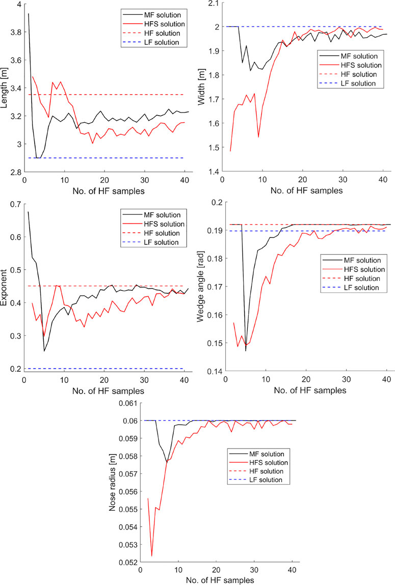
FIGURE 13. Averaged values of vehicle design vector d(l, w, n, θ, r_N) relative to the number of available HF samples during the optimisation process, where the objective function considered is the minimisation of peak convective heat flux ${({\dot{q}}_{\mathit{conv}})}_{\max }$. The black line represents the results obtained using the MF management framework. The red line represents those obtained using only a SF aerodynamic surrogate trained on the available HF samples. Included for reference are the values obtained when solving the prescribed problem using only the LF and HF aerodynamic models respectively.

In all cases however, the probability of variation in each design variable is much higher than observed for the corresponding objective function. Particularly in cases that exhibit a strong objective convergence with respect to N, the disparity across the design vector d suggests that the sensitivity (or lack thereof) of the problem objective function to a particular design variable has a significant impact on the correction procedure. For example, Figure 14 shows the distribution of vehicle exponent n relative to N for both MF and SF approaches. Though the average value tends to converge on the “true” value in less HF samples than the equivalent SF method, at the final iteration there still exists a significant interquartile range, and may indeed still saturate almost to either minimum or maximum bound. This is supported via a closer examination of the sensitivities of the LF and HF models. Table 4 shows the sensitivities of each output with respect to each input for both the LF and HF models. A clear dominance of the angle of attack α on the function responses compared to the remaining input variables is seen, supporting the conjecture that design vector sampling has been largely overshadowed by the predominance of the angle of attack on aerodynamic response. This then raises the question that, despite the cost savings achievable via a sensitivity-biased sampling approach, if the “less important” variables are more relevant to design/mission performance via a different subsystem, there then may exist a functional disconnect within the optimisation process, potentially compromising the obtained results.

FIGURE 14

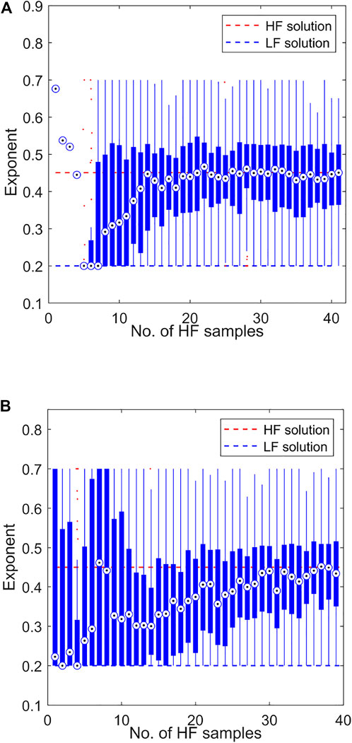
FIGURE 14. Distribution values of the vehicle exponent n relative to the number of HF evaluations when solving for the minimum peak convective heat flux ${({\dot{q}}_{\mathit{conv}})}_{\max }$ using (A) the MF management framework and (B) the equivalent SF surrogate.

TABLE 4

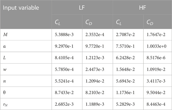
TABLE 4. Sensitivity of each output to each input variable, for both the low-fidelity (LF) and high-fidelity (HF) models.

7.3 K-fold cross validation error

To briefly demonstrate the surrogate quality achieved via the proposed methodology during the optimisation process, Figure 15 shows the K-fold Cross Validation Error (K-CVE) recorded for each MF aerodynamic surrogate, relative to each test case. Of note is that the relative improvement in K-CVE is largely independent of the particular objective function considered.

FIGURE 15

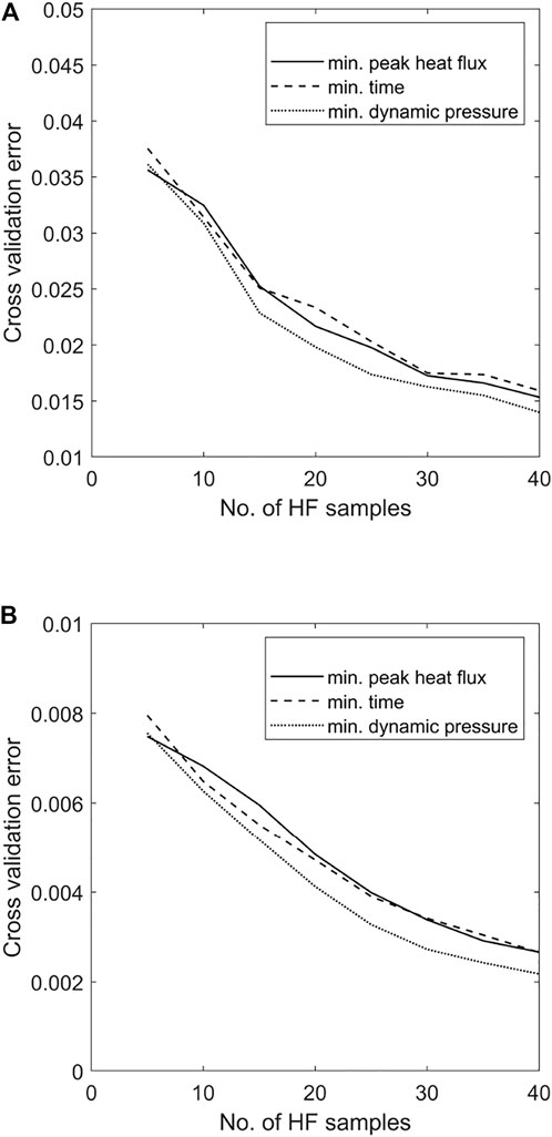
FIGURE 15. K-fold cross validation errors recorded for the MF surrogates of (A) Coefficient of Lift C_L and (B) Coefficient of Drag C_D when solving for each prescribed objective function using the MF model management framework.

8 Cost

With regards to the presented application, the goal was to demonstrate the cost savings offered by the proposed MF approach. This section presents a brief cost report considering the framework as a whole. The presented results were obtained over 100 independent runs using a 2.5 GHz Intel(R) Core(TM) i5-7200 CPU with 8 GB RAM.

The average execution times (with standard deviations included in brackets) recorded for a single run of the aerodynamic solvers FOSTRAD and SU2 were 17.21s (4.96s) and 6165s (4077s) respectively. Geometry generation using GMSH accounted for an additional 12.24s (4.1s) for a 2D surface mesh and 34.43s (11.19s) for a 3D volume mesh. The average run-time of a trained ANN surrogate was found to be 1.0388e-4s (4.7078e-04s).

Table 5 presents the execution times required by each stage of the optimisation process. Included where appropriate are the corresponding values for the SF process using only HF function evaluations. A number of significant disparities can be seen. Firstly, the generation of initial surrogates takes much longer for the MF managed approach due to the iterative initial sampling procedure, terminating only when the surrogates have reached acceptable quality. The SF approach in contrast simply generates surrogates following simple one-shot sampling. Furthermore, this procedure is performed only once during the MF process, wheres the SF results are representative of the time taken each iteration. Secondly, the MF managed procedure is an order of magnitude faster when generating the initial guess to be supplied to the optimiser and subsequently converging on an optimal solution. This is in part due to the higher quality of the MF surrogate models given the extended sampling and training procedures in operation, but also likely given the stability in variation as a result of the proposed correction process, discussed previously in Section 5. Finally, the reported times for SM update are representative of the time taken to adaptively select new sample points for MF correction, and the subsequent update of the current set of surrogates.

TABLE 5

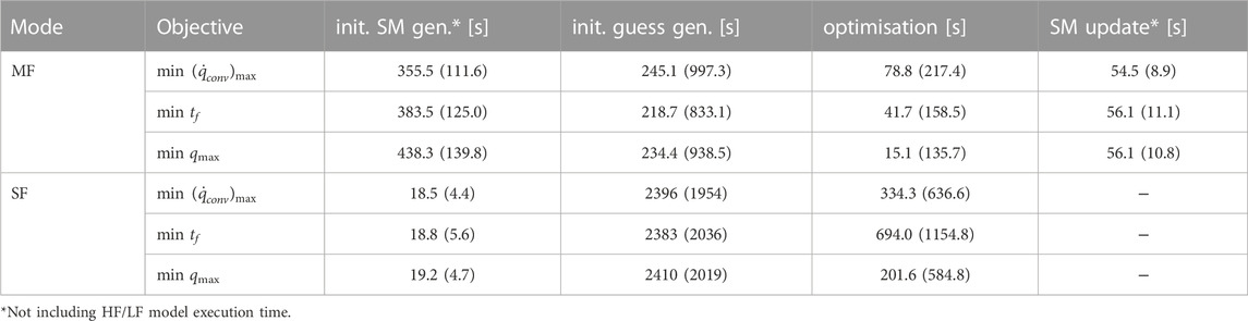
TABLE 5. Average execution times for the primary stages of the multi-fidelity (MF) optimisation process. Included for reference are the corresponding values for the single-fidelity (SF) process. Standard deviations for each are included in brackets.

Considering the complete process, Figure 16 shows the total execution time of the MF management framework and the SF optimisation process for each of the examined test cases. In each case, the MF management framework is seen to facilitate convergence to the HF solution at a increased rate relative to the SF approach.

FIGURE 16

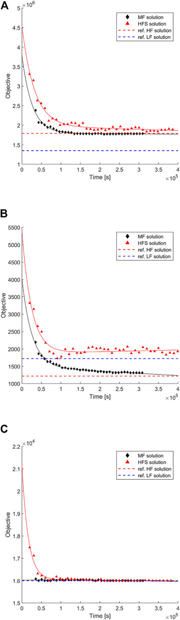
FIGURE 16. Total execution times of the MF management framework and the SF optimisation process for the (A) minimum peak heat flux ${({\dot{q}}_{\mathit{conv}})}_{\max }$, (B) minimum time t_f and (C) minimum dynamic pressure q_max test cases.

9 Conclusion

This paper demonstrates an approach to incorporate increased levels of simulation fidelity into multi-objective design optimisation problem within a minimised cost budget. Alternative aspects of LF data are used to facilitate an information correction process, with configurable alternatives compared in terms of available accuracy and computational cost. It is found that the sequential application of corrective stages allows a greater attainable approximation accuracy relative to a SF equivalent model for a set number of HF samples up to some critical value. The effectiveness of such correction is generally found to be proportional to the ratio N_crit/N_local. An application of this approach is demonstrated via the aerodynamic response prediction of a parametrised waverider subject to a static/dynamic parameter optimisation. Correction quality is found to be consistent across the input domain, though naturally decreasing with dimensionality. Clear convergence to the optimum is observed via the MF management framework for each of the three examined single-objective formulations, in two cases significantly outperforming the equivalent SF solution in terms of number of required HF samples. Convergence of the static design solution is less consistent, likely a result of the sensitivity based adaptive sampling approach, which tends to favour variables exhibiting a larger influence on the surrogate output parameters. A cascading effect due to unstable surrogate quality is observed, in which slight differences in zero- and first-order surrogate approximation results in significantly different problem solutions. This effect is seen to be much more prevalent for surrogates trained on limited datasets, as is primarily the case for the SF equivalent networks.

Fundamentally, a primary disadvantages of this approach may then stem from the attempted generalisation, in that the assumption of no a priori knowledge is perhaps unfounded for most real-world applications. In this case, MF approaches more tailored to the concerned physical process(es) may achieve higher performance. However, the proposed framework and/or methodology may still be incorporated into further early-phase multidisciplinary optimisation processes to aid the rapid validation of design trade-offs and determine interdisciplinary coupling/sensitivities.

Data availability statement

The raw data supporting the conclusions of this article will be made available by the authors, without undue reservation.

Author contributions

The research presented in this paper has been completed by BP as part of his PhD studies, supervised by CM.

Acknowledgments

The results presented in Sections 5, 7 were obtained using the ARCHIE-WeSt High Performance Computer (www.archie-west.ac.uk).

Conflict of interest

The authors declare that the research was conducted in the absence of any commercial or financial relationships that could be construed as a potential conflict of interest.

Publisher’s note

All claims expressed in this article are solely those of the authors and do not necessarily represent those of their affiliated organizations, or those of the publisher, the editors and the reviewers. Any product that may be evaluated in this article, or claim that may be made by its manufacturer, is not guaranteed or endorsed by the publisher.

Footnotes

¹also referred to as variable-fidelity.

²Whilst the random division of input data in Eq. 1 means that the resulting subsets cannot be thus assumed space filling themselves, the variation of subset assignment within the inner-level loop is intended to minimise any resulting bias.

³Which indeed is the premise behind methods such as Trust Region Model Management (Alexandrov et al., 2001).

⁴i.e., using LHS selected sampling sets of size n_s = 30n_input, trained using the procedure described in Section 2 to R² > 99.5.

References

Alexandrov, N., Branch, M. D. O., Larc, N., Dennis, J. E., Michael, R., Icase, L., et al. (1997). A trust region framework for managing the use of approximation models in optimization. Struct. Optim. 15, 16–23. doi:10.1007/BF01197433

CrossRef Full Text | Google Scholar

Alexandrov, N. M., Lewis, R. M., Gumbert, C. R., Green, L. L., and Newman, P. A. (2001). Approximation and model management in aerodynamic optimization with variable-fidelity models. J. Aircr. 38, 1093–1101. doi:10.2514/2.2877

CrossRef Full Text | Google Scholar

Allaire, D., and Willcox, K. (2014). A mathematical and computational framework for multifidelity design and analysis with computer models. Int. J. Uncertain. Quantification 4, 1–20. doi:10.1615/Int.J.UncertaintyQuantification.2013004121

CrossRef Full Text | Google Scholar

Anderson, J. D. (2006). Hypersonic and high-temperature gas dynamics. Reston, VA: American Institute of Aeronautics and Astronautics.

Google Scholar

Bandler, J. W., Biernacki, R. M., Chen, S. H., Grobelny, P. A., and Hemmers, R. H. (1994). Space mapping technique for electromagnetic optimization. IEEE Trans. Microw. Theory Tech. 42, 2536–2544. doi:10.1109/22.339794

CrossRef Full Text | Google Scholar

Beale, M. H., Hagan, M. T., and Demuth, H. B. (2017). Neural network Toolbox ^TMUser’s guide R2017b.

Google Scholar

Booker, A. J., Dennis, J. E., Frank, P. D., Serafini, D. B., Torczon, V., and Trosset, M. W. (1999). A rigorous framework for optimization of expensive functions by surrogates. Struct. Optim. 17, 1–13. doi:10.1007/BF01197708

CrossRef Full Text | Google Scholar

Bryson, D. E., Haimes, R., and Dannenhoffer, J. F. (2019). “Toward the realization of a highly integrated, multidisciplinary, multifidelity design environment,” in AIAA Scitech 2019 Forum, 7-11 January 2019. San Diego, California, 1–15. doi:10.2514/6.2019-2225

CrossRef Full Text | Google Scholar

Christensen, D. E., and Willcox, K. (2012). Multifidelity methods for multidisciplinary design under uncertainty. Ph.D. thesis. Cambridge, MA: Massachusetts Institute of Technology.

Google Scholar

Falchi, A., Minisci, E., Vasile, M., Rastelli, D., and Bellini, N. (2017a). “DSMC-Based correction factor for low-fidelity hypersonic aerodynamics of Re-entering objects and space Debris,” in 7th European Conference of Aeronautics and Aerospace Sciences, Milan, Italy, 10.

Google Scholar

Falchi, A., Vasile, M., Falchi, A., Renato, V., Minisci, E., and Vasile, M. (2017b). “Fostrad: An advanced open source tool for Re-entry analysis,” in 15th Reinventing Space Conference, Glasgow, UK, 1–15.

Google Scholar

Fernandez, G., Park, C., Kim, N. H., and Haftka, R. (2017). Review of multi-fidelity models.

Google Scholar

Fernández-Godino, M. G., Park, C., Kim, N.-H., and Haftka, R. T. (2016). Review of multi-fidelity models.

Google Scholar

Fischer, C. C., Grandhi, R. V., and Beran, P. S. (2018). Bayesian-enhanced low-fidelity correction approach to multifidelity aerospace design. AIAA J. 56, 3295–3306. doi:10.2514/1.J056529

CrossRef Full Text | Google Scholar

Forrester, A. I., and Keane, A. J. (2009). Recent advances in surrogate-based optimization. Prog. Aerosp. Sci. 45, 50–79. doi:10.1016/j.paerosci.2008.11.001

CrossRef Full Text | Google Scholar

Forrester, A. I., Sóbester, A., and Keane, A. J. (2007). Multi-fidelity optimization via surrogate modelling. Proc. R. Soc. A Math. Phys. Eng. Sci. 463, 3251–3269. doi:10.1098/rspa.2007.1900

CrossRef Full Text | Google Scholar

Gano, S. E., Renaud, J. E., and Sanders, B. (2005). Hybrid variable fidelity optimization by using a kriging-based scaling function. AIAA J. 43, 2422–2433. doi:10.2514/1.12466

CrossRef Full Text | Google Scholar

Geuzaine, C., and Remacle, J.-F. (2009). Gmsh: A 3-D finite element mesh generator with built-in pre-and post-processing facilities. Int. J. Numer. Methods Eng. 79, 1309–1331. doi:10.1002/nme.2579

CrossRef Full Text | Google Scholar

Goel, T., Haftka, R. T., Shyy, W., and Queipo, N. V. (2007). Ensemble of surrogates. Struct. Multidiscip. Optim. 33, 199–216. doi:10.1007/s00158-006-0051-9

CrossRef Full Text | Google Scholar

Gramacy, R. B., and Lee, H. K. (2009). Adaptive design and analysis of supercomputer experiments. Technometrics 51, 130–145. doi:10.1198/TECH.2009.0015

CrossRef Full Text | Google Scholar

Guenther, J., Lee, H. K., and Gray, G. A. (2015). Sequential design for achieving estimated accuracy of global sensitivities. Appl. Stoch. Models Bus. Industry 31, 782–800. doi:10.1002/asmb.2091

CrossRef Full Text | Google Scholar

Han, Z. H., Görtz, S., and Hain, R. (2010). “A variable-fidelity modeling method for aero-loads prediction,” in New results in numerical and experimental fluid mechanics VII. Notes on numerical fluid mechanics and multidisciplinary design. Editors A. Dillmann, G. Heller, M. Klaas, H. P. Kreplin, W. Nitsche, and W. Schröder (Berlin, Heidelberg: Springer), Vol. 112, 17–25. doi:10.1007/978-3-642-14243-7_3

CrossRef Full Text | Google Scholar

Han, Z. H., Görtz, S., and Zimmermann, R. (2013). Improving variable-fidelity surrogate modeling via gradient-enhanced kriging and a generalized hybrid bridge function. Aerosp. Sci. Technol. 25, 177–189. doi:10.1016/j.ast.2012.01.006

CrossRef Full Text | Google Scholar

Heath, G. (2020). Mathworks community profile - greg Heath.

Google Scholar

Huang, L., Gao, Z., and Zhang, D. (2013). Research on multi-fidelity aerodynamic optimization methods. Chin. J. Aeronautics 26, 279–286. doi:10.1016/j.cja.2013.02.004

CrossRef Full Text | Google Scholar

Jansen, M. J. (1999). Analysis of variance designs for model output. Comput. Phys. Commun. 117, 35–43. doi:10.1016/S0010-4655(98)00154-4

CrossRef Full Text | Google Scholar

Jones, D. R., Schonlau, M., and Welch, W. J. (1998). Efficient global optimization of expensive black-box functions. J. Glob. Optim. 13, 455–492. doi:10.1023/a:1008306431147

CrossRef Full Text | Google Scholar

Keane, A. J. (2003). Wing optimization using design of experiment, response surface, and data fusion methods. J. Aircr. 40, 741–750. doi:10.2514/2.3153

CrossRef Full Text | Google Scholar

Kennedy, M. C., and O’Hagan, A. (2001). Bayesian calibration of computer models. J. R. Stat. Soc. Ser. B Stat. Methodol. 63, 425–464. doi:10.1111/1467-9868.00294

CrossRef Full Text | Google Scholar

Kim, B., Lee, Y., and Choi, D. H. (2009). Construction of the radial basis function based on a sequential sampling approach using cross-validation. J. Mech. Sci. Technol. 23, 3357–3365. doi:10.1007/s12206-009-1014-z

CrossRef Full Text | Google Scholar

Kolmogorov, A. N. (1957). On the representation of continuous functions of several variables as superpositions of continuous functions of one variable and addition. Dokl. Akad. Nauk. USSR 114, 679–681. doi:10.18411/lj-12-2018-148

CrossRef Full Text | Google Scholar

Koziel, S., Cheng, Q., and Bandler, J. W. (2008). Space mapping. Piscataway, NJ, USA: IEEE Microwave Magazine, 105–122.

CrossRef Full Text | Google Scholar

Koziel, S., and Leifsson, L. (2012). “Knowledge-based airfoil shape optimization using space mapping,” in 30th AIAA applied aerodynamics conference, New Orleans, Louisiana, 25 June 2012 - 28 June 2012, 3016. doi:10.2514/6.2012-3016

CrossRef Full Text | Google Scholar

Koziel, S., and Leifsson, L. (2016). Simulation-driven design by knowledge-based response correction techniques. Cham: Springer. doi:10.1007/978-3-319-30115-0

CrossRef Full Text | Google Scholar

Leifsson, L., Koziel, S., and Tesfahunegn, Y. (2016). Fast multi-objective aerodynamic optimization using space-mapping-corrected multi-fidelity models and kriging interpolation. Cham: Springer, 153. doi:10.1007/978-3-319-27517-8

CrossRef Full Text | Google Scholar

Liu, H., Ong, Y. S., and Cai, J. (2018). A survey of adaptive sampling for global metamodeling in support of simulation-based complex engineering design. Struct. Multidiscip. Optim. 57, 393–416. doi:10.1007/s00158-017-1739-8

CrossRef Full Text | Google Scholar

March, A., and Willcox, K. (2012a). Constrained multifidelity optimization using model calibration. Struct. Multidiscip. Optim. 46, 93–109. doi:10.1007/s00158-011-0749-1

CrossRef Full Text | Google Scholar

March, A., and Willcox, K. (2012b). Provably convergent multifidelity optimization algorithm not requiring high-fidelity derivatives. AIAA J. 50, 1079–1089. doi:10.2514/1.J051125

CrossRef Full Text | Google Scholar

McCulloch, W. S., and Pitts, W. H. (1943). A logical calculus of the ideas immanent in nervous activity. Bull. Math. Biophysics 5, 115–133. doi:10.1007/bf02478259

CrossRef Full Text | Google Scholar

Mehta, P. M., Minisci, E., Vasile, M., Walker, A. C., and Brown, M. (2015). “An open-source hypersonic aerodynamic and aerothermodynamic modeling tool,” in 8th European Symposium on Aerothermodynamics for Space Vehicles, 9.

Google Scholar

Minisci, E., Vasile, M., and Liqiang, H. (2011). Robust multi-fidelity design of a micro re-entry unmanned space vehicle. Proc. Institution Mech. Eng. Part G J. Aerosp. Eng. 225, 1195–1209. doi:10.1177/0954410011410124

CrossRef Full Text | Google Scholar

Minisci, E., and Vasile, M. (2013). Robust design of a Re-entry unmanned space vehicle by multi-fidelity evolution control. AIAA J. 51, 4–6. doi:10.2514/1.J051573

CrossRef Full Text | Google Scholar

Myers, R. H., and Montgomery, D. C. (1995). Response surface methodology: Process and product in optimization using designed experiments.

Google Scholar

Palacios, F., Colonno, M. R., Aranake, A. C., Campos, A., Copeland, S. R., Economon, T. D., et al. (2013). “Stanford University Unstructured (SU²): An open-source integrated computational environment for multi-physics simulation and design,” in 51st AIAA Aerospace Sciences Meeting including the New Horizons Forum and Aerospace Exposition, Grapevine (Dallas/Ft. Worth Region), Texas, 07 January 2013 - 10 January 2013, 1–60. doi:10.2514/6.2013-287

CrossRef Full Text | Google Scholar

Park, C., Haftka, R. T., and Kim, N. H. (2018). Low-fidelity scale factor improves Bayesian multi-fidelity prediction by reducing bumpiness of discrepancy function. Struct. Multidiscip. Optim. 58, 399–414. doi:10.1007/s00158-018-2031-2

CrossRef Full Text | Google Scholar

Park, C., Haftka, R. T., and Kim, N. H. (2017). Remarks on multi-fidelity surrogates. Struct. Multidiscip. Optim. 55, 1029–1050. doi:10.1007/s00158-016-1550-y

CrossRef Full Text | Google Scholar

Parsonage, B., and Maddock, C. A. (2020). “Multi-stage multi-fidelity information correction for artificial neural network based meta-modelling,” in 2020 IEEE Symposium Series on Computational Intelligence (SSCI) (Canberra, ACT, Australia: IEEE), 950–957. doi:10.1109/SSCI47803.2020.9308255

CrossRef Full Text | Google Scholar

Peherstorfer, B., Willcox, K., and Gunzburger, M. (2018). Survey of multifidelity methods in uncertainty propagation, inference, and optimization. SIAM Rev. 60, 550–591. doi:10.1137/16M1082469

CrossRef Full Text | Google Scholar

Razavi, S., Tolson, B. A., and Burn, D. H. (2012). Numerical assessment of metamodelling strategies in computationally intensive optimization. Environ. Model. Softw. 34, 67–86. doi:10.1016/j.envsoft.2011.09.010

CrossRef Full Text | Google Scholar

Ricciardi, L. A., Maddock, C. A., and Vasile, M. (2019). Direct solution of multi-objective optimal control problems applied to spaceplane mission design. J. Guid. Control, Dyn. 42, 30–46. doi:10.2514/1.g003839

CrossRef Full Text | Google Scholar

Ricciardi, L. A., and Vasile, M. (2018). Modhoc - multi objective direct hybrid optimal control.

Google Scholar

Robinson, J. (2012). “An overview of NASA’S integrated design and engineering analysis (IDEA) environment,” in 17th AIAA International Space Planes and Hypersonic Systems and Technologies Conference, 11 April 2011 - 14 April 2011, San Francisco, California, 1–16. doi:10.2514/6.2011-2392

CrossRef Full Text | Google Scholar

Rumelhart, D. E., Widrow, B., and Lehr, M. A. (1994). The basic ideas in neural networks. Commun. ACM 37, 87–92. doi:10.1145/175247.175256

CrossRef Full Text | Google Scholar

Sacks, J., Welch, W. J., Mitchell, T. J., and Wynn, H. P. (1989). Design and analysis of computer experiments. Stat. Sci. 4, 409–423. doi:10.1214/ss/1177012413

CrossRef Full Text | Google Scholar

Saltelli, A., Annoni, P., Azzini, I., Campolongo, F., Ratto, M., and Tarantola, S. (2010). Variance based sensitivity analysis of model output. Design and estimator for the total sensitivity index. Comput. Phys. Commun. 181, 259–270. doi:10.1016/j.cpc.2009.09.018

CrossRef Full Text | Google Scholar

Seung, H. S., Opper, M., and Sompolinsky, H. (1992). “Query by committee,” in Proceedings of the Fifth Annual ACM Workshop on Computational Learning Theory, Pittsburgh, PA, USA, July 27-29, 1992, 287–294. doi:10.1145/130385.130417

CrossRef Full Text | Google Scholar

Starkey, R. P., and Lewis, M. J. (2000). Analytical off-design lift-to-drag-ratio analysis for hypersonic waveriders. J. Spacecr. Rockets 37, 684–691. doi:10.2514/2.3618

CrossRef Full Text | Google Scholar

Vasile, M. (2010). “Finite elements in time: A direct transcription method for optimal control problems,” in AIAA/AAS Astrodynamics Specialist Conference, Toronto, Ontario, Canada, 02 August 2010 - 05 August 2010, 1–25. doi:10.2514/6.2010-8275

CrossRef Full Text | Google Scholar

Winkler, R. L. (1981). Combining probability distributions from dependent information sources. Manag. Sci. 27, 479–488. doi:10.1287/mnsc.27.4.479

CrossRef Full Text | Google Scholar

Zhou, Q., Shao, X., Jiang, P., Gao, Z., Zhou, H., and Shu, L. (2016). An active learning variable-fidelity metamodelling approach based on ensemble of metamodels and objective-oriented sequential sampling. J. Eng. Des. 27, 205–231. doi:10.1080/09544828.2015.1135236

CrossRef Full Text | Google Scholar

Zhou, Q., Wu, J., Xue, T., and Jin, P. (2019). A two-stage adaptive multi-fidelity surrogate model-assisted multi-objective genetic algorithm for computationally expensive problems. Eng. Comput. 37, 623–639. doi:10.1007/s00366-019-00844-8

CrossRef Full Text | Google Scholar