Predicting sUAS conflicts in the national airspace with interacting multiple models and Haversine-based conflict detection system

1 Introduction

The number of aircraft taking to the skies increases each year. All aircraft using the National Airspace (NAS) must share the airspace to ensure safety. Users of the national airspace include: large cargo and passenger planes, helicopters, small private aircraft, Unmanned Aerial Vehicles (UAV’s) and small Unmanned Aerial Systems (sUAS). These aircraft are operated by a range of groups including large airlines and companies, government agencies, military, and even recreational pilots. The Federal Aviation Administration (FAA) and air traffic controllers (ATC) monitor the airspace and provide guidance to pilots of manned aircraft and large UAVs. ATC is responsible for directing aircraft to avoid conflicts and collisions when in controlled airspace. According to Kraus (2008), the basis for the air traffic control system has been in place since 1935 and has been continually evolving to meet new challenges associated with the introduction of new technology and increases in airspace usage. Air traffic is expected to increase, causing a 1.5 percent growth in activity each year in FAA and contractors air control towers between 2022 and 2042 FAA (2022). Even with continued evolution of air traffic management, current human in the loop approaches will not work for sUAS due to the number of sUAS aircraft operating within the national airspace, difficulties detecting vehicles with current infrastructure and the lack of historic flight data. ATC alone will not be able to manage sUAS traffic as they are integrated into the NAS.

The FAA will need to develop a UAV Traffic Management (UTM) system for sUAS which will effectively do the same job ATC does for manned traffic in real-time. The system will need to have Detect-And-Avoid (DAA) that enables a sUAS to respond to deviations from filed flight plans and identify and resolve conflicts as they occur and not only from a pre-planning point of view. This real-time conflict detection system will need to be automated to eliminate the reliance on ATC operators as more sUAS operate for commercial purposes within the NAS. Historic examples of commercial sUAS operations have been limited to visual line of sight operations with few vehicles going beyond visual line of sight (BVLOS). This primarily was due to issues with vehicle range, battery life and restrictions imposed by the FAA. As sUAS technology has matured, we are seeing more commercial operators trying to use sUAS with increasing autonomy and more frequently in BVLOS applications. Primary applications for long range BVLOS applications include package delivery, construction site surveying (Venkatesh et al., 2018), agricultural applications (Nagchaudhuri et al., 2018) and even controlling disease transmission through management of mosquito populations (Wyngaard et al., 2018).

Current sUAS integration efforts by the FAA have been limited to imposing limitations and restrictions on sUAS operations. These restrictions have primarily been to ensure safety between manned and unmanned traffic and to keep the civilian population safe. These limitations include altitude restrictions, restricted areas around airports and not allowing sUAS to fly above people. The FAA has not implemented anything to assist in real-time conflict mitigation between sUAS as they operate in their allocated airspace or any type of minimum separation distance between vehicles. The FAA is currently working with National Aeronautics and Space Administration (NASA) to develop a UTM system. As seen in NAS (2021), the UTM system in development has gone through several technical demonstration levels to show its ability to handle sUAS operating in urban environments. The focus of the UTM system being developed by NASA and the FAA is dependent on pre-planning flights, dividing the airspace into pre-allocated operating areas, and sharing data between operators and FAA systems.

Other examples of conflict and collision avoidance techniques which have been developed for sUAS integration into the NAS include pre-planning algorithms. Pre-planning algorithms are typically based on optimization algorithms such as genetic algorithms, optimal control (Filippis and Guglieri, 2012), A* and its variations (Zollars et al., 2018), mixed integer linear programming (Galea et al., 2018), or dynamic programming. These algorithms cannot guarantee collision free paths because of inaccuracies within the models such as wind, dynamic conditions, and unexpected events. Pre-planning algorithms requires additional space being allocated to aircraft then is necessary to account for the uncertainties and can be complex problems to solve for large numbers of sUAS in a given airspace.

In an attempt to minimize the short comings of pre-planning algorithms, an online path predictor is being developed which builds upon the UTM system NASA and the FAA developed by Chakrabarty et al. (2019). This system depends on vehicles working within the flight area allocated by the UTM system. It relies on point-to-point communications between vehicles to identify and solve conflicts. Point-to-point vehicle communications may not be a reliable system as legacy aircraft might not be able to be retrofitted to meet these requirements. Another example of point to point vehicle communication based collision avoidance can be seen in Fabra et al. (2018). This paper again used frequent position updates between systems to identify collisions. Again, this system may not work if legacy vehicles are being flown that do not have point to point communication capabilities.

The paper presented here focuses on the application of a combined path predicting and conflict detector system for sUAS traffic management. The conflict detector builds upon the near-future predictions generated by an Interacting Multiple Model based method presented in our earlier paper Wells et al. (2021a). Other approaches to path predicting for sUAS include multiple model path predictions as seen in Wells et al. (2021b) and Machine Learning based approaches seen in Conte et al. (2021). The conflict detector presented here is geometric based and relies on the Haversine algorithm to convert predicted latitude and longitude points into a straight-line distance measured in meters. Several other geometric based conflict detection algorithms have been implemented and can be seen in Costea et al. (2020) and Qu et al. (2019). These studies have been based on both manned and unmanned traffic and draw a three-dimensional (3-D) volume around the aircraft. Other aircraft’s trajectories are then examined to see if they cross into the safety zone. If the safety zone is likely to be breached, a conflict will occur. Another geometric based approach was seen in Kim H. et al. (2021a). This paper focused on vehicles which did not share flight information and relied on onboard radar measurements. It used the closest point of approach to determine if a conflict is likely. This algorithm assumes that velocity of sUAS remains constant when calculating the closest point of approach. As seen in Wang et al. (2019), Geometric based approaches are not limited to multi-rotor applications and have been applied to conflict detection for fixed wing aircraft as well.

Collision detection approaches involving machine learning and AI have also been explored. One such algorithm is based on the improved dragon fly algorithm (Ni et al., 2020). This algorithm uses biologically inspired neural networks to plan a vehicles path in real-time, however the collision detection aspect still depends on a geometric based approach.

The conflict detection algorithm we used is based on the Haverine algorithm. The Haversine algorithm is able to convert Global Position System (GPS) coordinates to a distance measured in meters between two points by assuming the Earth is a perfect sphere with a known radius to find the great circle distance. This assumption introduces some errors to the system, however, according to Kim et al. (2021b) it enables quicker calculations when compared to more complex algorithms. As seen in Cao et al. (2011), the Haversine algorithm has been used several times in aviation for calculating distance between manned aircraft to ensure separation. The Haversine algorithm was even used with machine learning algorithms by Kim et al. (2021c) to calculate distances for estimating arrival times for manned aircraft.

The key contributions of this paper are: i) the development of an IMM based path predictor for sUAS operating within the NAS; ii) and the development of a Haversine-based conflict detection system which builds upon the future position predictions generated from the IMM. The combination of the IMM and the conflict detector presented in this work is similar to current manned air traffic management, however it does not require humans to be in the loop and currently does not reroute vehicles in conflict. Applying this system to the NAS will help ensure sUAS are able to operate safely as they fly BVLOS missions. Finding a way to safely handle sUAS traffic is one of the largest problems preventing the widespread use of sUAS within the NAS. The conflicts we detect will eventually be used to reroute vehicles in impending conflict, however vehicle rerouting is outside of the scope of this paper. The system’s ability to detect conflicts is advantageous because increased time allows for automated rerouting algorithms to generate new solutions that are more optimal than last minute reactions to vehicles entering a conflict. Another contribution of this paper is the development of a random recursive simulation within the Robot Operating System (ROS)-Gazebo framework. While using the PX4 simulation itself is not novel, the process we developed and associated waypoint generation process has not shown up in our literature survey. The approach we outline in this paper can be used for testing other algorithms which require vehicles to fly random way-points within a given area to simulate multi-vehicles flying unknown missions similar to what will be seen within the NAS. The ROS-Gazebo physics engine paired with the PX4 autopilot is a widely used, open-source simulation platform for testing flight algorithms for vehicles. With the inclusion of the random way-point generator presented here, the simulation framework can be expanded to simulate sUAS operations in the NAS. The random way-point generator could be used as a benchmark for rapid simulation of multiple aircraft operating in the NAS.

The rest of this paper is organized in the following manner. Section 2 describes the problem formulation and the primary assumptions for developing the proposed system. Section 3 covers the simulation setup, the IMM path predictor and the Haversine conflict detector. Section 4 shows the simulation results from the path prediction and conflict detectors with ROS-Gazebo based simulations. Section 5 covers the concluding remarks and future work.

2 Problem formulation

The objective of this work is to develop a system which is capable of estimating future positions of sUAS and then identifying likely conflicts based off these estimates. The work presented in this paper is looking at vehicle-to-vehicle conflicts. To develop this system, several assumptions had to be made about the nature of the vehicles. In addition, for the simulation setup, some constraints were placed on how the vehicles would operate. Besides the vehicle assumptions and operation constraints, we also had to define what we will be considering a conflict.

The constraints we placed on vehicle operations for the development of the simulation consisted of a semi-synchronous approach to assigning way-points and ensuring altitude separation. To test the system, we developed a random way-point generator to simulate vehicles flying unknown paths. The random way-point generator operates in a semi-synchronous fashion meaning new way-points are not assigned until all vehicles have reached their previous way-points. Vehicles do not reach way-points at the same time and are required to hold its position until a new way-point is assigned. This semi-synchronous approach was taken for ease of data analysis and data recording without affecting the ability to generate data under different scenarios. After every vehicle reaches their assigned way-point, the conflict and final way-point data is saved. Another constraint we put on the vehicle operations consisted of forced altitude separation. The forced altitude separation was done to ensure vehicles would not actually collide during the testing which would require the restart of the system and loss of data due to incomplete testing. For the results presented in this work, we have removed the altitude portion from the conflict detector calculations. By removing the altitude portion of the calculations, the vehicles appear to be fly at the same altitudes to the algorithms.

A vehicular related assumption we made in the development of this work was that the vehicles we dealt with are assumed to be cooperative in nature and are sharing their fused position data. The IMM is using position information which consists of fused GPS and Inertial Measurement Unit (IMU) data instead of the stand-alone GPS data because of its higher frequency. Data fusion is done onboard the vehicle already for state estimation on the flight computer. The use of the fused position data does not present any extra calculations for the vehicle. Sharing the data with a ground-based system is also a very realistic assumption as sUAS are typically equipped with high speed data communications and telemetry links. We are also only using vehicle position information and not any information on vehicle intent or desired way-points as these types of data are less likely to be openly shared over telemetry or high-speed communications networks. It may be noted that, in cases where such sharing of information is not possible, onboard sensors that provide relative positional information of other sUAS can be used.

When working on the conflict detection portion of this work, we had to determine what would be considered a conflict. We have defined a conflict as two vehicles coming within 5 m of each other. This conflict threshold value was chosen based on typical size of multi-rotor based unmanned aerial vehicles and typical positional errors from GPS-based systems. The conflict threshold value is a parameter which can be changed in the future if GPS positional information improves, vehicles become lager, allowable maximum speed of vehicles increases, the system sensitivity needs to be changed, or a separation requirement is imposed. The goal of the system is to identify conflicts before they occur which could allow for the vehicles to reroute.

3 System development and implementation

In this section, we discuss the development of the system we have implemented. The system consists of the subsystem seen in Figure 1. For this system, there is one way-point (WP) generator which provides random unique way-points to all vehicles. For each vehicle in the simulation, there is a corresponding interacting multiple model path predictor running on a ground-based system. The last part of the system consists of one conflict detector which uses the path predictions from each of the interacting multiple models to detect conflicts. Each of these subsystems will be discussed in the following subsections. The first subsystem we will discuss is the ROS-Gazebo based random recursive way-point generator and the simulation setup. This subsystem was implemented to test the later modules. The second subsection is a review of the interacting multiple model state predictor. This was previously published in Wells et al. (2021a), however is reproduced here for completeness. The final subsection covers the Haversine-based conflict detector. It includes theory on how the system works and how the thresholds for conflicts were derived.

FIGURE 1

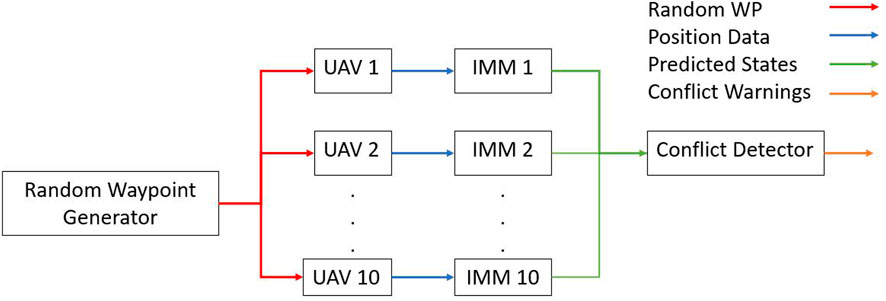
FIGURE 1. Block diagram for proposed system.

3.1 Random recursive simulation setup

To test this system, a random recursive simulation was developed for use in the ROS-Gazebo environment. We are using ten multi-rotor vehicles in the simulation to simulate sUAS operating within a specified airspace. For this system, all vehicles are assigned random unique way-points in a semi-synchronous fashion. The vehicles are semi-synchronous which means new way-points will not be assigned to the vehicles until all of the other vehicles have reached their current respective way-points, however all vehicles arrive at their assigned way-points at different times. After a vehicle arrives at the way-point, it holds the position until a new way-point is received. It may be noted that we took a semi-synchronous approach when developing this simulation for analysis and data collection purposes, and our proposed method does not impose this requirement. The vehicles move in a linear motion between way-points. Based on geometry, a vehicle pair can have a maximum of one conflict per simulation iteration. This holds true even if vehicles are operating on a co-linear trajectory due to the dynamics of the system and the simulation setup. The simulation is continuous with the end of the previous simulation iteration being used as the starting point of the next simulation iteration. A simulation iteration starts with the assignment of the random way-points to the vehicles. A simulation iteration ends once all vehicles have reached their assigned way-points. This approach simulates a way-point navigation mission with multiple way-points and intermediate stops. In addition to simulating a way-point navigation mission, while a vehicle is waiting for its new way-point, it becomes equivalent to a vehicle hovering in the national airspace that other vehicles will still need to avoid. Multi-rotor vehicles moving to a way-point and then hovering at the way-point is a very realistic task for delivery of packages, photography and building inspections, thus making this approach a valid model of the national airspace even with the constraints put in for data collection and analysis purposes. In addition to the way-point messages, the random way-point generator also sends a message once all vehicles have reached their desired way-points. This message is used in the conflict detector as the signal to save the current conflict data. This signal is triggered once all vehicles are within approximately 2 m of the desired way-point.

Algorithm 1: Random Way-point Generator Pseudo Code.

while WP_Count $\le 9$ do

 if All Vehicles at WPs then

  Save Prev. WPs

  Send Complete signal to Conflict Detector

  Generate New Way-points

  WP_count=WP_count+1

 else

  Publish previous WPs

 end if

end while

We use the ROS-Gazebo physics-based engine to simulate multi-rotor systems. The vehicles use the default PX4 way-point and attitude controllers to achieve the desired position and velocity set points. Vehicles are restricted to a maximum horizontal velocity of 12 m/s. The velocity of the aircraft is set by the position controller and is dependent on how far the vehicle is from the way-point.

As previously mentioned in the first paragraph of 3.1, new way-points for the random recursive way-point generator are randomly selected from a continuous uniform distribution. We select latitude and longitude way-points independently from the probability distributions described in Eqs 1, 2. The variables a and b in Eqs 1, 2 are the upper and lower bounds for the latitude and longitude points. The upper and lower latitude bounds we selected were 39.1576569° and 39.150874°. The upper and lower longitude bounds we selected were −84.7832447° and −84.7908162°. The resulting bounded flight area is a .75 km by .65 km rectangle and can be seen in Figure 2.

$\mathit{Prob}.Dist.LatWP=\left\{\begin{array}{cc}\frac{1}{b-a},\hfill & \text{for\hspace{0.17em}}a\le x\le b\hfill \\ 0,\hfill & \text{otherwise}\hfill \end{array}\right.(1)$

$\mathit{Prob}.Dist.LonWP=\left\{\begin{array}{cc}\frac{1}{b-a},\hfill & \text{for\hspace{0.17em}}a\le x\le b\hfill \\ 0,\hfill & \text{otherwise}\hfill \end{array}\right.(2)$

FIGURE 2

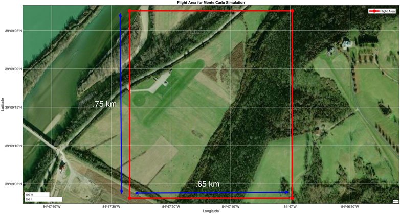
FIGURE 2. Allocated airspace for testing.

While the latitude and longitude way-points were randomly selected, the altitude component of the way-points were manually set and kept constant for each vehicle. The altitude was set manually to ensure separation between the vehicles which allowed them to complete their flights without crashing. Each run of the simulation consisted of the 10 vehicles flying 9 randomly assigned way-points. The vehicles publish their fused GPS-IMU position data as they fly between way-points.

3.2 Interacting multiple model

In this section, we discuss the background information of the interacting multiple model and go through the different sub-modules of the IMM system [please see our previous work Wells et al. (2021a) for details and additional results on this]. The interacting multiple model is a filtering technique for systems with unknown underlying models. It was first developed by Bloom (1984), however its popularity increased after its publication by Bloom and Bar-Shalom (1988). The interacting multiple model we are presenting in this paper is capable of estimating the vehicle’s 9 states shown in Eq. 3. The full 9 states the IMM calculates is for the more general application of this system. For this paper, we are narrowing our focus to only predicting the latitude and longitude position states. The altitude component of the state vector is still being predicted, however, it is not used in the conflict detection process. The IMM can estimate these states through a recursive process where the previous state outputs are used as the new state inputs for each iteration of the IMM. The IMMs are constantly iterating while the simulation is running and the IMM iterations are independent of the simulation iterations discussed in the previous section. In each IMM iteration, the states are mixed based on previous model probability, updated and corrected through a position measurement, and then mixed again. The probability based mixing and model updating is accomplished through several different sub-modules which can be seen in Figure 3. The system consists of a state pre-mixing sub-module, three independent Kalman Filters, model combination sub-module, model probability sub-module and a future position predictor sub-module. The first sub-module in the system is pre-mixing. Pre-mixing uses previous state estimates and the probability of switching models between IMM iterations to regenerate new initial states. These new states and any measurement updates which were received are then used as inputs to the three Kalman filters. The three Kalman filters included in the IMM presented here consist of a constant velocity model, a constant acceleration model and a constant turn model. The Kalman filters generate new state estimates, measurement residuals and covariance matrices for the vehicles current motion. The covariance matrices and measurement residuals from each of the Kalman filters are then passed to the updating model probability sub-module. This module updates the model probability for each motion model generated from the Kalman Filter by calculating the current likelihood state and using the previous model probability. The probability for each model is then used in the state estimate combiner sub-module. This sub-module uses the model probabilities to create the combined state estimates and associated covariances for the system. The mixed state estimate and mixed covariance matrix is then used in the predicting future position sub-module where the state is projected into the near future. The rest of this section covers each of the different sub-modules in more detail and goes through the equations for the system.

$StateVector={\left[lat,lon,alt,\dot{lat},\dot{lon},\dot{alt},\ddot{lat},\ddot{lon},\ddot{alt}\right]}^T(3)$

FIGURE 3

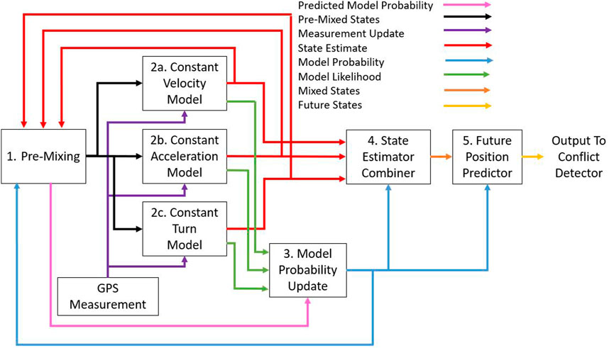
FIGURE 3. Flow chart for interacting multiple model.

3.2.1 Pre-mixing

The first sub-module of the IMM is pre-mixing. The pre-mixing sub-module uses the state estimates and the previous model probabilities as inputs and calculates pre-mixed state and covariance matrix as outputs. Equations 4–7 are the equations for the pre-mixing step. Equation 4 uses the previous model probability $({\mu }_{k-1}^{(j)})$ and a model switching probability (π_ji) to generate three model probability predictions $({\widehat{\mu }}_{k|k-1})$. The indices i and j both range from 1 to 3 and correspond to the three different motion models used later in the Kalman filtering portion of the IMM. The IMM is a recursive function. The subscript k indicates the current time step while k − 1 indicates the previous time step. The model switching probability (π_ji) seen in (4) is a parameter matrix which consists of user defined probabilities that correspond to switching from the current model to a new model or staying with the same model for the next IMM iteration. After finding the predicted model probability, a mixing weight $({\mu }_{k-1}^{j|i})$ is calculated in Eq. 5. The mixing weight calculation uses the previous model probability, the switching probability, and the predicted model probability. The mixing weight is then used as a weighted sum to calculate new, pre-mixed state vector $({\bar{x}}_{kZ|k-1}^{(j)})$ and covariance matrices $({\bar{P}}_{k-1|k-1}^{(j)})$ from the previous state vector r $({\widehat{x}}_{k-1|k-1}^{(j)})$ and covariance matrices $({\widehat{P}}_{k-1|k-1}^{(j)})$ in Eqs 6, 7, respectively. The pre-mixing sub-module passes the pre-mixed model state vector and pre-mixed covariance matrix to the Kalman filter sub-modules. The predicted model probability is passed to the Model Probability sub-module.

${\widehat{\mu }}_{k|k-1}^{\left(i\right)}=\sum _{j=1}^3{\pi }_{ji}{\mu }_{k-1}^{\left(j\right)}(4)$

${\mu }_{k-1}^{j|i}=\frac{{\pi }_{ji}{\mu }_{k-1}^{\left(j\right)}}{{\widehat{\mu }}_{k|k-1}}(5)$

${\bar{x}}_{k-1|k-1}^{\left(i\right)}=\sum _{j=1}^3{\widehat{x}}_{k-1|k-1}^{\left(j\right)}{\mu }_{k-1}^{j|i}(6)$

${\bar{P}}_{k-1|k-1}^{\left(i\right)}=\sum _{j=1}^3\left({\widehat{P}}_{k-1|k-1}^{\left(j\right)}+\cdots {\lambda }_{k-1}{\lambda }_{k-1}^T\right){\mu }_{k-1}^{\left(j|i\right)}(7)$

where, ${\lambda }_{k-1}=({\bar{x}}_{k-1|k-1}^{(i)}-{\widehat{x}}_{k-1|k-1}^{(j)})$.

3.2.2 Kalman filter

The next sub-module in the IMM is the bank of Kalman filters. Variations of the IMM use different filtering techniques such as extended Kalman filters (EKF) (Li and Bar-Shalom, 1993), unscented Kalman filters (UKF) (Gao et al., 2017) or even particle filters (Boers, 2003). We used standard Kalman Filters (KF) for this IMM because we are treating the trajectory models as linear. The three models we are using consist of the constant velocity model, the constant acceleration model, and the constant turn model. In the actual system, the KF process is repeated for each motion model. For brevity, we will go through the KF model once and discuss the different motion models in the subsections below. All three Kalman filters use the mixed state and covariance matrix from the pre-mixing module as inputs. The inputs to the Kalman filter are used in Eqs 8, 9 to find new predicted state vector $({\widehat{x}}_{k|k-1}^{(i)})$ and predicted covarinace matrix $({\widehat{P}}_{\mathrm{k}|\mathrm{k}-1}^{(i)})$. The predictions are found by using a state transition matrix (A). The state transition matrix represents the motion model used in each of the different Kalman filters. The state transition matrix is indexed by “i.” The index i ranges from 1 to 3 and represents the three different motion models used in the IMM. In the state transition matrices, the “dt” term represents the time elapsed since the previous iteration of the Kalman filter. A Gaussian process noise parameter (Q) is added in Eq. 9. State and covariance predictions will continue until a new measurement is received. Once a position measurement from the sUAS is received, the measurement residual $({\tilde{z}}_k^{(i)})$ is calculated in Eq. 10 by finding the difference between the predicted states and the position measurement. The measurement we receive only consists of latitude, longitude, and altitude and not the full state vector. The limited state information received in the measurement update requires the use of an observation matrix (H). The observation matrix is used to only update the states which are directly changed by the measurement. After the measurement residual is calculated, the residual covariance $(S_k^{(i)})$ is found in (11). The residual covariance contains measurement error covariance parameter (R), which attempts to quantify the errors in the measurement. Next, the Kalman gain coefficient $(K_k^{(i)})$ is calculated in Eq. 12 and is used to determine how much the state and covariance matrix will be updated based on the newly received measurement. Finally, the state vector and covariance matrix are updated in Eqs 13, 14, respectively.

${\widehat{x}}_{k|k-1}^{\left(i\right)}=A^{\left(i\right)}{\bar{x}}_{k-1}^{\left(i\right)};\forall i\in \{\mathrm{1,2,3}\}(8)$

${\widehat{P}}_{\mathrm{k}|\mathrm{k}-1}^{\left(i\right)}=A^{\left(i\right)}{P}_{\mathrm{k}-1|\mathrm{k}-1}^{\left(i\right)}{A^{\left(i\right)}}^T+Q(9)$

${\tilde{z}}_k^{\left(i\right)}=z_k-H{\widehat{x}}_{k|k-1}^{\left(i\right)}(10)$

$S_k^{\left(i\right)}=H{\widehat{P}}_{k|k-1}{H}^T+R(11)$

$K_k^{\left(i\right)}={\widehat{P}}_{k|k-1}^{\left(i\right)}{H}^T{\left(S_k^{\left(i\right)}\right)}^{-1}(12)$

${\widehat{x}}_{k|k}^{\left(i\right)}={\widehat{x}}_{k|k-1}^{\left(i\right)}+K_k^{\left(i\right)}{\tilde{z}}_k^{\left(i\right)}(13)$

$P_{k|k}^{\left(i\right)}={\widehat{P}}_{\mathrm{k}|\mathrm{k}-1}^{\left(i\right)}-K_k^{\left(i\right)}{S}_k^{\left(i\right)}{\left(K_k^{\left(i\right)}\right)}^T(14)$

3.2.2.1 Constant velocity model

The state vector and state transition matrix for the constant velocity motion model are shown in Eqs 15, 16. The state vector and state transition matrix consist of latitude (lat), longitude (lon), and altitude (alt) as the base states, the first derivative of the base states and second derivatives of the base states. The constant velocity model uses the first derivative of the base states and assumes the second derivatives are equal to zero. The constant acceleration and constant turn model use all of the states in the state vector. The first three rows of the state transition matrix correspond to the vehicles position. The next three rows correspond to the vehicle’s velocity. The final three rows correspond to the vehicle’s acceleration. The delta time (dt) parameter seen in the state transition matrices comes from the time difference between successive iterations of the Kalman filter.

$x_{\mathit{vel}}={\left[lat,lon,alt,\dot{lat},\dot{lon},\dot{alt},\ddot{lat},\ddot{lon},\ddot{alt}\right]}^T(15)$

$A_{\mathit{vel}}=\left[\begin{array}{ccccccccc}\hfill 1\hfill & \hfill 0\hfill & \hfill 0\hfill & \hfill dt\hfill & \hfill 0\hfill & \hfill 0\hfill & \hfill 0\hfill & \hfill 0\hfill & \hfill 0\hfill \\ \hfill 0\hfill & \hfill 1\hfill & \hfill 0\hfill & \hfill 0\hfill & \hfill dt\hfill & \hfill 0\hfill & \hfill 0\hfill & \hfill 0\hfill & \hfill 0\hfill \\ \hfill 0\hfill & \hfill 0\hfill & \hfill 1\hfill & \hfill 0\hfill & \hfill 0\hfill & \hfill dt\hfill & \hfill 0\hfill & \hfill 0\hfill & \hfill 0\hfill \\ \hfill 0\hfill & \hfill 0\hfill & \hfill 0\hfill & \hfill 1\hfill & \hfill 0\hfill & \hfill 0\hfill & \hfill 0\hfill & \hfill 0\hfill & \hfill 0\hfill \\ \hfill 0\hfill & \hfill 0\hfill & \hfill 0\hfill & \hfill 0\hfill & \hfill 1\hfill & \hfill 0\hfill & \hfill 0\hfill & \hfill 0\hfill & \hfill 0\hfill \\ \hfill 0\hfill & \hfill 0\hfill & \hfill 0\hfill & \hfill 0\hfill & \hfill 0\hfill & \hfill 1\hfill & \hfill 0\hfill & \hfill 0\hfill & \hfill 0\hfill \\ \hfill 0\hfill & \hfill 0\hfill & \hfill 0\hfill & \hfill 0\hfill & \hfill 0\hfill & \hfill 0\hfill & \hfill 0\hfill & \hfill 0\hfill & \hfill 0\hfill \\ \hfill 0\hfill & \hfill 0\hfill & \hfill 0\hfill & \hfill 0\hfill & \hfill 0\hfill & \hfill 0\hfill & \hfill 0\hfill & \hfill 0\hfill & \hfill 0\hfill \\ \hfill 0\hfill & \hfill 0\hfill & \hfill 0\hfill & \hfill 0\hfill & \hfill 0\hfill & \hfill 0\hfill & \hfill 0\hfill & \hfill 0\hfill & \hfill 0\hfill \end{array}\right](16)$

3.2.2.2 Constant acceleration model

The state vector for the constant acceleration model is the same as shown in Eq. 15. The state transition matrix for the constant acceleration model is given by Eq. 17. The constant acceleration model uses the full 9 states in the state vector.

$A_{\mathit{acc}}=\left[\begin{array}{ccccccccc}\hfill 1\hfill & \hfill 0\hfill & \hfill 0\hfill & \hfill dt\hfill & \hfill 0\hfill & \hfill 0\hfill & \hfill \frac{d{t}^2}{2}\hfill & \hfill 0\hfill & \hfill 0\hfill \\ \hfill 0\hfill & \hfill 1\hfill & \hfill 0\hfill & \hfill 0\hfill & \hfill dt\hfill & \hfill 0\hfill & \hfill 0\hfill & \hfill \frac{d{t}^2}{2}\hfill & \hfill 0\hfill \\ \hfill 0\hfill & \hfill 0\hfill & \hfill 1\hfill & \hfill 0\hfill & \hfill 0\hfill & \hfill dt\hfill & \hfill 0\hfill & \hfill 0\hfill & \hfill \frac{d{t}^2}{2}\hfill \\ \hfill 0\hfill & \hfill 0\hfill & \hfill 0\hfill & \hfill 1\hfill & \hfill 0\hfill & \hfill 0\hfill & \hfill dt\hfill & \hfill 0\hfill & \hfill 0\hfill \\ \hfill 0\hfill & \hfill 0\hfill & \hfill 0\hfill & \hfill 0\hfill & \hfill 1\hfill & \hfill 0\hfill & \hfill 0\hfill & \hfill dt\hfill & \hfill 0\hfill \\ \hfill 0\hfill & \hfill 0\hfill & \hfill 0\hfill & \hfill 0\hfill & \hfill 0\hfill & \hfill 1\hfill & \hfill 0\hfill & \hfill 0\hfill & \hfill dt\hfill \\ \hfill 0\hfill & \hfill 0\hfill & \hfill 0\hfill & \hfill 0\hfill & \hfill 0\hfill & \hfill 0\hfill & \hfill 1\hfill & \hfill 0\hfill & \hfill 0\hfill \\ \hfill 0\hfill & \hfill 0\hfill & \hfill 0\hfill & \hfill 0\hfill & \hfill 0\hfill & \hfill 0\hfill & \hfill 0\hfill & \hfill 1\hfill & \hfill 0\hfill \\ \hfill 0\hfill & \hfill 0\hfill & \hfill 0\hfill & \hfill 0\hfill & \hfill 0\hfill & \hfill 0\hfill & \hfill 0\hfill & \hfill 0\hfill & \hfill 1\hfill \end{array}\right](17)$

3.2.2.3 Constant turn model

The state vector for the constant turn model is the same as shown in Eq. 15. The state transition matrix for the constant turn model is given by Eq. 17. The constant turn model [seen in Genovese (2001)] is similar to the constant acceleration model as it uses the full nine states. The constant turn model differs from the constant acceleration model as it assumes the vehicle is turning at a constant rate (ω) and speed. The acceleration portion of the constant turn model causes a change in direction and not a change in vehicle speed. The state transition matrix can be seen in Eq. 19 and models the constant turn dynamics.

$\omega =\frac{\sqrt{{\ddot{lat}}^2+{\ddot{lon}}^2}}{\sqrt{{\dot{lat}}^2+{\dot{lon}}^2}}(18)$

$A_t=\left[\begin{array}{ccccccccc}\hfill 1\hfill & \hfill 0\hfill & \hfill 0\hfill & \hfill A_t^{14}\hfill & \hfill 0\hfill & \hfill 0\hfill & \hfill A_t^{17}\hfill & \hfill 0\hfill & \hfill 0\hfill \\ \hfill 0\hfill & \hfill 1\hfill & \hfill 0\hfill & \hfill 0\hfill & \hfill A_t^{25}\hfill & \hfill 0\hfill & \hfill 0\hfill & \hfill A_t^{28}\hfill & \hfill 0\hfill \\ \hfill 0\hfill & \hfill 0\hfill & \hfill 1\hfill & \hfill 0\hfill & \hfill 0\hfill & \hfill A_t^{36}\hfill & \hfill 0\hfill & \hfill 0\hfill & \hfill 0\hfill \\ \hfill 0\hfill & \hfill 0\hfill & \hfill 0\hfill & \hfill A_t^{44}\hfill & \hfill 0\hfill & \hfill 0\hfill & \hfill A_t^{47}\hfill & \hfill 0\hfill & \hfill 0\hfill \\ \hfill 0\hfill & \hfill 0\hfill & \hfill 0\hfill & \hfill 0\hfill & \hfill A_t^{55}\hfill & \hfill 0\hfill & \hfill 0\hfill & \hfill A_t^{58}\hfill & \hfill 0\hfill \\ \hfill 0\hfill & \hfill 0\hfill & \hfill 0\hfill & \hfill 0\hfill & \hfill 0\hfill & \hfill 1\hfill & \hfill 0\hfill & \hfill 0\hfill & \hfill 0\hfill \\ \hfill 0\hfill & \hfill 0\hfill & \hfill 0\hfill & \hfill A_t^{74}\hfill & \hfill 0\hfill & \hfill 0\hfill & \hfill A_t^{77}\hfill & \hfill 0\hfill & \hfill 0\hfill \\ \hfill 0\hfill & \hfill 0\hfill & \hfill 0\hfill & \hfill 0\hfill & \hfill A_t^{85}\hfill & \hfill 0\hfill & \hfill 0\hfill & \hfill A_t^{88}\hfill & \hfill 0\hfill \\ \hfill 0\hfill & \hfill 0\hfill & \hfill 0\hfill & \hfill 0\hfill & \hfill 0\hfill & \hfill 0\hfill & \hfill 0\hfill & \hfill 0\hfill & \hfill 0\hfill \end{array}\right](19)$

$\begin{array}{ll}\hfill S& ≔\mathit{sin}\left(\right);C≔\mathit{cos}\left(\right);\hfill \\ \hfill A_t^{14}& =\frac{S\left(\omega dt\right)}{\omega };A_t^{17}=\frac{\left(1-C\left(\omega dt\right)\right)}{{\omega }^2};\hfill \\ \hfill A_t^{25}& =\frac{S\left(\omega dt\right)}{\omega };A_t^{28}=\frac{\left(1-C\left(\omega dt\right)\right)}{{\omega }^2};\hfill \\ \hfill A_t^{36}& =dt;A_t^{44}=C\left(\omega dt\right);A_t^{47}=\frac{S\left(\omega dt\right)}{\omega };\hfill \\ \hfill A_t^{55}& =C\left(\omega dt\right);A_t^{58}=\frac{S\left(\omega dt\right)}{\omega }\hfill \\ \hfill A_t^{74}& =-\omega S\left(\omega dt\right);A_t^{77}=C\left(\omega dt\right);\hfill \\ \hfill A_t^{85}& =-\omega S\left(\omega dt\right);A_t^{88}=C\left(\omega dt\right)\hfill \end{array}$

3.2.3 Model probability update

The model probability update is the next sub-module after the Kalman filters have generated new state vectors, covariance matrices and measurement residuals. The model probability update is completed in two steps. The first step is the calculation of the likelihood for each of the different motion models. The model likelihood is based on the measurement residual and the residual covariances found in the previous Kalman filters. The equation for model likelihood is shown in Eq. 20. After the model likelihood is calculated, the model probability for each model is found in Eq. 21.

$L_k^i=\frac{e^{-1/2{\left({\tilde{z}}_k^{\left(i\right)}\right)}^T{\left(S_k^{\left(i\right)}\right)}^{-1}{\tilde{z}}_k^{\left(i\right)}}}{\det {\left(2\pi S_k^i\right)}^{1/2}}(20)$

${\mu }_k^{\left(i\right)}=\dots \frac{{\widehat{\mu }}_{k|k-1}^{\left(i\right)}{L}_k^{\left(i\right)}}{{\sum }_{j=1}^3{\widehat{\mu }}_{k|k-1}^{\left(j\right)}{L}_k^{\left(j\right)}};\forall i\in \{\mathrm{1,2,3}\}(21)$

3.2.4 State estimator combiner

The next sub-module in the IMM is the state estimator combiner. The state estimate combiner creates weighted averages of all of the state vectors and covariance matrices created from the three Kalman Filters. The model probabilities calculated in the model probability update sub-module are used as the weights. Models that have a higher probability of being the correct model contribute to the final mixed states more than models which have lower probabilities. The equations for calculating the mixed state vector and covariance matrix are shown in Eqs 22, 23.

$x_{k|k}=\sum _{i=1}^3{\widehat{x}}_{k|k}^{\left(i\right)}{\mu }_k^{\left(i\right)}(22)$

$P_{k|k}=\sum _{i=1}^3\left[P_{k|k}^{\left(i\right)}+\left(x_{k|k}-{\widehat{x}}_{k|k}^{\left(i\right)}\right){\left(x_{k|k}-{\widehat{x}}_{k|k}^{\left(i\right)}\right)}^T\right]{\mu }_k^{\left(i\right)}(23)$

3.2.5 Future position predictor

The final sub-module of the IMM system presented here is the future position predictor. The future position predictor uses the model probabilities calculated in the model probability update sub-module and the mixed state and covariance matrix found in the state estimate combiner sub-module to find near-future state estimates for a vehicle in flight. The near-future state and covariance estimates are found by selecting the motion model with the highest probability and then applying it to the mixed state and covariance matrix. The near future estimates for the mixed state and covariance matrices are generated by setting the dt value the desired future time estimate. Several future time estimates are generated to create a prediction track. As the model is projected further into the future, the uncertainty of the system increases and its accuracy decreases. The decrease in accuracy is expected as we are only using the limited positional information from the measurement and do not have any information on vehicle intent. The future position prediction equations for the state vector and covariance matrix can be seen in Eqs 24, 25. The predictions shown in Eqs 24, 25 are constantly being updated for each vehicles. The predictions are a sliding window, constantly looking up to 20 s into the future from the current simulation time (t₀).

$x_{\mathit{future}}=A_{\max \left({\mu }_k\right)}{x}_{k|k}(24)$

$P_{\mathit{future}}=A_{\max \left({\mu }_k\right)}{P}_{\mathrm{k}|\mathrm{k}}{A}_{\max \left({\mu }_k\right)}^T+R(25)$

3.3 Haversine-based conflict detector

The Haversine conflict detector is a geometric based conflict detector that uses the stream of future position predictions of the IMM as inputs. This algorithm uses the Law of Haversines to estimate the distance between the predicted latitude/longitude coordinates of two sUAS’. The estimation distance is based on the great circle distance. The Haversine algorithm assumes the Earth a perfect sphere and calculates the distance between the points on the surface. This assumption can be seen in Eq. 30 by using the radius of the Earth in meters. The assumption that the Earth is a perfect sphere does lead to some errors in the calculated distance. This does not create an issue though because the distances between vehicles we are concerned with are relatively small, and the distance error grows as points are farther apart. In this application, we are using the estimate to find the distance between vehicles in meters. As seen in Figure 4, the Haversine algorithm is applied to points within the same prediction window to calculate the straight line distance between vehicles. We are comparing where the vehicles are at different time steps in the near-future to see if the distance falls below a conflict threshold value. As stated in the problem formulation section, a conflict occurs when the distance between two vehicles falls below 5 m in the current time frame. To try and predict when a conflict occurs based on the future position, additional threshold values were set for the different prediction windows. The thresholds increase as the prediction time increases due to the uncertainty within the prediction. These thresholds were set based on sensitivity studies performed. The equations for the Haversine algorithm are provided in (26–37). Equations 26–29 show the latitude and longitude components being converted from degrees to radians. Equations 31, 32 calculate the differences between the points. Equations 33, 34 show the calculation of the great circle distance the Haversine formula is based on. For the work presented here, we have omitted Eq. 35 as we have ensured altitude separation. In practice either Eq. 35 could be implemented or vertical separation could be considered a different restriction entirely. In addition to identifying conflicts, we are also able to provide an estimated conflict location with the conflict detector. The estimated conflict location is found only if the lateral distance calculated in (34) is less than the threshold value that is set for that prediction window. To find the estimated conflict latitude and longitude, we take the average of both vehicles predicted locations as seen in (36) and (37).

${\varphi }_1=la{t}_1\ast \pi /180(26)$

${\varphi }_2=la{t}_2\ast \pi /180(27)$

${\lambda }_1=lo{n}_1\ast \pi /180(28)$

${\lambda }_2=lo{n}_2\ast \pi /180(29)$

$R=6371000(30)$

$\mathrm{\Delta }\varphi ={\varphi }_2-{\varphi }_1(31)$

$\mathrm{\Delta }\lambda ={\lambda }_2-{\lambda }_{1}a=S{\left(\mathrm{\Delta }\varphi /2\right)}^2+C\left({\varphi }_1\right)\ast \dots C\left({\varphi }_2\right)\ast s{\left(\mathrm{\Delta }\lambda /2\right)}^2(32)$

$d=2\ast atan2\left(sqrt\left(a\right),sqrt\left(1-a\right)\right)(33)$

$Dis{t}_{\mathit{Lateral}}=R\ast d(34)$

$Dis{t}_{\mathit{Total}}=sqrt\left(Dis{t}_{\mathit{Lateral}}^2+{\left(al{t}_1-al{t}_2\right)}^2\right)(35)$

$la{t}_{\mathit{est.conflict}}=\left(la{t}_1+la{t}_2\right)/2(36)$

$lo{n}_{\mathit{est.conflict}}=\left(lo{n}_1+lo{n}_2\right)/2(37)$

$S≔\mathit{sin}\left(\right);C≔\mathit{cos}\left(\right);$

FIGURE 4

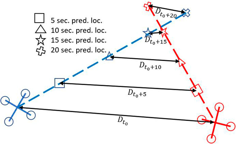
FIGURE 4. Conflict detection diagram.

As previously stated and shown in Figure 4, we apply the Haversine algorithm between predicted points in the same time window. If a prediction falls below the threshold value for the prediction time window, a conflict will likely occur, and the data is saved. We record the conflict data in a conflict detection matrix that gets saved to a csv file and then reset at the end of each simulation iteration. Each prediction time frame has its own conflict detection matrix. The conflict matrices can either have values of zero or one. A zero indicates there has not been a conflict between the two sUAS in that given simulation iteration while a one indicates there was a conflict. A conflict between vehicles is only counted once per simulation iteration, even if the conflict appears multiple times as the prediction window shifts. In addition to the prediction conflict matrices, we also record a true conflict matrix. The true conflict matrix is similar to the prediction conflict matrices except it records any time two vehicles fall below the 5 m threshold value. This is what we use to determine how many conflicts did occur.

4 Results

The system we created was tested with the random recursive way-point generator and consisted of interacting multiple models and a Haversine-based conflict detector. An interacting multiple model was running for each aircraft operating within the simulation. The IMM was producing path predictions for each of the vehicles while they were in flight. An example of the path predictions the IMM is producing can be seen in Figure 5. As can be seen in Figure 5, when the predictions are further into the future, the accuracy decreases. This is due to the lack of intent information being provided to the IMM about a highly dynamic system. The accuracy for the predictions further in the future especially decreases when a vehicle turns because of the lack of information about an upcoming highly nonlinear maneuver.

FIGURE 5

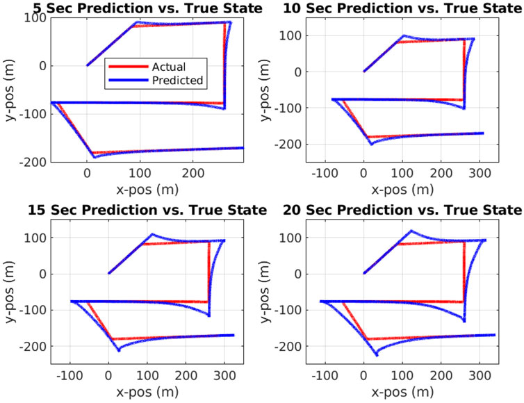
FIGURE 5. Results for IMM path predictor.

After the IMM was developed and tested using user defined way-points through QGroundControl, the Haversine conflict detector was then tested using the random recursive way-point generator and the results are presented in Figures 6–12. The results were generated for 10 aircraft. Each aircraft was assigned 9 way-points in a given simulation and 5 simulations were completed. This resulted in 450 individual way-point flights. Multiple instances of the 450 flights were completed to tune the future conflict threshold value within the Haversine conflict predictor. When tuning the thresholds, our goal was to be able to accurately detect true conflicts while also minimizing the number of false positive conflicts detected. The threshold values that we found worked the best were: 12 m for the 5 s prediction, 14 m for the 10 s predictions, 16 m for 15 s predictions and 18 m for 20 s predictions. These values were found on a trial-and-error basis. We looked at how many conflicts were detected in each prediction window. We expected to see a downward trend of conflicts starting from high prediction windows to lower with 5 s being the most accurate when compared to the true number of conflicts. If the threshold value for each prediction window was decreased too much, then future conflicts would be missed. If the threshold value for each prediction window was increased it too much, it would detect too many false positives.

FIGURE 6

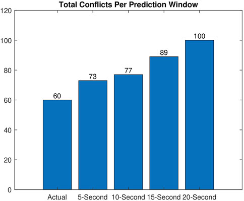
FIGURE 6. Conflicts per predicted time window.

FIGURE 7

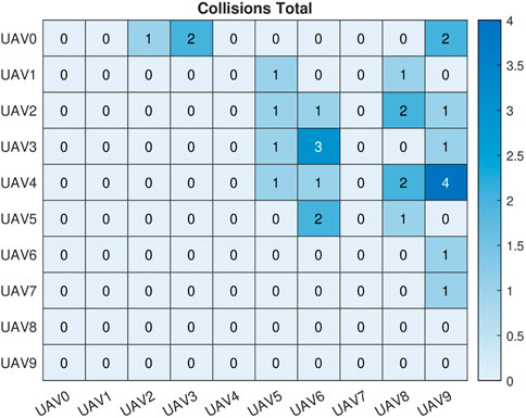
FIGURE 7. Conflict Map t = 0.

FIGURE 8

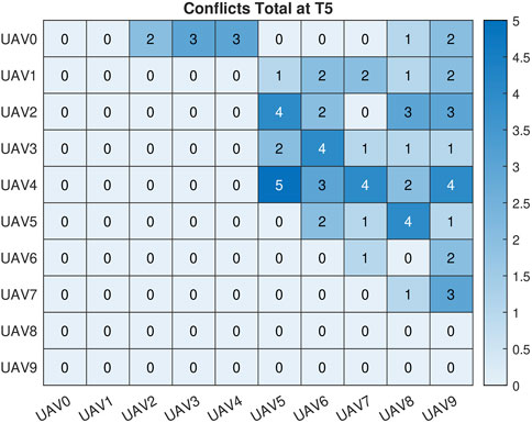
FIGURE 8. Conflict Map t = 5.

FIGURE 9

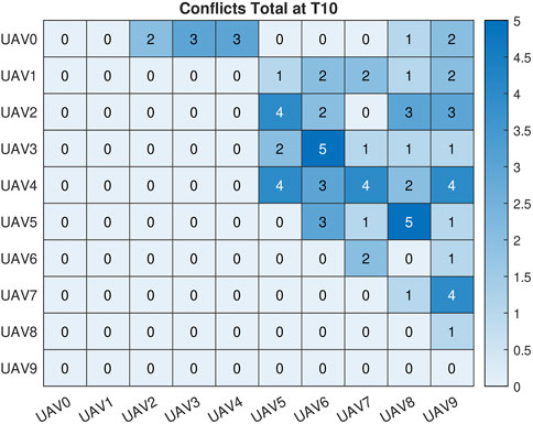
FIGURE 9. Conflict Map t = 10.

FIGURE 10

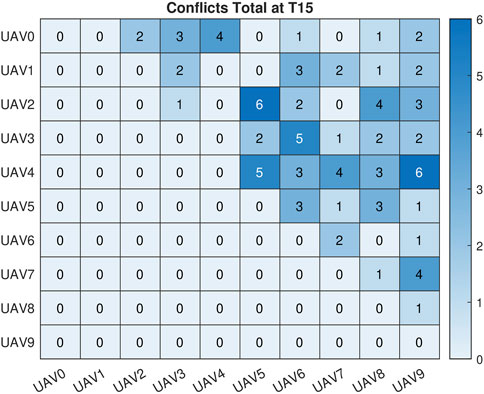
FIGURE 10. Conflict Map t = 15.

FIGURE 11

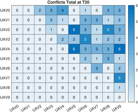
FIGURE 11. Conflict Map t = 20.

FIGURE 12

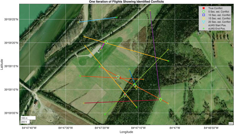
FIGURE 12. Map of identified conflicts for one way-point.

The total number of conflicts for each of the prediction windows can be seen in Figure 6. The combined IMM and Haversine conflict detector identified: 100 conflicts using the 20 s path prediction data, 89 conflicts using the 15 s path prediction data, 77 conflicts using the 10 s prediction data and 73 conflicts for the 5 s prediction data. There were 60 conflicts that occurred based on the 5 m threshold we had set. The discrepancy in the number of conflicts was expected due to the previously discussed degradation of accuracy of the IMM for predictions that occur further in the future. Even with this decreased accuracy, we were able to detect all of the conflicts that actually occurred. In addition to the bar graph showing the number of conflicts, Figures 7–11 are the conflict maps which contain the vehicle vs. vehicle conflict counts for all 450 flights. To read Figures 7–11, select a vehicle on the X-axis and a vehicle on the Y-axis. The number in the corresponding box is the total number of conflicts between the two vehicles for the full 450. For example, in Figure 7, UAV 0 and UAV 3 had a total of 2 conflicts during all 450 flights. The conflict maps were initially a symmetric matrix about main diagonal; however, the lower triangle was removed. Prior to the removal of the lower triangle portion of the conflict map, each conflict showed up twice in the matrix, once in the UAV (X,Y) position and then again in the UAV (Y,X) position. Removing the lower triangle was done for visualization purposes and so conflicts would not show up twice. When comparing Figures 8–11 to Figure 7, it can be noted that all of the conflicts that showed up in Figure 7 had shown up in future position predictions. Based on the way we have set up the simulation and data recording, we have eliminated the chance of missing true conflicts. This was done by constantly recording and updating the minimum Haversine distance between all vehicles for each simulation iteration. With this approach and the results obtained, we can say with certainty that all of the conflicts that actually occurred did show up in the later prediction windows.

Figure 12 shows the results of a set of 10 vehicles flying between two way-points. Conflicts have been identified and appropriately labeled based on the time prediction window in which they were detected, and the conflict’s corresponding predicted location was plotted. As seen in the collision matrices, the majority of the conflicts identified showed up again in decreasing time prediction windows as the vehicle flew along its path. As an example, assume that a conflict is initially detected using the 20 s path prediction. Based on the data shown, the same conflict will likely show up again in the 15 s prediction window after the vehicle travels for approximately 5 s. This result shows that the IMM is predicting future positions of the vehicles accurately (especially as prediction time decreases) and the conflict detector is consistently identifying conflicts. Some miss identification of collisions will occur due to the IMM’s degradation of accuracy for predictions further in the future, however another source of miss identification of conflicts is due to vehicles stopping upon reaching their way-point. If two vehicles are in a pending conflict, and one stops because it reached its way-point, the previously identified conflict was still recorded and counts for the prediction window in which it was identified. With the current simulation setup, the conflict detector counts any conflicts that occur, even if it is caused by one iteration of the IMM that produced inaccurate results.

5 Conclusion and future work

This paper presented the development and application of an IMM based future path predictor coupled with a Haversine-based conflict detector. The proposed system generated path predictions with the IMM and then identified likely conflicts in the near-future with the Haversine-based conflict detector. This was done in real-time as vehicles fly randomly generated way-points in the NAS. The system will facilitate sUAS operations within the NAS by identifying conflicts before they occur which will give vehicles more time to re-route. The paper presented the development of the random recursive way-point generator used for testing, the different sub-modules of the interacting multiple model, and finally went through the derivation of the Haversine-based conflict detector. The system was tested with 10 vehicles in a ROS-Gazebo framework. The results showed the system was able to effectively identify conflicts with the future position predictions. The results were presented in vehicle vs. vehicle conflict maps and a map of the predicted conflicts as vehicles flew. Going forward, we aim to develop a re-routing module which can mitigate the detected conflicts so vehicles will be able to operate safely within the national airspace.

Data availability statement

The raw data supporting the conclusion of this article will be made available by the authors, without undue reservation.

Author contributions

JW conceived, developed, and presented the theory behind this work. MK provided guidance and supervision to the work as it was developed. JW and MK discussed the findings presented in this paper. JW wrote the manuscript and MK reviewed it prior to submission and publication. All authors contributed to the article and approved the submitted version.

Funding

This research has been conducted as part of JW’s PhD dissertation as a graduate student at the University of Cincinnati.

Conflict of interest

The authors declare that the research was conducted in the absence of any commercial or financial relationships that could be construed as a potential conflict of interest.

Publisher’s note

All claims expressed in this article are solely those of the authors and do not necessarily represent those of their affiliated organizations, or those of the publisher, the editors and the reviewers. Any product that may be evaluated in this article, or claim that may be made by its manufacturer, is not guaranteed or endorsed by the publisher.

References

Bloom, H. A. P., and Bar-Shalom, Y. (1988). The interacting multiple model algorithm for systems with markovian switching coefficients. IEEE Trans. Automatic Control 33, 780–783. doi:10.1109/9.1299

CrossRef Full Text | Google Scholar

Bloom, P. (1984). “An efficient filter for abruptly changing systems,” in The 23rd IEEE conference on decision and control, 656–658.

Google Scholar

Boers, Y., and Driessen, J. (2003). Interacting multiple model particle filter. IEE Proc. - Radar, Sonar Navigation 150 (5), 344–349. doi:10.1049/ip-rsn:20030741

CrossRef Full Text | Google Scholar

Cao, Y., Rathinam, S., and Sun, D. (2011). A rescheduling method for conflict-free continuous descent approach. doi:10.2514/6.2011-6218

CrossRef Full Text | Google Scholar

Chakrabarty, A., Stepanyan, V., Krishnakumar, K. S., and Ippolito, C. A. (2019). “Real-time path planning for multi-copters flying in utm-tcl4,” in AIAA scitech 2019 forum, 0958.

CrossRef Full Text | Google Scholar

Conte, C., de Alteriis, G., Schiano Lo Moriello, R., Accardo, D., and Rufino, G. (2021). Drone trajectory segmentation for real-time and adaptive time-of-flight prediction. Drones 5, 62. doi:10.3390/drones5030062

CrossRef Full Text | Google Scholar

Costea, M.-L., Nae, C., Apostolescu, N., Costache, F., Andrei, I.-C., Stroe, G.-L., et al. (2020). “Automatic aircraft collisions algorithm development for civil aircraft,” in 2020 10th international conference on advanced computer information technologies (ACIT), 98–103. doi:10.1109/ACIT49673.2020.9208865

CrossRef Full Text | Google Scholar

FAA (2022). FAA aerospace forecast fiscal years 2022-2042, 36, 41–63.

Google Scholar

Fabra, F., Calafate, C. T., Cano, J. C., and Manzoni, P. (2018). “A collision avoidance solution for UAVs following planned missions,” in 2018 IEEE Wireless Communications and Networking Conference Workshops (WCNCW), Barcelona, Spain, 55–60. doi:10.1109/WCNCW.2018.8368977

CrossRef Full Text | Google Scholar

Filippis, L. D., and Guglieri, G. (2012). “Advanced graph search algorithms for path planning of flight vehicles,” in Recent advances in aircraft technology. Editor R. K. Agarwal (Rijeka: IntechOpen). doi:10.5772/37033

CrossRef Full Text | Google Scholar

Galea, M., Zammit, B., and Gauci, J. (2018). “Design of a multi-layer uav path planner for cluttered environments,” in 2018 international conference on unmanned aircraft systems (ICUAS), 914–923. doi:10.1109/ICUAS.2018.8453481

CrossRef Full Text | Google Scholar

Gao, B., Gao, S., Zhong, Y., Hu, G., and Gu, C. (2017). Interacting multiple model estimation-based adaptive robust unscented kalman filter. Int. J. Control, Automation Syst. 15, 2013–2025. doi:10.1007/s12555-016-0589-2

CrossRef Full Text | Google Scholar

Genovese, A. F. (2001). The interacting multiple model algorithm for accurate state estimation of maneuvering targets. Johns Hopkins Apl. Tech. Dig. 22, 614–623.

Google Scholar

Kim, H., Park, C., Lee, S., and Lee, D. (2021a). “Collision avoidance based on CPA algorithm using relative distance and azimuth of radar for unmanned aerial vehicles,” in 2021 21st International Conference on Control, Automation and Systems (ICCAS), Jeju, Republic of Korea, 534–538. doi:10.23919/ICCAS52745.2021.9650061

CrossRef Full Text | Google Scholar

Kim, J.-H., Briceno, S. I., Justin, C. Y., and Mavris, D. (2021b). Designated points-based free-flight approach to enable real-time flight path planning. doi:10.2514/6.2021-2403

CrossRef Full Text | Google Scholar

Kim, J.-H., Zhang, C., Briceno, S. I., and Mavris, D. N. (2021c). Supervised machine learning-based wind prediction to enable real-time flight path planning. doi:10.2514/6.2021-0519

CrossRef Full Text | Google Scholar

Kraus, T. (2008). The federal aviation administration” a historical perspective, 1903–2008.

Google Scholar

Li, X., and Bar-Shalom, Y. (1993). Design of an interacting multiple model algorithm for air traffic control tracking. IEEE Trans. Control Syst. Technol. 1, 186–194. doi:10.1109/87.251886

CrossRef Full Text | Google Scholar

Nagchaudhuri, A., Mitra, M., Hartman, C., Ford, T., and Pandya, J. (2018). “Mobile robotic platforms to support smart farming efforts at umes,” in 2018 14th IEEE/ASME international conference on mechatronic and embedded systems and applications (MESA), 1–7. doi:10.1109/MESA.2018.8449182

CrossRef Full Text | Google Scholar

Ni, J., Wang, X., Tang, M., Cao, W., Shi, P., and Yang, S. X. (2020). An improved real-time path planning method based on dragonfly algorithm for heterogeneous multi-robot system. IEEE Access 8, 140558–140568. doi:10.1109/ACCESS.2020.3012886

CrossRef Full Text | Google Scholar

Qu, J., Gan, X., Zhao, G., and Chen, S. (2019). “Research on detection and warning of air threat situation for uav collision avoidance,” in 2019 international conference on intelligent computing, automation and systems (ICICAS), 226–229. doi:10.1109/ICICAS48597.2019.00055

CrossRef Full Text | Google Scholar

Venkatesh, C., Balasubramaniam, A., Kumar, R., Brown, B., Norouzi, M., Helmicki, A., et al. (2018). Construction site evaluation employing 3d models from uav imagery, 227–233. doi:10.32548/RS.2018.006

CrossRef Full Text | Google Scholar

Wang, Y., zhao, S., Wang, X., and Shen, L. (2019). “A novel collision avoidance method for multiple fixed-wing unmanned aerial vehicles,” in 2019 Chinese automation congress (CAC), 3621–3626. doi:10.1109/CAC48633.2019.8996560

CrossRef Full Text | Google Scholar

Wells, J. Z., Kumar, R., and Kumar, M. (2021a). “Application of interacting multiple model for future state prediction of small unmanned aerial systems,” in 2021 American control conference (ACC), 3755–3760. doi:10.23919/ACC50511.2021.9482778

CrossRef Full Text | Google Scholar

Wells, J. Z., Kumar, R., and Kumar, M. (2021b). Implementation of multiple model: Simulation and experimentation for future state prediction on different classes of small unmanned aerial systems.

Google Scholar

Wyngaard, J., Rund, S. S., Madey, G. R., Vierhauser, M., and Cleland-Huang, J. (2018). “Poster: Swarming remote piloted aircraft systems for mosquito-borne disease research and control,” in 2018 IEEE/ACM 40th international conference on software engineering: Companion (ICSE-Companion), 226–227.

Google Scholar

Zollars, M. D., Cobb, R. G., and Grymin, D. J. (2018). “Optimal path planning for suas waypoint following in urban environments,” in 2018 IEEE Aerospace conference, 1–8. doi:10.1109/AERO.2018.8396483

CrossRef Full Text | Google Scholar

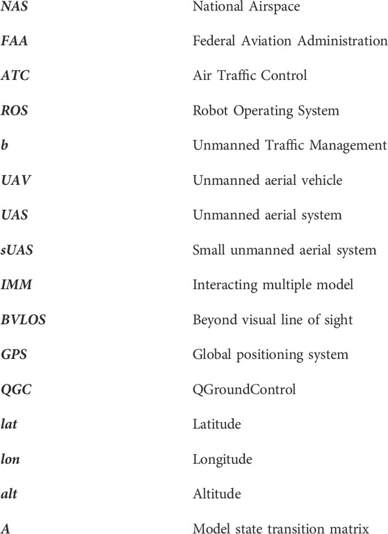
Nomenclature