Trajectory generation based on power for urban air mobility

1 Introduction

The developing concept and technology of Urban Air Mobility (UAM) has the potential to revolutionize short-range air travel in densely populated urban areas (Thipphavong et al., 2018; Urban Air Mobility, 2020; Goodrich and Theodore, 2021; Hill et al., 2021). Many airframe developers, both new and old, are developing new electric aircraft models capable of vertical takeoff and landing (eVTOL) for UAM. Although none of these vehicles are yet certified by the FAA, the ultimate vision is to have thousands of them in the sky during commuting hours in major metropolitan areas. The challenges are daunting, however, and the most critical challenges pertain to safety. Public acceptance will require that catastrophic accidents be extremely rare.

In the early stages of the development, traffic densities will be low, and the main safety concerns will be the airworthiness of individual vehicles and keeping them safely in flight and away from static obstacles. As traffic density increases, however, the safety concerns will shift to the traffic and the potential for mid-air collisions. The development of an air traffic control (ATC) system for UAM will certainly require extensive simulation studies, and those studies will require flight modeling and simulation.

The fidelity of aircraft flight modeling forms a spectrum from low to high. Typically, a lower level of fidelity is required for modeling air traffic than is required for engineering development of a particular model of vehicle. Vehicle engineering and control system design usually requires a detailed model with six or more degrees of freedom, including controls and actuators, whereas traffic modeling for ATC development and simulation testing as well as actual operations (including conflict detection and resolution) in the field usually only requires a simpler point-mass model (Zhang et al., 2010; Chatterji, 2020; Shaw-Lecerf et al., 2020).

This paper proposes an even simpler method of constructing realistic trajectories without the need for a simulation model of the aircraft and its flight controls. This method allows the user to directly specify the route, the static longitudinal profile (altitude as a function of distance), and a power model to determine the progress in time along that profile. The power model can be determined from a recorded or simulated trajectory of the same aircraft type. This capability allows a trajectory to be “bent” into any desired shape while retaining the same basic flight performance characteristics. To the best of the author’s knowledge, this capability has not been proposed in previous literature on trajectory generation.

This method of trajectory generation is useful for several reasons. Aircraft designers are often unwilling to provide detailed simulation models of their aircraft, but this method does not require one. And even if such a model is available, determining the controls to fly a specific trajectory in 4D space is not simple, but this method does not require that to be done. Given a sample of a recorded or a simulated trajectory, it can be used to directly generate a flyable trajectory for conflict resolution. For many conflicts, this method also facilitates the construction of a conflict-free path in 3D space using altitude separation, with no dependence on the timing along the path.

The methods used in this paper are based in part on the Trajectory Specification (TS) concept (Paielli and Erzberger, 2019; Paielli, 2022). TS is a method of specifying a trajectory with explicit tolerances relative to a reference trajectory such that the position at any given time in flight is constrained to a precisely defined volume of space as shown in Figure 1. The reference trajectory is specified as a position in 3D space as a function of time, where the time steps between discrete points can vary, typically being larger in steady-state flight than during transients. The bounding volume at any given time in flight is determined by tolerances relative to the reference trajectory in all three route-oriented axes: cross-track, vertical, and along-track. The tolerances can vary as a function of distance along the route, typically increasing for departure and decreasing for arrival (for conventional aviation).

FIGURE 1

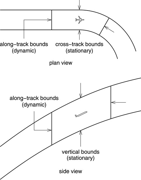
FIGURE 1. Top: Plan view of trajectory bounds in the horizontal plane; Bottom: Side view of trajectory bounds in the longitudinal plane.

That allowance for varying time steps in TS is used in this paper to set the specified power level for the airspeed at that time. The user provides the power function (power as a function of airspeed) that is appropriate for the aircraft and the flight mission. The time steps between discrete points in 3D space are then computed to yield the speed corresponding to the required power. The TS software then automatically converts to a specified constant time step by interpolating between the varying time steps. The resulting uniform time steps allow for fast (constant time) lookup of flight variables as a function of time by simple array indexing, followed by interpolation between the two bounding points for better accuracy than just choosing the nearest point.

The next section discusses the method of generating trajectories based on power for conventional fixed-wing and eVTOL aircraft. Section 3 presents the algorithm for generating the trajectories, and Section 4 analyzes the dependence of trip flight time on the various parameters used in generating the trajectory. Finally, conclusions are presented, followed by a brief Appendix A on solving for the roots of a cubic (third-order) polynomial.

2 Trajectory generation based on power

For any aircraft type, steady flight at a given altitude and airspeed requires a certain amount of power to maintain. That power ultimately comes from the engines or batteries, and it can be applied to the vehicle through either direct thrust, propellers, rotors, or lift, depending on the aircraft type. Any power beyond what is needed to maintain steady state that is not wasted as thermal energy and drag goes into mechanical energy, which is comprised of potential energy due to altitude and kinetic energy due to speed. That “net” or “excess” power is the rate of change of mechanical energy and integrates over time to determine mechanical energy in terms of speed and altitude.

For most aircraft types, the maximum available net power increases with airspeed to some maximum, because it depends on the mass flow through the engines or rotors, then it decreases as drag increases at higher speeds. Maximum available power at takeoff is usually less than it is in forward flight up to some speed. For example, Figure 2 shows the maximum rate of climb as a function of airspeed for the NASA Reference Quadrotor six-passenger air taxi at a pressure altitude of 6,000 ft, as computed by the NASA Design and Analysis of Rotorcraft (NDARC) program (Johnson, 2015; Silva et al., 2018). The rate of climb reaches a maximum of slightly less than 2000 fpm at an airspeed between 50 and 60 knots, and the maximum airspeed is approximately 120 knots.

FIGURE 2

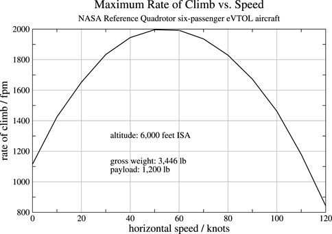
FIGURE 2. Maximum rate of climb as a function of horizontal airspeed for the NASA Reference Quadrotor six-passenger eVTOL aircraft.

To avoid confusion, it should be pointed out that the net or excess power referred to here is not based on the maximum available power. It is based on the power that is appropriate for the aircraft and the mission at any given time, position, and airspeed. In steady-state flight, the net power is zero by definition. For climb, it can range from slightly above zero to maximum power minus the power needed for steady-state flight at the current airspeed and altitude. For descent it is negative. For reliable flight control, it is usually wise to maintain a margin below maximum power so that power can be increased through feedback when necessary to compensate for modeling errors, including wind modeling errors in particular.

A net power model for any trajectory can be derived from recorded or simulated trajectory data by simply computing the rate of change of mechanical energy as a function of airspeed and any other flight variable of interest. The resulting model will depend on how the aircraft was flown, however, so the trajectory that is used should not have arbitrary maneuvers that would not normally be used in flight with no other traffic in the airspace. Note also that when a new trajectory is generated using this method, the speed can be limited at any time in flight if necessary for conflict resolution or airspace speed limits (e.g., near vertiports).

For convenience, power will be expressed in this paper in terms of power per unit mass divided by gravitational acceleration. This unit has an intuitive meaning because it is the rate at which the vehicle can climb vertically, hence it will be expressed in units of feet per minute (fpm). Regardless of the units used, however, power varies with airspeed and determines both climb rate and acceleration throughout the flight.

The net or excess power determines the longitudinal profile of the flight, which is 1) the horizontal distance flown as a function of time and 2) the altitude as a function of time or distance. Assuming decoupled lateral and longitudinal dynamics, that longitudinal profile superimposed on the route determines the trajectory in 4D space. The assumption of decoupled lateral and longitudinal dynamics is common for simulation models that are not high fidelity. It can be inaccurate for large turns at high bank angles, but a simple method will be discussed later to account for the effect of bank angle, if necessary. A basic method will also be discussed to model the effect of winds.

2.1 Conventional fixed-wing aircraft

For a conventional fixed-wing aircraft, the engine power is applied through 1) the engine thrust and 2) the lift on the wings and other surfaces. The thrust goes mainly into kinetic energy, but a component of it also goes into direct lift, depending on the pitch angle of the aircraft at any given time. The lift goes into potential energy. The elevator is used to control the pitch angle, which determines the ratio of the engine power that goes into kinetic and potential energy.

The four basic controls of a conventional fixed-wing aircraft are 1) the throttle (or thrust), 2) the elevator, 3) the ailerons, and 4) the rudder. The throttle and the elevator are for longitudinal control, and the ailerons and rudder are for lateral control to follow an assigned route. A simplifying assumption in this paper will be that the aircraft is able to follow its route exactly, so an explicit model for lateral control is not needed. For longitudinal control (of a fixed-wing aircraft), an explicit model can have inputs of throttle and elevator, but a simplified model can be based on power, as will now be explained.

The net or excess power beyond what is needed for steady flight at any given speed and altitude can be determined as a function of equivalent airspeed (EAS) or, at lower Mach numbers, “calibrated” airspeed (CAS). EAS and CAS are based on dynamic pressure and, unlike true airspeed (TAS), implicitly account for the effect of altitude on air density, thereby eliminating the explicit dependence of aerodynamic forces on altitude. The net power must be split into two components: one that drives kinetic energy and another that drives potential energy. The power model therefore requires a kinetic component and a potential component, both of which are functions of CAS. Different models can be developed based on different throttle and airspeed (CAS/Mach) schedules for climb and descent, but that is outside the scope of this paper, which will focus on eVTOL air taxis.

2.2 eVTOL air taxis

Many different types of eVTOL air taxi vehicles are currently in development, including multi-rotor, tilt-rotor, tilt-wing, rotor/push-prop hybrid, and others. Unlike conventional fixed-wing aircraft, most of them can climb and descend at any angle. A flight profile might be to takeoff and climb vertically for 20 feet, transition to a flightpath angle of 10° and climb to the cruise altitude, then reverse the pattern for descent and landing. This profile determines altitude as a function of distance flown, with no reference to speed or time. Such a profile will be referred to here as a static longitudinal profile, and it can be converted to a dynamic longitudinal profile (or simply a longitudinal profile) by specifying time as a function of the distance along the static profile. The next section provides an algorithm to do that conversion based on the power model discussed earlier.

As mentioned earlier, the longitudinal profile can be superimposed on a route to determine a trajectory in 4D space. Determining the control settings or values as a function of time that are necessary to fly the resulting trajectory for a given vehicle is not easy, but it is not necessary for a simulation of air traffic or to find a flyable trajectory that is free of conflicts with other traffic. All that is needed is a realistic trajectory that is flyable and acceptable to the flight operator. The aircraft flight control system should then be able to compute the feedforward control variables as a function of time that are necessary to track the trajectory, and that will be combined with feedback to compensate for modeling errors as has been done for helicopters (Takahashi et al., 2017). The trajectories generated by the methods in this paper should therefore be usable for actual trajectory assignments in the field.

3 Trajectory generation algorithm

The trajectory generation algorithm presented in this paper is composed of four main parts: 1) generating the static longitudinal profile, 2) converting it to a (dynamic) longitudinal profile by applying a power model, 3) superimposing that profile onto a specified route, and 4) adjusting for the effects of winds. The first step is purely geometric, and the second step is kinetic. The geometric step specifies the shape of the trajectory in 3D space, independent of time, and the kinetic step fills in the times to yield a specified power profile as a function of calibrated airspeed (CAS) and any other flight variable of interest, including time, position along the route, altitude, and flightpath angle. The third step is to superimpose the longitudinal profile onto the route, and the final step of adjusting for effects of winds completes the construction of the trajectory in 4D space.

3.1 Static longitudinal profile

As explained earlier, the static longitudinal profile is the altitude as a function of horizontal distance along the route, with no reference to speed or time. It is purely geometric. A basic profile that has been proposed by industry is to take off and climb vertically to some specified height above the vertipad, then transition to some non-vertical climb angle, say 10°, and climb to the cruise altitude. The methods proposed in this paper can be applied to any reasonable profile, but an elliptical profile will be used as the main example because it provides a smooth transition from vertical takeoff to level flight, which should result in a smooth ride. However, it may not be appropriate for all eVTOL aircraft types, depending on the method of transition from vertical to forward flight and possibly other considerations as well. An optimal or reasonably efficient and smooth profile can be determined and used for each aircraft type and takeoff weight, but that is beyond the scope of this paper.

The elliptical profile consists of a quarter of an ellipse that is vertical at takeoff and transitions to horizontal at the cruise altitude. The elliptical segment can be preceded by a straight vertical segment at takeoff, or followed by one at landing, to avoid conflicts near the vertipad, if necessary. The parameters of the elliptical profile are the starting and ending altitude and the distance along the route at which the cruise altitude is reached. Figure 3 shows an example where the vertipad elevation is 200 feet, the cruise altitude is 1,000 feet, and the horizontal distance at the end of climb is 2.0 nmi (nautical miles).

FIGURE 3

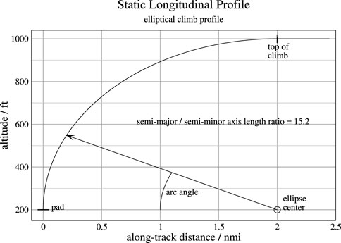
FIGURE 3. Static longitudinal profile for an elliptical climb.

The descent profile is constructed using the same algorithm that is used for the climb segment, with the same or different parameters, then it is reversed and shifted along-track to match the end with the end of the specified route. A steady level cruise segment is then inserted between the climb and descent profiles to fill the gap between them and complete the static longitudinal profile. If the route is too short for a level cruise segment at the specified altitude, then a lower cruise altitude should be used or the length of the climb and descent segments should be decreased, or both.

Each discrete point of the static longitudinal profile consists of an along-track distance and an altitude. After the power model (to be discussed later) is applied, each point will also have a time associated with it. The distance and time spacing between points can vary, and they are arbitrary within a wide range, but a few basic considerations apply. The smaller the spacing between points, the higher the resolution of the trajectory will be (and the more computation and storage space will be required, of course). Numerical roundoff error can become significant if the time steps are too small, but with standard 64-bit floating-point arithmetic they would have to be very small for that to become a concern. A more detailed description of the construction of the static longitudinal profile now follows.

For an ellipse centered at the origin and aligned with the x and y coordinate axes, the position at any given angle θ is x = a sin θ and y = b sin θ where a and b are the semi-major and semi-minor axes of the ellipse. As shown in Figure 3, the ellipse is not centered at the origin in this case but is tangent to the vertical axis at the pad elevation (or at the top of the vertical climb segment if there is one), so appropriate offsets are required. The semi-minor axis in this case is the height of the ellipse from the pad (or the top of the vertical climb segment) to the cruise altitude. The semi-major axis is the along-track distance in climb from takeoff to cruise altitude. The axis scales in Figure 3 are very different, so the actual shape of the ellipse is distorted as shown, having a semi-major (horizontal) to semi-minor (vertical) axes length ratio of 15.2.

A function was needed to map from the arc distance along the ellipse to the along-track and altitude coordinates of the point at that distance. A closed-form equation for that mapping is not possible, unfortunately, but a precise numerical mapping was constructed by sweeping the angle through the full range from zero to 90 deg in small angular increments and constructing an interpolated mapping from the integrated arc distance to the along-track distance and altitude. The size of the angular increment should be small enough for high resolution but not so small that numerical roundoff error becomes an issue. That covers a wide range, and a value of deg/8 was arbitrarily selected. The details will not be presented here, but the resulting function was used to step through the arc distance in small increments to construct the static longitudinal profile as will now be explained.

As mentioned earlier, the distance between points can vary and is arbitrary within a wide range. The distance spacing is perhaps not as critical as the time spacing, but the time spacing is not known until the power function (to be presented later) is applied. Hence, determining reasonable distance steps requires a manual iteration process: distance steps are selected, and if the resulting time steps are too large, smaller distance steps are tried, and the procedure is repeated until the time steps are within the desired range. Note that this manual iteration is only required once for each power model and static longitudinal profile, not for every trajectory. Moreover, a new iteration is unlikely to be needed even for a new profile unless it is dramatically different than the one for which the iteration was already done. For the purposes of this paper, time steps in the range of approximately 0.1 s to 1.0 s are considered reasonable, with smaller time steps preferred in the dynamic segments and larger in steady-state. The power of modern computers allows for high resolution at a negligible cost in terms of both computation time and data storage.

For the initial vertical climb segment, the vertical speeds are low, so small step sizes in arc distance are needed. Actually, several different step sizes were needed, ranging is size from 0.125 ft at takeoff and increasing to 2 ft at an arc distance of 600 ft. After that point, the speed is higher, and an increment of 10 ft was used. When the power model described in the next subsection was applied, these arc distance step sizes yielded the desired range of time steps.

3.1.1 Altitude change maneuvers

A key type of maneuver for conflict resolution is altitude change, usually from flying level at one altitude to flying level at another. Figure 4 shows an example of such an altitude transition in level flight from 1,000 to 1,500 ft. These maneuvers must be smooth enough for passenger comfort, and they must also be completed within a given distance to avoid the conflict. For imminent conflicts, the distance takes precedence over passenger comfort.

FIGURE 4

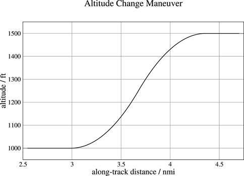
FIGURE 4. Example altitude change maneuver profile.

The algorithm used here for this type of maneuver works as follows. The flightpath (climb or descent) angle is incremented in small angular increments (a value of deg/8 was used in the example) at a constant rate from zero to a specified maximum magnitude, which can be in the range of approximately 5–20 deg. A value of 10 deg was used for the example. The rate of increase of the flightpath angle is a constant parameter that should normally be in the range from approximately 5–30 deg/nmi, depending on the traffic situation and the distance to the conflict to be resolved. A value of 10 deg/nmi was used for the example, resulting in a total maneuver length of 1.33 nmi.

The normal (vertical) acceleration for this kind of maneuver is approximately a_n = rs², where s is the speed and r is the rate of increase of the flightpath angle. The value of 10 deg/nmi that was used for the example shown in Figure 4 yields a normal acceleration of 0.043 g, which is mild and acceptable for passenger comfort. The threshold for passenger comfort is approximately 0.1 g, but a lower value of approximately 0.05 g is preferable if the traffic situation allows it. Another way to select a value for this rate is to start with a desired value for normal acceleration and compute the required rate of increase of flightpath angle as r = a_n/s². For example, the required rate for a normal acceleration of 0.05 g and a speed of 130 knots is 11.6 deg/nmi.

The algorithm starts by constructing the profile to the center altitude, half way between the initial and final altitudes. To realize symmetry, that first half of the profile is then reflected, first vertically about the center altitude, then horizontally about the end point, to form the second half of the profile. The two-halves of the profile meet in the center at a flightpath angle that was limited to a maximum magnitude of 10 deg in the example shown in Figure 4. However, that value was never reached in the example, where the actual maximum flightpath angle was 6.9 deg. Whether the maximum allowed magnitude of the flightpath angle is reached or not depends on the parameters of the maneuver.

3.2 Power model and longitudinal profile

As mentioned earlier, a longitudinal profile consists of 1) the horizontal distance flown as a function of time and 2) the altitude as a function of time or distance. It is essentially the resulting trajectory with the route “bent” into a straight line, assuming decoupled lateral and longitudinal dynamics. It will be constructed here for air taxis by assigning time as a function of arc distance to the static longitudinal profile constructed above. In other words, a time will be computed as follows to yield a specified net power for each discrete point of the static longitudinal profile.

Also as mentioned earlier, the net power at any time is not necessarily based on the maximum power available at the current flight state. It cannot exceed the maximum power available, of course, and it should leave a margin for controllability. The maximum power available, and hence the maximum net power available at any time, depends mainly on the airspeed (CAS) at that time, but the net power function is essentially a control variable that can be programmed as a function of any flight variable, including time, position along the route, altitude, and flightpath angle. For purposes of this paper, it will be modeled as a function of CAS only.

As mentioned in the Introduction, the methods used in this paper are based in part on the Trajectory Specification concept (Paielli, 2022), which allows the time steps of the reference trajectory to vary in size, typically being larger in steady-state flight than otherwise. That allowance for varying time steps is used here to set the power level by computing the time step between discrete points in 3D space that yields the specified power at that time. The TS software then automatically converts the time steps to a specified uniform time step by linearly interpolating between the varying time steps.

Once the interpolated points with equal time steps are computed, any relevant flight variable as a function of time or along-track distance can be precomputed as an array with uniform time or distance steps for fast lookup. If the start time of the trajectory is t₀, and the time step is Δt, then the array index corresponding to time t is simply (t − t₀)/Δt. Because that index value is usually not an exact integer, the values of the array at the two closest bounding integer indices are linearly interpolated for better accuracy. This procedure provides a fast (constant-time) lookup and interpolation of the relevant flight variables as a function of time or distance, making the trajectory model effectively continuous in time and space.

Total mechanical energy is the sum of potential and kinetic energy:

$E=mgh+m{v}^2/2(1)$

where m is the vehicle mass, g is gravitational acceleration, h is altitude, and v is velocity (speed). (This energy does not include the rotational kinetic energy in the rotors, which is not relevant here.) Now consider the change in the total energy over a single discrete time step of length Δt. The average power over that time step is P = ΔE/Δt, so

$P\mathrm{\Delta }t=\mathrm{\Delta }E=mg\mathrm{\Delta }h+m\mathrm{\Delta }\left(v^2/2\right)=mg\mathrm{\Delta }h+m{v}_1^2/2-m{v}_0^2/2(2)$

where v₀ and v₁ and the speeds are the start and end of the interval. The average speed over the time interval is v = Δd/Δt, where d is the arc distance flown over the interval (the hypotenuse of the horizontal and vertical distance between points). Substituting this expression for v₁ yields

$P\mathrm{\Delta }t/m=g\mathrm{\Delta }h+{\left(\mathrm{\Delta }d/\mathrm{\Delta }t\right)}^2/2-v_0^2/2(3)$

Multiplying both sides by (Δt)² and rearranging yields

$P{\left(\mathrm{\Delta }t\right)}^3/m+\left(v_0^2/2-g\mathrm{\Delta }h\right){\left(\mathrm{\Delta }t\right)}^2-{\left(\mathrm{\Delta }d\right)}^2/2=0(4)$

This is a cubic polynomial of the form ax³ + bx² + cx + d = 0 where x = Δt and

$a=P/m(5)$

$b=v_0^2/2-g\mathrm{\Delta }h(6)$

$c=0(7)$

$d=-{\left(\mathrm{\Delta }d\right)}^2/2(8)$

This cubic polynomial equation can be solved using the formula given in the Appendix A to determine the time increment between points to yield a given level of net power in excess of the power needed to maintain steady level flight at the current airspeed and altitude. There should be only one positive real root, which will be the correct solution. Given a sequence of position points in 3D space, plugging in the desired power per unit mass and the other relevant variables into the equation allows the required time difference between points to be determined.

Determining the power model from simulated or recorded data can be done as follows. The trajectory should be given in terms of a closely spaced series of points in 4D space. That series can be effectively differentiated with respect to time by back-differencing to determine velocity, and the velocity and altitude at each point can then be used to determine total mechanical energy according to Eq. 1. Net power is then the time derivative of energy at each point. CAS can be computed at each point, based on standard equations, as a function of speed, altitude, and the wind vector, if applicable. Note that CAS and net power must be determined separately for climb and descent. Once they are determined, the resulting CAS-power points can be ordered by CAS value and interpolated to make the CAS steps uniform for efficient (constant-time) array access followed by linear interpolation (as discussed earlier for time steps). If the resulting function is not smooth enough, a smoothing algorithm or a curve fit (e.g., polynomial) can be used to make it smoother.

Figure 5 shows the net power vs. CAS for the QEP1 (Shaw-Lecerf et al., 2020), a Quadrotor Electric Power single-seat aircraft. The QEP1 has a rotor diameter of 12.62 ft and an operating gross weight of 1,428 pounds. The dashed red line is the model target function to be emulated, which is derived from simulated trajectory data in the form of a sequence of data points in 4D space (t,x,y,z) with a uniform time step of 1.0 s. The solid black line (which obscures much of the red line) represents the resulting net power function, which matches the model very closely, verifying the correctness of the cubic polynomial solution presented above. The slight discrepancies are due to discretization error. The descent was modeled as the negative mirror image of this function but is not shown. The net power at takeoff is approximately 300 fpm, and the maximum power is approximately 1,300 fpm at a CAS of approximately 85 knots.

FIGURE 5

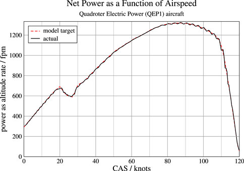
FIGURE 5. Example of net power as a function of calibrated airspeed (CAS).

It is worth noting that the power models discussed in this paper are actually models of power/weight ratio. They should therefore be scaled by the inverse of the weight if the weight of the aircraft differs significantly from what it was when the trajectory data that the power model is based on was generated. In practice, a weight estimate could be based on the number of passengers (as is currently done for airliners). The weight could also serve as a proxy for the available battery power. If the batteries are not fully charged, the assigned weight could be arbitrarily increased by the ratio of the nominal battery power to the current reduced battery power.

Figure 6 shows the climb profile that results from applying the power algorithm to the static longitudinal profile shown in Figure 3 above. The top plot shows altitude as a function of time, and the bottom plot shows speed as a function of time, where the steady cruise speed is 122 knots. The descent profile is essentially the mirror image of this profile. The resulting time steps are in the desired range from 0.1 s to 1.0 s as discussed earlier. The black vertical line marks the top of climb and the start of level flight, and the small red vertical line marks the point at which the steady cruise speed is reached.

FIGURE 6

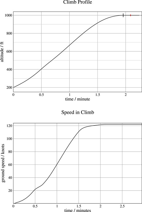
FIGURE 6. Top: Climb profile, for example, trajectory; bottom: speed.

Figure 7 shows the resulting energy and power profiles. The top plot shows the potential, kinetic, and total mechanical energy as a function of time (excluding the rotational kinetic energy in the rotors), where energy is represented as altitude equivalent (energy per unit mass divided by gravitational acceleration). The point at which a steady altitude is reached is marked on the potential energy (altitude) curve, and the point at which steady speed is reached is marked on the kinetic energy curve. The point at which steady altitude and speed are both reached (i.e., the later of the two points) is marked on the total energy curve. The symmetry is due to the symmetric modeling of climb and descent power in this example.

FIGURE 7

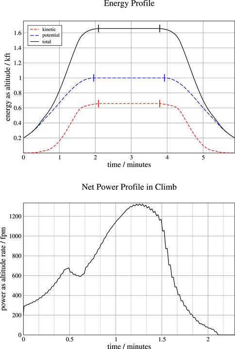
FIGURE 7. Top: total mechanical energy profile in climb for example trajectory; Bottom: power profile in climb for example trajectory.

The bottom plot Figure 7 shows the resulting power profile as a function of time during climb. As explained earlier, this power is the rate of change of the mechanical energy and is represented here as altitude rate or vertical speed equivalent (power per unit mass divided by gravitational acceleration). The power drops to zero when steady-state flight at the cruise speed and altitude is reached. The net power in descent is the negative mirror image of this plot but is not shown here.

3.3 Mapping to a route

A route is the vertical projection of a trajectory onto the geodetic surface of the earth. In the Trajectory Specification (TS) concept (Paielli, 2022), a route is specified as a sequence of waypoints on that surface and a turn radius associated with each waypoint. The TS algorithm takes those route parameters and constructs a detailed route representation consisting of alternating straight and turn segments. All turns are tangent-arc or “flyby” turns of constant radius. If two successive waypoints are too close together for the specified turn radius, the route is geometrically invalid and is flagged as such by the TS software (but is left for the user to correct by changing either the radius or the waypoints). The route representation constitutes a curvilinear coordinate system in which the coordinates are along-track distance and cross-track position, which can be converted to geodetic or locally level Cartesian coordinates and vice versa.

Recall that the static longitudinal profile was adjusted to the path length of the specified route by adding a steady cruise segment of the required length between the climb and descent segments. Applying power to determine the time values does not change the length of the longitudinal profile, so it will still have the same length as the specified route. It is then superimposed onto the route by mapping the along-track distance of each discrete point onto the corresponding position at that distance on the route (assuming no cross-track error). This has the effect of “bending” the straight longitudinal profile onto the route, assuming decoupled lateral and longitudinal dynamics as before.

As mentioned earlier, the simplifying assumption of decoupled lateral and longitudinal dynamics can be inaccurate, particularly for large turns at high bank angles during climb. The bank angle for a coordinated turn is ϕ = atan(v²/(rg)), where v is speed, r is the turn radius, and g is gravitational acceleration. The component of net power that is in the longitudinal plane is the overall net power scaled by cos ϕ, the cosine of the bank angle. For a bank angle of 20 deg, for example, the longitudinal component is 6.0% less than the overall net power. If the overall net power can be increased by a factor of 1/(cos ϕ), the effect can be offset, and the assumption of decoupled lateral and longitudinal dynamics will be valid. For a bank angle of 20 deg, that requires a 6.4% increase in net power. If power cannot be increased that much, which typically happens only in climb, then the net power model can be adjusted to account for the diminished longitudinal power during the turn.

3.4 Modeling the effect of winds

A wind model is usually not required for ATC simulation unless the fidelity of the simulation is intended to be high. To actually use this method of trajectory generation in the field, however, the current winds must be accounted for because the power required in flight depends on the winds. In a cross-wind, the aircraft needs extra power just to stay on course, which is another reason that a margin should be maintained away from maximum power. On the other hand, a headwind or tailwind determines the groundspeed at a given airspeed and vice versa. The cross-wind effect is more subtle and will not be addressed here, but the effect of the along-track wind component (headwind or tailwind) can be modeled as follows.

If a simulated trajectory is used to determine the power model, it should be simulated with zero winds, and if a recorded trajectory is used, it should preferably be recorded in low-wind conditions. After the new trajectory is generated and mapped to a route as explained earlier, the effect of the current wind field during level flight can be modeled by adjusting groundspeed for the headwind or tailwind at each point along the route. This method is equivalent to adjusting the along-track position by the integrated along-track component of the wind vector along the route.

Nonlevel flight segments can be modified similarly, except that the adjustment in along-track position should be scaled by the cosine of the flightpath angle (relative to horizontal) at any given point. Hence there would be no adjustment in a vertical segment, and the adjustment in a level segment would be as discussed above. This method preserves the static path of the trajectory in 3D space while accounting for the main wind effects in terms of progress in time along the route.

4 Flight time dependence on parameters

The utility and economic viability of Urban Air Mobility will depend on how much time can it can save compared to driving, so it is interesting to analyze how various trajectory parameters affect trip flight times.

The top plot of Figure 8 shows how the flight time varies as a function of the cruise altitude, with climb distance (from takeoff to top of climb, the semi-major axis of the ellipse) as a parameter, for a route of 20 nmi, using the same power model that was used in the earlier examples. The dependence is significant, with flight time increasing by 3.6 min as cruise altitude is increased from 1.0 to 2.0 kft with a climb distance of 2 nmi. The time increases by another 4.7 min as cruise altitude is increased again from 2.0 to 3.0 kft, and another 5.4 min from 3.0 to 4.0 kft, for a total increase of 13.6 min as cruise altitude is increased all the way from 1.0 to 4.0 kft. The increases in trip flight time with altitude are even larger for a smaller climb distance of 1.0 nmi. This plot clearly shows the time advantage of staying at lower altitudes and the economic disincentive of flying in the upper regions of the UAM airspace for this particular aircraft model at least, which may be somewhat underpowered. At some point, the time advantage over driving is lost (and the travel time to and from the vertiports must also be accounted for, of course).

FIGURE 8

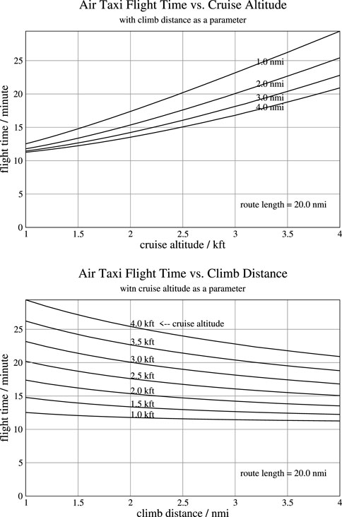
FIGURE 8. Top: Flight time as a function of cruise altitude; Bottom: Flight time as a function of climb distance.

The bottom plot of Figure 8 shows how total flight time varies as a function of the climb distance, with cruise altitude as a parameter, for the same vehicle as the top plot. At a cruise altitude of 1,000 ft, the trip flight time decreases by 0.7 min as the climb distance is increased from 1.0 to 2.0 nmi, and it decreases by 1.3 min as the climb distance is increased from 1.0 to 4.0 nmi. The time reductions are larger at higher cruise altitudes. According to this plot, shallower climbs reduce flight time, and the climb distance should be maximized to minimize flight time. The same applies for the descent distance, so the shortest flight time requires the climb and descent to meet somewhere in the middle, with no level cruise segment. However, that could reduce airspace capacity by blocking altitudes that other flights need, so it cannot always be done and perhaps should rarely be done. Further analysis is required to determine the best values to use for climb and descent distance based on the traffic scenario.

Figure 9 shows flight time as a function of power, with cruise altitude as a parameter, for a climb distance of 2.0 nmi. As before, power is expressed as power per unit mass divided by gravitational acceleration, in units of fpm. The power level is varied as a scale factor of the climb power shown in Figure 5, where a power factor of 1.0 corresponds to that same power function. The negative power level in descent was left unchanged because it does not depend on available power. Because power is actually power per unit mass, the power factor can also be considered the inverse of a scale factor on aircraft mass or weight.

FIGURE 9

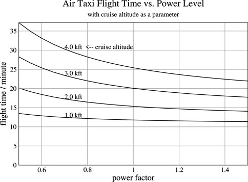
FIGURE 9. Flight time as a function of power level.

Figure 9 shows that flight time can be sensitive to power level, perhaps even more sensitive than it is to speed for shorter flights. In particular, decreased power levels can significantly increase trip flight time at the higher cruise altitudes. At the lowest shown cruise altitude of 1,000 ft, however, the sensitivity to power level is minimal over a wide range. Also, the sensitivity increases with cruise altitude and decreases as power/weight ratio increases. And because power per unit mass depends on weight, the flight time can also be sensitive to the payload mass, hence more passengers can mean significantly longer flight time, particularly for smaller aircraft at higher cruise altitude. Underpowered aircraft could hamper the UAM business model with flight times that offer no significant time savings over driving.

5 Conclusion

A new method has been developed to generate flyable trajectories for eVTOL urban air taxis. The method allows the user to directly specify the route, the static longitudinal profile, and a power model as a function of airspeed (CAS) and possibly other flight variables. This method has the advantage over previous methods of not requiring a detailed aircraft model or a model of the flight controls.

The trajectory generation algorithm is composed of four main parts: 1) generating the static longitudinal profile, 2) converting it to a (dynamic) longitudinal profile by applying a power model, 3) superimposing that profile onto a specified route, and 4) adjusting for the effects of winds.

A novel method was developed to yield the specified power model as a function of airspeed by solving a cubic polynomial for the required time step between discrete points in the longitudinal plane.

Because the climb trajectory starts vertically and ends horizontally, an elliptical profile (a quarter of an ellipse) was used as an example profile shape, which is smoother than other profiles that have been proposed.

The dependence of trip flight time on various parameters was analyzed and plotted, showing that flight times are significantly longer for higher cruising altitudes, steeper climbs, and lower power levels. These dependencies have implications for the economic viability of UAM as an alternative to driving.

This method can be used to generate candidate trajectories for conflict resolution, which can then be checked to find the candidate with the shortest flight time that is free of conflicts. Using advanced feedforward/feedback control methods, aircraft should be able to fly the resulting deconflicted trajectories to within specified tolerances in the field.

Data availability statement

The raw data supporting the conclusions of this article will be made available by the authors, without undue reservation.

Author contributions

RP: Conceptualization, Methodology, Software, Writing–original draft.

Funding

The author(s) declare that no financial support was received for the research, authorship, and/or publication of this article.

Acknowledgments

The author acknowledges and thanks Chris Silva of NASA Ames Research Center for running the NDARC (Johnson, 2015) program to provide the rate-of-climb data that is plotted in Figure 2.

Conflict of interest

The author declares that the research was conducted in the absence of any commercial or financial relationships that could be construed as a potential conflict of interest.

Publisher’s note

All claims expressed in this article are solely those of the authors and do not necessarily represent those of their affiliated organizations, or those of the publisher, the editors and the reviewers. Any product that may be evaluated in this article, or claim that may be made by its manufacturer, is not guaranteed or endorsed by the publisher.

References

Chatterji, G. (2020). “Trajectory Simulation for Air Traffic Management Employing a Multirotor Urban Air Mobility Aircraft Model,” in 2020 AIAA aviation forum (AIAA (American Institute of Aeronautics and Astronautics)).

CrossRef Full Text | Google Scholar

Cubic equation (2001). Wikipedia. Avaliable at: https://en.wikipedia.org/wiki/Cubic_equation#General_cubic_formula.

Google Scholar

Goodrich, K. H., and Theodore, C. R. (2021). “Description of the NASA Urban Air Mobility Maturity Level (UML) Scale,” in AIAA scitech 2021 forum (USA: AIAA).

CrossRef Full Text | Google Scholar

Hill, B. P., DeCarme, D., Metcalfe, M., Griffin, C., Wiggins, S., Metts, C., et al. (2021). UAM vision concept of operations (ConOps) UAM maturity level (UML) 4,” version 1.0, prepared. NASA.

Google Scholar

Johnson, W. (2015). Ndarc: NASA design and analysis of Rotorcraft. NASA Technical Paper 2015-218751.

Google Scholar

Paielli, R. A., and Erzberger, H. (2019). Trajectory Specification for Terminal Airspace: conflict Detection and Resolution. AIAA J. Air Transp. 27 (2), 51–60. doi:10.2514/1.D0132

CrossRef Full Text | Google Scholar

Paielli, R. A. (2022). Trajectory specification applied to terminal airspace. NASA Technical Paper NASA/TP-20220000348.

Google Scholar

Shaw-Lecerf, M., Ingram, C., Gu, F., and Chung, W. (2020). “Developing Urban Air Mobility Vehicle Models to Support Air Traffic Management Concept Development,” in AIAA aviation 2020 forum (AIAA). doi:10.2514/6.2020-3191

CrossRef Full Text | Google Scholar

Silva, C., Johnson, W., Antcliff, K. R., and Patterson, M. D. (2018). “VTOL Urban Air Mobility Concept Vehicles for Technology Development in 2018 aviation technology, integration, and operations conference, AIAA aviation forum (Dallas, TX: AIAA 2018-3847).

CrossRef Full Text | Google Scholar

Takahashi, M. D., Whalley, M. S., Mansur, H., Ott, C. R., Minor, J. S., Morford, Z. G., et al. (2017). Autonomous Rotorcraft Flight Control with Multilevel Pilot Interaction in Hover and Forward Flight. J. Am. Helicopter Soc. 62, 1–13. doi:10.4050/jahs.62.032009

PubMed Abstract | CrossRef Full Text | Google Scholar

Thipphavong, D. P., Apaza, R. D., Barmore, B. E., Battiste, V., Belcastro, C. M., Burian, B. K., et al. (2018). Urban Air Mobility Airspace Integration Concepts and Considerations in AIAA aviation (The MITRE Corporation).

Google Scholar

Urban Air Mobility (UAM) (2020). NextGen urban air mobility (UAM) concept of operations. Federal Aviation Administration, Version 1.0.

Google Scholar

Zhang, Y., Satapathy, G., Manikonda, V., and Nigam, N. (2010). KTG: A Fast-time Kinematic Trajectory Generator for Modeling and Simulation of ATM Automation Concepts and NAS-wide System Level Analysis in AIAA modeling and simulation technologies conf (Toronto, Ontario Canada: AIAA). doi:10.2514/6.2010-8365

CrossRef Full Text | Google Scholar

Appendix A: Cubic polynomial roots

A cubic polynomial of the form

$a{x}^3+b{x}^2+cx+d=0(9)$

where a ≠ 0, can be solved using complex mathematics as follows (from Wikipedia (Cubic equation, 2001)). First, the following terms are defined.

$d_0\equiv b^2-3ac(10)$

$d_1\equiv 2b^3-9abc+27a^{2}d(11)$

$z\equiv \sqrt{d_1^2-4d_0^3}(12)$

$f\equiv d_1+z(13)$

$h\equiv \text{\hspace{0.17em}if\hspace{0.17em}}f\ne 0\text{\hspace{0.17em}then\hspace{0.17em}}f\text{\hspace{0.17em}else\hspace{0.17em}}{d}_1-z(14)$

$g\equiv \left(\sqrt{-3}-1\right)/2(15)$

$C_1\equiv \sqrt[3]{h/2}(16)$

$C_2\equiv g{C}_1(17)$

$C_3\equiv g{C}_2(18)$

The three roots for x are then

$x_i=-\left(b+C_i+d_0/C_i\right)/\left(3a\right),i=\mathrm{1,2,3}(19)$

At least one root must be real, and the other two can be either real or complex. However, a real root can be computed to have a tiny imaginary part due to numerical roundoff error, so the root that has the smallest imaginary magnitude should have its imaginary part set to zero and be taken as a real root.