Model-based manoeuvre analysis: a path to a new paradigm in aircraft flight dynamics

1 List of symbols

The list of symbols used in this article is given in Table 1 below.

TABLE 1

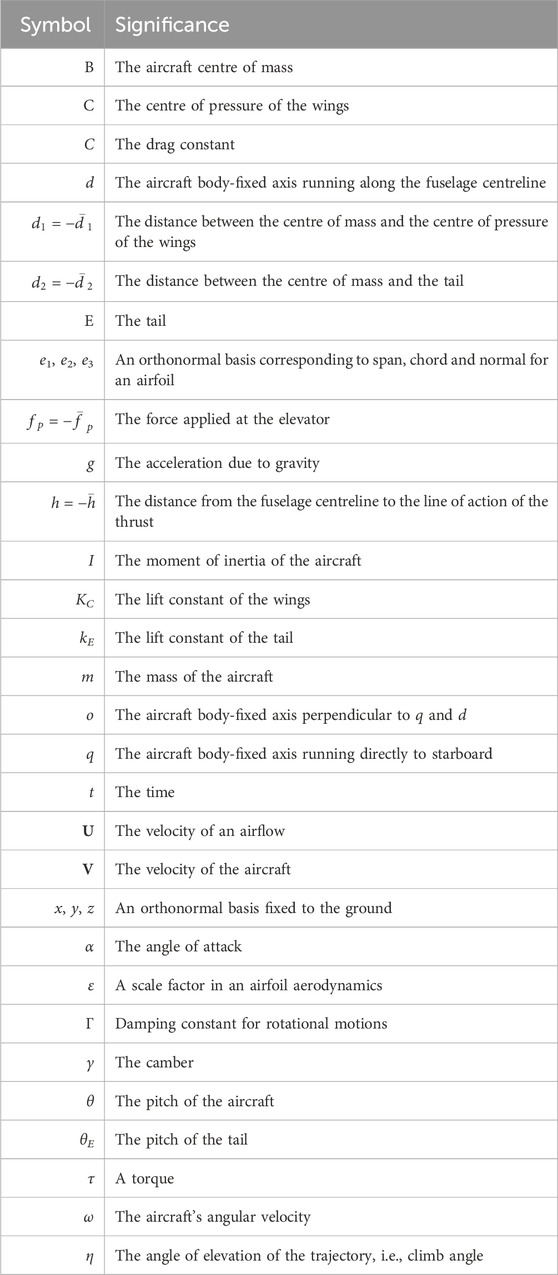
TABLE 1. List of symbols used in this article.

2 Introduction

The dynamics of aircraft flight is a subject which is of relevance to two classes of technical audiences—university students and teachers, and pilots and flight instructors. Currently, this subject is presented to these two audiences in completely disparate ways.

If we look at a sample of academic textbooks on flight dynamics (Etkin, 1971; Nelson, 1998; Phillips, 2004; How, 2004; Caughey, 2011), we find that the greatest emphasis by far is on the normal modes of an aircraft—short period, phugoid, spiral, roll subsidence and Dutch roll—and their stabilities. This material (or a subset thereof if primarily pitch plane motions are focused on) is present in almost every instance. The rationale behind this topic selection has been excellently explained by George Bryan, whose seminal work (Bryan, 1911) in 1911 opened the field of academic flight dynamics: “In reading the accounts of accidents, both fatal and otherwise, that appear every few days in the daily papers, it is difficult to avoid coming to the conclusion that much of this loss of life and damage could be avoided by a systematic study of stability and certain other problems regarding the motion of airplanes particularized in this book.” The technique as well as philosophy behind the approach to academic flight dynamics has seen little change during the 110 years since Bryan’s groundbreaking work. Modern textbooks with a more applied flavour (Anderson, 1989; Pamadi, 1998; Saarlas, 2007), such as books on aircraft performance, supplement the stability calculations with discussions of runway length, thrust or braking force required during takeoff and landing runs, climb performance and range optimization considerations. Only rarely do we see instances of actual flight simulations entering the curriculum; one example where this does happen is in Sinha and Ananthkrishnan (2014). Here too the simulations, demonstrated for a modified FA18 fighter jet, are pretty basic, mostly covering the response of the aircraft to step changes in thrust, elevator deflection and other control inputs.

Literature on the theory of piloting begins with Wolfgang Langewiesche’s pioneering 1944 work (Langewiesche, 1944). To quote him, “What is wrong with the theory of flight ..... is that it is the theory of the wrong thing—it usually becomes a theory of building the airplane rather than of flying it. [This theory] neglects those phases of flight that interest the pilot most.” The theory that Langewiesche was referring to was Bryan's theory of stability, which explains his comment. Langewiesche presents his own intuitive and entirely qualitative treatment of flight dynamics, going as far as one can go without taking recourse to mathematical equations. The content of his book appears essentially invariant in similar works upto the present (Hurt, 1959; Barnard and Philpott, 2010; CAE Oxford Aviation Academy, 2014; Badick and Johnson, 2022). The reduced dependence on mathematics here sometimes restricts the scope of the treatment. We shall see examples of this in the present article.

It is natural to wonder, if the runway length during landing can be calculated in detail, then why cannot the same hold true for the approach and flaring technique. Perhaps this is because runway lengths are obtained from explicit equations of motion (Newton’s laws with thrust, drag and friction) while full-scale flight manoeuvres such as flaring are not. Beginning with Bryan’s work, all current equations for aircraft motion use coefficients of lift, drag and elevator moment, denoted C_L, C_D and C_m, which are unspecified functions of the speed, angle of attack and other variables. These functions exist only as data tables, obtained from experiments and/or computational fluid dynamics (CFD) simulations. Given these tables, two approaches are commonly used. The first, propounded by Bryan himself, is to work in terms of linearized equations, valid near the linearization point. The second approach is to use nonlinear equations. This requires one to construct C_L, C_D and C_m by interpolation from the data tables, with linear, cubic or higher-order polynomial interpolants being typical. Some examples of studies using such an approach are Refs. (Jahnke, 1990; Guicheteau, 1998; Lowenberg and Champneys, 1998; Macmillen, 1998; Hassan and Taha, 2017; Rohith and Sinha, 2020).

The only explicit equation till date for a flying vehicle is the model derived independently by Lanchester (Lanchester, 1908) and Zhukovsky (Zhukovsky, 1949) for a glider (unpowered aircraft):

$\frac{\mathrm{d}V}{\mathrm{d}t}=-a{V}^2-\sin \eta (\mathrm{1a})$

$\frac{\mathrm{d}\eta }{\mathrm{d}t}=\frac{V^2-\cos \eta }{V},(\mathrm{1b})$

where V denotes the speed of the glider and η denotes the angle which the flight path makes with the horizontal. The system Eq. 1a, b ignores the aircraft’s pitch as a separate variable. Since the pilot uses pitch control to regulate the flight path of a real aircraft, be it powered or unpowered, this makes Eq. 1a, b simplified to the point of being divorced from reality. Stengel (2004) presents an instance where Eq. 1a, b is used to analyse the dynamics of a paper plane; even so, the author acknowledges the limitations to the analysis arising from the absence of pitch.

While aircraft manoeuvres have not entered the mainstream flight dynamics curriculum so far, we would be remiss if we do not mention a few research articles which touch upon the issue. In these studies, given the aircraft dynamic model and the desired trajectory, the technique of inverse simulation (Hess et al., 1991) has been used to obtain the control inputs which must go into generating the trajectory. Examples include barrel roll in an F4 fighter jet (Hess et al., 1991), a helicopter flying a slalom (Thomson and Bradley, 2006) and an unmanned air vehicle (UAV) performing different manoeuvres (Murray-Smith and Mcgookin, 2015). A more theoretical treatment can be found in Krishchenko et al. (2009) which incidentally uses a slightly modified version of Eq. 1a, b as the underlying model. Modelling of human pilots can also be found in Padfield (2011); Lone and Cooke (2014), the first using τ-theory and the second using transfer functions modelling various aspects of a human pilot such as perception and neuromuscular reaction. We are yet to realize the full impact of these works on either academic or operational flight dynamics.

In this article, we show the beginnings of how one may bridge the gulf between theoretical flight dynamics and practical aircraft operation. To this end, we first construct a closed-form dynamic model of the aircraft. Compared to a data table model, this will help significantly because the complete tables exist in the public domain for only a handful of aircraft models, such as an F4 model (Lowenberg and Champneys, 1998), F16 model (Saetti and Horn, 2022) and FA18 model (Sinha and Ananthkrishnan, 2017). If one desires to construct a generic model not tailored to a particular aircraft, then it is difficult to figure out the generalizations and modifications which need to be made to the tables. With a closed-form model however, the unknowns are constants rather than multivariate functions. We can choose the constants to make the model represent the type of aircraft we want, for instance a passenger airliner, a piston-engine trainer or a stealth fighter. An explicit equation will enable full flight manoeuvres to attain the same status as considerations like runway length, climb gradient and range. Closed-form equations also enable a large range of nonlinear dynamical techniques to be brought to bear on the problem, which data-centric equations do not. We shall see this later on in the article.

To construct the model, we recognize that although the fundamental origins of lift and drag on an aerodynamic body immersed in an airflow are still subject to debate (Regis, 2020; Gonzalez and Taha, 2022; Liu, 2023), the resulting expressions for forces and torques on the body are simple (especially in the non-stall regime), and those alone are sufficient to yield the dynamics of a single aircraft flying in isolation. For simplicity, we restrict ourselves to two-dimensional motions in the pitch plane or longitudinal plane. This is where lift is generated, and many interesting manoeuvres such as takeoff and landing also take place in the pitch plane. Hence it is natural to consider this case at first. After proposing the model, we validate it by demonstrating the short period and phugoid modes as well as the regions of normal and reversed command. The successful derivation of the normal modes and their stabilities also ensures that our model passes the basic requirements of the university curriculum. We then show how the external excitations in the equations of motion—the thrust and elevator force (pilot stick input)—can be chosen to make the (model) aircraft perform different manoeuvres. Here we consider two manoeuvres, both taken from acrobatic flying. The first is the Immelmann turn while the second is the vertical dive (and recovery!). After these demonstrations, we conclude with a discussion of the implications and ramifications of our results.

3 Methods

3.1 Lift formula

To derive the closed form aircraft dynamic model, we start from the simplest mathematical expression for lift and drag on an airfoil (aircraft’s wings and tail) which agrees with experiments. Let x, y, z denote a ground-fixed dextral, orthogonal axis triplet and let e₁, e₂, e₃ be a triplet corresponding to the span, chord and normal for an airfoil. When the airfoil is mounted in an airflow U, the e₁-component of the flow does not generate lift, so we assume that the flow occurs in the e₂-e₃ plane only. Without loss of generality, we take e₁ = x and $\mathbf{U}=-U\widehat{\mathbf{y}}$ (throughout this article, hat denotes unit vector); we rotate the airfoil about the e₁-axis to achieve different flow geometries. Let the axes e₂ and e₃ make an angle of attack α with y and z. We can see the geometry in Figure 1.

FIGURE 1

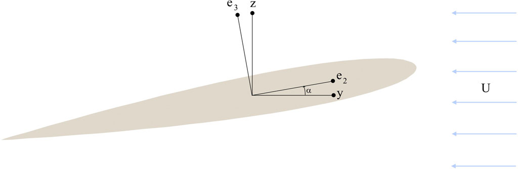
FIGURE 1. The airfoil showing the relevant axes and angles. U represents the airflow in a reference frame where the airfoil is stationary.

Now, define a scale factor ɛ and the camber γ such that when the airfoil’s true angle of attack is α, its effective angle of attack is

${\alpha }^{\prime }=\epsilon \left(\alpha +\gamma \right)(2)$

Here, ɛ is of order unity while camber γ, when non-zero, is typically a few degrees. Let $e_2^{\prime }$ and $e_3^{\prime }$ denote axes rotated through α′ relative to y and z. Then, our formula for the aerodynamic force on the airfoil is

$\mathbf{F}=-K{U}_{e_2^{\prime }}{U}_{e_3^{\prime }}{{\widehat{\mathbf{e}}}^{\prime }}_3(3)$

where K is a constant which we call the “lift constant”. The expression (Eq. 3) has the following features (note that in the ‘base case’ of ɛ = 1 and γ = 0, α′ = α):

• The magnitude of the lift F_L (component of F normal to U) is KU² sin α′ cos²α′. Practically, α′ must be small for the airfoil not to stall. In this case, the lift is proportional to U² and α′, both of which agree with experiments. If K is made proportional to the density ρ of the air, then that dependence agrees with experiment also.

• F also has an induced drag F_D (component of F parallel to U) with the value F_L tan α′. Induced drag directly proportional to the lift is a hallmark of all real airfoils. The lift-to-drag ratio (L/D) is cot α′. Decreasing L/D with increasing angle of attack is observed in experiments (Webb et al., 2001; Noronha and Krishna, 2021), beyond the smallest α′s where parasitic drag dominates. For a given airfoil, the parameter ɛ controls L/D at a particular α.

• Eq. 3 is a quadratic polynomial in velocity components, which results in analytical simplicity of all equations derived on its basis.Note that K, ɛ and γ are constant if the air density is constant and the wing geometry i.e., flap setting does not change, all of which hold true for typical flight manoeuvres. The distribution of F over the surface of the airfoil determines the torque exerted on it. The torque is equivalent to the entire force acting through one point called the centre of pressure (CP). For our purposes it will be sufficient to treat the location of CP as a given.

Since we shall be performing the stability analysis and demonstrating the manoeuvre simulations for a hypothetical aircraft rather than an actual one, let us take γ = 0 and ɛ = 1 for the remainder of this article so that α′ = α and ${\widehat{\mathbf{e}}}_{\mathrm{2,3}}^{\prime }={\widehat{\mathbf{e}}}_{\mathrm{2,3}}$. This assumption results in a minimal model, and also makes the geometry easier to visualize while not discarding any physical phenomena. In addition to lift on an airfoil, we shall also need a formula for the parasitic drag acting on the fuselage and wings. We use the standard formula

${\mathbf{F}}_D=C{U}^2\widehat{\mathbf{U}}(4)$

where C, like K in Eq. 3, is a constant that factors in the density of air, the dimensions of the body and other quantities unrelated to the flow geometry. Before proceeding further, we again note that Eqs 3, 4 are phenomenological in origin, and make no reference to the flow field surrounding the aircraft. For this reason, our model is applicable only to a single aircraft flying in isolation, and not to aircraft flying close together, such as in formations. Civilian aviation however features with overwhelming preponderance the former case.

3.2 Geometrical features, elevator model

For the derivation of the equation of motion, we assume that the air is still (i.e., there is no wind) and that the aircraft is not in a stall. The point B is the centre of mass (CM) of the aircraft, C the CP of the wings and E the tail (assumed small enough to be treated as a point). Let the ground-frame axes be x, y, z with z vertically upwards. With origin at B, let the aircraft’s direct axis d run along the fuselage from tail to nose, quadrature axis q point directly to starboard and orthogonal axis o be perpendicular to these two, so that q, d, o form a triplet. Let q, d, o be coincident with x, y, z when all orientation angles are zero. As already mentioned, all our work in this article is in the pitch plane (y-z plane or d-o plane) alone. We assume that C and E are both located on the d-axis, with C behind B (as conventional for an aircraft) and E of course behind C. Let V be the velocity vector of B and η the angle of elevation of V, i.e., $\eta =\arctan \left(V_z/V_y\right)$. Let θ be the pitch. Assuming the wings’ e₂-axis to be parallel to the fuselage d-axis, θ − η becomes α, the angle of attack. Let m be the aircraft mass, d₁ the length BC and d₂ the length BE. Let h be the distance from the d-axis to the centreline of the engines. Let us also define ${\bar{d}}_1$ to be −d₁, ${\bar{d}}_2$ to be −d₂ and $\bar{h}$ to be −h, so that the barred quantities are positive. Let K_C be the lift constant of the wings and k_E be that of the horizontal tail; let C be the drag constant of the fuselage. The geometrical features are shown in Figure 2.

FIGURE 2

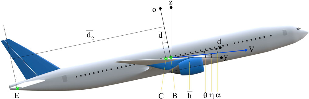
FIGURE 2. The aircraft showing axes, angles and dimensions. The q-axis comes out of the plane of the page.

We recognize that the axis nomenclature and conventions defined above differ from most Literature items which have x forward, y to starboard and z vertically downwards. Moreover, these works do not use descriptive names (such as direct, quadrature, or orthogonal) for the body axes. Our rationale for choosing a different axis convention is that in aviation, altitude is measured positive upwards and most engineers and scientists outside of aerospace are also accustomed to a convention where z points vertically upwards. Since our methods and results are intended for aircraft operations personnel in addition to aerospace engineers, and also have significant potential interest to a general audience, an axis convention where negative altitude is higher might appear counter-intuitive to some readers. The primary tradeoff with this axis choice is that in the three-dimensional situation, a starboard turn features a positive bank angle and a negative yawing angle (assuming rotations to be counter-clockwise positive). In our opinion the benefit outweighs the cost, because in the pitch plane model, the yaw and bank angle do not appear.

Now we consider the model of the tail. In the spirit of achieving a minimal workable aircraft model, we assume that the aircraft has a single movable tailplane, which we call the elevator (the word “stabilator”, though more appropriate for this device, is less familiar than “elevator”). We can see a schematic representation of an elevator in Figure 3. Like the wing, it is an airfoil; unlike the wing, it is pivoted to the fuselage instead of being rigidly attached. It is also connected to the stick in the cockpit. When the pilot manipulates the stick, a torque acts about the pivot.

FIGURE 3

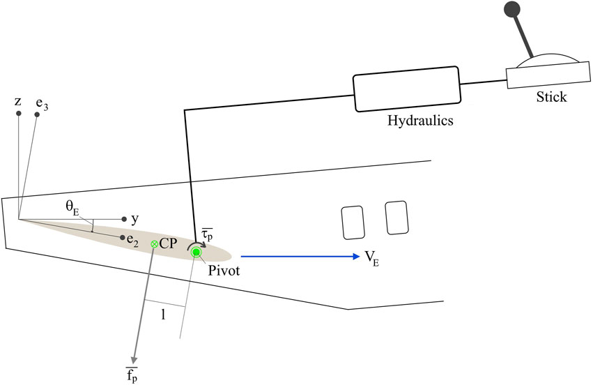
FIGURE 3. Schematic representation of the elevator pivoted to the fuselage. We can see the aft section of the fuselage, minus the vertical tail. In this Figure we assume that the elevator’s velocity V_E is horizontal, for easier understanding. The angle of attack of the elevator is negative, so its lift is negative also.

Let ${\tau }_p{\widehat{\mathbf{e}}}_1$ (where e₁, e₂, e₃ is the elevator airfoil basis) be the torque applied on the elevator by the pilot (the subscript “p” stands for pitch). Since the elevator has an equilibriation timescale much shorter than the whole aircraft, we assume that it is always in a state of torque equilibrium. The only external torque acting on the elevator comes from the lift f_p, as shown in Figure 3. By Eq. 3 and our assumptions of ɛ = 1 and γ = 0, f_p acts through the CP along the e₃-direction; evidently, τ_p = lf_p with l being the distance from the CP to the pivot. Henceforward, we shall treat f_p rather than τ_p as the fundamental pilot-inputted quantity. Let θ_E be the angle which the elevator (i.e., its chord) makes with the y-axis, let V_E be its velocity with respect to the ground and let η′ be the angle between V_E and the y-axis. The angle of attack of the elevator then is α_E = θ_E − η′; expressing (Eq. 3) in terms of magnitude and angle rather than components we have

$f_p=\frac{k_E{V}_E^2}{2}\sin 2{\alpha }_E\text{\hspace{0.17em},\hspace{0.17em}or}(\mathrm{5a})$

${\alpha }_E=\frac{1}{2}\arcsin \frac{2f_p}{k_E{V}_E^2}\Rightarrow {\theta }_E={\eta }^{\prime }+\frac{1}{2}\arcsin \frac{2f_p}{k_E{V}_E^2}.(\mathrm{5b})$

If the stick force is zero, then the elevator floats freely i.e., it lies parallel to the flight path and not to the fuselage. A pull force on the stick, which is required for steady flight, corresponds to negative f_p, so we define the positive ${\bar{f}}_p$ as −f_p. Note that the pivoting location and the “artificial feel” mechanism may change the relationship between the pilot-applied τ_p and f_p; this does not affect the validity of Eq. 5a, b. Also, if the tail has two pieces (separate horizontal stabilizer and elevator), then ${\bar{f}}_p$ will be given by the sum of the forces on both of them.

3.3 Forces and torques

The five forces acting on the aircraft can be seen in Figure 4. They are wing lift (plus induced drag) F, weight $-mg\widehat{\mathbf{z}}$, thrust T, fuselage drag D and tail lift (plus induced drag) ${\bar{\mathbf{f}}}_p$.

FIGURE 4

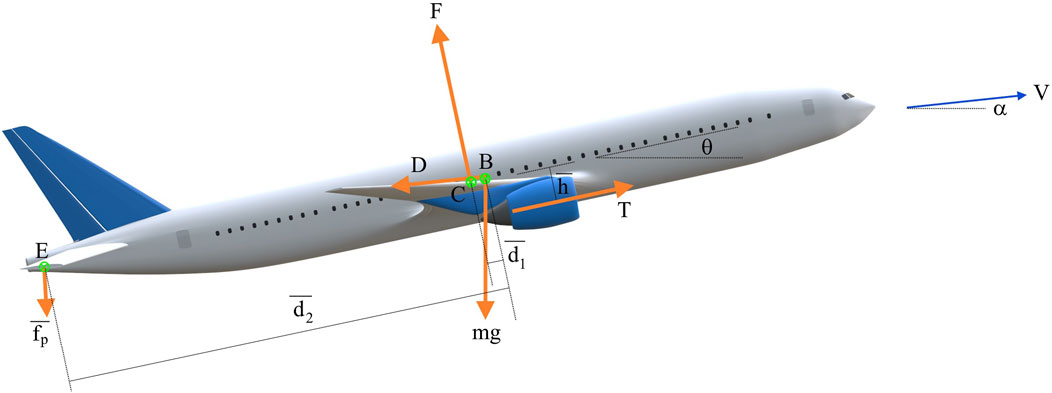
FIGURE 4. Forces acting on the model aircraft. F is the lift, mg the weight, T the thrust and D the drag. Pitch and elevation are 12° and 6°; the elevator deflection is −3° from the flight path and −9° from the fuselage. The directions of all forces as well as the velocity are accurate but their magnitudes are not drawn to scale.

We shall now describe the details of the derivation of the equation of motion. The derivation involves lengthy expressions, so we have used the computer algebra software WXMaxima (Rand and Armbruster, 1987) for it.

We start from the rotation matrices connecting the different bases—y, z attached to the ground, d, o attached to the aircraft and e₂, e₃ attached to the tail. We have

$\left[\begin{array}{c}\hfill {\mathcal{V}}_d\hfill \\ \hfill {\mathcal{V}}_o\hfill \end{array}\right]=\left[\begin{array}{cc}\hfill \cos \theta \hfill & \hfill \sin \theta \hfill \\ \hfill -\sin \theta \hfill & \hfill \cos \theta \hfill \end{array}\right]\left[\begin{array}{c}\hfill {\mathcal{V}}_y\hfill \\ \hfill {\mathcal{V}}_z\hfill \end{array}\right],(\mathrm{6a})$

$\left[\begin{array}{c}\hfill {\mathcal{V}}_2\hfill \\ \hfill {\mathcal{V}}_3\hfill \end{array}\right]=\left[\begin{array}{cc}\hfill \cos {\theta }_E\hfill & \hfill \sin {\theta }_E\hfill \\ \hfill -\sin {\theta }_E\hfill & \hfill \cos {\theta }_E\hfill \end{array}\right]\left[\begin{array}{c}\hfill {\mathcal{V}}_y\hfill \\ \hfill {\mathcal{V}}_z\hfill \end{array}\right],(\mathrm{6b})$

$\left[\begin{array}{c}\hfill {\mathcal{V}}_d\hfill \\ \hfill {\mathcal{V}}_o\hfill \end{array}\right]=\left[\begin{array}{cc}\hfill \cos \left(\theta -{\theta }_E\right)\hfill & \hfill \sin \left(\theta -{\theta }_E\right)\hfill \\ \hfill -\sin \left(\theta -{\theta }_E\right)\hfill & \hfill \cos \left(\theta -{\theta }_E\right)\hfill \end{array}\right]\left[\begin{array}{c}\hfill {\mathcal{V}}_2\hfill \\ \hfill {\mathcal{V}}_3\hfill \end{array}\right],(\mathrm{6c})$

where $\mathcal{V}$ denotes an arbitrary vector. Since rotation matrices are orthogonal, the inverse equals the transpose.

We now write quantitative expressions for each of the forces listed in Figure 4 and the torques which they exert about B.

3.3.1 Wings

Using Eq. 3, the lift is

$\mathbf{F}=-K_C{V}_{Cd}{V}_{Co}\widehat{\mathbf{o}},(7)$

where V_C denotes the velocity of point C. This has two contributions, one from the translation of the aircraft and the other from the rotation of the aircraft about B. That is,

${\mathbf{V}}_C=\mathbf{V}+\omega \widehat{\mathbf{q}}\times d_1\widehat{\mathbf{d}},(8)$

where ω = dθ/dt is the aircraft’s angular velocity. In a typical scenario, the first term outweighs the second by order of magnitude, so we drop the latter and write

$\mathbf{F}=-K_C{V}_d{V}_o\widehat{\mathbf{o}}.(9)$

Note that K_C takes into account both wings. The torque which the lift generates about B is

$\mathbf{\tau }=d_1\widehat{\mathbf{d}}\times F_L\widehat{\mathbf{o}}=d_1{F}_L\widehat{\mathbf{q}}.(10)$

Since d₁ is negative, the torque is negative if the lift is positive, as is evident from Figure 4.

3.3.2 Tail

The force is

$\mathbf{F}=f_p{\widehat{\mathbf{e}}}_3.(11)$

In Eq. 5a, b, V_E has the form ${\mathbf{V}}_E=\mathbf{V}+\omega \widehat{\mathbf{q}}\times d_2\widehat{\mathbf{d}}$; neglecting the second term we can write

${\theta }_E=\eta +\frac{1}{2}\arcsin \frac{2f_p}{k_E{V}^2}.(12)$

Note that η′ of Eq. 5a, b has become η since we have assumed V_E = V. The torque is

$\mathbf{\tau }=d_2\widehat{\mathbf{d}}\times f_p{\widehat{\mathbf{e}}}_3,(13)$

which, using the rotation matrices, gives

$\mathbf{\tau }=f_p{d}_2\cos \left(\theta -{\theta }_E\right)\widehat{\mathbf{q}}.(14)$

When f_p is negative, its torque is positive, consistent with Figure 4.

3.3.3 Thrust

The force is $T\widehat{\mathbf{d}}$ and its torque is $\tau =-Th\widehat{\mathbf{q}}$. Since h is negative, this torque is positive if T is positive, as is clear from Figure 4.

3.3.4 Gravity

The force is $-mg\widehat{\mathbf{z}}$ and the torque is zero since gravity acts through the CM.

3.3.5 Drag

The force is $-C{V}^2\widehat{\mathbf{V}}$ as per Eq. 4. We assume that the fuselage drag acts through the CM, so that its torque can be taken as zero. There is however a drag torque which gets generated when the aircraft rotates in pitch. We model this as a simple damping $\tau =-\mathrm{\Gamma }\omega \widehat{\mathbf{q}}$, where Γ is a constant.

Having obtained all the forces and torques, we substitute them into Newton’s laws of motion.

$m\frac{\mathrm{d}\mathbf{V}}{\mathrm{d}t}=\mathbf{F},(\mathrm{15a})$

$I\frac{\mathrm{d}\omega }{\mathrm{d}t}=\tau .(\mathrm{15b})$

In the second equation above, I is the moment of inertia of the aircraft about the q-axis and the vector nature of ω and τ has been suppressed since they are all about the q-axis.

Using the rotation matrices, we get WXMaxima to express the above five forces in the y-z basis, add them up, and equate the y- and z-components of the resultant force to m times dV_y/dt and dV_z/dt respectively. This generates expressions for dV_y/dt and dV_z/dt. We then implement a variable transformation to express the equations of motion in terms of the speed V and the elevation angle η of the flight path. We have

$V_y=V\cos \eta ,V_z=V\sin \eta ,(16)$

wherefrom

$V={\left(V_x^2+V_y^2\right)}^{1/2}\Rightarrow \frac{\text{d}V}{\text{d}t}=\frac{1}{V}\left(V_y\frac{\text{d}{V}_y}{\text{d}t}+V_z\frac{\text{d}{V}_z}{\text{d}t}\right),(\mathrm{17a})$

$\eta =\arctan \frac{V_z}{V_y}\Rightarrow \frac{\text{d}\eta }{\text{d}t}=\frac{1}{V^2}\left(V_y\frac{\text{d}{V}_z}{\text{d}t}-V_z\frac{\text{d}{V}_y}{\text{d}t}\right).(\mathrm{17b})$

Getting WXMaxima to introduce the expressions for dV_y/dt and dV_z/dt in the above, and also to evaluate the total torque gives us the equation of motion.

We find

$\frac{k_E{V}^2}{2}\sin 2\left(\eta -{\theta }_E\right)={\bar{f}}_p(18)$

and

$\frac{\mathrm{d}y}{\mathrm{d}t}=V\cos \eta (\mathrm{19a})$

$\frac{\mathrm{d}z}{\mathrm{d}t}=V\sin \eta (\mathrm{19b})$

$\frac{\mathrm{d}V}{\mathrm{d}t}=\frac{1}{m}\left[\frac{K_C{V}^2}{4}\left[\cos 3\left(\theta -\eta \right)-\cos \left(\theta -\eta \right)\right]+{\bar{f}}_p\sin \left({\theta }_E-\eta \right)+T\cos \left(\theta -\eta \right)-mg\sin \eta -C{V}^2\right](\mathrm{19c})$

$\frac{\mathrm{d}\eta }{\mathrm{d}t}=\frac{1}{m}\left[\frac{K_{C}V}{4}\left[\sin 3\left(\theta -\eta \right)+\sin \left(\theta -\eta \right)\right]-\frac{{\bar{f}}_p\cos \left({\theta }_E-\eta \right)}{V}+\frac{T\sin \left(\theta -\eta \right)}{V}-\frac{mg\cos \eta }{V}\right](\mathrm{19d})$

$\frac{\mathrm{d}\theta }{\mathrm{d}t}=\omega (19e)$

$\frac{\mathrm{d}\omega }{\mathrm{d}t}=\frac{1}{I}\left[-\mathrm{\Gamma }\omega -\frac{K_C{\bar{d}}_1{V}^2}{2}\sin 2\left(\theta -\eta \right)+{\bar{f}}_p{\bar{d}}_2\cos \left(\theta -{\theta }_E\right)+T\bar{h}\right],(\mathrm{19f})$

which is our proposed closed form model of the aircraft. Equation (19) is a sixth order nonlinear equation set, though the first two equations are decoupled from the rest. It has nine parameters—k_E, m, K_C, C, I, Γ, ${\bar{d}}_1$, ${\bar{d}}_2$, $\bar{h}$ (two more if ɛ and γ are included)—and two external excitation functions T(t) and ${\bar{f}}_p(t)$ which are determined by the pilot or autopilot’s inputs.

4 Results

In this Section, we first present the fixed point and stability analysis of Eq. 19a–f and then demonstrate the manoeuvres. For this, we consider a hypothetical aircraft having the parameter values as given in Table 2. While these values are arbitrary, they have been chosen to create an aircraft with characteristics similar to a 200-seat passenger airliner like the Airbus A321.

TABLE 2

TABLE 2. Parameter values for the model aircraft, which we shall use for the equilibrium and stability analysis as well as for the manoeuvre simulations. m and T denote the maximum possible values of mass and thrust–MTOW or maximum takeoff weight and TOGA or takeoff go around thrust–respectively.

4.1 Equilibria, stability and normal modes

We use the words “equilibrium”, “fixed point” and “steady state” interchangeably, in their dynamical systems sense. For the equilibrium analysis, we treat T and ${\bar{f}}_p$ as constants, which we call T* and f*; let the fixed point values of speed, elevation and pitch be V*, η* and θ*. f* leads to the fixed point tail angle θ_E* via Eq. 18. For the equilibrium analysis, we exclude from consideration Eq. 19a and Eq. 19b since the aircraft cannot be stable to changes in position. In the remaining equations of the set (Eq. 19a–f) we stipulate that the right hand sides be identically zero. This gives us ω* = 0; the remaining variables V*, η* and θ* must satisfy (letting α* = θ* − η*)

$\begin{array}{ll}\hfill & \frac{K_{C}V{*}^2}{4}\left(\cos 3{\alpha }^{*}-\cos \alpha *\right)+f*\sin \left({\theta }_E-\eta *\right)+T*\cos \alpha *\hfill \\ \hfill & -mg\sin \eta *-CV{*}^2=0\hfill \end{array}(\mathrm{20a})$

$\begin{array}{ll}\hfill & \frac{K_{C}V*}{4}\left(\sin 3\alpha *+\sin \alpha *\right)-\frac{f*\cos \left({\theta }_E-\eta *\right)}{V^{*}}+\frac{T*\sin \alpha *}{V^{*}}\hfill \\ \hfill & -\frac{mg\cos \eta *}{V^{*}}=0\hfill \end{array}(\mathrm{20b})$

$-\frac{K_C{\bar{d}}_{1}V{*}^2}{2}\sin 2\alpha *+f*{\bar{d}}_2\cos \left(\theta *-{\theta }_E\right)+T*\bar{h}=0(\mathrm{20c})$

Using the parameter values of Table 2, we solve Eq. 20a–c via Newton-Raphson method and then for stability analysis we substitute the fixed points into the Jacobian of Eq. 19a–f, and calculate its eigenvalues. As a concrete example, we consider stability of fixed points corresponding to level flight (η* = 0) at a range of speeds from 70 to 195 m/s (approximately 250–700 km/h, practical operating speeds near ground). The eigenvalues are shown in Figure 5.

FIGURE 5

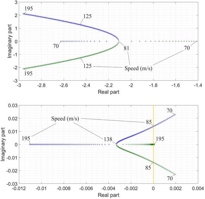
FIGURE 5. Plot of the two pairs of eigenvalues as speed is varied in 200 steps from 70 to 195 m/s. Upper panel shows the short period mode and lower panel shows the phugoid mode. In each panel, blue denotes one eigenvalue and green the other. The speed is labelled on the plot at significant or representative points.

We can see that one mode has real or complex eigenvalues with strongly negative real parts while the other has eigenvalues with real parts whose sign depends on velocity. These are of course the short period and phugoid modes, known to exist for all aircraft. To continue the modal analysis, we now show that the mode shapes corresponding to these eigenvalues are as expected for a typical aircraft. For this, we consider the fixed point corresponding to a speed of 88 m/s at angle of elevation 0. Equation (20a–c) gives the thrust required as 113530 N, the elevator force as 38507 N and the equilibrium pitch as 0.087606 rad. Linearization about this point yields the following eigenvalues and vectors.

${\lambda }_1=-2.1614+\mathsf{j}0.47249,{\lambda }_3=-0.00030416+\mathsf{j}0.012285,(\mathrm{21a})$

${\mathbf{v}}_1=\left[\begin{array}{c}\hfill 0.98363\hfill \\ \hfill -0.087548-\mathsf{j}0.007505\hfill \\ \hfill 0.058969-\mathsf{j}0.026874\hfill \\ \hfill -0.11476+\mathsf{j}0.085947\hfill \end{array}\right],{\mathbf{v}}_3=\left[\begin{array}{c}\hfill 1\hfill \\ \hfill 0.001576-\mathsf{j}0.001285\hfill \\ \hfill -0.000417-\mathsf{j}0.001270\hfill \\ \hfill 0.000016-\mathsf{j}0.000005\hfill \end{array}\right],(\mathrm{21b})$

Where $\mathsf{j}=\sqrt{-1}$. λ₂ and λ₄ are the complex conjugates of λ₁ and λ₃, and the corresponding eigenvectors are conjugates also. We can see that λ₁, v₁ correspond to the short period mode while λ₃, v₃ correspond to the phugoid mode.

To observe the short period behaviour, we set the initial conditions to be V (0) = 88, η(0) = 0–0.01509, θ(0) = 0.087606–0.053748 and ω(0) = 0 + 0.171894. This way of writing highlights the fixed point values plus the perturbations, which are twice the numbers in the imaginary part of v₁ in (21b). We also use y (0) = 0 and z (0) = 300. Figure 6 shows what happens over the next 5 seconds. Within a couple of seconds, the angles attain their equilibrium values. Hence, the short period mode consists primarily of the damping of pitching motions. To observe the phugoid mode, we now use the initial values V (0) = 88, η(0) = 0 + 0.0038547, θ(0) = 0.087606 + 0.0038091 and ω(0) = 0. The perturbations are −3 times the numbers in the imaginary part of v₃ in (21b). We also use y (0) = 0 and z (0) = 300. We plot the results in Figure 7. We can clearly see the long-period oscillation in z and V. The mode eigenvalues and shapes are in accordance with what is known in Literature, thus validating our model (Eq. 19a–f).

FIGURE 6

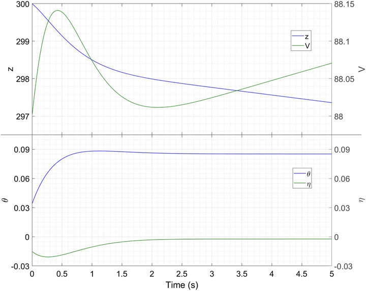
FIGURE 6. Time traces of the variables after an initial perturbation which excites the short period mode. All variables are in SI Units.

FIGURE 7

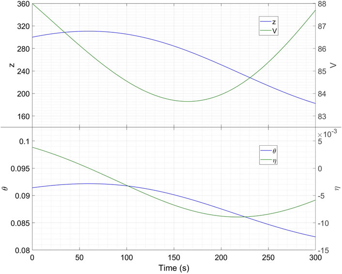
FIGURE 7. Time traces of the variables after an initial perturbation which excites the phugoid mode. All variables are in SI Units.

As another validation procedure, we plot in Figure 8 the thrust T* and pitch θ* corresponding to fixed points at a range of speeds and three different climb rates. From this point onwards, as we gravitate towards more practical applications of aircraft dynamics, we implement a change of Units. It is a fact that aviation features a mix of SI and non-SI Units. Whereas we continue to perform all calculations in SI, we now resort to some non-SI Units in reporting results. This is to achieve partial alignment with the aviation community and increase readability of the manuscript to aircraft operations personnel. For speed, we have used km/h rather than knots (kts) since (a) kts are unfamiliar outside the aviation industry and (b) km/h is the future ICAO recommended unit (ICAO, 2010). For displacements, we use metres for horizontal and feet for vertical. This is because feet for altitudes are ingrained into modern aviation, on account of the minimum safe vertical separation between co-located aircraft being approximately 1,000 ft, and the permissible cruising altitudes thereby being stipulated to be integer thousands of feet. In this case, for Figure 8 we choose speeds ranging from 250–700 km/h and climb rates of 0, 200 and 500 feet per minute (fpm; 1 m/s is very nearly 200 fpm). We call such plots the “characteristics” in line with similar curves for electric motors and generators in electrical engineering (Krishnan, 2010). The V-shaped curve of thrust is familiar.

FIGURE 8

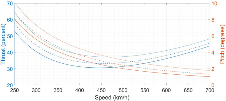
FIGURE 8. Plot of fixed points for the model aircraft. Solid, dashed and dotted lines denote climb rates of 0, 200 and 500 fpm respectively.

Let us consider the fixed thrust level of 40 percent. For each of the three climb rates, this thrust level gives one equilibrium to the right and one to the left of the minima of thrust. We show these equilibria in Table 3.

TABLE 3

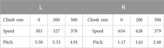
TABLE 3. Climb rate (fpm), speed (km/h) and pitch (degrees) for six equilibria corresponding to 40 percent thrust, with three equilibria to the left of the minima of thrust (L) and three to the right (R).

In the right-hand region, a higher pitch corresponds to a higher climb rate, while in the left hand region, a higher pitch corresponds to a lower climb rate. Moreover, the same power gives a lower speed coupled to a lower climb rate on the left. These are well-known performance features of aircraft (Langewiesche, 1944; Hurt, 1959; Barnard and Philpott, 2010; Cae Oxford Aviation Academy, 2014; Badick and Johnson, 2022) the two regions are called the regions of normal command (right) and reversed command (left).

Thus, our new model (Eq. 19a–f) has successfully yielded the textbook results thereby demonstrating that it is as capable as the traditional models of predicting the equilibria and stability of the aircraft.

4.2 Manoeuvre analysis

Having validated the model, we now turn to its central use, which is the explicit demonstration of manoeuvres. We will first plan the manoeuvres qualitatively and quantitatively basis the model and then use the equations of motion in a simulator environment to show the details of the execution. We consider two speciality manoeuvres, the Immelmann turn and the vertical dive. In this article, we focus on these two manoeuvres rather than the mainstays of civilian aviation (takeoff, landing, etc.) to keep the treatment brief. Any analysis of civilian aviation, if we are to perform it with the thoroughness it deserves, will require an extended discussion of safety as well as performance, and we leave this heavy lifting to future work. Despite our chosen manoeuvres being more suited to tailormade aircraft, here we exploit the advantages of the virtual environment to retain the model aircraft of Table 2. We do however reduce its mass to m = 80000 kg to generate a greater thrust-to-weight (and drag-to-weight) ratio.

In Figure 9 we plot the characteristics for this aircraft. Structurally similar to Figure 8, the three climb rates this time are 0, 1,000 and 3,000 fpm respectively (typical climb rates in a civilian context). We also show the required ${\bar{f}}_p$ in a separate panel. These plots will help us execute the manoeuvres.

FIGURE 9

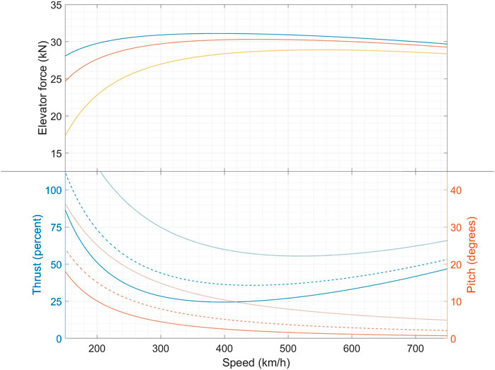
FIGURE 9. Characteristics for the model aircraft with m = 80 tons.

To execute and demonstrate the manoeuvres, we use Eqs 18, 19a–f to set up a flight simulator with a basic user interface. We call this the academic flight simulator, and intend it to be the primary realization of our model in the flying school environment. The simulation proceeds in discrete cycles of user-defined time duration (here we have chosen 1 s of flight time per cycle). At the completion of each cycle, the machine displays to the user the values of relevant variables such as speed, altitude and pitch (the specific instruments simulated vary by manoeuvre—during a simulation of landing for instance, we show the deviation from the glideslope), and invites the user to enter the values of T and ${\bar{f}}_p$ to be used during the next cycle. The user makes these inputs basis of the displayed variables, just as in a real flight the pilot adjusts his/her control inputs in reaction to the instrument readings. Unlike in a real-time flight simulator, the pauses at the end of each cycle in the academic flight simulator allow the user to think carefully and come up with an optimal input. In our opinion, this maximizes the learning outcomes. Once the inputs are received, the simulator then substitutes these values into Eqs 18, 19a–f, and numerically integrates them over the duration of the cycle using the initial conditions from the end of the preceding cycle (for the first cycle, the initial conditions are defined by the user). Integration method is fourth order Runge Kutta with a time step of 10^–4 s.

Given the academic flight simulator, we have used it to obtain the input signals for the manoeuvres through the time-honoured strategy of practice makes perfect. Operating the simulator ourselves just as a student pilot would, we have continually refined our inputs to make the manoeuvre approach closer and closer to the stated targets. Once our execution has attained demonstration quality, we have then included the attempt in this article. Thus, we can say that our input histories for each manoeuvre are based on human learning from the model-generated data.

4.2.1 Immelmann turn

This manoeuvre consists of a 180° vertical loop from straight flight to inverted flight on the reciprocal heading, followed by a 180° bank to cancel the inversion. Here we shall analyse only the half-loop as that takes place in the pitch plane alone. To pull an Immelmann turn, we need to command high ${\bar{f}}_p$ (for the simulation we choose 100 kN) so as to pitch up rapidly. At the end of the manoeuvre, when the aircraft is inverted, the lift required to balance gravity must be negative (relative to the aircraft’s d, o axes), so α and ${\bar{f}}_p$ must be negative also. Since α is always small, positive ${\bar{f}}_p$ gives positive torque and the transition from high positive to negative ${\bar{f}}_p$ at the end of the manoeuvre should automatically cause the desired sign change of α as well. A climb against gravity will require as much thrust as possible to minimize the loss of speed, so the thrust remains set to 99 percent throughout. Figure 10 shows a schematic representation of the trajectory together with the aircraft itself at suitable intervals on it. Figure 11 shows the time traces of the pilot’s commands and the most significant dynamical variables.

FIGURE 10

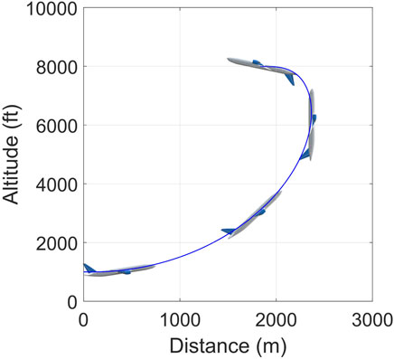
FIGURE 10. Profile of the model aircraft during the Immelmann manoeuvre. The trajectory is to scale and the pitch is accurate but the aircraft itself is over-large for clarity. The high negative α in the last snapshot is noteworthy.

FIGURE 11

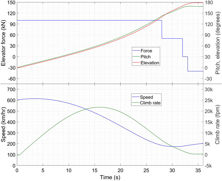
FIGURE 11. Time traces of different variables during the Immelmann manoeuvre. The elevation is the flight path angle η. The symbol “k” denotes thousand.

High ${\bar{f}}_p$ causes both pitch and elevation to increase quickly. The first reduction of ${\bar{f}}_p$ causes α to flip sign while further reduction to negative values stabilizes η at 180°, just as we expected. The speed drops sharply as the aircraft climbs through a significant altitude, explaining the asymmetry between distance and pitch in Figure 10.

4.2.2 Vertical dive

The dive has three parts—preparation for the dive, entry into the dive and exit from the dive. In the preparation phase, we decelerate to level flight at the slowest possible speed. To achieve this, we retard throttles to idle (here assumed 10 percent of TOGA thrust); since angle of attack must increase as speed decreases, a gradual raising of the nose is required during deceleration. When α approaches the stalling value (here taken to be 15°), we initiate the dive by pushing the nose down. The target for the dive has to be η = θ = −90°; (Eq. 19a–f); admits such a solution with ${\bar{f}}_p=0$ and V increasing monotonically upto the terminal velocity (whatever it may be). The strongly stable short period mode at all relevant speeds suggests that this state, once entered, will be stable to deviations in θ. To reach η = −90°, we need to eliminate the y-component of velocity present at the initiation of the dive. When the aircraft’s nose is below horizontal, a negative α will result in the lift’s acquiring the desired −y-component; this α must however be sufficiently small in size as to prevent the aircraft from entering retrograde motion (η < − 90°). Since negative lift causes a nose-up moment, a fairly strong nose-down elevator must be applied to counteract it and hold α steadily negative. As η approaches −90°, we will need to reduce the elevator force to bring α closer to zero, ideally reaching this state at the same instant as η reaches −90°. After the dive is over, exit will have to be achieved using maximum nose-up elevator input, and when a climb is established, we will need to reapply thrust. Let us specify a target climb rate of 3,000 fpm for this phase of flight.

Figures 12, 13 show the aircraft profile and the relevant time traces. The ideal dive (η = θ = −90°) is held from t = 32 to t = 35 s. We can see that the elevator states attained through practice on the simulator are close to the predictions of Figure 9 wherever the latter are applicable. For instance, during the preparation phase, Figure 9 suggests ${\bar{f}}_p$ just above 30 kN to maintain equilibrium flight at 250 km/h and below; Figure 13 shows a slightly higher elevator force being required since we need to raise the nose as well. Again during the pull-up phase, when the climb rate reaches close to 3,000 fpm, the speed is about 580 km/h. Figure 9 suggests for this operating condition a thrust of about 55 percent and ${\bar{f}}_p$ of about 29 kN. In the last 11 s of Figure 13 we can see that 60 percent thrust and alternating elevator force between 28 kN and 30 kN give us a steady 3,000 fpm climb with a very slow acceleration.

FIGURE 12

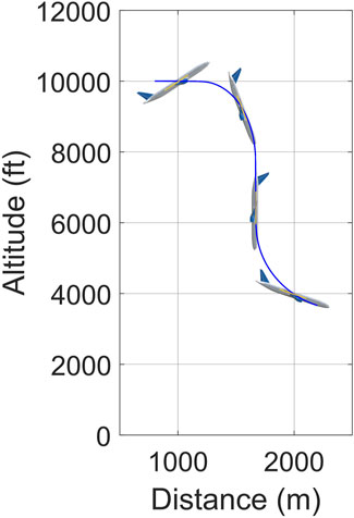
FIGURE 12. Schematic profile of the model aircraft during the most important portion of the vertical dive (from approximately t =12 to t =41 s of the simulation). The trajectory is to scale; for clarity, the aircraft is over-large, the d-axis is highlighted by a yellow line and the angle of attack is enlarged by a factor of three, thus θ in the Figure is η +3α. We can see α varying from snapshot to snapshot–it is very high positive in the first to balance the weight at a low speed, low negative in the second to retard the forward speed, zero in the third by design and moderately high positive in the fourth which combines with the high speed to generate a lift significantly exceeding the weight.

FIGURE 13

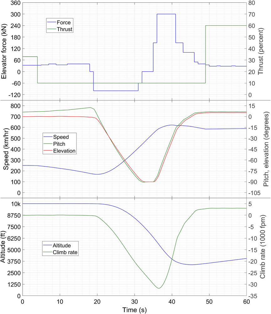
FIGURE 13. Time traces of different variables during the vertical dive. The elevation is the flight path angle η. The symbol “k” denotes thousand.

5 Discussion

In our planning of the dive, we saw one concrete instance where dynamical systems theory as applied to the closed-form model (Eq. 19a–f) gave us the existence as well as the stability of the solution $\theta =\eta ={\bar{f}}_p=0$. It would have been far more difficult to extract this solution from a data table model. Similar advantages, on a much larger scale, pertain to calculations of takeoff, landing and civilian aviation manoeuvres, as will be shown in future works. It is also interesting that a model-based treatment is sometimes capable of greater accuracy than a qualitative treatment alone. In Langewiesche’s pioneering work (Langewiesche, 1944), we find in Chapter 2 a discussion of “the airplane’s gaits”. Two of these gaits are level flight at low and high α′s while two more relate to steady climbs and descents. In our view, all these (and everything in between) are pitch plane equilibria, as shown in Figures 8, 9. Corresponding to each steady state flight condition we have a required thrust, pitch attitude and elevator trim. A further gait in Langewiesche (1944) is the dive; the book says that for a vertical dive, one must have the nose pointing slightly backward, i.e., if η = −90° then θ < − 90°. From our analysis, we can see that a negative α is required during dive entry but α = 0 suffices during the vertical portion of the dive.

An additional advantage of our model-based manoeuvre analysis is the introduction of the aircraft characteristics, as in Figures 8, 9. With the exception of the power curve—a plot of thrust vs. speed for level flight which makes no reference to the elevator state—such characteristics do not appear in existing Literature. They do however have significant utility in manoeuvre planning and execution. In this article they yielded the values of T and ${\bar{f}}_p$ to be used for the 3,000 fpm climb at the end of the dive in Figure 13. Characteristics were not used more extensively here because the rest of the manoeuvres did not feature equilibrium flights; civil aviation manoeuvres do so to a much greater extent.

With respect to the limitations of the study, we have already mentioned that the empirical lift formula Eq. 3 is not equipped to describe the flow field around the aircraft and hence is not applicable to studies involving multiple mutually interacting aircraft (formation flight, wake turbulence). We have also enunciated that this limitation does not carry over to the analysis of a single aircraft, which is the topic of this article (and indeed, of almost the entire flight dynamics Literature). In Table 4, we enumerate the assumptions in the model and the expected consequences of relaxing these assumptions.

TABLE 4

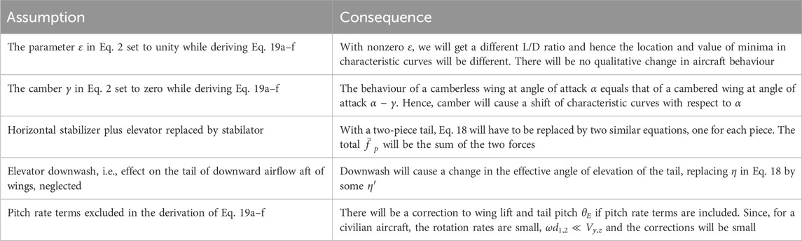
TABLE 4. Table showing the assumptions in the model and the anticipated results of relaxing these assumptions.

Further, in the simulations here, we have used a model of a passenger airliner to demonstrate speciality manoeuvres. This is because of our plan to use the same model aircraft to demonstrate manoeuvres pertinent to civil aviation. Many acrobatic stunts are prohibited for passenger airplanes not for reasons of dynamical feasibility but because the resulting stresses may exceed the airframe’s ultimate design limit. On a simulator of the dynamics alone, this is not a relevant factor. In these simulations, we have also implemented altitude changes of several thousand feet without varying K_C, k_E and C to account for the dependence on air density. This is for simplicity and in our opinion is acceptable as long as we are aware of it; incorporating the density will not introduce any qualitatively significant changes to the dynamics, and the model aircraft is a hypothetical one anyway.

6 Conclusion and future directions

In this article we have proposed a closed form dynamic model for the pitch plane or longitudinal motions of an aircraft. After validating it by the derivation of standard results, we have shown how it can be used to plan and execute two acrobatic manoeuvres. Demonstration of many more manoeuvres such as takeoff, landing and stall recovery are planned for the immediate future. Our hybrid of theory and practice makes our work equally applicable to the university and the flying school.

Here, our demonstration aircraft has been a fictitious model. Future work will aim to create models of real airliners such as Airbus A320 and Boeing 777. Since the (pitch plane) model has only eleven unknown parameters and no unknown functions, it should be possible to estimate the best-fit values of these parameters from flight data recorder observations alone. To the best of our knowledge, no public domain model exists for a passenger airplane. A more distant future work is the extension of the model (Eq. 19a–f) to the general case of three dimensions, which will enable us to plan and demonstrate all possible manoeuvres.

Currently, we are seeing a global surge in demand for pilots on account of rapid growth in the airline industry. Due to the rigorous training requirements for air transport pilots, such demand is not easy to satisfy quickly. If the on-ground pilot training program is modified to include model-based manoeuvre analysis, then it may be possible to expedite the ground training phase without compromising pilot proficiency and safety. Model-based pilot training might also help to improve safety standards in general and non-transport commercial aviation, where accidents due to pilot error are far more prevalent than in airline flights. Of course, all these are still very much future possibilities. But as they say, the journey of eight thousand miles begins with a mile-and-a-quarter takeoff, and our article shows a credible path towards such a future. Demand for UAV pilots is also expected to rise significantly over the coming years due to proliferation of drones for transport and delivery purposes. We are currently far from a systematization and formalization of a drone training curriculum, and building in a model-based component at the outset might well be beneficial for the safety and efficiency of UAV operations. Concurrently, introduction of some applied aspects into the university flight dynamics curriculum will enable the aerospace engineering graduates to get a greater feel for the practical consequences of the mathematical equations, and will be especially useful in preparing them for a career in industry.

In conclusion, our article shows the beginnings of a new approach to flight dynamics which synthesizes the Bryan and Langewiesche philosophies; in future we hope to see a further unification of these two branches, and reap the theoretical as well as practical benefits of such a synergy.

Data availability statement

The original contributions presented in the study are included in the article/Supplementary material, further inquiries can be directed to the corresponding authors.

Author contributions

BS: Conceptualization, Formal Analysis, Investigation, Software, Supervision, Writing–original draft, Writing–review and editing. SG: Software, Visualization, Writing–review and editing. SM: Software, Visualization, Writing–review and editing.

Funding

The author(s) declare that no financial support was received for the research, authorship, and/or publication of this article.

Acknowledgments

We would like to thank the Reviewers for their suggestions which have resulted in substantial improvement to the quality of this manuscript. SG gratefully acknowledges support of the Department of Atomic Energy, Government of India, under project no. RTI4001.

Conflict of interest

The authors declare that the research was conducted in the absence of any commercial or financial relationships that could be construed as a potential conflict of interest.

Publisher’s note

All claims expressed in this article are solely those of the authors and do not necessarily represent those of their affiliated organizations, or those of the publisher, the editors and the reviewers. Any product that may be evaluated in this article, or claim that may be made by its manufacturer, is not guaranteed or endorsed by the publisher.

References

Anderson, J. D. (1989). Introduction to flight. Third Edition. New York City, USA: McGraw Hill.

Google Scholar

Badick, J. R., and Johnson, B. A. (2022). Flight theory and aerodynamics. Fourth Edition. New York City, USA: Wiley.

Google Scholar

Barnard, R. H., and Philpott, D. R. (2010). Aircraft flight. Fourth Edition. Upper Saddle River, USA: Pearson.

Google Scholar

Etkin, B. (1971). Dynamics of atmospheric flight. Second Edition. New York City, USA: Dover Publications.

Google Scholar

Bryan, G. H. (1911). Stability in aviation. London, UK: Macmillan.

Google Scholar

CAE Oxford Aviation Academy (2014). Principles of flight. Singapore: KHL Printing Company.

Google Scholar

Caughey, D. A. (2011). Introduction to aircraft stability and control. Ithaca, NY: ebook. Available at: https://courses.cit.cornell.edu/mae5070/Caughey_2011_04.pdf.

Google Scholar

Gonzalez, C., and Taha, H. E. (2022). A Variational theory of lift. J. Fluid Mech. 941, A58. doi:10.1017/jfm.2022.348

CrossRef Full Text | Google Scholar

Guicheteau, P. (1998). Bifurcation theory: a tool for nonlinear flight dynamics. Philosophical Trans. R. Soc. A 356 (1745), 2181–2201. doi:10.1098/rsta.1998.0269

CrossRef Full Text | Google Scholar

Hassan, A. M., and Taha, H. E. (2017). Geometric control formulation and nonlinear controllability of airplane flight dynamics. Nonlinear Dyn. 88 (4), 2651–2669. doi:10.1007/s11071-017-3401-9

CrossRef Full Text | Google Scholar

Hess, R. A., Gao, C., and Wang, S. H. (1991). Generalized technique for inverse simulation applied to aircraft maneuvers. AIAA J. Guid. 14 (5), 920–926. doi:10.2514/3.20732

CrossRef Full Text | Google Scholar

How, J. (2004). Aircraft stability and control. MIT OpenCourseWare. Available at: https://ocw.mit.edu/courses/16-333-aircraft-stability-and-control-fall-2004/.

Google Scholar

Hurt, H. (1959). Aerodynamics for naval aviators. Washington DC, USA: US Naval Air Systems Command.

Google Scholar

ICAO (2010). “Units of measurement to be used in air and ground operations,” in Annexe 5 to the Convention on International Civil Aviation.

Google Scholar

Jahnke, C. C. (1990). Application of dynamical systems theory to nonlinear aircraft dynamics. Pasadena, USA: Doctoral thesis, California Institute of Technology.

Google Scholar

Krishchenko, A. P., Kanatkikov, A. N., and Tkachev, S. B. (2009). “Planning and control of spatial motion of flying vehicles,” in Proc. IFAC Workshop Aerosp. Guid. Navigation Flight Control Syst.

Google Scholar

Krishnan, R. (2010). Electric motor drives: modelling, analysis and control. New Delhi, India: PHI Learning Private Limited.

Google Scholar

Lanchester, F. W. (1908). Archibald Constable of London. London, UK.

Google Scholar

Langewiesche, W. (1944). Stick and rudder. New York City, USA: McGraw Hill.

Google Scholar

Liu, T. (2023). Can lift be generated in a steady inviscid flow. Adv. Aerodynamics 5, 6. doi:10.1186/s42774-023-00143-3

CrossRef Full Text | Google Scholar

Lone, M., and Cooke, A. (2014). Review of pilot models used in aircraft flight dynamics. Aerosp. Sci. Technol. 34, 55–74. doi:10.1016/j.ast.2014.02.003

CrossRef Full Text | Google Scholar

Lowenberg, M. H., and Champneys, A. R. (1998). Shil'nikov homoclinic dynamics and the escape from roll autorotation in an F–4 model. Philosophical Trans. R. Soc. A 356 (1745), 2241–2256. doi:10.1098/rsta.1998.0272

CrossRef Full Text | Google Scholar

Macmillen, F. B. J. (1998). Nonlinear flight dynamics analysis. Philosophical Trans. R. Soc. A 356 (1745), 2167–2180. doi:10.1098/rsta.1998.0268

CrossRef Full Text | Google Scholar

Murray-Smith, D. J., and Mcgookin, E. W. (2015). A Case study involving continuous system methods of inverse simulation for an unmanned aerial vehicle application. Proc. Institution Mech. Eng. Part G J. Aerosp. Eng. 229 (14), 2700–2717. doi:10.1177/0954410015586842

CrossRef Full Text | Google Scholar

Nelson, R. C. (1998). Flight stability and automatic control. Second Edition. New York City, USA: McGraw Hill.

Google Scholar

Noronha, N. P., and Krishna, M. (2021). Aerodynamic performance comparison of airfoils suggested for small horizontal-axis wind turbines. Mater. Today Proc. 46 (7), 2450–2455. doi:10.1016/j.matpr.2021.01.359

CrossRef Full Text | Google Scholar

Padfield, G. D. (2011). The Tau of flight control. Aeronautical J. 115 (1171), 521–556. doi:10.1017/s0001924000006187

CrossRef Full Text | Google Scholar

Pamadi, B. (1998). Performance, stability, dynamics and control of airplanes. Reston, USA: AIAA.

Google Scholar

Phillips, W. (2004). Mechanics of flight. Hoboken, USA: Wiley.

Google Scholar

Rand, R. H., and Armbruster, D. (1987). Perturbation methods, bifurcation theory and computer algebra. Heidelberg, Germany: Springer Verlag.

Google Scholar

Regis, E. (2020). “No one can explain why planes stay in the air”. Scientific American. Available at: https://www.scientificamerican.com/article/no-one-can-explain-why-planes-stay-in-the-air/.

Google Scholar

Rohith, G., and Sinha, N. K. (2020). Routes to chaos in the post-stall dynamics of higher-dimensional aircraft model. Nonlinear Dyn. 100 (2), 1705–1724. doi:10.1007/s11071-020-05604-8

CrossRef Full Text | Google Scholar

Saarlas, M. (2007). Aircraft performance. New York City, USA: Wiley.

Google Scholar

Saetti, U., and Horn, J. H. (2022). Flight simulation and control using the JULIA language. AIAA Scitech Forum. doi:10.2514/6.2022-2354

CrossRef Full Text | Google Scholar

Sinha, N. K., and Ananthkrishnan, N. (2014). Elementary flight dynamics with an introduction to bifuraction and continuation methods. Boca Raton, USA: CRC Press.

Google Scholar

Sinha, N. K., and Ananthkrishnan, N. (2017). Advanced flight dynamics with elements of flight control. Boca Raton, USA: CRC Press.

Google Scholar

Stengel, R. F. (2004). Flight dynamics. Princeton, USA: Princeton University Press.

Google Scholar

Thomson, D., and Bradley, R. (2006). Inverse simulation as a tool for flight dynamics research: principles and applications. Prog. Aerosp. Sci. 42 (3), 174–210. doi:10.1016/j.paerosci.2006.07.002

CrossRef Full Text | Google Scholar

Webb, J., Higgenbotham, H., Liebshutz, D., Potts, D., Tondreau, E., and Ashworth, J. (2001). “Analysis of Gurney flap effects on a NACA0012 airfoil/wing section,” in AIAA 19th Applied Aerodynamics Conference (Anaheim, CA).

CrossRef Full Text | Google Scholar

Zhukovsky, N. E. (1949). On Bird hovering. Collect. Works Vol. 4.

Google Scholar