A hybrid long short-term memory with generalized additive model and post-hoc explainable artificial intelligence with causal inference for air pollutants prediction in Kimberley, South Africa

The study addresses the problem of nonlinear characteristics of common air pollutants by proposing a deep learning time-series model based on the long short-term memory (LSTM) integrated with a generalized additive model (GAM). LSTM model captures both nonlinear relationships and temporal long-term dependencies in time-series data, and GAM provides insight into the statistical relationship between selected features and the target pollutant. The post-hoc eXplainable artificial intelligence (xAI) technique, local interpretable model-agnostic explanation (LIME), further explains the nonlinearity. Finally, causal inference was determined on the impact of the air pollutants relationship, thereby offering further interpretability in which deep learning models are deficient. Meteorological and air pollutant statistical records were leveraged from a Hantam (Karoo) air monitoring station in South Africa, and through a random sampling approach, synthetic data were generated for the city of Kimberley. The model was evaluated with the mean squared error (MSE), root mean squared error (RMSE) and mean absolute error (MAE) for different time-steps. The proposed referred to as long short-term memory generalized additive model based post-hoc eXplainable Artificial Intelligence (LSTM-GAM_xAI) model with a 10-day time-step and 5-day time-step for multiple pollutants prediction guaranteed least MSE. Though the causal effect analysis show no p-values (>0.88) for variables, the experiment results show that LSTM-GAM-xAI guaranteed the lowest MSE values across different time-steps.

1 Introduction

The prediction of air pollutant concentration continues to receive attention from the research community due to the health risk impact of high levels of air pollutant concentrations. Despite the World Health Organization (WHO) standard limits on the allowable air pollutant concentration in the environment, the problem of air pollution persists in some countries. Some of the sources of these air pollutants include power plants and cement factories, and the transport sector, which are known to emit Nitrogen Dioxide (NO₂) into the atmosphere (Tu et al., 2023).

Air is a combination of gaseous components, and understanding the correlation is key, which can equally be achieved with machine learning or deep learning time-series models. Deep learning models for time-series analysis find patterns in the air pollutant dataset to help understand the nature of correlation through their network architecture. For instance, deep learning models such as the long short-term memory model (LSTM) use their gated mechanism to filter the necessary data inputs to produce refined output. Generally, LSTM is one of the commonly used models for time-series analysis, which requires training and testing with volumes of data. Other variants of deep learning models includes bi-directional LSTM (BiLSTM), gated recurrent unit (GRU), bi-gated recurrent unit (BiGRU), and one-dimensional convolutional neural network (1DCNN). These model, among other time-series models, captures complex nonlinear and temporal long-term dependencies in air pollutants (Agbehadji and Obagbuwa, 2025a). Mostly, air pollutants exhibit dynamic tendencies that make their modeling challenging. In this regard, the modeling of air quality tasks is not immune to errors that could impact on model’s performance. Several attempts have been made by researchers to address the errors from either a data or a model structure perspective. For instance, the use of an adaptive Kalman filter in an LSTM model to address prediction performance and also noise in the dataset (Agbehadji and Obagbuwa, 2025b). Again, the ensemble Kalman Filter was integrated with machine learning and deep learning models for long-term forecasting to reduce the level of uncertainty in data-driven models (Cheng et al., 2023). Therefore, hybrid models have contributed greatly to enhancing predictive accuracy in most prediction tasks. Wahiduzzaman and Yeasmin (2024) enhanced the predictive capability of deep learning models by utilizing a generalized additive model (GAM) to smooth the transformation of predictors. GAM is a machine learning model that helps to capture nonlinearity in data through its smoothing function capability (Tyralis and Papacharalampous, 2024). One of the potential of GAM is that it help understand problems within relevant domains such as air pollution to help stakeholders formulate their policies. Again, it help to bridge the gap between traditional statistical models and machine learning or deep learning models which make it a very valuable tool in xAI. While the role of neural-based GAM has been identified to provide interpretable and transparent deep learning models (Ortega-Fernandez et al., 2024), understanding the causal effect of air pollutants in a predictive task remains a challenge.

To solve the aforementioned challenge, this study attempts to develop a novel air predictive model for Kimberley. Kimberley is located in the Northern Cape Province of South Africa. The Northern Cape covers an area of 372,889km² with an estimated population of 1,193,780. The Province is rich in minerals and also has fertile agricultural land (Department of Environmental Affairs, 2019). Figure 1 shows the map of South Africa with air monitoring stations.

Figure 1

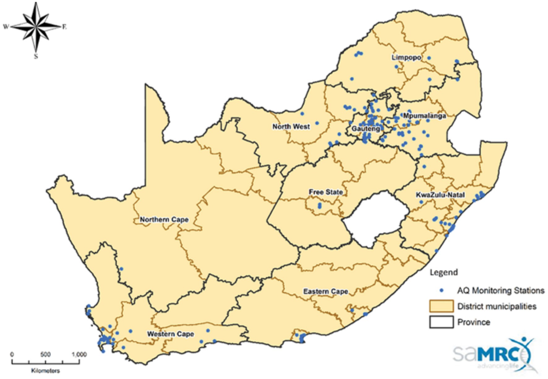
Figure 1. Map of South Africa showing Air quality monitoring stations in South Africa as of January 2023.

In Kimberley, the leading air pollution sources are diamond mining activities, vehicle emissions, and industrial facilities, where particulate matter (PM_2.5) is a primary concern (Becker et al., 2024). Moreover, the annual measure of particulates (PM₁₀) and sulfur dioxide (SO₂) are the two most prevalent pollutants in South Africa (Forestry Fisheries and the Environment, 2024). Furthermore, power stations in South Africa emit different kinds of air pollutants, including Carbon Monoxide (CO), NO₂, and sulfur dioxide (SO₂) (Agbehadji and Obagbuwa, 2025a). Unfortunately, the activities of large-scale diamond mining companies in Kimberley impact negatively on the environment, leading to land degradation, air pollution and biodiversity loss (Charumbira and Ncube, 2022).

This study aims to develop a model for predicting multiple air pollutant concentrations including PM_2.5, PM₁₀, Ozone (O₃), SO₂, NO₂, NO, and NO_x. Additionally, meteorological factors such as wind speed (WS), ambient temperature (AT), relative humidity (RH) and solar radiation (SR) were considered in developing the predictive model. The generalized additive model (GAM) and deep learning time-series models, such as LSTM, were utilized for nonlinear relationship modeling and capturing temporal dependencies in the pollutants dataset. A causal inference model is leveraged to establish the impact of predicted air pollutants and others. Given that deep learning models have complex network structures, hybridizing with another model could increase the level of complexity, thus, the post-hoc explanation is employed to explain the feature influences on target variables and the model complexity. The post-hoc techniques, such as LIME, are gaining popularity in providing explanations on the relationship between a target and predictors, and provide feature importance to help with human understanding. Our study contributes toward developing a predictive model for air monitoring stations that seek to use an enhanced deep learning model with causal inference capability, as an alternative to legacy-based air pollutant concentration prediction systems. The sections are section 2 (literature review), section 3 (Method and material), section 4 (results), section 5 (discussion), section 6 (methodological limitations) and section 7 (conclusion).

2 Literature review

This section presents a review of generalized additive models, deep learning time-series models and post-hoc explanation models focusing on air pollutant concentration prediction within their air quality thresholds. It then presents a summary of models, either single or hybrid models, applicable to diverse research domains within the context of air pollution predictions and quality indexes.

2.1 Generalized additive model

The GAM is a model that handles the nonlinear relationship among features. GAM handle this nonlinearity through the use of link functions to map input data to their search space (Nisbet et al., 2009). By so doing, it uses probability distributions to achieve the mapping to the data distribution. This model incorporates smoothing functions (like splines) to model the relationship, thereby allowing the capture of the nonlinearity in data variables. By so doing, it offers interpretability to models. Additionally, neural networks, when deployed on GAM, can estimate the smoothing function to offer scalable models. The degree of flexibility of the GAM makes it suitable for its incorporation in other models. Jo and Kim (2023) indicated that using neural networks on GAM offers good prediction performance for multivariate time-series predictions (MTS) and also offers interpretability for neural networks (which are black-box in nature). Integrating a neural network on GAM helps estimate each feature contribution toward an accurate and explainable deep learning model (Ortega-Fernandez et al., 2024). Studies such as Lou et al. (2012) and Obster et al. (2022) also applied machine learning models to GAM to enhance accuracy. Studies have been conducted to compare the utilization of interpretability of tools like GAM and Shapley additive explanations (SHAP) among scientists and concluded that there is over-trust and misuse of these tools (Kaur et al., 2020). Given this, the merit and demerits of GAM and machine learning models were highlighted, thus discounting the notion that there is no strict trade-off between models’ performance and interpretability, thereby dispelling the idea that only black box models can achieve high performance (Kruschel et al., 2025).

Since deep learning time series models can handle nonlinear relationships as well as GAM can also handle nonlinear relationships, presenting a common approach for integration. Thus, the two-layer approach can help to improve the accuracy of models. Within a search space, the GAM can search for nonlinear transformations of both target and predictors that can result in additive model. Though GAM is a statistical tool, it provides more analytical tools for climate modeling than traditional linear models (Ravindra et al., 2019). The GAM is also very effective at handling time-series data. GAM provides a best fit for non-linear relationships between the independent variable and the predictor (Ravindra et al., 2019). However, the ease of understanding the output of the model has been a challenge when more complex nonlinear models are utilized in the prediction.

Bai et al. (2021) indicated that air quality standards are not static and need to be revised after a certain period. For instance, in 2013, China developed new air quality standards in which the GAM was used to evaluate this new standard on air pollutants such as PM₁₀, SO₂, and NO₂. Their findings suggest that the new standard affected the health of the population (Bai et al., 2021). Barbalat et al. (2024) used the GAM to aggregate the prediction of three machine learning models, such as extreme gradient boosting, random forest and categorical boosting, to predict daily NO₂ concentration with low error levels. In this regard, combining the predictions increases the chance of an accurate prediction over time. The GAM has been extensively applied to analyze the relationship between air pollutants, environmental factors and health-related issues (Gao et al., 2025; Fu et al., 2023; Fu et al., 2020; Fang et al., 2021; Fan et al., 2024; Gu et al., 2020). Common air particles such as PM₁₀ can remain in the atmosphere for minutes or hours, whereas PM_2.5 can remain for days or weeks.

GAM demonstrates optimal performance in capturing the nonlinear relationship between concentration O₃ and predictor factors than the multiple linear regression model for different locations (Habeebullah, 2020). GAM is also able to disclose the varying dependencies between air pollutants (such as PM₁₀ and NO₂) and meteorological variables for different locations and seasons (Haddad and Vizakos, 2021). Table 1 presents research on the use of GAM in different research domains.

Table 1

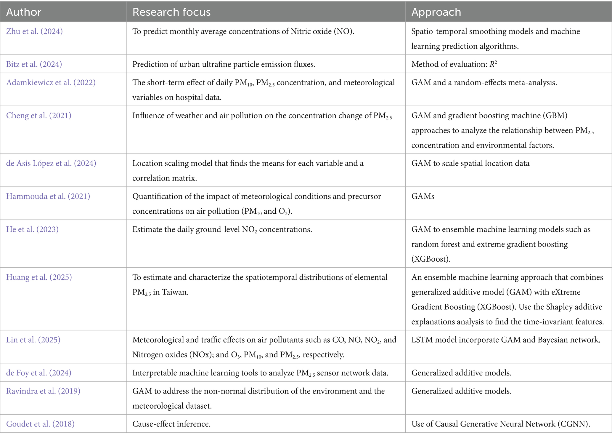
Table 1. Generalized additive model in air pollution.

Despite the application of generalized additive models (GAMs), it lacks structures that offer the needed scalability when large volumes of data are required (Chang et al., 2022). GAM is more interpretable than models such as post-hoc explanations (SHAP) (Kaur et al., 2020). The hybridization of GAM with deep learning models such as GRU, BiLSTM, and 1DCNN remains a research domain that needs to be explored within the context of air pollution prediction. Therefore, applying GAM, this research provides two insights: that is model’s interpretability and performance.

2.2 Time-series deep learning models

Many attempts have been made to improve the interpretability of deep learning models, leading to the use of models such as neural-based GAM and post-hoc models (such as SHAP). The gradient-based approach (such as the Adam method) has been used as an approach to smooth parameters used in GAM (Dammann et al., 2025). Deep learning models have multiple layers to process input data, reveal the hidden structures in a large set of data, improve training and model’s performance (LeCun et al., 2015). Deep learning also has “Dropout” as a way to prevent overfitting in deep learning models (Srivastava et al., 2014).

Setianingrum et al. (2022) suggested the use of the Prophet Facebook model and the Bayesian Optimisation as a hyper-parameter tuner to effectively predict O₃, SO₂, and CO. While traditional models like autoregressive integrated moving average (ARIMA) are more accurate for predicting the parameters of PM₁₀ and NO₂. Since model performance differs across different air pollutant datasets, there is a need to continuously enhance the model’s performance. Eslami et al. (2020) indicated that the convolutional neural network (CNN) model is faster in predicting hourly O₃ concentrations throughout the year than both LSTM and deep stacked auto-encoder (SAE). Also, the CNN predictions of daytime O₃ concentrations were more accurate than nighttime. However, the CNN model under-predicted the daily maximum ozone concentrations, particularly during the summer, because of the non-availability of several meteorological parameters, such as cloud fraction and solar radiation, to train their model. The complexity of interpreting learning models and generalizing their outcomes leads to the use of causal models integrated into complex models such as deep learning models (Tejada-Lapuerta et al., 2025).

The literature review highlighted model hybridization for air quality prediction. Among such hybrid models include a tree-based ensemble deep learning model, where the approach used random forest, XGboost, and Light Gradient Boosting Machine (LightGBM) to predict O3 concentration independently and then combined the predicted result with a linear regression model for further predictions (Zang et al., 2021); the application of Modified Particle Swarm Optimization (MPSO) and ANFIS (Adaptive Neuro Fuzzy Inference System) to predict SO₂ and O₃, in which MPSO was used to train ANFIS for better prediction of SO₂ and O₃ (Talati et al., 2023). Also, an adaptive filter technique based on ANN has been used to predict the daily O₃ concentrations using the meteorological dataset (Taormina et al., 2011). Again, while Sharma et al. (2024) attempt to forecast air quality using machine learning methods, they only focus on air pollutants without considering meteorological features in testing the effectiveness of air predictive models. Meteorological features have useful information on RH, AT and WS, which are location or spatial information that can be useful in air quality prediction (Agbehadji and Obagbuwa, 2024). Unfortunately, due to data limitations or uncertainties in collecting data from multiple sources (Xiong et al., 2024), some researchers may either focus only on air pollutants or meteorological data. Therefore, this could impact how models are developed, in addition to setting hyperparameters of models.

Widiputra et al. (2021) indicates that most time-series models use univariate approach for prediction, while a multivariate CNN-LSTM uses the best features from many time-series models to make predictions. Thus, the assumption is that a group of time series data from the same source tend to have a relationship and each influences the other. By using the multivariate approach on CNN-LSTM model, the CNN layer extracts the main features from time-series data, and the LSTM layer calculates the final prediction (Widiputra et al., 2021). In the multivariate approach, the input data structure accommodates multiple parallel time-series data. This model was able to predict the value of different targets. Again, a two staged model was proposed to predict multivariate time-series data in urban area (Naz et al., 2024).

Tian et al. (2023) indicates that when large volumes of data are fed into time-series models for long-term series predictions, their performance is challenged. Thus, the parallel model can greatly improve the performance of these models.

2.3 Post-hoc explanation

Post-hoc explanation utilized artificial intelligence models such as SHAP and local interpretable model-agnostic explanation (LIME) to provide explanations on models. Predictive ML models such as XGBoost have been noted to provide a robust approach when compared with explainable models such as SHAP (Dillon et al., 2025). Moreover, it provides some information on the relationship between input variables and their predicted variables used in explaining ML models.

Compared to existing literature, our study hybridized GAM with LSTM and xAI to help fill the gap of interpretable and transparent modeling of multiple air pollution. Furthermore, the integration of interpretable and causality into time-series model is a relevant contribution in the context of explainable AI for environmental data monitoring and analysis. In spite of LSTM techniques, GAM provides a way forward when interpretability matters as well as accuracy of prediction. Furthermore, GAM is less data hungry as compared to LSTM, which requires large volumes of data for model training.

3 Materials and methods

3.1 Proposed method

In this study the objective is to propose a model for predicting multiple air pollutant concentration. The method is based on generalized additive model (GAM) and deep learning time-series models. While the time-series deep learning models can capture both nonlinear relationships and temporal dependencies, the GAM provides an initial layer that captures the nonlinear relationship in the features and the target. The aim is to improve the accuracy of the predictive model. The proposed method consists of an input layer, data preprocessing, and training Deep learning time-series model (e.g., Long short-term memory (LSTM)) layer, training a GAM layer (using deep learning predictions with features), model evaluation, predictions, and post-hoc explanation (using LIME to interpret GAM predictions). Figure 2 depicts the proposed method for this study. Integrating these approaches helps capture both temporal dynamics and their interpretable relationship between features.

Figure 2

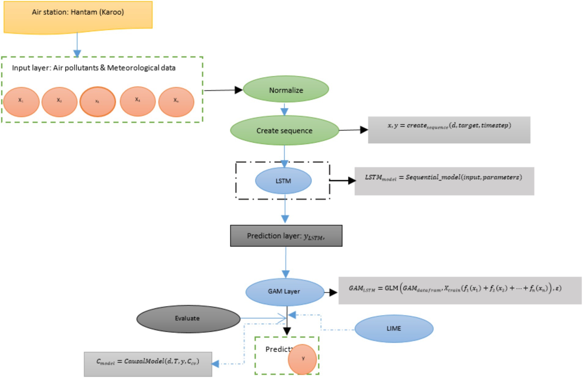
Figure 2. Proposed model.

3.2 Phases of the proposed model

Phases of the proposed model can be expressed as follows:

3.2.1 Dataset

This study leveraged the South African Air Quality Information System (SAAQIS) platform for recent air quality data and reports. Air pollutant data from the Northern Cape National Air Quality Indicator (NAQI) ambient monitoring network from the Hantam (Karoo) station was utilized, focusing largely on the February 2024 pollutant data, which has statistical information such as average, minimum (min) and maximum (max) range for 8-h running average. Statistical information on other features was leveraged from the February 2021 report (that is, CO and WS) and February 2023 (that is, O₃) to augment the February 2024 statistical information. Based on this information, a dataset was synthesized for the city of Kimberley, which contained meteorological and air pollutant concentrations, thereby addressing the data limitation gap. Figure 3 is a map highlighting the location of Hantam and Kimberley, this map was obtained using Python library.

Figure 3

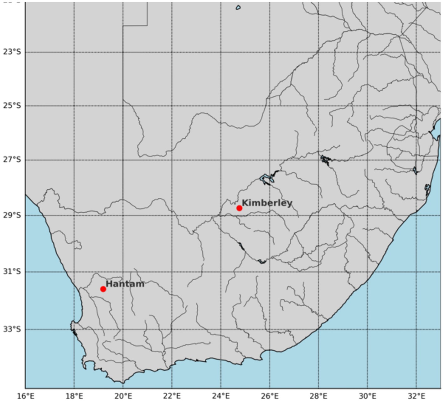
Figure 3. Map of South Africa showing location of Hantam and Kimberley.

3.2.2 Input layer

The synthesized dataset was generated using a random sampling method from a normal distribution, which is bounded by the statistical information like min/max values for each environmental variable and pollutant data from Hantam (Karoo) air monitoring station in Northern Cape Province in the Republic of South Africa. Data was loaded as input into the model for data preparation. The data consists of PM_2.5, PM₁₀, CO, O₃, SO₂, NO₂, NO_x, NO, WS, AT, RH and SR.

Having loaded the data, it is cleansed through data interpolation, then it is normalized and the LSTM sequence is created. Afterwards, it is split into training and test, then loaded into the LSTM model. Data normalization was achieved using the MinMaxScaler method. There were 6,210 instances with 12 features. After normalization, the time sequence is created using the dataset, target and time-step, which is expressed by Equation (1):

$\begin{array}{ll}x,y=\mathit{\text{creat}}{e}_{\mathit{\text{sequence}}}(\mathit{\text{dataset}},\mathit{\text{target}},\mathit{\text{timestep}})& (1)\end{array}$

Where x represents the features and y is the target pollutant, dataset consists of the air pollutants and the target represents what was being predicted. In this regard, the time-step and the features are input into the deep learning time-series models.

3.2.3 Deep learning time-series models

The deep learning models are used to capture the temporal dependencies in the air pollutant concentrations and meteorological variables. The time-series deep learning models considered are LSTM, BiLSTM, GRU, BiGRU, 1DCNN and Transformer. The input features into this layer are of PM_2.5, PM₁₀, CO, O₃, SO₂, NO₂, NO_x, NO, WS, AT, RH and SR. These single models are hybridized with the GAM model to provide a hybrid model for the prediction of CO₂ concentration. These deep learning (DL) models are trained on the original input dataset, and the trained model is used for prediction. DL model is expressed in Equations (2–4).

$\begin{array}{ll}\mathit{LST}{M}_{\mathit{\text{model}}}=\mathit{\text{Sequential}}\_\mathit{\text{model}}(\mathit{\text{input}},\mathit{\text{parameters}})& (2)\end{array}$

$\begin{array}{ll}\mathit{LST}{M}_{\mathit{\text{model}}}=\mathit{LST}{M}_{\mathit{\text{model}}}(x_{\mathit{\text{train}}},y_{\mathit{\text{train}}})& (3)\end{array}$

$\begin{array}{ll}\mathit{LST}{M}_{\mathit{\text{predict}}}=\mathit{LST}{M}_{\mathit{\text{model}}}\left(x_{\mathit{\text{test}}}\right)& (4)\end{array}$

Where $\mathit{LST}{M}_{\mathit{\text{model}}}$ represents the LSTM model and $\mathit{\text{Sequential}}\_\mathit{\text{model}}$ () represents a deep learning library with input and parameters.

3.2.4 Generalized additive model layer

After training the deep learning model to make the predictions, the GAM was used as a post-processing approach to model the relationship between the predictions and actual data, thus allowing for model interpretability and refinement of the predictions. Thus, the generalized additive model is flexible for modeling nonlinear relationships between predictors and the target pollutant. The GAM could be generally expressed in Equations (5, 6):

$\begin{array}{ll}y={\beta }_0+f_1\left(x_1\right)+f_2\left(x_2\right)+\dots +f_n\left(x_n\right)+\epsilon & (5)\end{array}$

Thus,

$\begin{array}{ll}{y}_i={\beta }_0+\sum _{i=1}^{n}f\left(x_i\right)+{\epsilon }_i& (6)\end{array}$

Where y is the predicted air pollutant, $f\left(x_i\right)$ is the nonlinear function (f₁,…,f_n are the smooth functions representing the effect of each predictor like x₁, x₂,…,x_n), β₀ is the intercept term, and epsilon (ϵ) is the error term.

The generalized additive model has a smoothing function that explains each feature’s relation with the target pollutant. For instance, features such as PM_2.5, PM₁₀, SO₂, O₃, NO₂, NOx, WS, AT, RH and SR are the independent variables whereas the target pollutant like NO concentration is the dependent variable which could be explained with GAM in Equation (7).

$\begin{array}{l}\mathit{NO}={\beta }_0+f_1\left(P{M}_{2.5}\right)+f_2\left(P{M}_{10}\right)+f_3\left(S{O}_2\right)+f_4\left(O_3\right)+\\ f_5\left(N{O}_2\right)+f_6\left(\mathit{NOx}\right)+f_7\left(\mathit{WS}\right)+f_8\left(\mathit{RH}\right)+\\ f_9\left(\mathit{AT}\right)+f_{10}\left(\mathit{SR}\right)+\in \end{array}\text{ (7)}$

Again, to predict SO₂, the GAM is expressed by Equation (8):

$\begin{array}{l}S{O}_2={\beta }_0+f_1\left(P{M}_{2.5}\right)+f_2\left(P{M}_{10}\right)+f_3\left({\mathit{NO}}_x\right)+f_4\left(O_3\right)+\\ f_5\left(N{O}_2\right)+f_6\left(\mathit{NO}\right)+f_7\left(\mathit{WS}\right)+f_8\left(\mathit{RH}\right)+\\ f_9\left(\mathit{AT}\right)+f_{10}\left(\mathit{SR}\right)+\in \end{array}\text{ (8)}$

Furthermore, the remaining air pollutant concentrations (PM_2.5, PM₁₀, O₃, NO₂, NO_x) are predicted subsequently to understand the correlation between air pollutant features and a target pollutant. The integration of the LSTM model with GAM was achieved using dataframe, expressed as Equation (9):

$\begin{array}{ll}\mathit{GA}{M}_{\mathit{\text{datafram}}}=(y_{\mathit{\text{test}}},\mathit{LST}{M}_{\mathit{\text{predict}}})& (9)\end{array}$

Thus, $\mathit{LST}{M}_{\mathit{\text{predict}}}$ represent the predictions from the LSTM model and $y_{\mathit{\text{test}}}$ is the test dataset, $\mathit{GA}{M}_{\mathit{\text{datafram}}}$is the dataframe. Generally, the LSTM-GAM model is expressed by Equation (10):

$\mathit{GA}{M}_{\mathit{\text{LSTM}}}=\mathrm{GLM}\left(\begin{array}{l}\mathit{GA}{M}_{\mathit{\text{datafram}}},X_{\mathit{\text{train}}}\left(f_1\right(x_1)+\\ f_2\left(x_2\right)+\dots +f_n\left(x_n\right)\end{array}\right),\epsilon )\text{ (10)}$

Where $f_1\left(x_{1,}\right)$ etc. represent the feature matrix of the training set, $\epsilon$ represents the error term, GLM () is the function to implement the generalized additive model which is important from GLM library, and $\mathit{GA}{M}_{\mathit{\text{datafram}}}$ represents the target air pollutant that is the intercept β₀. Equation (11) was used to fit the model, and Equation (12) was used for prediction.

$\begin{array}{ll}{y}_{\mathit{GAM}\_\mathit{\text{predict}}}=\mathit{GA}{M}_{\mathit{\text{LSTM}}}.\mathit{fit}\left(\right)& (11)\end{array}$

$\begin{array}{ll}{y}_{\mathit{GA}{M}_{\mathit{\text{final}}}}=y_{\mathit{GAM}\_\mathit{\text{predict}}}.\mathit{\text{predict}}\left(x\right)& (12)\end{array}$

Where $y_{\mathit{GA}{M}_{\mathit{\text{final}}}}$ represents the final prediction from the LSTM-GAM. The residual or error term $\epsilon$ was normally distributed using the Gaussian function. The $y_{\mathit{GA}{M}_{\mathit{\text{final}}}}$model was used by the LIME model for interpretation, which is expressed as Equation (13).

$\begin{array}{ll}{A}_{\mathit{\text{LIME}}}=f\left(y_{\mathit{GA}{M}_{\mathit{\text{final}}}}\right)& (13)\end{array}$

Where $A_{\mathit{\text{LIME}}}$represents the LIME explainer, $f\left(y_{\mathit{GA}{M}_{\mathit{\text{final}}}}\right)$ is the function that explains the final predictions to display the output for visualization and causal inference analysis.

3.2.5 Model evaluation metrics

The models were evaluated with mean squared error (MSE), root mean squared error (RMSE) and mean absolute error (MAE). The MSE is expressed in Equation (14).

$\begin{array}{ll}\mathrm{MSE}=\frac{1}{N}\sum _{i=1}^N{(y_i-\overline{y})}^2& (14)\end{array}$

Where $\overline{y}$ is the predicted value from the model, $y_i$ is the actual value of the target pollutant. The interpretation is that a lower MSE value means a better model, and a higher MSE suggest the model is worse. MSE equal to zero means the model’s prediction is perfect. The RMSE is expressed in Equation (15).

$\begin{array}{ll}\text{RMSE}=\sqrt{\mathit{MSE}}& (15)\end{array}$

The MAE is expressed by Equation (16).

$\begin{array}{ll}\mathrm{MAE}=\frac{1}{N}\sum _{i=1}^N(y_i-\overline{y})& (16)\end{array}$

Where $\overline{y}$ is the predicted value of the target pollutant, $y_i$ is the actual value of the target pollutant, and N represents the number of data points.

One of the key methods to evaluate a model is the differences between the actual value and prediction, which should be lower to suggest better prediction, that is, the predicted variable has a value closer to the observed value (Wattal and Singh, 2021). Tian et al. (2023) indicates that when large volumes of data are fed into time-series models for a long-range prediction, their performance is challenged, thus, it is imperative to understand how the model performs to suggest future enhancements.

3.2.6 Post-hoc explanation

Post-hoc explanation explains a decision or prediction of a model. The goal is to interpret the inner workings or the output of a complex model in a simple, human-understandable manner, like linear regression. Thus, it explains how to understand the reason models make certain decisions using an M-day time-step of previous data. These explanations are needed to increase transparency, ensure fairness, improve trust, and satisfy regulatory. In this study, LIME was used to explain the contribution or correlation of each feature in the final prediction. Thus, feature importance and their weighted values are displayed for interpretation. In this regard, to explain the prediction $f\left(x_n\right)$ to a complex model $f$ at each point $x_n$ , the simple linear regression for LIME can be mathematically expressed to approximate $f$ to an interpretable model $g$ within the local neighboring $x_n$ variables by Equation (17).

$\begin{array}{ll}\mathrm{g}\left(\mathrm{x}\right)=arg\underset{g\in G}{min}L(f,g,{\pi }_x)+\delta \left(g\right)& (17)\end{array}$

Where the components $f$is the complex model, $g$ is the interpretable model (that is the linear regression); $L(f,g,{\pi }_x)$ represent the local loss function which measure how well $g$ can approximate $f$ in the neighboring variables $x$ ; ${\pi }_x\left(z\right)$ explains how close sampled points $z$ is to the original point $x$ ; and $\delta \left(g\right)$ is the complexity penalty weight to ensure a simple model. Equations (18–20) represents the mathematical expression.

$\begin{array}{ll}f\left(x\right)=\mathit{LST}{M}_{\mathit{\text{prediction}}}\left(x\right)& (18)\end{array}$

$\begin{array}{ll}g\left(x\right)=w_0+\sum _{i=1}^n{w}_i{x}_i& (19)\end{array}$

$\begin{array}{ll}{\pi }_x=exp(-\frac{D(x,x\prime )}{{\sigma }^2})& (20)\end{array}$

Thus, kernel function computes D, which is the distance between $x$and $x\prime$ ; variance $\sigma$ between $x$and $x\prime$ ; n is the number of features in the matrix; $w_0$is the baseline intercept where the coefficients $w_i$ are the relative importance of each feature.

3.2.7 Causal inference analysis

The causal inference model was leveraged to understand the effect or impact of target air pollutants on predictor pollutants. In this regard, LIME helps to display the features according to their relative importance. The most relevant feature has a higher weighted value, which is then mapped to the target air pollutant using the causal inference model to understand the impact. The other less relevant features are included in the causal inference model as confounding variables (common causes) for a comprehensive mapping. Thus, the causal inference model $C_{\mathit{\text{model}}}$can be expressed by Equation (21):

$\begin{array}{ll}{C}_{\mathit{\text{model}}}=\mathit{\text{CausalModel}}(d,T,y,C_{\mathit{cv}})& (21)\end{array}$

Where d represents dataset, T is the treatment (target pollutant, e.g., $S{O}_2$ ), y is the outcome (e.g., ${\mathit{NO}}_x$ ), and $C_{\mathit{cv}}$ is the common causes, where ${\mathrm{C}}_{\mathrm{cv}}\in [N{O}_2,\mathit{NO},O_3,P{M}_{2.5},P{M}_{10},\mathit{\text{WSpeed}},\mathit{AT},\mathit{RH},\mathit{SR}]$ .

The causal effect is estimated using Equation (22):

$\begin{array}{ll}Y=\mu +\mathit{\gamma T}+\sum _{i=1}^n{\beta }_i{X}_i+\in & (22)\end{array}$

Where $\gamma$ is the approximated or estimated causal effect of T on Y, ${\beta }_i$is the effect of the confounders $X_i$ , $\in$ is the noise (that is, random error term), $\mu$ is the intercept. The terms are $\mu$ intercept term, causal effect treatment term is $\mathit{\gamma T}$ , and $\sum _{i=1}^n{\beta }_i{X}_i$ is the effect of confounder terms, and error term is $\in .$ For each observation y and predicted y, the error term $\in$ is expressed by ${\in }_i=y_i-Y_i.$

3.3 Model parameter description

Table 2 presents the parameter description of the proposed model. The proposed and comparative models were implemented in Python 3.10 due to its programming flexibility, using an Intel Core i3 processor. The relevant deep learning libraries were imported to develop the model. Dropout and regularization was used to avoid overfitting in the deep learning models. Our model training procedure focused on 80% data for training and 20% for testing, while the use of 80% allows sufficient data use for training.

Table 2

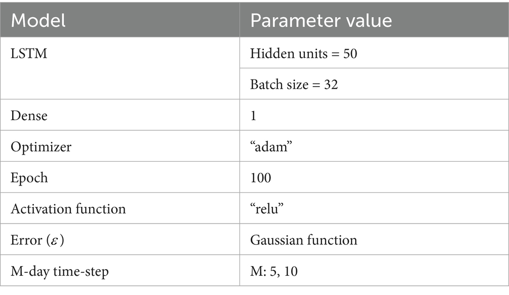
Table 2. Hyperparameter tuning.

The parameter values followed the study by Zhang et al. (2023) on hidden units and epoch, and Hwang et al. (2024) on batch size. Optimizer used is “adam” with relu as the activation function of our proposed model. Furthermore, the random seed control strategy utilized numpy among others which ensures model’s reproducibility during models execution. After completing the 100 epoch, the final model was selected based on the best validation performance.

4 Results

4.1 Models’ prediction over M-day time-step

During the experiment, M-day time-step was considered where M represents the number of previous days data used to train the deep learning time-series models. Table 3 presents the evaluation results of the models prediction with 5-day time-step previous data.

Table 3

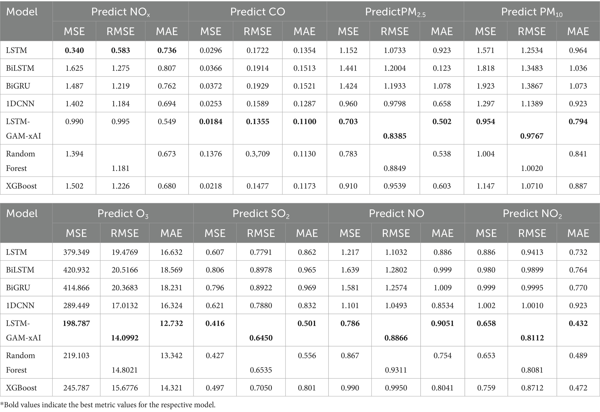
Table 3. Air pollutants predictions with 5-day time-step.

Table 3 shows the 5-day time-step previous of the models to predict air pollutants such as NO_x, PM_2.5, PM₁₀, O₃, SO₂, CO, NO and NO₂. These predictions help in analyzing the predictive performance of each model and comparing it with the proposed model. For instance, in predicting the NOx, it was observed that LSTM, BiLSTM, BiGRU, IDCNN yielded the following MSE values 0.340, 1.625, 1.487, 1.402 and 0.990, respectively, for the deep learning time series models. It emerged that LSTM generated the lowest MSE value of 0.340, while the proposed LSTM-GAM-xAI guaranteed the second least MSE value of 0.990. Comparatively, LSTM-GAM-xAI performed better as it consistently maintained the lowest MSE value in all the air pollutant predictions using the deep learning time-series models.

Again, the two most common machine learning models, such as Random Forest (RF) and XGBoost were also compared with the comparative models. It can be observed that the MSE value for RF is 1.394, and XGBoost guaranteed 1.502. Based on these findings, the proposed LSTM-GAM-xAI guaranteed the least MSE value than the comparative ML models for predicting NO₂ concentration. Furthermore, the proposed LSTM-GAM-xAI guaranteed the best performance across all the air pollutant predictions.

Table 4 shows the statistical information of the LSTM-GAM-xAI model on SO2 predictions for 5-day time-step. It can be observed that, there were 1,237 observation on features. Again, NO₂ had coefficient (coef) of 0.0170 with a constant term ${\beta }_0$ of 1.3411, standard error (std err) of 0.178. Solar radiation had coef of 2.35×10⁻⁰⁵ which is the least among the coefficient values.

Table 4

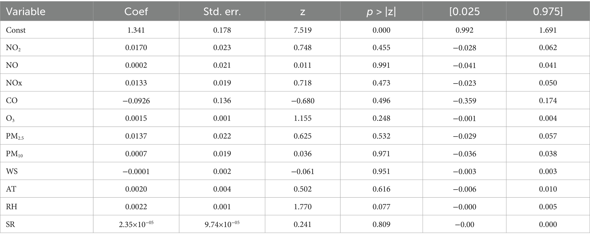
Table 4. LSTM-GAM-xAI statistical information on SO₂ concentration with 5-day time-step.

Based on Table 4, it can be observed that in predicting the target pollutant (SO2), the constant term $({\beta }_0=1.3411),$ NO₂ contributed coef of −0.0170, NO (0.0002), NOx (0.0133), CO (−0.0925), O₃ (0.0015), PM_2.5 (0.0137), PM₁₀ (0.0007), WS (−0.0001), AT (0.0020), RH (0.0022) and SR (2.35e-05). Thus, the general expression can be deduced within the confidence interval (0.025 and 0.975) as follows:

$\begin{array}{l}S{O}_2={\beta }_0-0.0170\cdot \mathit{NO}2+0.0002\cdot \mathit{NO}+0.0133\cdot \mathit{NOx}-\\ 0.0925\cdot \mathit{CO}+0.0015\cdot O3+0.0137\cdot \mathit{PM}2.5+\\ 0.0007\cdot \mathit{PM}10-0.0001\cdot \mathit{WS}+0.0020\cdot \mathit{AT}+\\ 0.0022\cdot \mathit{RH}+(2.35e-05)\cdot \mathit{SR}\end{array}$

Furthermore, Appendix A1 present the detailed statistical information of air pollutants on the 5-day time-step of the previous data considered in this study.

Having experimented the 5-day time-step, further experiment was conducted using 10-day time-step previous data which aimed to further asses the performance of the models. Table 5 shows the 10-day time-step prediction of air pollutants.

Table 5

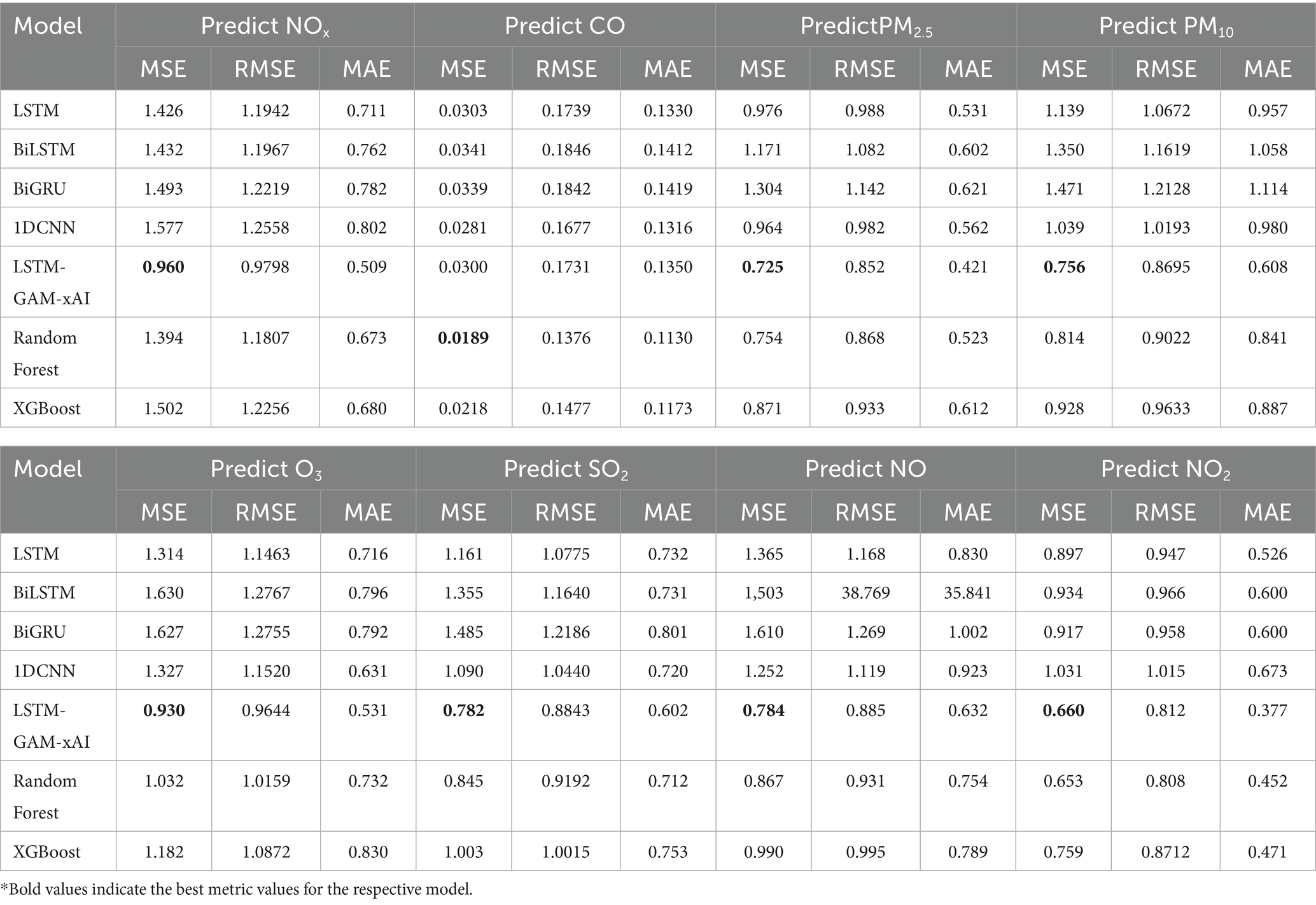
Table 5. Air pollutants predictions with 10-day time-step.

Based on Table 5, it is generally observed that LSTM-GAM-xAI has the best MSE values, in terms of the least MSE value, across the entire prediction of air pollutants. These results suggest that the proposed model performs well given the 10-day time-step previous data.

Table 6 shows the LSTM-GAM-xAI model’s statistical information for the 10-day time-step (e.g., for SO₂ concentration), whereas further statistical information for the remaining air pollutants are shown in Appendix A2. The statistical information includes coef, std err, z and p-value. Where coef represents the estimated coefficient for the predictor pollutants, which is the effect size of how much the outcome changes with an increase in a feature when other features are constant; whereas std err is the standard error, z-score and p-value.

Table 6

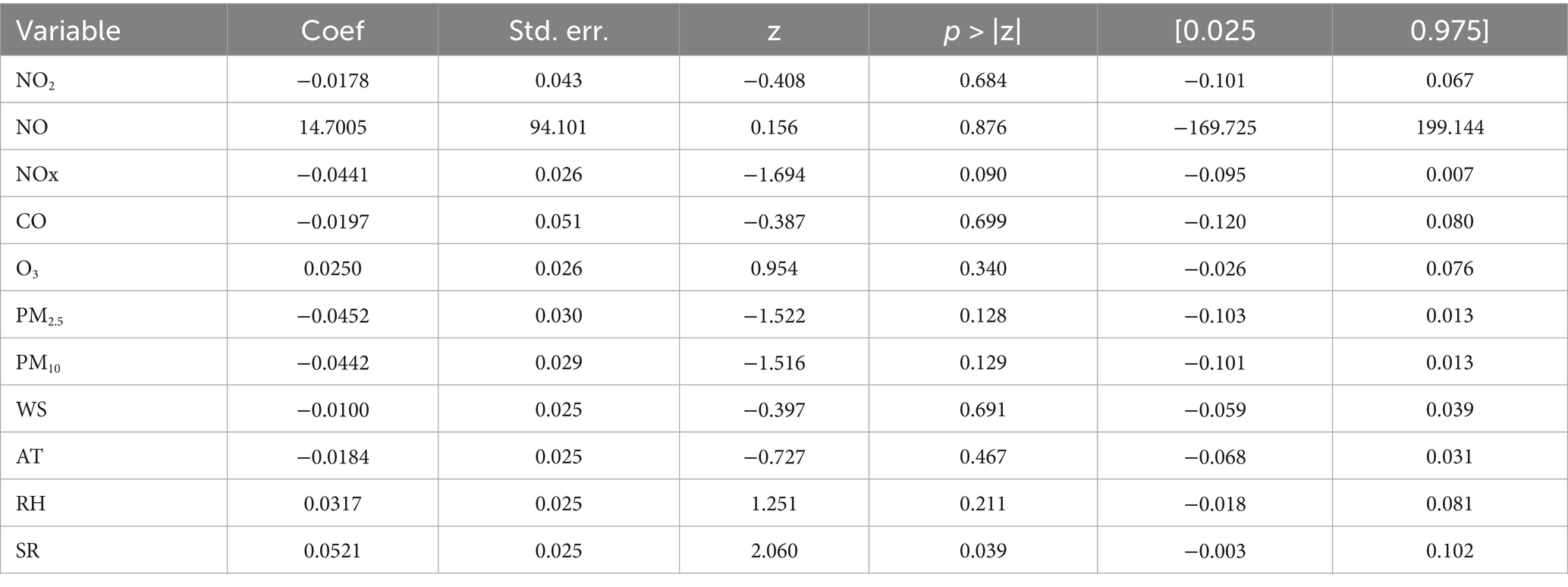
Table 6. LSTM-GAM-xAI statistical information on SO₂ concentration with 10-day time-step.

Based on Table 6, it can be observed that in predicting only SO₂ concentration, NO₂ had coef value of −0.0175, NO (14.7095), NOx (−0.0441), CO (−0.0197), O₃ (0.0250), PM_2.5 (−0.0452), PM₁₀ (−0.0442), WS (−0.0100), AT (−0.0184), RH (0.0317) and SR (0.0521). In view of this, a general expression can be deduced within the confidence interval (0.025 and 0.975) as follows:

$\begin{array}{l}S{O}_2={\beta }_0-0.0175\cdot N{O}_2+14.7095\cdot \mathit{NO}-0.0441\cdot {\mathit{NO}}_x+\\ 0.0250\cdot O_3-0.0452\cdot P{M}_{2.5}-0.0442\cdot P{M}_{10}-\\ 0.0100\cdot \mathit{WS}-0.0184\cdot \mathit{AT}+0.0317\cdot \mathit{RH}+0.0521\cdot \mathit{SR}\end{array}$

4.2 Explainable AI: LIME analysis on LSTM-GAM-xAI model

This section shows the LIME analysis results for only SO₂ concentration within the 5-day time-step and 10-day time-step. While the detail LIME analysis results for the remaining air pollutants are presented in Appendices A3, A4.

Figure 4 shows the LIME analysis results of LSTM-GAM-xAI model focusing on SO₂ concentration within the 5-day time-step. It can be observed that the predicted value lies between min (1.41) and max (1.89) as shown on the horizontal bar, where the intermediate value of 1.63 is the predicted value of the LSTM-GAM-xAI model for the specific instance being explained. Furthermore, the vertical line separates the features into positive and negative ranges. In this regard, features that are located on the positive side such as PM_2.5, CO, AT, and PM₁₀ were the features pushing the prediction toward a 1.63 value.

Figure 4

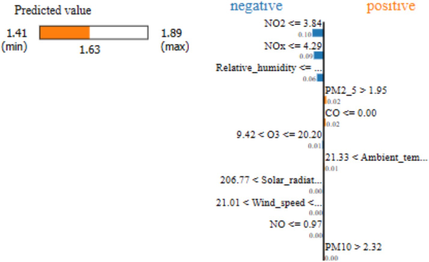
Figure 4. LSTM-GAM-xAI model’s LIME explanation of SO₂ concentration with a 5-day time-step.

Further LIME results of SO₂ concentration in presented in Table 7, focusing on 5-day time-step previous using the LSTM-GAM-xAI model.

Table 7

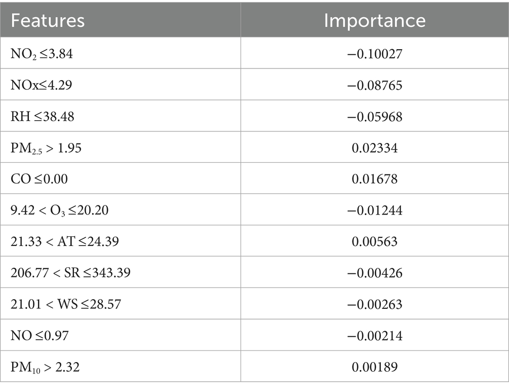
Table 7. LSTM-GAM-xAI model’s LIME explanation for SO₂ prediction with 5-day time-step.

From Table 7, it can be observed that some features recorded negative importance value, such as NO₂, NOx, RH, etc. Other pollutants recorded positive importance value, such as PM_2.5, CO, AT and PM₁₀ in their respective threshold values. “NO₂ $\le$ 3.84” had an importance value of −0.100271, and “PM_2.5 > 1.95” had an importance value of 0.0233407. Where, “PM_2.5 > 1.95” means the PM_2.5 had a threshold value of 1.95 and it contributes positively, a value of 0.0233407, to the prediction of SO₂. Thus, higher PM_2.5 increases the prediction of SO_2, and though the effect is positive, it is relatively weak compared to NO₂ influence on SO₂. Thus, it can be indicated that NO₂ contributed negatively in predicting SO₂ and therefore contributed to pulling down the prediction relative to the local mean. On the other hand, PM_2.5 had a value of 0.0233407, which suggests that PM_2.5 contribute positively to the prediction and therefore pushes the prediction up. Comparatively, PM_2.5 contribute a better positive value as compared with CO (0.0167), PM₁₀ (0.00188). Thus, the simple linear model of LIME can be finally modeled as:

$\begin{array}{l}{g}_{\mathit{\text{LIME}}\_S{O}_2}=w_0-0.10027(N{O}_2\le 3.84)-0.088({\mathit{NO}}_x\le 4.29)-\\ 0.060(\mathit{RH}\le 38.48)+0.023(P{M}_{2.5}>1.95)+\\ 0.017(\mathit{CO}\le 0.00)-0.012(9.42<O_3\le 20.20)+\dots +\end{array}$

In terms of the 10-day time-step to predict SO₂ concentration with the LSTM-GAM-xAI model, the LIME analysis result is presented in Figure 5. It can be observed that “NOx > 400.71” has a feature value approximately −0.07, followed by “O3 $\le$17.11” with a feature value of approx. −0.04. These results suggest that while using the 10-day time-step, previous to predict SO₂ concentration NOx with its threshold value (>400.71) contributed negatively (−0.07) to the prediction of SO₂. Similarly, O₃ with its threshold ( $\le$17.11) also contributed negatively (−0.04) or pulled down the SO₂ concentration. On the other hand, SR ranged between (“342.90 < SR $\le$343.59”) and contributed positively (0.02889) to the prediction of SO₂ concentration. Again, SR was the highest positive feature value among the features recorded during the LIME explanation. Furthermore, the predicted value between the min (−1.06) and max (1.58) is 1.58 as indicated on the yellow bar. This suggests that features that contribute to pushing up the SO₂ are SR, WS, CO, and AT. On the other hand, the features that contribute negatively or push down the prediction are NOx, O₃, NO₂, PM₁₀, RH and PM_2.5.

Figure 5

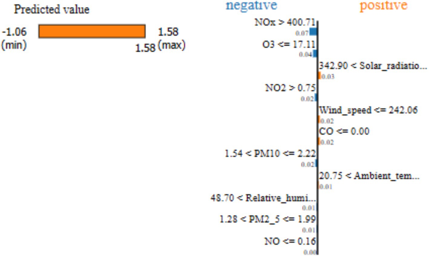
Figure 5. LSTM-GAM-xAI LIME explanation for SO₂ concentration prediction with 10-day time-step.

Furthermore, Table 8 shows the LSTM-GAM-xAI aspect of LIME explanation showing feature importance values for the air pollutants that contributed in SO₂ concentration with 10-day time-step.

Table 8

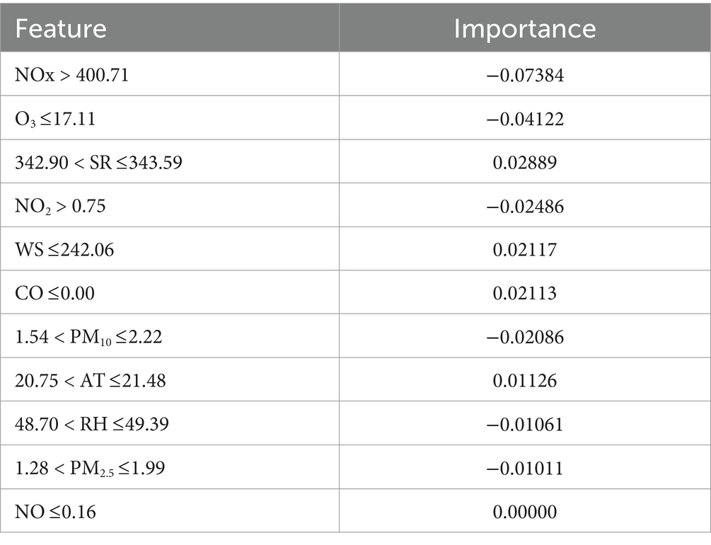
Table 8. LSTM-GAM-xAI LIME feature importance for SO₂ prediction with 10-day time-step.

4.3 Causal inference model

Table 9 presents the causal inference model, which explains the effect or impact of the target pollutant on another. These pollutant features are the features with high relative importance considered as the outcome. Again, other features, with less importance values, were considered confounders in the causal inference model. These features were obtained from the LIME explanation and mapped to the target pollutant. Table 9 presents the causal inference analysis using the 5-day time-step. The analysis is based on components such as estimated effect, new effect and p-value. SO₂, NO, PM_2.5, PM₁₀, O₃ and NO₂ generated estimated effect as 0.002937, 0.008082, −0.004943, −0.003184, −0.003184 and −0.005352, respectively.

Table 9

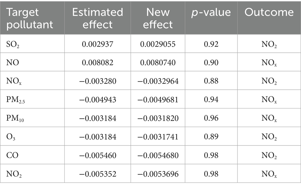
Table 9. Causal inferences analysis with 5-day time-step.

5 Discussion

The experiment results demonstrate different results to help understand the performance of the models (DL and ML) for the air pollutants prediction for the 5-day and 10-day time-steps. Common air pollutants considered are NOx, PM_2.5, PM₁₀, O₃, SO₂, NO and NO₂ with meteorological features. The results indicate that the proposed model demonstrated good performance using the MSE value for 5-day and 10-day time steps. For instance, in predicting SO₂ for the 10-day time-step, the performances are LSTM-GAM-xAI (0.782), LSTM (1.161), BiLSTM (1.355), BiGRU (1.485), 1DCNN (1.090), Random Forest (0.845), and XGBoost (1.003). Again, in predicting SO₂ for 5-day time-step generated the following LSTM-GAM-xAI (0.416), LSTM (0.607), BiLSTM (0.806), BiGRU (0.796), 1DCNN (0.621), Random Forest (0.427), and XGBoost (0.497). These findings suggest that in predicting the hourly concentration level of the air pollutants, the proposed model demonstrated good performance against the comparative models. Huang et al. (2025) combine GAM with eXtreme Gradient Boosting (XGBoost) to predict PM_2.5 concentration in Taiwan with SHAP explanation. Furthermore, He et al. (2023) estimated NO₂ concentration with GAM combined with XGBoost. Cheng et al. (2021) also applied GAM combined with gradient boosting machine (GBM) to determine the relationship between PM_2.5 concentration and environmental factors. In view of this empirical research, GAM has been applied to a machine learning model for air pollutant analysis. Our research also extends the context of research by using the GAM with LSTM and post-hoc explainable artificial intelligence model to provide more explanation on models such as DL and ML models, which are used to predict common air pollutants such as PM_2.5, PM₁₀, SO₂, O₃, NO, NOx, NO₂ using different time-steps.

LIME explanation for SO₂ concentration prediction with a 5-day time-step generated “NO₂ $\le$ 3.84” with importance value −0.10027, “NO_x $\le$ 4.29” with importance value −0.08764, “RH $\le$ 38.48” with importance value −0.05968, etc. (Table 7). Whereas, GAM produced NO₂ with a coefficient (0.0170) followed by NO (0.0002), NOx (0.0133), CO (−0.0925), O₃ (0.0015), etc. (Table 4). It can be observed that the explanation from GAM and LIME placed NO₂ on top of the list of contributing factors in the prediction of SO₂ concentration. These results suggest that on one hand, using LIME, NO₂ contributed −0.10027 to SO₂ prediction. On the other hand, with GAM explanations, NO₂ contributed 0.0170 to the SO₂ prediction. These results indicate that NO₂ pushed up the SO₂ prediction by approximately 0.02 in GAM, while NO₂ reduced the SO₂ prediction by approximately 0.10 in LIME explanation.

The LIME explanation provided the relevant features for the causal inference analysis. The causal effect generated p-value as SO₂ (0.92), NO (0.90), NOx (0.88), PM_2.5 (0.94), PM₁₀ (0.96), O₃ (0.89) and NO₂ (0.98) respectively (Table 9). For instance, in predicting NO concentration, the estimated effect was 0.008082, new effect (0.0080740), p-value (0.90) and outcome (NOx), having confounders as PM_2.5, PM₁₀, SO₂, O₃, NO, NOx, NO_2, RH, AT (Table 8). It is imperative to note that having two air pollutants moving together does not necessarily mean that one variable may have caused another air pollutant to occur. Thus, having determined the causal inference of the air pollutants (Table 8), it could be inferred that not every correlation implies causation; however, every causation implies correlation. Therefore, starting with a correlation analysis involves risks in the case of the proposed model. Thus, another explanation could be as a result of random chance, as the variables may appear to be related, but have no true underlying and clear relationships.

The LSTM-GAM-xAI model produced some detailed statistical information such as the coefficient, standard error, z-score, p-value and confidence interval. Again, number of observations, residual, Pearson Chi-square, etc. (Table 4). The post-hoc explanation model, such as LIME, produced information on features within their threshold, predicted values within a min and max range, and feature values. In view of this, the GAM provides more interpretation than the LIME model. Kaur et al. (2020) indicates that GAM is more interpretable than post-hoc explanation models like SHAP (Kaur et al., 2020). Thus, our study also goes further to suggest that GAM provides more statistical information compared to LIME. Therefore, by proposing and experimenting with the hybrid LSTM-GAM-xAI model for pollutant prediction, detailed information is provided for human understanding. Thus, irrespective of the M-day time steps, our model adapted to the dataset and provided further information on air pollutant analysis for Kimberley.

Though the causal inference model was applied with methodological rigor, the model’s resulting effect estimates (Table 9) produced high p-values (e.g., >0.8) indicating no statistically significant relationships, therefore any conclusion drawn must be interpreted with caution.

While the performance metrics such as MSE, RMSE and MAE provide useful insight, it also emphasizes the baseline to evaluate the technical accuracy of the proposed model in decision making. The interpretability of the output and feasibility of integrating the model in real-world scenarios are essential considerations in assessing whether the model can inform timely interventions in the real world. Although the proposed model achieved relatively low MSE value generally, as compared to the other models, it however shows promising performance results in different time-steps.

Our research contributes in the context of air pollution prediction a transparent and interpretable model that stakeholders could trust. It is worth noting, that researchers have provided several models in different context. For example, Zhu et al. (2024) provided spatio-temporal model based on machine learning for prediction of NO; Lin et al. (2025) incorporated LSTM with GAM and Bayesian model for prediction of different air pollutants; while Goudet et al. (2018) focused on cause-effect inference with the causal generative neural network. The advantage of our model over the existing models is that, ours provide interpretability through the integration of emerging explainable AI model such as LIME with existing GAM and LSTM, thereby bridging the gap between traditional statistical model and deep learning model such as LSTM in a predictive task during environmental monitoring of air pollutants. Furthermore, our model may serve as the alternative to legacy-based air pollutants prediction systems available at air quality monitoring stations in the Northern Cape Province of the Republic of South Africa.

Our proposed model improves interpretability compared to other deep learning models such as LSTM, because it also considered existing statistical models such as GAM, which provides information on coefficient (coef), standard error (std err), z-score, p-value and confidence interval. This information is used by statisticians to understand the behavior of models used in modeling environmental data. Typical LIME or SHAP models lack this information which our model now provides. Therefore, our model provides added value by combining the GAM with post-hoc explanation in terms of transparency and actionable insight for practitioners in environmental monitoring.

6 Methodological limitation

The use of synthetized data based on the measurements from Hantam station for the model evaluation was one of the limitations of this study. As this was due to the lack of air pollutants data for Kimberley. Thus, our research bridges this gap to help evaluate the proposed model’s behavior in a data-scarce context. Again, though using data from one source (e.g., Hantam) to another location (that is, Kimberley) could introduce a potential bias due to site-specific meteorological and geographical differences, this concern was addressed by evaluating the models performance against multiple air pollutants.

7 Conclusion

Air pollutants emission is a global issue as they contribute to global warming and climate-related activities. Human activities like burning fossil fuels contribute to air pollution and climate change. In this study, a deep learning time-series model was proposed that leverages an LSTM model with GAM and offers post-hoc explanation with causal inference analysis of common air pollutants such as PM_2.5, PM₁₀, O₃, SO₂, NO₂, NO, NO_x. Meteorological factors were also considered as input into the proposed model, in addition to these air pollutants. Random sampling method was adopted to synthesis dataset for the City of Kimberley. The local interpretable model-agnostic explanations, which is an artificial intelligence technique, provides a local interpretation of individual predictions. Different time-step previous data, such as 5-day and 10-day, were considered, and MSE, MAE, RMSE values were used to evaluate the predictions. The results indicate better performance value when compared with comparative models. Thus, the study is beneficial to air monitoring stations as it attempts to present alternate models for air pollutant concentration prediction. By conducting this research, we provide an effective approach to assist with the hybridization of the state-of-the-art deep learning time-series model, which could be used as an alternative to a legacy-based air quality prediction model for the city of Kimberley in the Province of Northern Cape, in the Republic of South Africa. Future research should consider the proposed model as one of the emerging models in air pollutant concentration prediction to further fine-tune the predictions in existing real world models.

Data availability statement

The raw data supporting the conclusions of this article will be made available by the authors, without undue reservation.

Author contributions

IA: Writing – original draft, Formal analysis, Methodology, Data curation, Conceptualization, Software, Writing – review & editing. IO: Funding acquisition, Project administration, Validation, Writing – review & editing, Supervision.

Funding

The author(s) declare that financial support was received for the research and/or publication of this article. This work is funded by the Centre for Global Change, Sol Plaatje University, with the National Research Foundation (NRF) (number: 136097).

Conflict of interest

The authors declare that the research was conducted in the absence of any commercial or financial relationships that could be construed as a potential conflict of interest.

Generative AI statement

The authors declare that no Gen AI was used in the creation of this manuscript.

Publisher’s note

All claims expressed in this article are solely those of the authors and do not necessarily represent those of their affiliated organizations, or those of the publisher, the editors and the reviewers. Any product that may be evaluated in this article, or claim that may be made by its manufacturer, is not guaranteed or endorsed by the publisher.

Supplementary material

The Supplementary material for this article can be found online at: https://www.frontiersin.org/articles/10.3389/frai.2025.1620019/full#supplementary-material

References

Adamkiewicz, Ł., Maciejewska, K., Rabczenko, D., and Drzeniecka-Osiadacz, A. (2022). Ambient particulate air pollution and daily hospital admissions in 31 cities in Poland. Atmos. 13:345. doi: 10.3390/atmos13020345

Crossref Full Text | Google Scholar

Agbehadji, I. E., and Obagbuwa, I. C. (2024). Systematic review of machine learning and deep learning techniques for spatiotemporal air quality prediction. Atmosphere, MDPI 15:1352. doi: 10.3390/atmos15111352

Crossref Full Text | Google Scholar

Agbehadji, I. E., and Obagbuwa, I. C. (2025a). Mode decomposition bi-directional long short-term memory (BiLSTM) attention mechanism and transformer (AMT) model for ozone (O3) prediction in Johannesburg, South Africa. Forecasting 7, 1–19. doi: 10.3390/forecast7020015

Crossref Full Text | Google Scholar

Agbehadji, I. E., and Obagbuwa, I. C. (2025b). Integration of explainable artificial intelligence into hybrid long short-term memory and adaptive Kalman filter for sulfur dioxide (SO2) prediction in Kimberley, South Africa. Atmos. 16:523. doi: 10.3390/atmos16050523

Crossref Full Text | Google Scholar

Bai, Y., Ni, Y., and Zeng, Q. (2021). Impact of ambient air quality standards revision on the exposure-response of air pollution in Tianjin, China. Environ. Res. 198:111269. doi: 10.1016/j.envres.2021.111269

PubMed Abstract | Crossref Full Text | Google Scholar

Barbalat, G., Hough, I., Dorman, M., Lepeule, J., and Kloog, I. (2024). A multi-resolution ensemble model of three decision-tree-based algorithms to predict daily NO2 concentration in France 2005–2022. Environ. Res. 257:119241. doi: 10.1016/j.envres.2024.119241

PubMed Abstract | Crossref Full Text | Google Scholar

Becker, D., Alfeus, A., Molnár, P., Boman, J., and Wichmann, J. (2024). Ambient PM2.5, soot, black carbon and organic carbon levels in Kimberley, South Africa. Clean Air J 34:100. doi: 10.17159/caj/2024/34/2.20100

Crossref Full Text | Google Scholar

Bitz, T., Gerling, L., Meier, F., and Weber, S. (2024). Prediction of urban ultrafine particle emission fluxes using generalized additive models. Atmos. Environ. 334:120677. doi: 10.1016/j.atmosenv.2024.120677

PubMed Abstract | Crossref Full Text | Google Scholar

Chang, C.-H., Caruana, R., and Goldenberg, A. (2022). NODE-GAM: neural generalized additive model for interpretable deep learning. USA: Cornell University.

Google Scholar

Charumbira, S., and Ncube, A. (2022). An environmental disaster: a critical review of kimberlite diamond Mining in Kimberley, South Africa. Int J Disaster Risk Reduct :20. doi: 10.2139/ssrn.4232987

Crossref Full Text | Google Scholar

Cheng, M., Fang, F., Navon, I. M., and Pain, C. (2023). Ensemble Kalman filter for GAN-ConvLSTM based long lead-time forecasting. J Comput Sci 69:102024. doi: 10.1016/j.jocs.2023.102024

PubMed Abstract | Crossref Full Text | Google Scholar

Cheng, B., Ma, Y., Feng, F., Zhang, Y., Shen, J., Wang, H., et al. (2021). Influence of weather and air pollution on concentration change of PM2.5 using a generalized additive model and gradient boosting machine. Atmos. Environ. 255:118437. doi: 10.1016/j.atmosenv.2021.118437

PubMed Abstract | Crossref Full Text | Google Scholar

Dammann, L. M., Freitag, M., Thielmann, A., and Säfken, B. (2025). Gradient-based smoothing parameter estimation for neural P-splines. Comput. Stat. 40, 3645–3663. doi: 10.1007/s00180-024-01593-z

Crossref Full Text | Google Scholar

de Asís López, F., Ordóñez, C., and Roca-Pardiñas, J. (2024). A generalized additive model (GAM) approach to principal component analysis of geographic data. Spatial Statistics 59:100806. doi: 10.1016/j.spasta.2023.100806

Crossref Full Text | Google Scholar

de Foy, B., Edwards, R., Joy, K. S., Zaman, S. U., Salam, A., and Schauer, J. J. (2024). Interpretable machine learning tools to analyze PM2.5 sensor network data so as to quantify local source impacts and long-range transport. Atmos. Res. 311:107656. doi: 10.1016/j.atmosres.2024.107656

PubMed Abstract | Crossref Full Text | Google Scholar

Department of Environmental Affairs. (2019). National air quality indicator - monthly data report for the northern Cape Province. p. 1. South Africa. Available at: https://saaqis.environment.gov.za/Pagesfiles/Northern%20Cape%20-%20February%202019.pdf

Google Scholar

Dillon, E., LaRiviere, J., Lundberg, S., Roth, J., and Syrgkanis, V. Be careful when interpreting predictive models in search of causal insights. A joint article about causality and interpretable machine learning with 2018. (2025). Available online at: https://shap.readthedocs.io/en/latest/example_notebooks/overviews/Be%20careful%20when%20interpreting%20predictive%20models%20in%20search%20of%20causal%20insights.html. (Accessed 20 March, 2025).

Google Scholar

Eslami, E., Choi, Y., Lops, Y., and Sayeed, A. (2020). A real-time hourly ozone prediction system using deep convolutional neural network. Neural Comput. & Applic. 32, 8783–8797. doi: 10.1007/s00521-019-04282-x

Crossref Full Text | Google Scholar

Fan, X., Jie, X., Zou, F., Wang, D., da, H., Li, H., et al. (2024). Association between outdoor air pollutants and risk of acute exacerbation of chronic obstructive pulmonary disease in Xi’an, China. Air Qual. Atmos. Health 17, 1373–1390. doi: 10.1007/s11869-024-01513-6

Crossref Full Text | Google Scholar

Fang, C., Zhou, Z., Li, J., Zhou, M., and Chen, X. (2021). Short-term nitrogen dioxide exposure is associated with the spread of S. pyogenes-induced vulvovaginitis in prepubertal girls in Hangzhou, China. Environ. Sci. Pollut. Res. 28, 35790–35797. doi: 10.1007/s11356-021-13268-z

PubMed Abstract | Crossref Full Text | Google Scholar

Forestry Fisheries and the Environment (2024). National air Quality Indicator - monthly data report for the northern Cape Province. South Africa: Department Forestry, Fisheries and the Environment, Republic of South Africa, 1–15.

Google Scholar

Fu, J., Liu, Y., Zhao, Y., Tang, S., Chen, Y., Liu, Y., et al. (2023). Hourly Valley concentration of air pollutants associated with increased acute myocardial infarction hospital admissions in Beijing, China. Atmos. 14:27. doi: 10.3390/atmos14010027

Crossref Full Text | Google Scholar

Fu, G., An, T., Liu, H., Tian, Y., and Wang, P. (2020). Assessment of the impact of PM2.5 exposure on the daily mortality of circulatory system in Shijiazhuang, China. Atmos. 11:1018. doi: 10.3390/atmos11091018

Crossref Full Text | Google Scholar

Gao, A., You, X., Li, Z., Liao, C., Yin, Z., Zhang, B., et al. (2025). Health effects associated with ozone in China: a systematic review. Environ. Pollut. 367:125642. doi: 10.1016/j.envpol.2025.125642

PubMed Abstract | Crossref Full Text | Google Scholar

Goudet, O., Kalainathan, D., Caillou, P., Guyon, I., Lopez-Paz, D., and Sebag, M. (2018). Learning functional causal models with generative neural networks. Xplainable and interpretable models in computer vision and machine learning, 39–80.

Google Scholar

Gu, J., Shi, Y., Chen, N., Wang, H., and Chen, T. (2020). Ambient fine particulate matter and hospital admissions for ischemic and hemorrhagic strokes and transient ischemic attack in 248 Chinese cities. Sci. Total Environ. 715:136896. doi: 10.1016/j.scitotenv.2020.136896

PubMed Abstract | Crossref Full Text | Google Scholar

Habeebullah, T. M. A. (2020). Assessment of ground-level ozone pollution with monitoring and modelling approaches in Makkah, Saudi Arabia. Arab. J. Geosci. 13:1164. doi: 10.1007/s12517-020-06179-9

Crossref Full Text | Google Scholar

Haddad, K., and Vizakos, N. (2021). Air quality pollutants and their relationship with meteorological variables in four suburbs of greater Sydney, Australia. Air Qual. Atmos. Health 14, 55–67. doi: 10.1007/s11869-020-00913-8

Crossref Full Text | Google Scholar

Hammouda, Z., Zaier, L. H., and Blond, N. (2021). Modeling tropospheric ozone and particulate matter in Tunis, Tunisia using generalized additive model. Clean Air J 31, 1–16. doi: 10.17159/caj/2021/31/2.8880

Crossref Full Text | Google Scholar

He, M. Z., Yitshak-Sade, M., Just, A. C., Gutiérrez-Avila, I., Dorman, M., de Hoogh, K., et al. (2023). Predicting fine-scale daily NO2 over Mexico city using an ensemble modeling approach. Atmospheric. Pollut. Res. 14:101763. doi: 10.1016/j.apr.2023.101763

PubMed Abstract | Crossref Full Text | Google Scholar

Huang, C. S., Lo, K., Wu, Y. L., Wang, F. C., Shiu, Y. S., Chen, C. C., et al. (2025). Estimating and characterizing spatiotemporal distributions of elemental PM2.5 using an ensemble machine learning approach in Taiwan. Atmospheric. Pollut. Res. 16:102463. doi: 10.1016/j.apr.2025.102463

PubMed Abstract | Crossref Full Text | Google Scholar

Hwang, J.-S., Gil, J.-W., and Lee, C.-K. (2024). Determination of optimal batch size of deep learning models with time series data. Sustainability 16:5936. doi: 10.3390/su16145936

Crossref Full Text | Google Scholar

Jo, W., and Kim, D. (2023). Neural additive time-series models: explainable deep learning for multivariate time-series prediction. Expert Syst. Appl. 228:120307. doi: 10.1016/j.eswa.2023.120307

PubMed Abstract | Crossref Full Text | Google Scholar

Kaur, H., Nori, H., Jenkins, S., Caruana, R., Wallach, H., Vaughan Wortman, J., et al. (2020). “Interpreting interpretability: understanding data scientists' use of interpretability tools for machine learning” in Proceedings of the 2020 CHI conference on human factors in computing systems (Honolulu HI USA: ACM), 1–14.

Google Scholar

Kruschel, S., Hambauer, N., Weinzierl, S., Zilker, S., Kraus, M., and Zschech, P. (2025). Challenging the performance-interpretability trade-off: an evaluation of interpretable machine learning models. Bus. Inf. Syst. Eng., 1–25. doi: 10.1007/s12599-024-00922-2

PubMed Abstract | Crossref Full Text | Google Scholar

LeCun, Y., Bengio, Y., and Hinton, G. (2015). Deep learning. Nature 521, 436–444. doi: 10.1038/nature14539

PubMed Abstract | Crossref Full Text | Google Scholar

Lin, Y. C., Lin, Y. T., Chen, C. R., and Lai, C. Y. (2025). Meteorological and traffic effects on air pollutants using Bayesian networks and deep learning. J. Environ. Sci. (China) 152, 54–70. doi: 10.1016/j.jes.2024.01.057

PubMed Abstract | Crossref Full Text | Google Scholar

Lou, Y., Caruana, R., and Gehrke, J. (2012). “Intelligible models for classification and regression” in Proceedings of the 18th ACM SIGKDD international conference on knowledge discovery and data mining (Beijing: ACM Press), 150.

Google Scholar

Naz, F., Fahim, M., Cheema, A. A., Viet, N. T., Cao, T. V., Hunter, R., et al. (2024). Two-stage feature engineering to predict air pollutants in urban areas. IEEE Access 12, 114073–114085. doi: 10.1109/ACCESS.2024.3443810

Crossref Full Text | Google Scholar

Nisbet, R., Elder, J., and Miner, G. (2009). “Chapter 7 basic algorithms for data mining: a brief overview” in Handbook of statistical analysis and data mining applications, 121–150.

Google Scholar

Obster, F., Brand, J., Ciolacu, M., and Humpe, A. (2022). Improving boosted generalized additive models with random forests: a zoo visitor case study for smart tourism. Procedia Comput. Sci. 217, 187–197. doi: 10.1016/j.procs.2022.12.214

PubMed Abstract | Crossref Full Text | Google Scholar

Ortega-Fernandez, I., Sestelo, M., and Villanueva, N. M. (2024). Explainable generalized additive neural networks with independent neural network training. Stat. Comput. 34:6. doi: 10.1007/s11222-023-10320-5

PubMed Abstract | Crossref Full Text | Google Scholar

Ravindra, K., Rattan, P., Mor, S., and Aggarwal, A. N. (2019). Generalized additive models: building evidence of air pollution, climate change and human health. Environ. Int. 132:104987. doi: 10.1016/j.envint.2019.104987

PubMed Abstract | Crossref Full Text | Google Scholar

Setianingrum, A. H., Anggraini, N., and Ikram, M. F. D. (2022). “Prophet model performance analysis for Jakarta air quality forecasting” in 2022 10th international conference on cyber and IT service management (CITSM). doi: 10.1109/CITSM56380.2022.9936037

Crossref Full Text | Google Scholar

Sharma, G., Khurana, S., Saina, N., Shivansh,, and Gupta, G. (2024). Comparative analysis of machine learning techniques in air quality index (AQI) prediction in smart cities. Int. J. Syst. Assur. Eng. Manag. 15, 3060–3075. doi: 10.1007/s13198-024-02315-w

PubMed Abstract | Crossref Full Text | Google Scholar

Srivastava, N., Hinton, G., Krizhevsky, A., Sutskever, I., and Salakhutdinov, R. (2014). Dropout: a simple way to prevent neural networks from overfitting. J Mach Learn Res 15, 1929–1958. doi: 10.5555/2627435.2670313

Crossref Full Text | Google Scholar

Talati, I., Shanmugam, R., Shah, K., Chaudhary, N., Parikh, K., and Khaitan, D. (2023). “Air pollution monitoring & prediction system for Ahmedabad region using IOT and ML” in 2023 14th International Conference on Computing Communication and Networking Technologies (ICCCNT).

Google Scholar

Taormina, R., Mesin, L., Orione, F., and Pasero, E. (2011). “Forecasting tropospheric ozone concentrations with adaptive neural networks” in The 2011 International Joint Conference on Neural Networks.

Google Scholar

Tejada-Lapuerta, A., Bertin, P., Bauer, S., Aliee, H., Bengio, Y., and Theis, F. J. (2025). Causal machine learning for single-cell genomics. Nat. Genet. 57, 797–808. doi: 10.1038/s41588-025-02124-2

PubMed Abstract | Crossref Full Text | Google Scholar

Tian, R., Li, X., Ma, Z., Liu, Y., Wang, J., and Wang, C. (2023). LDformer: a parallel neural network model for long-term power forecasting. Front Inform Technol Electron Eng. 24, 1287–1301. doi: 10.1631/FITEE.2200540

Crossref Full Text | Google Scholar

Tu, Q., Hase, F., Chen, Z., Schneider, M., García, O., Khosrawi, F., et al. (2023). Estimation of NO2 emission strengths over Riyadh and Madrid from space from a combination of wind-assigned anomalies and a machine learning technique. Atmos. Meas. Tech. 16, 2237–2262. doi: 10.5194/amt-16-2237-2023

PubMed Abstract | Crossref Full Text | Google Scholar

Tyralis, H., and Papacharalampous, G. (2024). A review of predictive uncertainty estimation with machine learning. Artif. Intell. Rev. 57:94. doi: 10.1007/s10462-023-10698-8

Crossref Full Text | Google Scholar

Wahiduzzaman, M., and Yeasmin, A. (2024). A generalised additive model and deep learning method for cross-validating the North Atlantic oscillation index. Atmos. 15:987. doi: 10.3390/atmos15080987

Crossref Full Text | Google Scholar

Wattal, K., and Singh, S. K. (2021). “Multivariate air pollution levels forecasting” in 2021 2nd International Conference on Advances in Computing, Communication, Embedded and Secure Systems (ACCESS). doi: 10.1109/ACCESS51619.2021.9563281

Crossref Full Text | Google Scholar

Widiputra, H., Mailangkay, A., and Gautama, E. (2021). Multivariate CNN-LSTM model for multiple parallel financial time-series prediction, vol. 54. doi: 10.1155/2021/9903518Citations

Crossref Full Text | Google Scholar

Xiong, K., Xie, X., Huang, L., and Hu, J. (2024). Improved O3 predictions in China by combining chemical transport model and multi-source data with machine learning techniques. Atmos. Environ. 318:120269. doi: 10.1016/j.atmosenv.2023.120269

PubMed Abstract | Crossref Full Text | Google Scholar

Zang, Z., Guo, Y., Jiang, Y., Zuo, C., Li, D., Shi, W., et al. (2021). Tree-based ensemble deep learning model for spatiotemporal surface ozone (O3) prediction and interpretation. Int J Appl Earth Observat Geoinform 103:102516. doi: 10.1016/j.jag.2021.102516

PubMed Abstract | Crossref Full Text | Google Scholar

Zhang, A., Yang, J., and Wang, F. (2023). Application and enabling digital twin technologies in the operation and maintenance stage of the AEC industry: a literature review. J Build Eng 80:107859. doi: 10.1016/j.jobe.2023.107859

Crossref Full Text | Google Scholar

Zhu, Q., Lee, D., and Stoner, O. (2024). A comparison of statistical and machine learning models for spatio-temporal prediction of ambient air pollutant concentrations in Scotland. Environ. Ecol. Stat. 31, 1085–1108. doi: 10.1007/s10651-024-00635-5

Crossref Full Text | Google Scholar

Glossary

xAI - explainable artificial intelligence

LIME - local interpretable model-agnostic explanation

NOx - nitrogen oxides

NO₂ - nitrogen dioxide

NO - nitric oxide

CO - carbon monoxide

O₃ - ozone

PM₁₀ & PM_2.5 - particulate matter

SO₂ - sulfur dioxide

LSTM - long short-term memory model

GAM - generalized additive model

SHAP - Shapley additive explanations

1DCNN - one-dimensional convolutional neural network

BiLSTM - Bi-directional long short-term memory

GRU - gated recurrent unit

ARIMA - autoregressive integrated moving average

CNN - convolutional neural network

LightGBM - light gradient boosting machine

SAAQIS - South African Air Quality Information System

NAQI - Northern Cape National Air Quality Indicator