 Neil Chaudhary
 A. Z. Dhunny
- 1Pangea Society, New Delhi, India
- 2Cyber Analytics, Port Louis, Mauritius
Accurate identification of breast cancer subtypes is essential for guiding treatment decisions and improving patient outcomes. In current clinical practice, determining histological subtypes often requires additional invasive procedures, delaying treatment initiation. This study proposes a deep learning-based model built on a DenseNet121 backbone with a multi-scale feature fusion strategy, designed to classify breast cancer from histopathological biopsy images. Trained and evaluated on the publicly available BreaKHis dataset using 5-fold cross-validation, the model achieved a binary classification accuracy of 97.1%, and subtype classification accuracies of 93.8% for benign tumors and 92.0% for malignant tumors. These results demonstrate the model’s ability to capture morphological cues at multiple levels of abstraction and highlight its potential as a diagnostic support tool in digital pathology workflows.
1 Introduction
Breast cancer remains one of the most prevalent cancers globally, representing a significant health challenge for women across all age groups. According to the World Health Organization (WHO), over 2.3 million women were diagnosed with breast cancer in 2020, making it the most diagnosed cancer worldwide and the leading cause of cancer-related deaths among women (WHO, 2021). The incidence of breast cancer is rising by approximately 3% per year, with higher mortality rates observed in lower-income countries due to limited access to early screening and treatment. In wealthier nations, one in 12 women is diagnosed with breast cancer, whereas in lower-income countries, the rate is one in 27. More concerning is the disparity in mortality: one in 48 women dies from breast cancer in low-income countries compared to one in 71 in high-income countries [World Health Organization (WHO), 2022]. In sub-Saharan Africa, breast cancer now has the highest mortality rate among all cancers affecting women, surpassing cervical cancer. It accounts for 20% of cancer-related deaths in women, with incidence rates varying by region: 30.4 per 100,000 women in Eastern Africa, 26.8 in Central Africa, 38.6 in Western Africa, and 38.9 in Southern Africa. Despite lower incidence rates than in developed countries, the mortality-to-incidence ratio remains alarmingly high at 0.55 in Central Africa, compared to just 0.16 in the United States (GLOBOCAN, 2020).
Early detection has been identified as a critical factor in improving survival rates, with studies showing that early-stage breast cancer has a 90% 5-year survival rate compared to late-stage diagnoses, which can drop to 27% (Siegel et al., 2022). This significant effort is to enhance diagnostic techniques to detect breast cancer earlier and more accurately. Over the past decade, there have been remarkable advances in breast cancer detection, particularly with the integration of advanced imaging techniques and machine learning. Traditional imaging modalities, such as mammography and ultrasound, have been instrumental in identifying breast lesions; however, their sensitivity can decrease in women with dense breast tissue (Kolb et al., 2002). Magnetic resonance imaging (MRI) has emerged as a superior modality for detecting early-stage breast cancer due to its high spatial resolution and ability to differentiate between benign and malignant lesions (Kuhl et al., 2005). Despite its advantages, retention remains complex and prone to variability among radiologists, emphasizing the need for more standardized and accurate approaches. Artificial intelligence (AI) models present a transformative solution to these challenges, especially in resource-limited settings. By leveraging AI to analyze biopsy images, diagnostic accuracy can be improved while reducing the workload of overburdened pathologists. AI-powered systems have demonstrated sensitivities of up to 94.5% in detecting malignant tumors in histopathological images, reducing false-negative rates significantly (Esteva et al., 2021). Additionally, AI-assisted diagnostics have the potential to cut down diagnosis time from weeks to just hours, allowing for earlier treatment initiation and improved patient outcomes. This is particularly beneficial in low-resource settings where a shortage of trained pathologists delays cancer detection (McKinney et al., 2020). By integrating AI into breast cancer diagnostics, healthcare systems in developing countries can bridge the gap in early detection, reduce misdiagnosis rates, and ultimately lower breast cancer mortality. Scalable AI solutions, combined with improved screening programs and public awareness efforts, have the potential to significantly enhance cancer care worldwide.
Despite significant progress in imaging modalities and AI-driven diagnostic tools, most existing models focus primarily on binary classification—differentiating benign from malignant tumors—without addressing the more nuanced and clinically challenging task of histological subtype classification. This limitation hinders their real-world applicability, particularly in cases where treatment decisions depend on precise subtype identification. These gaps underscore the need for a more robust, subtype-aware AI framework trained on whole-slide biopsy images to improve diagnostic granularity and clinical utility.
1.1 Brief review of artificial intelligence in breast cancer
This section provides a brief literature review of what technology has been used for the detection of breast cancer over the past few years for breast cancer detection. And this is going to justify our innovative model and method in the further sections.
AI has revolutionized the healthcare landscape, offering transformative capabilities in automating and enhancing diagnostic processes. In the context of breast cancer detection, AI models have demonstrated superior performance in analyzing complex MRI datasets, identifying patterns that may elude human experts (Lehman et al., 2019). For instance, deep learning convolutional neural networks (CNNs) and attention mechanisms have been applied to segment breast tissues, classify lesions, and predict malignancy with high accuracy (Litjens et al., 2017). These advancements not only reduce errors but also minimize the workload of radiologists, making AI a valuable tool in clinical settings. The integration of AI into breast cancer detection workflows has also been shown to address the challenges of class imbalance and variability in imaging quality. Many studies have employed transfer learning and ensemble techniques to overcome these challenges, achieving higher sensitivity and specificity than traditional methods (McKinney et al., 2020). Moreover, AI-driven algorithms can process datasets quickly and consistently, offering significant advantages in population-based breast cancer screening programs (Rodrigues et al., 2021).
Kaymak et al. (2017) applied neural networks to classify 176 histopathology images, using discrete Haar wavelets for preprocessing. Radial Basis Function Networks outperformed Back Propagation Networks, achieving 70.49% accuracy. Fu et al. (2022) predicted Peripherally Inserted Central Catheter (PICC)-related thrombosis in breast cancer patients using Artificial Neural Network (ANN) and Synthetic Minority Over-sampling Technique (SMOTE) to address class imbalance, outperforming logistic regression (AUC: 0.742 vs. 0.675). Punitha et al. (2021) combined Artificial Immune Systems and Bee Colony optimization for feature selection, improving multilayer perceptron (MLP) performance on the Wisconsin Breast Cancer Dataset (WBCD) dataset for automated diagnosis.
Sharma et al. (2024) used the WBCD to build a stacked ensemble framework integrating Decision Tree, AdaBoost, Gaussian Naive Bayes, and MLP classifiers, achieving 97.66% accuracy. Ensemble learning and feature engineering contributed to its robust performance. Liu et al. (2024a) enhanced a Visual Geometry Group 16-layer network (VGG16)-based model with transfer learning and focal loss to handle class imbalance in 7,841 mammograms, yielding a 96.95% accuracy. Li et al. (2024b) proposed a multimodal fusion model that combined ResNet34-extracted MRI features with RNA-seq gene expression data, using transformers and attention mechanisms to predict treatment response in breast cancer patients more accurately than single-modality approaches.
Munshi et al. (2024) introduced a novel breast cancer detection method by combining an optimized ensemble learning framework with explainable AI (XAI). Using the Wisconsin Breast Cancer Dataset, which contains 32 numerical features, they employed an ensemble model integrating CNNs with traditional machine learning algorithms like random forest (RF) and support vector machine (SVM). U-NET was used for image-based tasks, and a voting mechanism combined RF and SVM predictions. The model achieved an impressive accuracy of 99.99%, surpassing state-of-the-art methods in precision, recall, and F1-score. The integration of XAI enhanced the interpretability and transparency of model decisions, further improving breast cancer diagnostics.
Atrey et al. (2024) developed a multimodal classification system for breast cancer by integrating mammogram (MG) and ultrasound (US) images using deep learning and traditional machine learning techniques. The dataset, sourced from AIIMS, Raipur, India, consisted of 31 patients and 43 MG and 43 US images, which were augmented to 1,032 images. Data preprocessing involved manual region-of-interest (ROI) annotation by radiologists and noise filtering techniques for both image types. The deep learning model, ResNet-18, was used for feature extraction, while SVM classified the fused features. The hybrid ResNet-SVM approach achieved a classification accuracy of 99.22%, significantly outperforming unimodal methods. This study demonstrates the effectiveness of combining deep learning with traditional machine learning for improved breast cancer diagnosis.
Robinson and Preethi (2024) developed the SDM-WHO-RNN model, combining fully convolutional networks with RNNs for classifying 9,109 histopathological images from the Breast Cancer Histopathological Image (BreaKHis) and BH datasets. Preprocessing steps included resizing, noise reduction, and stain normalization, while Least Squares Convolutional Encoder-Decoder (LS-CED) was used for tumor segmentation. The system achieved 97.9% accuracy in detecting complex tumor cells. Zhang et al. (2024) proposed the Convergent Difference Neural Network (V-CDNN), an ensemble of Convergent Difference Neural Networks optimized with a Neural Dynamic Algorithm and softsign activations. Trained on public datasets, the model reached a perfect 100% classification accuracy, demonstrating both speed and robustness.
In their 2021 study, Meha Desai and Manan Shah compared the effectiveness of MLP and CNN for breast cancer detection. The study used datasets such as BreakHis, WBCD, and WDBC, with images and biomarkers preprocessed through normalization and feature extraction (e.g., Discrete Cosine Transform). While both MLP and CNN were trained to classify breast abnormalities, CNN consistently outperformed MLP in terms of accuracy. CNN achieved ~99.86% accuracy on the BreakHis dataset, while MLP’s performance was generally lower. CNN was found to be more reliable for image-based diagnosis, whereas MLP showed limitations for larger datasets.
Further to this, Ezzat et al. (2023) proposed an optimized Bayesian convolutional neural network (OBCNN) for detecting invasive ductal carcinoma (IDC) from histopathology images. This approach integrated ResNet101V2 with Mucinous Carcinoma (MC) for uncertainty estimation. Using the slime mould algorithm to optimize dropout rates, the study fine-tuned the architecture, outperforming other pre-trained networks such as VGG16 and DenseNet121. The model demonstrated significant robustness in diagnosis and generalization. Joseph et al. (2022) proposed a multi-classification approach for breast cancer using handcrafted features, including Hu moments, Haralick textures, and color histograms. These features were combined with deep neural networks trained on the BreakHis dataset. Data augmentation was applied to address overfitting, and a four-layer dense network with softmax activation was employed to enhance classification accuracy.
Paul et al. (2023) proposed a novel breast cancer detection system using an SDM-WHO-RNN classifier combined with LS-CED segmentation. Their approach incorporated preprocessing steps, such as noise elimination and image normalization. The LS-CED segmentation localized nuclei, which were then classified based on size and shape. The system demonstrated high accuracy in detecting cancerous cells. Taheri and Omranpour (2023) introduced an ensemble meta-feature generator (EMFSG-Net) for classifying ultrasound images. Leveraging transfer learning with the VGG-16 architecture, the model employed support vector regression (SVR) to create efficient feature spaces. To address issues like overfitting and dead neurons, the leaky-ReLU activation function was incorporated, leading to improved feature representation and classification performance. Muduli et al. (2021) proposed a deep CNN for automated breast cancer classification using mammograms and ultrasound images. The model, consisting of five learnable layers, employed manual cropping for feature extraction and data augmentation to improve generalization. The approach achieved superior results compared to state-of-the-art methods.
Dr. Suvidha Tripathi’s research contributes significantly to the field of breast cancer histopathology image classification, particularly through innovative approaches that integrate spatial context and hybrid feature representations. In one study, Tripathi et al. proposed a BiLSTM-based patch modeling framework, which treats histopathology image patches as sequential data to capture spatial continuity—an aspect often overlooked in conventional CNNs. This model demonstrated strong performance on the Breast Cancer Histology (Grand Challenge 2018 dataset), highlighting the value of contextual learning in improving classification accuracy. In subsequent work, she introduced a hybrid architecture combining CNNs with Bag-of-Visual-Words (BoVW), effectively integrating handcrafted and deep features to enhance discrimination in limited data settings. This approach outperformed standard deep networks like ResNet and DenseNet on the same dataset, underscoring the benefits of feature selection and hybrid modeling in medical imaging tasks. Together, these studies emphasize alternative paths for improving classification performance—either by modeling inter-patch relationships or by enriching feature spaces—both of which are highly relevant for advancing automated diagnosis in breast cancer histopathology.
This research is toward an innovative approach for breast cancer detection, including the multiple subclasses of breast cancer, which still confuses medical doctors, and it hence makes patients undergo more advanced invasive tests for a better understanding of the disease. The technique is based on an AI model trained on a sizable batch of data. Section 2 discusses the model in detail, Section 3 shows the Results and Discussion, and the Conclusion is given in Section 4.
2 Methodology
This methodology section combines an explanation of the different types of breast cancer and their subclasses, along with an advanced AI technique which has been developed to analyse breast cancer results of biopsy. The aim is, instead of making women go again and again through trial and error with treatments or misdiagnosing the cancer, using AI can make all the difference. As mentioned in the literature review section above, AI tech has changed the way the world views medicine now. Therefore, in this study, we have designed a powerful tool for diagnosing the multiple subclasses. This goes toward a humanitarian cause as women are the target here.
Benign and malignant breast cancers differ in their behavior, prognosis, and treatment approach. Benign tumors, such as fibroadenomas or cysts, are non-cancerous growths that do not invade surrounding tissues or spread to other parts of the body. They tend to have well-defined borders, grow slowly, and usually pose little to no health risk. In contrast, malignant tumors are cancerous and have the potential to invade nearby tissues and metastasize to distant organs through the lymphatic system or bloodstream (Robbins et al., 2010). Malignant breast cancers, such as IDCs, invasive lobular carcinoma (LCs), etc., show uncontrolled cell growth and can require serious medical intervention in the form of surgery and/or radiation therapy. Early identification of a tumour as benign or malignant is critical to deliver appropriate treatment and improve patient health (National Cancer Institute, 2021). In histopathological images, benign and malignant tissues exhibit discernibly unique optical features. Benign tumours present as well-organized structures consisting of cells with uniform shapes, minimal mitotic activity, and intact basement membranes. The stromal and glandular components of benign lesions are usually preserved, showing regular nuclei and minimal pleomorphism. On the other hand, malignant lesions show irregular cellular arrangements, pleomorphic nuclei and frequent mitotic figures (Robbins et al., 2010). They often display disrupted basement membranes and an increased frequency of necrotic regions, further highlighting their aggressive nature. AI image analysis of biopsy images will be able to use these intrinsic differences to ensure earlier and more reliable classification into benign and malignant cases (Rakhlin et al., 2018).
The visual features in the biopsy images provide key characteristics for distinguishing malignant and benign breast tissues. Figure 1a (malignant sample) exhibits irregular, disorganized cell structures with pleomorphic nuclei and a dense, fibrous stroma, indicating uncontrolled cancerous growth. The nuclei appear darker and more varied in shape, with increased mitotic activity and loss of structural integrity (Robbins et al., 2010). In contrast, Figure 1b (benign sample) shows well-organized, rounded glandular structures surrounded by normal fibrous tissue, with uniform cell shapes and minimal pleomorphism (National Cancer Institute, 2021). Both these images have a magnification of 100x.
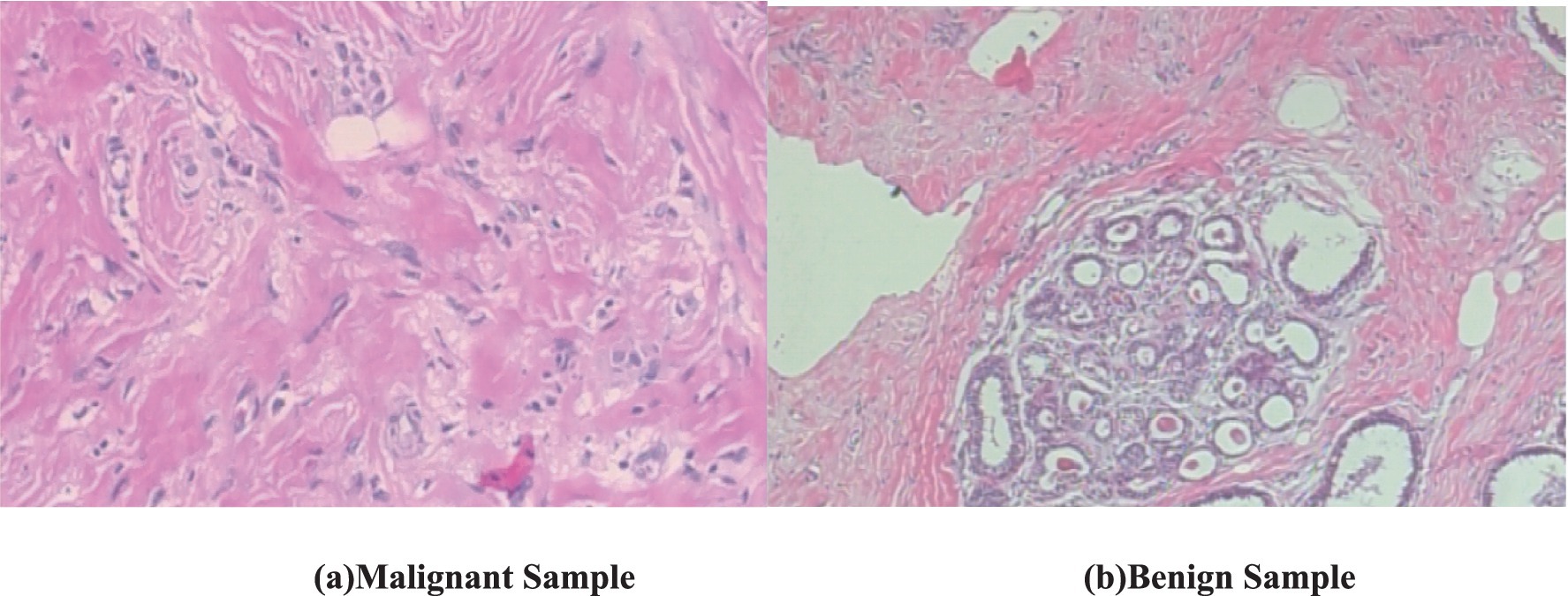
Figure 1. Biopsy image of malignant and benign sample (BreakHis dataset). (a) Malignant sample. (b) Benign sample.
2.1 Dataset
In this study, we utilize the BreaKHis dataset compiled by Spanhol et al. (2016), which contains 9,109 microscopic images of breast tissue captured at four magnification levels: 40×, 100×, 200×, and 400×. These images are categorized into two overarching classes—benign and malignant tumors. Within each class, the dataset further identifies four subtypes: for benign tumors, these include adenosis (A), fibroadenoma (F), phyllodes tumor (PT), and tubular adenoma (TA); and for malignant tumors, ductal carcinoma (DC), LC, mucinous carcinoma (MC), and papillary carcinoma (PC). The image filenames in the BreaKHis dataset encode multiple details about each sample, including the biopsy method used, the tumor’s classification (benign or malignant), its histological subtype, the patient ID, and the magnification level. For instance, the file named SOB_B_TA-14-4659-40-001.png refers to the first image of a benign tumor classified as TA, obtained from patient 14-4659 at a magnification of 40× using the Segmental Orthogonal Biopsy (SOB) technique (Spanhol et al., 2016).
It comprises samples from 82 patients collected at a single institution in Brazil, with no publicly available metadata on age, ethnicity, or receptor status—24 with benign tumors and 58 with malignant tumors. Of the 7,909 images used in the final analysis, 5,429 are malignant and 2,480 are benign, distributed across the aforementioned magnification levels. Following preprocessing and class balancing, the revised class distribution is outlined in Table 1.
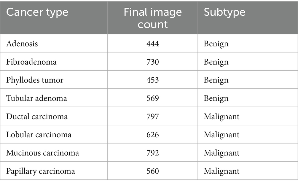
Table 1. Dataset image count for each cancer type.
Benign tumors, by histological standards, lack features associated with malignancy, such as cellular atypia, mitotic activity, invasive growth, or metastatic potential. They typically exhibit localized, slow growth and are considered non-lethal (Robbins and Cotran, 2010). In contrast, malignant tumors are characterized by their capacity to invade neighboring tissues and metastasize to distant sites, often posing life-threatening risks (Robbins and Cotran, 2010). All tissue samples in this dataset were acquired through SOB—a surgical procedure also referred to as partial mastectomy or excisional biopsy. Unlike needle-based techniques, SOB yields larger tissue specimens and is generally performed under general anesthesia in a clinical setting (American Cancer Society, 2019). The classification of tumors into distinct subtypes is based on their cellular morphology under microscopic examination, which holds significance for both prognosis and treatment planning (National Cancer Institute, 2021).
The BreakHis dataset was used for both binary (benign vs. malignant) and multiclass subclass classification. All histopathological images were resized to 128 × 128 pixels and normalized to a standard RGB range. A stratified 80:20 train-test split was employed to preserve class balance across sets. For cross-validation, a 5-fold split was used with data shuffling to ensure unbiased performance evaluation, and no image was shared across folds.
Prior to splitting, real-time augmentation was applied separately to the benign and malignant image sets, increasing the number of benign samples to 7,440 and malignant samples to 9,385. The augmented dataset, totaling 16,825 images, was then split into training, validation, and test sets using a stratified class-wise approach. For both benign and malignant classes, 20% of the data was reserved for testing, and the remaining 80% was further divided in a 75:25 ratio to form the training and validation sets. This resulted in 10,095 images in the training set and 3,365 images each in the validation and test sets.
To improve generalization and address the risk of overfitting due to limited data, we implemented an extensive on-the-fly augmentation pipeline using TensorFlow’s data generators. This included spatial and color transformations to simulate natural histological variation while preserving key tissue features. Table 2 summarizes the augmentation parameters used during training.
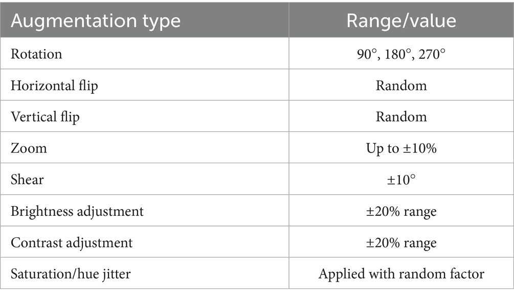
Table 2. Augmentation parameters.
These augmentations were applied to each batch during training to expose the model to diverse variations without expanding the dataset size. In addition, we used early stopping (patience = 5) and ReduceLROnPlateau scheduling to prevent overfitting, along with dropout (0.45), L2 kernel regularization, and batch normalization in each dense layer. Learning curves were generated during each fold to monitor training behavior. The curves showed a minimal gap between training and validation accuracy, indicating stable convergence and effective generalization across classes.
To address class imbalance—particularly for underrepresented subtypes, such as PT and LC—we applied targeted data augmentation during preprocessing. For most classes, each image was augmented using 90° and 180° rotations along with horizontal flipping, effectively tripling their sample size. However, for class label 4 (DC), which was already sufficiently represented, only minimal augmentation was applied to prevent overrepresentation. This strategy helped balance the dataset and reduce bias during training, without altering the loss function or applying weighted sampling.
2.2 Artificial intelligence model
A CNN is a deep learning architecture tailored for grid-like data such as images, leveraging spatial hierarchies to extract local and global features (LeCun et al., 1998). Input images are processed through convolutional layers that apply learnable filters to detect features like edges and textures, generating spatially preserved feature maps (Krizhevsky et al., 2012). Non-linear activation functions, typically ReLU (Glorot et al., 2011), introduce complexity, while pooling layers reduce spatial dimensions and enhance translational invariance (Scherer et al., 2010). Deeper layers capture higher-level abstractions, which are then passed to fully connected layers for classification (Simonyan and Zisserman, 2014). Enhancements such as batch normalization, residual connections (He et al., 2016), and attention mechanisms have further advanced CNN performance, particularly in medical image analysis (see Figure 2).
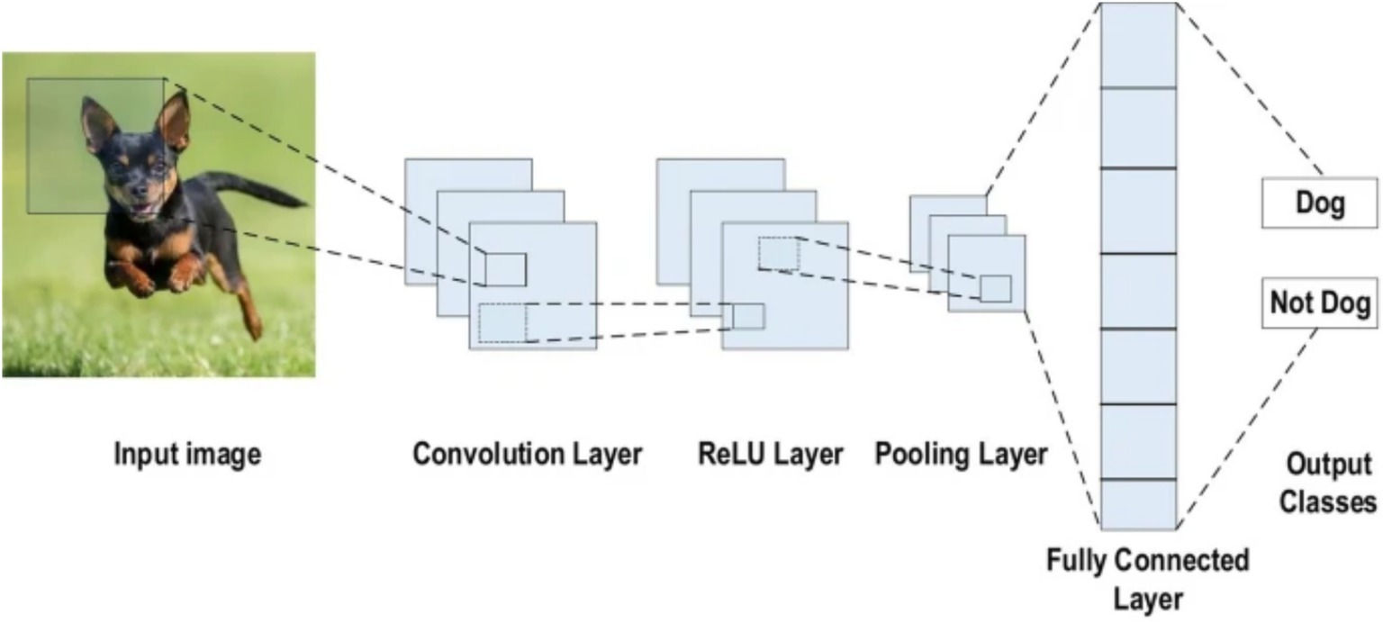
Figure 2. CNN architecture (Alzubaidi et al., 2021).
2.2.1 Classifying images as benign or malignant
In the first approach, a conventional CNN architecture was developed to perform a binary classification of histopathological breast cancer images into benign and malignant categories. Rather than selecting parameters arbitrarily, several architectural configurations were tested iteratively to arrive at a structure that balanced computational efficiency and classification performance. The final model comprised three convolutional layers with 16, 32, and 16 filters, respectively, employing 4 × 4 kernels to effectively capture both low- and mid-level spatial features. This configuration aligns with literature that emphasizes the benefit of using multiple convolutional layers of varying depth for feature extraction in histological images (Spanhol et al., 2016; Bayramoglu et al., 2017). ReLU activation was applied after each convolutional layer to introduce non-linearity, mitigate vanishing gradients, and support efficient learning. MaxPooling layers followed each convolutional block to reduce spatial dimensions and retain salient features (Rakhlin et al., 2018).
The output of the convolutional stack was flattened and passed into a fully connected layer with 256 neurons, enabling high-capacity representation before final classification. A sigmoid-activated output layer was used for binary probability prediction, and binary cross-entropy served as the loss function, both standard choices in binary medical image classification tasks (Gandomkar et al., 2018; Liu et al., 2019). The model was trained using the Adam optimizer (initial learning rate = 0.0001) over 20 epochs, leveraging its adaptive learning rate to ensure stable convergence in a data-limited environment (Bandi et al., 2018). Despite sound architecture and training configuration, this initial model was limited by two key issues: a substantial class imbalance skewed toward malignant samples, and the failure to account for magnification-level heterogeneity across the dataset (40×, 100×, 200×, and 400×). This led to model overfitting, poor generalization, and relatively low accuracy and F1-scores on the validation set. The architectural layout is depicted in Figure 3 (see Table 3).
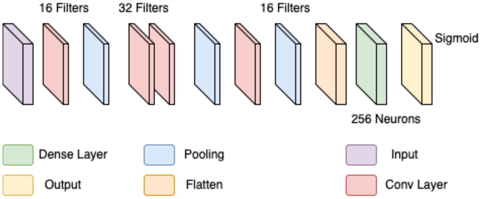
Figure 3. Initial CNN.
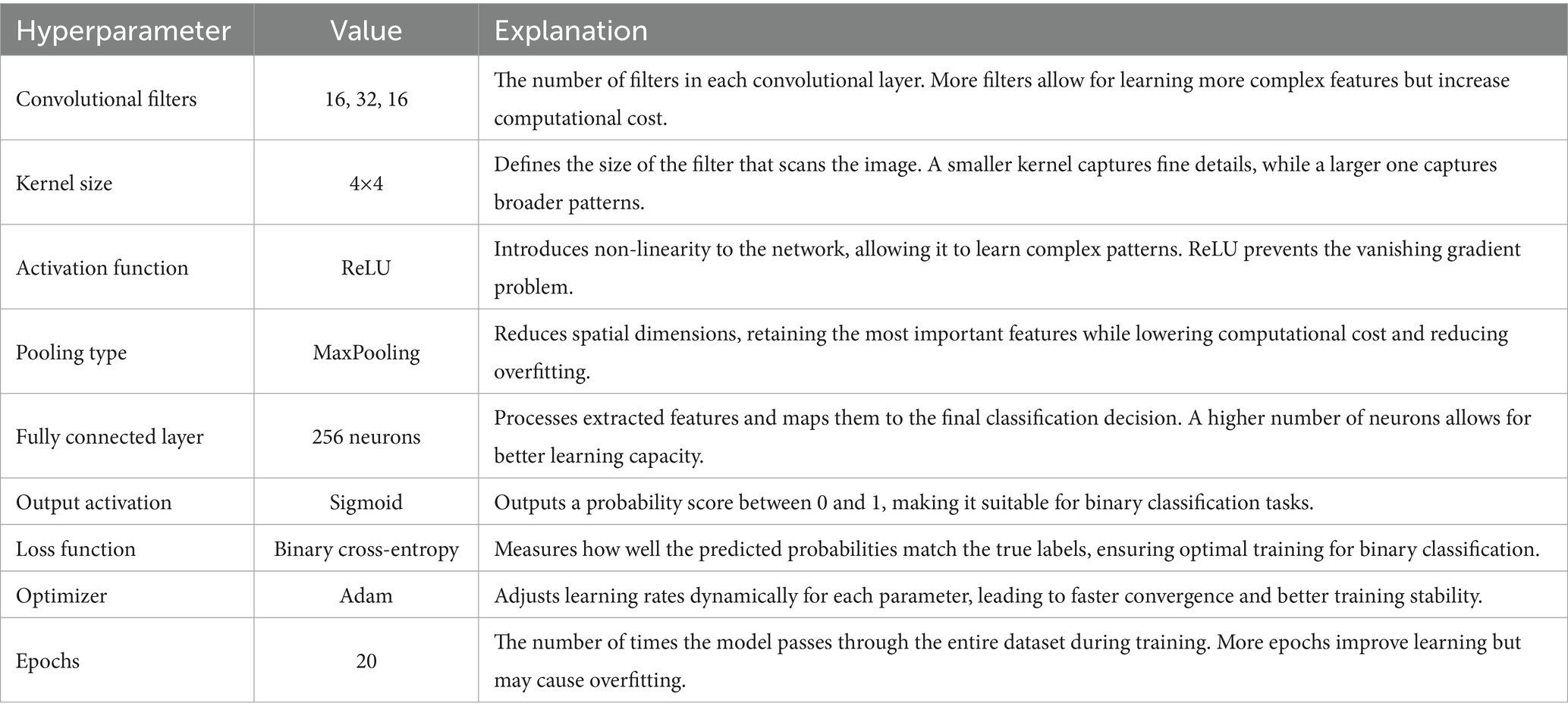
Table 3. Hyperparameters for initial binary classification CNN.
To overcome the limitations of the initial CNN model, a refined approach was adopted, incorporating particle swarm optimization (PSO) for hyperparameter tuning. PSO has demonstrated effectiveness in medical imaging by dynamically optimizing parameters for improved convergence (Houssein et al., 2021). Rather than training a model from scratch, MobileNetV2—a lightweight, pre-trained CNN trained on ImageNet—was employed as a base feature extractor (illustrated by the teal blocks in Figure 4). Transfer learning with pre-trained models has been shown to enhance performance in histopathological classification tasks, especially when annotated datasets are limited (Srinivasu et al., 2021).
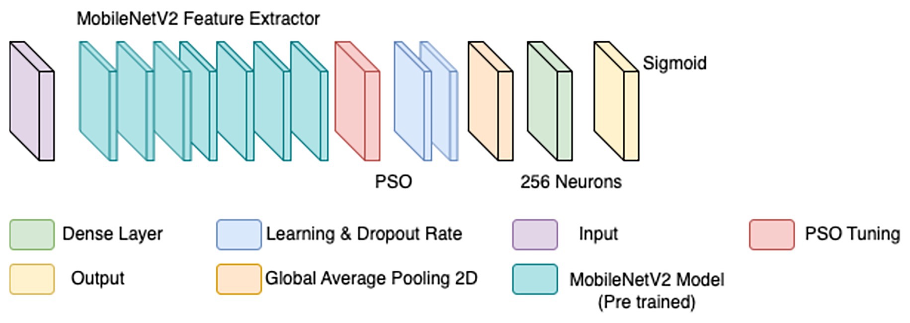
Figure 4. Updated CNN.
The BreaKHis dataset was stratified by magnification level (40×, 100×, 200×, and 400×), and separate models were trained for each resolution, aligning with evidence that such granularity improves classification performance in multi-resolution tasks (Bayramoglu et al., 2017). Within each subset, class balance was ensured by maintaining 250–350 images per class. Data augmentation was applied using ImageDataGenerator, with transformations including rescaling (1./255), width and height shifts (0.2), shear (0.2), zoom (0.2), and horizontal flips. These augmentations were crucial for improving generalization in data-scarce conditions (Bandi et al., 2018).
PSO was used to fine-tune key hyperparameters—specifically, learning rate (searched in the range 1e-5 to 1e-2) and dropout rate (0.3–0.7)—to enhance convergence and prevent overfitting. Optimization was first performed on the 40 × magnification model; the resulting best parameters were then transferred to models for the other magnifications. To further stabilize training, a ReduceLROnPlateau scheduler (factor = 0.5, patience = 3, min_lr = 1e-6) dynamically adjusted the learning rate based on validation loss trends, while EarlyStopping (patience = 5, restore_best_weights = true) halted training when no improvement was observed, thereby avoiding overfitting and saving compute resources (Srinivasu et al., 2021). The final architecture is illustrated in Figure 4. Hyperparameters for this architecture are in Table 4.
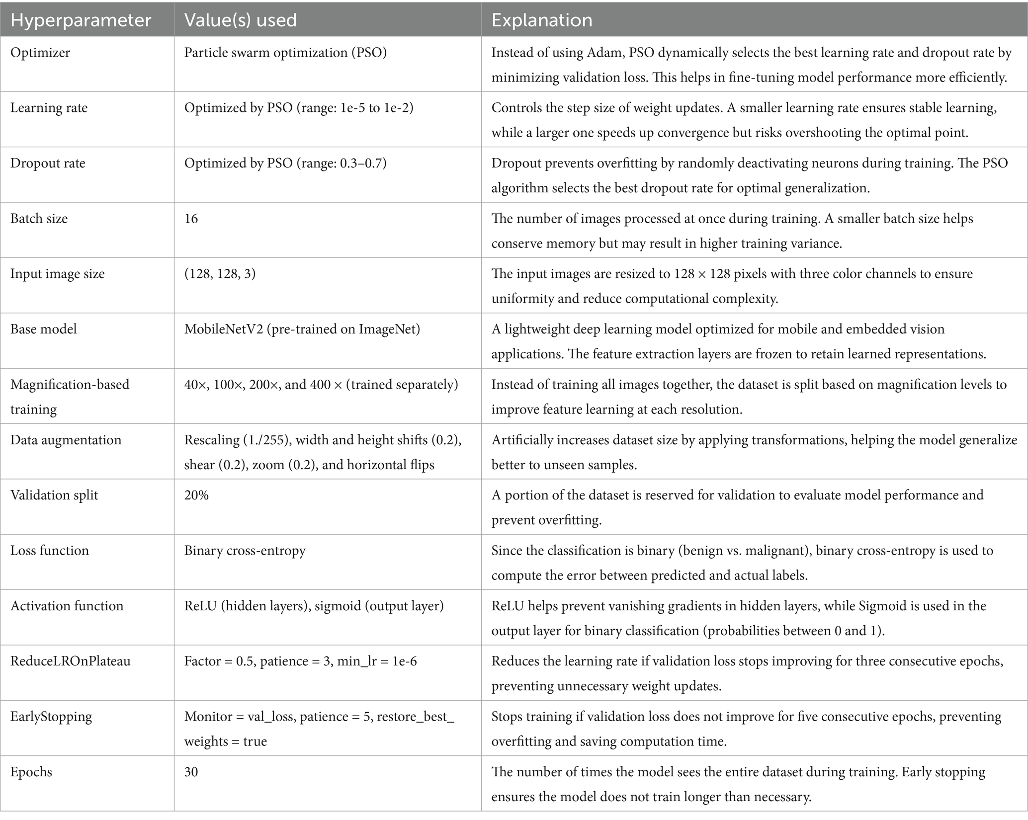
Table 4. Hyperparameters for the first attempt of per-magnification training.
However, this approach too yielded an accuracy far below acceptable levels. F1-scores, recall and precision also hovered around the 50% mark, forcing another change in approach.
The classification of breast cancer histopathology images involved separating the dataset based on different magnification levels (40×, 100×, 200×, and 400×). While this method aimed to leverage magnification-specific features, it resulted in severe dataset fragmentation. Each individual model was trained on a significantly smaller subset of images, which limited the ability to generalize across different test samples. Even with extensive data augmentation, the number of available images remained insufficient, leading to high variance and suboptimal performance during evaluation. Additionally, the previous models relied on relatively shallow CNNs for feature extraction. These networks struggled to effectively capture both low-level and high-level representations within the histopathology images, leading to limited discriminatory power when distinguishing between benign and malignant samples. Given these challenges, a more robust and generalized model was required to improve classification performance across all magnification levels. To overcome the limitations of dataset fragmentation and poor feature extraction, a new model was developed using DenseNet121 as the backbone for feature extraction. DenseNet121, a deep CNN pre-trained on the ImageNet dataset, was chosen due to its efficient parameter utilization and ability to capture intricate hierarchical features. Unlike the previous approach, this model does not separate images based on magnification, allowing for a larger and more diverse training dataset, thereby improving generalization. The proposed model extracts features from three different depths of DenseNet121: conv3_block12_concat, conv4_block24_concat, and conv5_block16_concat. These layers correspond to different levels of abstraction within the network, ensuring that both fine-grained and high-level morphological characteristics are captured. The selection of these layers allows for multi-scale feature extraction, improving the model’s ability to differentiate between benign and malignant samples. The extracted features are processed through a structured pipeline to refine and enhance their representation before classification.
Feature extraction in this model occurred at three levels. The lowest-level feature map, obtained from conv3_block12_concat, captures fundamental visual characteristics such as edges, textures, and color distributions. These features are crucial for identifying initial structural differences in histopathology images, such as variations in cellular arrangements. The mid-level feature map, extracted from conv4_block24_concat, represents more complex patterns, including structural organization within the tissue and variations in gland formation. These features help differentiate between normal and abnormal cellular arrangements. The highest-level feature map, obtained from conv5_block16_concat, provides a more abstract representation, focusing on morphological changes indicative of malignancy, such as nuclear pleomorphism, mitotic activity, and stromal alterations. By incorporating multiple feature extraction levels, the model ensures a comprehensive understanding of tissue characteristics rather than relying on a single-layer representation. To ensure a balance between computational efficiency and adequate feature resolution, an input image size of 128 × 128 was chosen over 256 × 256. While higher resolutions like 256 × 256 could preserve more fine-grained tissue structures, they also significantly increase memory usage and computational load. Given that histopathology images already exhibit high variability and detailed cellular patterns, 128 × 128 provides a sufficient level of detail for feature extraction while allowing for larger batch sizes, faster training, and reduced GPU memory constraints. This choice is particularly important when training multiple models, as excessive computational demands could slow down hyperparameter tuning and optimization.
Each extracted feature map undergoes global average pooling (GAP) to reduce dimensionality while retaining essential spatial information. Unlike max pooling, which selects only the most prominent activations, GAP ensures that all features contribute proportionally to the final representation, enhancing robustness and stability. After pooling, L2 normalization is applied to ensure numerical stability and prevent dominance of certain feature values due to large magnitudes. The normalized feature vectors are then transformed through fully connected layers, where a 64-neuron dense layer introduces non-linearity, allowing for more complex feature interactions. Batch normalization is used to stabilize learning by standardizing feature distributions and improving gradient flow, leading to faster convergence and better generalization. This entire process for one feature is shown by the four blocks in each row in Figure 5. Instead of treating each extracted feature set independently, the model employs a fusion mechanism where feature representations from all three levels are concatenated into a unified feature descriptor (the white block in Figure 5). This approach integrates information across different abstraction levels, allowing the model to make more informed classification decisions. The fused feature vector undergoes further transformation through a dense layer with 16 neurons, refining the representation before classification. To prevent overfitting, a dropout layer with a probability of 0.45 is applied at this stage, randomly deactivating neurons during training and ensuring that the model does not rely on specific patterns that may not generalize well.
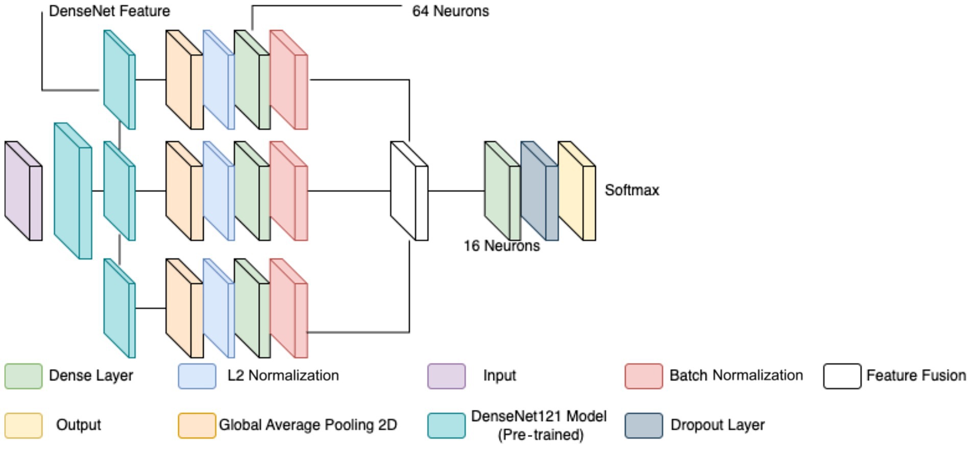
Figure 5. Final binary class CNN.
The final classification layer consists of a softmax activation function with two neurons, representing the benign and malignant classes. This output layer assigns a probability score to each class, allowing for precise decision-making in binary classification tasks. By leveraging deep feature extraction, multi-scale fusion, and regularization techniques, the proposed model significantly improves the accuracy and robustness of breast cancer classification in histopathology images compared to the previous two models, as well as objectively. Figure 5 diagrammatically describes the flow of the updated CNN architecture (see Table 5).

Table 5. Hyperparameters for the final binary classification model.
2.2.2 Classifying images as subtypes of benign and malignant
There are four histologically distinct types of benign breast tumors: adenosis (A), fibroadenoma (F), PT, and TA; and four malignant tumors (breast cancer): carcinoma (DC), LC, mucinous carcinoma (MC) and PC.
Adenosis (A) is characterized by the proliferation of glandular structures, which may appear as distorted acini or ducts in biopsy images. These lesions typically show increased glandular tissue without significant atypia, making them relatively easy to differentiate from malignancies under a microscope (Jiang et al., 2017). Fibroadenomas (F) are solid tumors composed of both glandular and stromal components, presenting as well-circumscribed masses with minimal cellular atypia. Their typical pattern in biopsy images shows a lobular architecture with a fibrous stroma, which contrasts with the irregular structures seen in malignant lesions (Schulz-Wendtland et al., 2016). PTs, though benign in some cases, can show features suggestive of malignancy, such as rapid growth and hypercellularity. Their biopsy images typically display leaf-like structures, hence the name, with prominent stromal overgrowth and areas of necrosis that can challenge differentiation from malignant tumors (Barker et al., 2018). TAs are another benign subtype characterized by well-formed tubules lined by a single layer of epithelial cells. These lesions often have minimal cellular atypia, and their biopsy images demonstrate small, uniformly sized tubules with little stroma (Pike et al., 2020).
In contrast, malignant breast cancers are often more challenging to classify due to the diversity of their histopathological features. DC is the most common type of breast cancer and typically appears as irregularly shaped masses with infiltrating ductal structures. The biopsy images show marked cellular pleomorphism, nuclear atypia, and often necrotic areas, which are indicative of aggressive behavior (Tung et al., 2016). LC presents with a distinctive pattern in biopsy images, with tumor cells growing in a single-file pattern and a lack of cohesive cell groups. This “Indian file” arrangement of cells and the absence of desmoplastic stroma are key features that differentiate it from DC (Vargas et al., 2017). Mucinous carcinoma (MC) is characterized by the production of extracellular mucin, which can be observed in the biopsy images as abundant mucin pools, separating the tumor cells. The cells in mucinous carcinoma are typically round with mild pleomorphism and are surrounded by mucin-rich stroma (Manning et al., 2018). Finally, PC shows prominent papillary structures with fibrovascular cores, surrounded by atypical epithelial cells. The tumor cells are often arranged in well-defined papillae, and the biopsy images reveal a complex architecture with cystic spaces and dense fibrous stroma (Thompson et al., 2019).
A CNN was initially trained to distinguish breast cancer subtypes by learning hierarchical spatial features from biopsy images. It captured architectural differences such as the regular tubules in TAs and the disorganized ductal structures in carcinomas, as well as key histological features like pleomorphism, stromal composition, and mucin presence (Rajendran et al., 2018; Srinivasu et al., 2020). The architecture included three Conv2D layers (32, 64, 128 filters), ReLU activations, and (3 × 3) kernels for efficient feature extraction, with max pooling and dropout (0.25/0.5) to reduce overfitting. A dense layer with 512 neurons and a softmax output layer enabled multi-class classification, optimized using categorical cross-entropy and various learning rates (Adam 0.0001, SGD 0.01, RMSprop 0.0001). Training was conducted over 30 epochs with a batch size of 32. Despite these efforts, the model struggled with generalization and subtype discrimination, yielding poor validation performance. Following the success of the DenseNet-based binary model, the architecture was extended and adapted to a multiclass setting, as detailed in Section 2.3 (see Table 6).
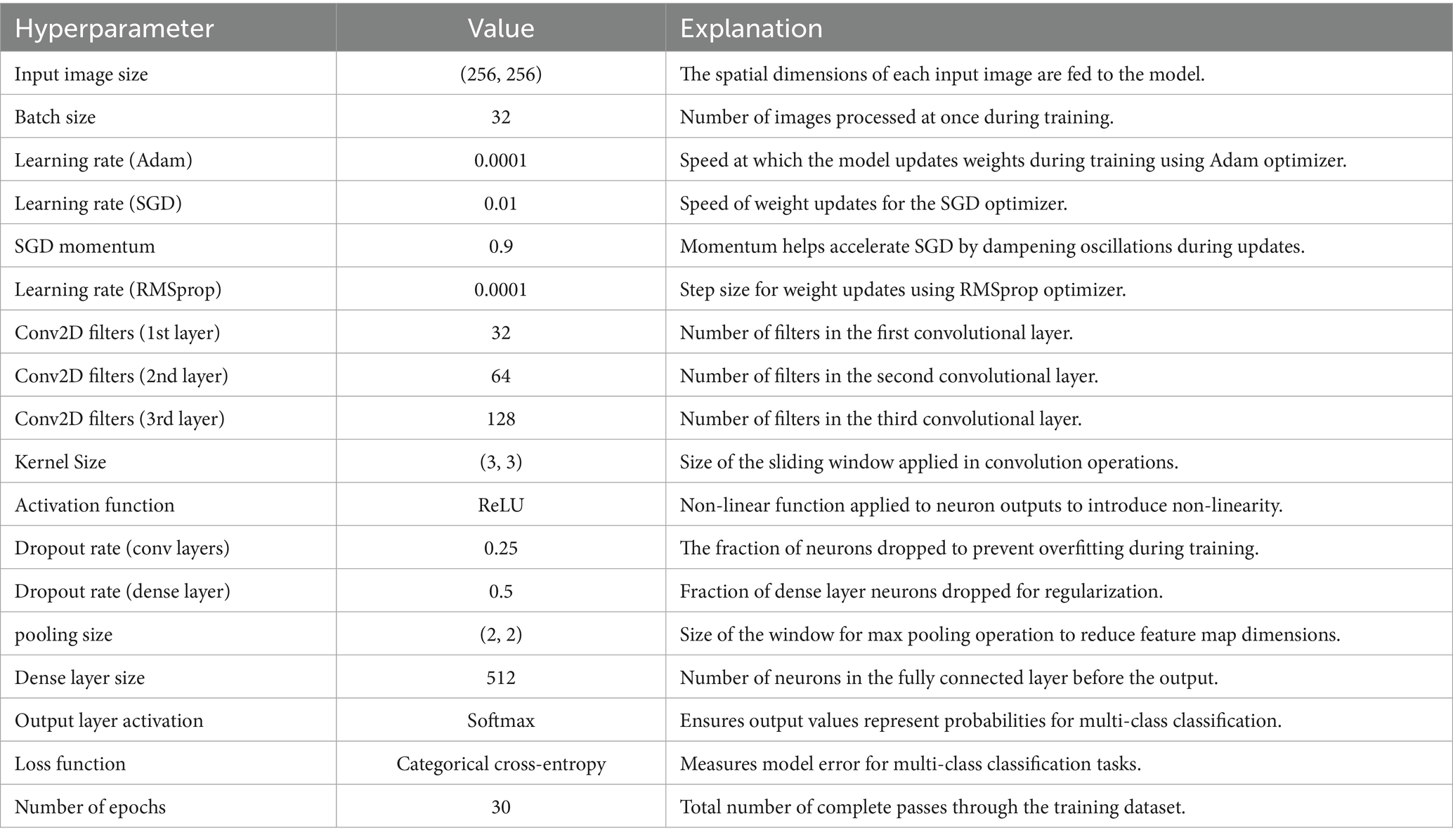
Table 6. Hyperparameters for the initial subclass classification model.
To enhance diagnostic granularity, we developed two separate CNN classifiers—one for benign subtypes and another for malignant subtypes—rather than training a single multi-class model across all categories to extend the binary class classifier to multiple classes. This decision is rooted in both clinical and computational rationale. Clinically, benign and malignant lesions differ not just in severity but in their underlying histomorphological characteristics, tissue organization, and staining patterns (Barker et al., 2018; Pike et al., 2020). Combining both under one classifier risks underrepresenting these distinct patterns during training, especially when using class-imbalanced datasets like BreakHis, which contain fewer samples for certain subtypes. Computationally, separate models allow more focused feature learning within each class family, minimizing intra-class confusion. Prior studies have shown that domain-specific subnetworks often outperform unified multi-class models in pathology, especially when classes exhibit heterogeneity in structure and frequency (Gandomkar et al., 2018; Patel et al., 2024). For example, Umer et al. (2022) observed that a specialized multi-branch CNN improved the classification of individual breast cancer subtypes, while Arevalo et al. (2016) showed that focused lesion-specific training led to better mass detection in mammography. Furthermore, multi-class CNNs trained across all subtypes often suffer from performance trade-offs—gaining sensitivity in one category while losing specificity in others (McKinney et al., 2020). By using separate networks, we achieved higher per-class precision and recall, especially for visually similar classes like fibroadenoma and PT. This modular architecture also supports more targeted clinical applications, such as malignancy-specific triaging or subtype-based treatment suggestion systems, which align with current trends in personalized digital pathology (Lee et al., 2024).
The multi-class CNN architectures for subtype classification were directly adapted from the binary classification model described previously. DenseNet121, used as the backbone in both approaches, provides efficient deep feature extraction through its dense connectivity and hierarchical learning capabilities. As in the binary model, features were extracted from three depths—conv3_block12_concat, conv4_block24_concat, and conv5_block16_concat—capturing progressively abstract morphological features necessary for histopathological differentiation. These include low-level structures such as cellular edges and textures, mid-level patterns like glandular and stromal organization, and high-level attributes such as nuclear pleomorphism and mitotic activity.
Each extracted feature map underwent GAP, L2 normalization, and transformation via a dense layer with L2 regularization, batch normalization, and dropout, following the same processing pipeline outlined in the binary classifier. The processed features were then concatenated into a unified multi-scale descriptor and passed through a final dense layer before classification.
Instead of a binary output, the final softmax layer consisted of four neurons to predict between the benign or malignant subtypes, depending on the network. Two separate CNNs were trained—one for benign subtypes and another for malignant—to reduce feature entanglement and focus each model on intra-class variation. This design choice improved the model’s capacity to learn subtle distinctions specific to each class group, such as distinguishing fibroadenoma from PT, or DC from PC.
Optimization and training procedures mirrored those of the binary classification model, utilizing the Adam optimizer (learning rate 0.0001), EarlyStopping, and ReduceLROnPlateau for improved convergence and generalization (see Figures 6, 7 and Table 7).
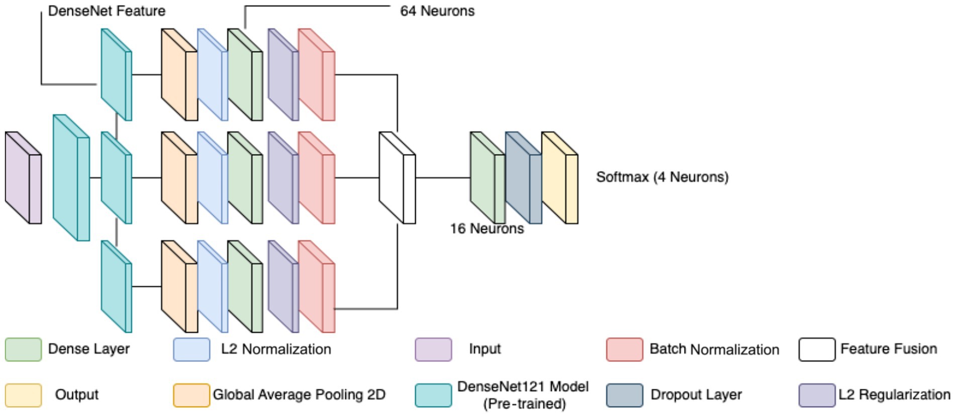
Figure 6. CNN used for multi-class classification.
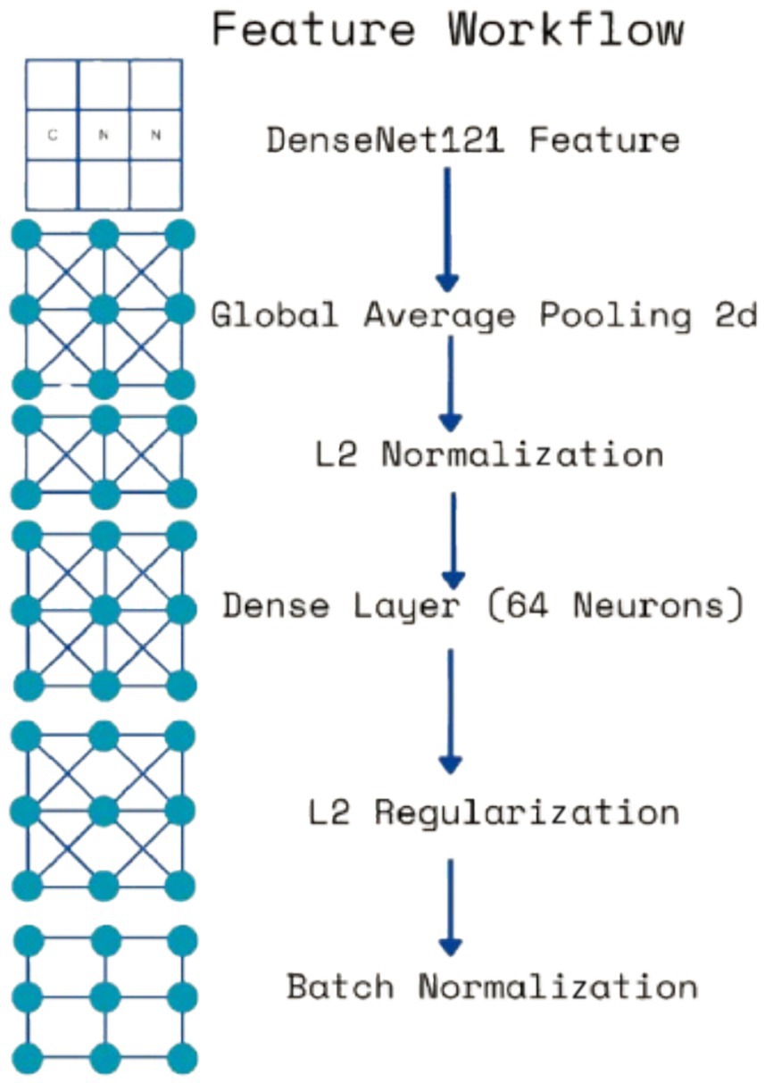
Figure 7. Diagram for feature workflows.
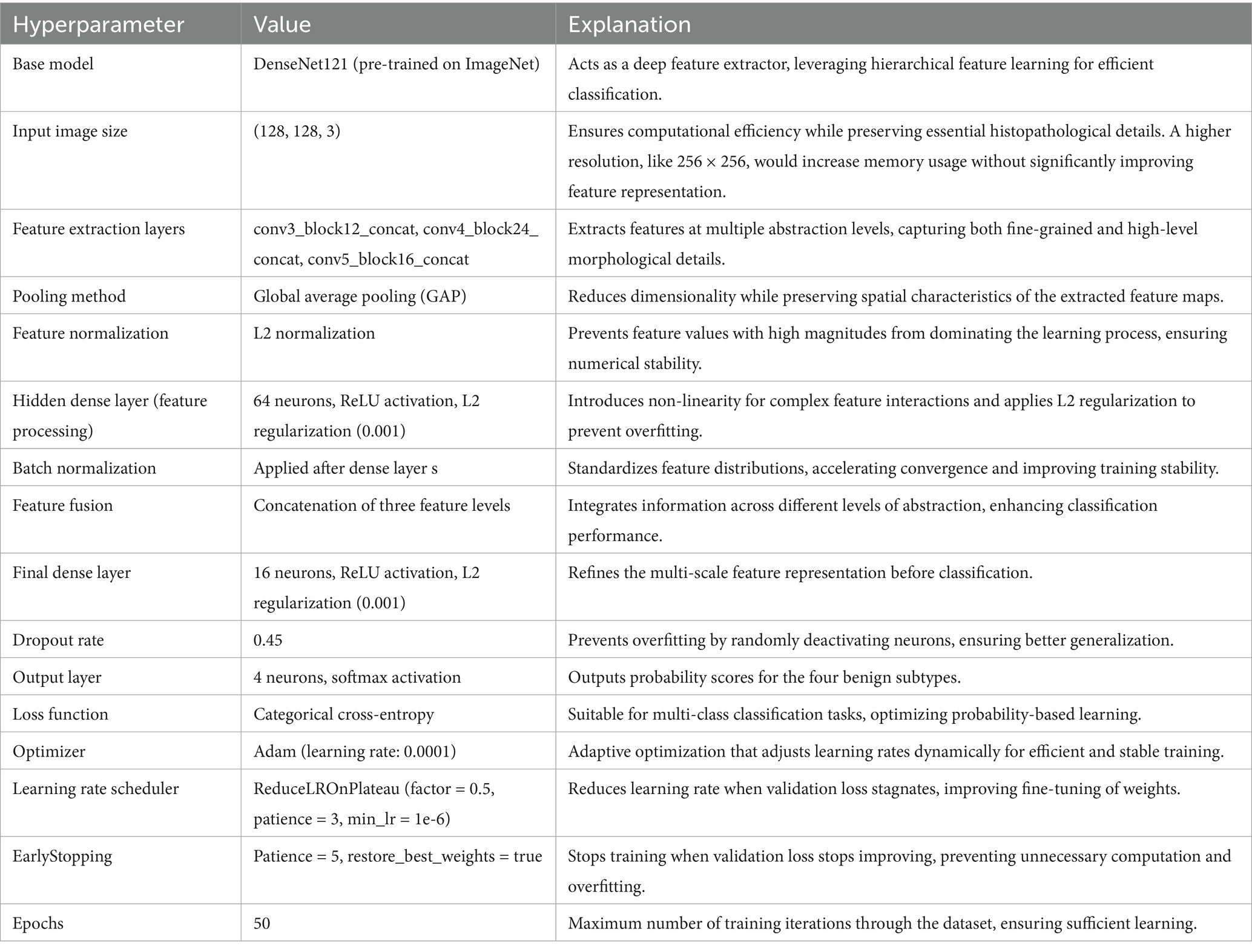
Table 7. Hyperparameters for the final subclass classification model.
2.3 Novel characteristics of the model
The proposed classification algorithm is distinguished by its multi-scale feature fusion architecture built on DenseNet121. Instead of relying only on the final layer features (as done in most standard CNN classifiers), it extracts and fuses features from three different depths of the DenseNet (the end of conv3, conv4, and conv5 blocks). Each feature map is subjected to GAP and L2 normalization, then passed through a small fully connected layer with batch normalization (and dropout) before concatenation. This design enables the model to capture discriminative patterns at multiple spatial scales—from fine-grained cellular details to higher-level tissue organization—within a single network. In essence, the model behaves like an integrated multi-scale ensemble, where lower-level texture features and higher-level semantic features jointly inform the final prediction. This multi-scale fusion is particularly well-suited to histopathology images, where diagnostically relevant cues appear at different magnifications. Prior work has recognized the value of multi-scale information: Araújo et al. (2017) designed a custom CNN to explicitly capture both nuclei-level details and global tissue architecture (Araújo et al., 2017), and Gupta and Bhavsar (2018) similarly argued that “different layers… contain useful discriminative information” for classifying breast histology images (Gupta and Bhavsar, 2018). The proposed model builds on this principle by simultaneously leveraging DenseNet’s intermediate feature maps, rather than using only the deepest features or requiring multiple separate networks.
By fusing intermediate feature vectors, our approach yields a richer representation that combines context from multiple receptive field sizes. This strategy is analogous to the “hypercolumn” or feature pyramid concept—effectively consolidating features at various levels of abstraction. In histopathology, such multi-level fusion has clear advantages: for example, benign vs. malignant differentiation may depend on both cellular morphology and the broader tissue architecture. Traditional transfer-learning classifiers often discard these multi-level cues by only using the final global feature map of a pre-trained CNN. In contrast, our DenseNet121-based model preserves multi-scale feature information by tapping conv3, conv4, and conv5 outputs. Zhu et al. (2019) demonstrated a similar idea with a two-branch “global vs. local” CNN ensemble, where merging a whole-image branch with a high-zoom patch branch improved representation power (Zhu et al., 2019). Our method achieves a comparable multi-scale effect within a single backbone: the conv3_block output (earlier layer) can focus on local textural patterns (analogous to a high-magnification view), while the conv5_block output provides global context (analogous to a low-magnification overview). The DenseNet architecture’s dense connectivity may further facilitate this feature reuse across scales (Huang et al., 2017). Notably, DenseNet121 has been a popular choice in medical image analysis due to its efficient feature propagation; several breast histopathology studies report strong results with DenseNet-based transfer learning—for example, Liew et al. (2021) achieved ~97% accuracy by using DenseNet201 features with an XGBoost classifier (Liew et al., 2021). Our model differentiates itself by not only fine-tuning DenseNet121 on the task, but by modifying its topology to combine multi-scale features—a design rarely explored in prior breast cancer studies.
Another novel aspect of our approach is the use of L2 normalization and balanced regularization in the feature fusion process. Each branch’s pooled feature vector is L2-normalized before fusion, ensuring that no single scale’s features dominate the others due to scale differences. This is an uncommon yet effective practice in classification networks—more frequently seen in metric learning or multi-instance aggregation contexts—and it promotes stability when training the fused classifier. For instance, Xie et al. (2020) applied L2 normalization to patch feature vectors in a histopathology model to stabilize feature magnitudes (Xie et al., 2020). In our design, the L2 norm acts similarly to a scale calibration across the three feature streams, so that the subsequent dense layers operate on features of comparable norm. We then apply dropout and batch normalization in each branch’s dense layer (as well as the final classification layer) to combat overfitting. High-resolution histology images are prone to overfitting given their limited datasets, and regularization is critical. Previous works have indeed found that naive CNN models can overfit histopathology data even with dropout—for example, a shallow CNN still overfit BreakHis patches even with 20% dropout, as reported by Kode and Barkana (2023) (Kode and Barkana, 2023). By combining dropout with batch normalization and the inherent regularization of feature fusion, our model aims to generalize better. The inclusion of batch normalization after the small dense layers also helps each scale-specific feature vector to be well-conditioned before merging, which eases the joint learning. These design choices—L2 normalization of features and dropout-regularized dense layers for each scale—are unique refinements that distinguish our architecture from standard fine-tuned CNN classifiers that often use only a global pooling and a linear classifier on top.
Compared to existing deep learning methods in breast cancer histopathology, the proposed model offers a new balance of simplicity and multi-scale sophistication. Many prior studies have focused either on transfer learning with single CNNs or on ensembles of multiple models. On the one hand, simple transfer-learning approaches, fine-tuning a single network (e.g., ResNet or DenseNet), have shown strong baseline performance (Spanhol et al., 2016; Wahab et al., 2017), but they might miss multi-scale cues. Some recent works augment such models with attention mechanisms—for example, an EfficientNetV2 with a channel-spatial attention module (CBAM) by Aldakhil et al. (2024) outperformed standard CNNs, reaching ~92–94% accuracy on BreakHis magnifications (Aldakhil et al., 2024). Others integrate vision transformers to capture global context—for example, Mehta et al. (2022) introduced a ViT-based HATNet that achieved state-of-the-art accuracy (Mehta et al., 2022). However, these sophisticated models often remain single-scale in the sense that they ultimately rely on one level of feature map (global features) enhanced via attention. On the other hand, ensemble and multi-branch strategies explicitly leverage multi-scale inputs. For example, Umer et al. (2022) proposed 6B-Net, a six-branch CNN with different receptive field sizes in each branch, and fused their outputs for classifying the eight BreakHis classes (Umer et al., 2022). Similarly, an earlier study by Zhu et al. (2019) assembled multiple compact CNNs (and even pruned channels) to combine local and global predictions for histology images (Zhu et al., 2019). These methods confirmed that combining features from multiple scales or multiple models can boost accuracy. Our approach achieves this multi-scale fusion within a single pre-trained DenseNet, rather than requiring separate networks for different magnifications or an external ensemble of classifiers. This provides a more unified and computationally efficient framework: for instance, Wakili et al. (2022) reported a DenseNet-based transfer model (“DenTnet”) that attained ~99% accuracy on BreakHis (Wakili et al., 2022), but that model treats DenseNet as a black-box feature extractor for an SVM or softmax classifier. In contrast, our model integrates the multi-level feature extraction into the training process, which could offer better synergy between feature learning and classification. It also simplifies the pipeline—there is no need for post-CNN classifiers like SVM (as used by Araújo et al., 2017 and others) or gradient boosting ensembles (as in Liew et al., 2021) because the fused deep features are learned end-to-end to directly optimize classification.
In summary, the novelty of our algorithm lies in combining multi-scale feature fusion, transfer learning with DenseNet121, and strategic normalization/regularization into one coherent model for breast histopathology classification. This design captures the multi-scale nature of tissue patterns more explicitly than standard CNN classifiers. It leverages DenseNet’s strength in feature reuse while addressing multiple scales akin to multi-branch networks, but with fewer parameters and a single-pass inference. By comparing with the literature, we see that our approach is unique in how it fuses intermediate CNN features: Gupta and Bhavsar (2018) sequentially processed DenseNet layers’ outputs rather than fusing them, and most other DenseNet-based methods (Wakili et al., 2022; Liew et al., 2021) used only the final layer or combined whole-network outputs in ensembles. Moreover, the inclusion of L2-normalized feature vectors and dropout-regularized dense layers for each scale is a novel architectural choice that, to our knowledge, has not been explicitly reported in prior breast cancer histopathology studies. These innovations position our model as a multi-scale, multi-level classifier that is well-aligned with the visual hierarchy a pathologist employs (from cells to tissue architecture), setting it apart from conventional single-scale CNN models and even from recent attention-based or ensemble-based state-of-the-art methods in this domain.
2.4 Metrics evaluations
In AI, especially in domains like classification and regression, evaluation metrics play a vital role in measuring model performance. Within medical diagnostics, metrics such as precision and recall are particularly significant. Precision reflects the proportion of correct positive predictions, meaning that when a model identifies cancer, it is likely to be correct—thereby reducing unnecessary alarm (Sokolova and Lapalme, 2009). Recall, on the other hand, focuses on identifying as many actual positive cases as possible, which is crucial in healthcare settings to avoid overlooking genuine cases of disease (Sokolova and Lapalme, 2009). Although accuracy is a common metric indicating the percentage of correctly predicted instances overall, it can be deceptive in scenarios with class imbalance, as it does not account for the nature of errors made (Tharwat, 2020).
To address such limitations, the F1-score is often employed. This metric, calculated as the harmonic mean of precision and recall, offers a more balanced view by considering both false positives and false negatives—an essential factor in medical imaging, where failing to detect malignant tumors can have serious consequences (Chicco and Jurman, 2020). Additionally, the area under the curve (AUC) of the receiver operating characteristic (ROC) curve is another key metric. It evaluates the model’s capacity to distinguish between positive (cancerous) and negative (non-cancerous) cases, with scores approaching 1 indicating high discriminative ability (Yang and Ying, 2022). Given the frequent imbalance in medical datasets, relying on a combination of these metrics provides a more reliable and holistic evaluation of model effectiveness (see Table 8).
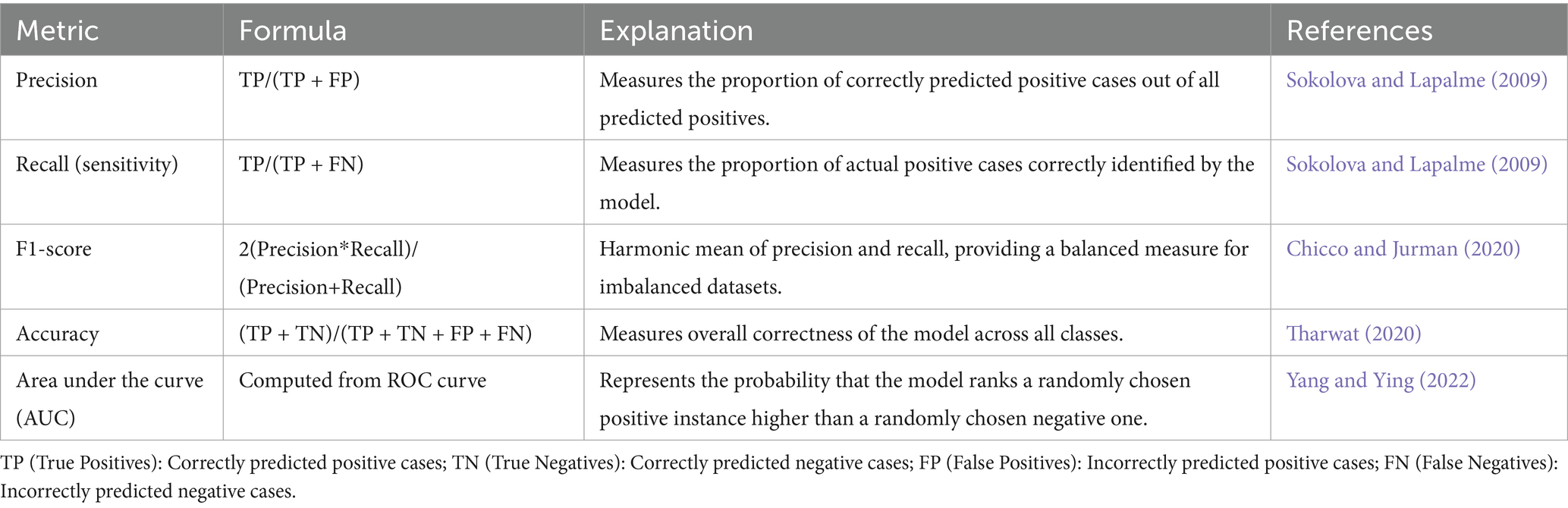
Table 8. Metrics for evaluation of the algorithm.
3 Results and discussion
The following sections present a comprehensive evaluation of the developed AI models across various experimental phases, including binary classification and multi-class subtype detection for breast cancer biopsy images. Detailed performance metrics such as accuracy, precision, recall, F1-score, and ROC-AUC are reported to assess the effectiveness and generalizability of each model. The study began by analyzing the outcomes of the initial CNN architecture, followed by performance improvements observed with the final DenseNet121-based model. It then extends this evaluation to multi-class classification tasks, detailing the results for both benign and malignant subtypes. These results collectively demonstrate the diagnostic power and clinical viability of the proposed framework.
3.1 The binary categorical classification as benign or malignant
The initial CNN architecture, developed for binary classification of histopathology images into benign and malignant categories, was evaluated using different filter and kernel size configurations. Table 9 presented in this section summarizes the performance metrics for each configuration. While the model achieved a maximum accuracy of 84%, this result was below the expected benchmark for binary classification tasks, where an accuracy of 95% or higher is generally required to maintain robust performance during the transition to multi-class classification.
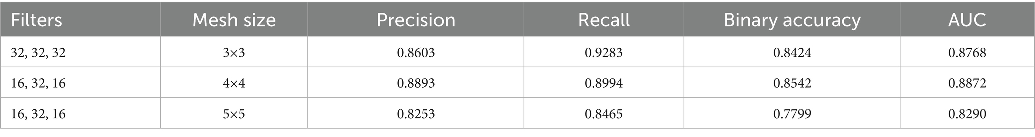
Table 9. Initial results of binary classification.
Upon using the proposed DenseNet121-based binary classification, the model demonstrated outstanding performance in distinguishing between benign and malignant breast cancer histopathology images. The model was trained on out-of-sample biopsy images. As shown in Table 10, the model achieved a test accuracy of 98.63%, indicating a high level of reliability in classification. Precision, recall, and F1-score values were also notably high at 0.9888, 0.9867, and 0.9877, respectively, reflecting the model’s ability to correctly identify malignant cases while minimizing false positives and false negatives. The ROC-AUC score of 0.9863 further confirms the model’s strong discriminative capability, showing its robustness in distinguishing between the two classes across different classification thresholds. Figure 8 shows the confusion matrix for the classification, while Figure 9 is a graph showing the change in accuracy and loss with respect to epochs. Compared to previous models that relied on shallow convolutional architectures and dataset fragmentation based on magnification levels, the proposed model benefits from multi-scale feature extraction at different network depths, improving its ability to generalize across varying histopathological patterns. By utilizing a 128 × 128 input image resolution, the model strikes a balance between computational efficiency and feature preservation, allowing for optimal learning without excessive memory consumption. The use of feature fusion across different abstraction levels enhances the classification robustness, ensuring that both low-level structural features and high-level morphological variations contribute to the final decision-making process.
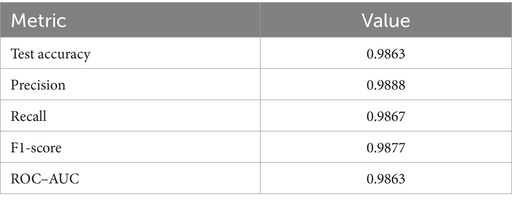
Table 10. Final results of binary classification algorithm.
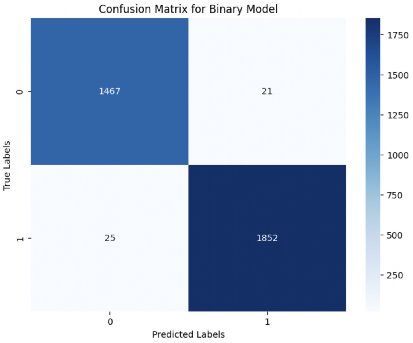
Figure 8. Confusion matrix for final binary classification.
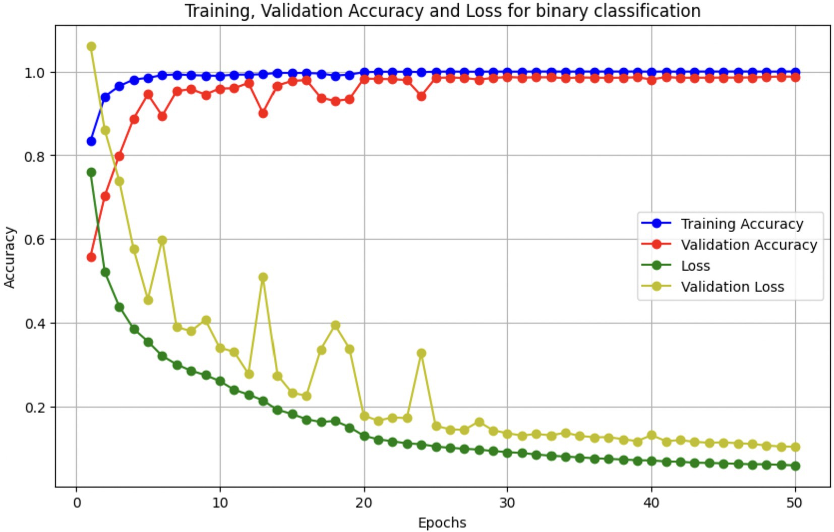
Figure 9. Accuracy/loss vs. epoch graph.
3.2 Multi-category classification of benign and malignant cancers
The performance of the multi-class classification models for benign and malignant breast cancer subtypes is summarized in Table 11. The model was trained on out-of-sample biopsy images. The model trained for benign classification achieved a test accuracy of 0.9382, whereas the malignant classification model obtained a test accuracy of 0.9158. Additionally, the malignant model demonstrated strong predictive capabilities, with a precision of 0.9151, recall of 0.9240, and an F1-score of 0.9182, while the benign model had a precision of 0.9541, recall of 0.9324 and an F1-score of 0.9415. These results highlight the effectiveness of using separate CNNs for each subtype, allowing for improved feature extraction and discrimination between fine-grained morphological variations. Figure 10 shows the confusion matrix for the benign model, while Figure 11 shows the same for the malignant model. Figure 12 shows the graph of the change in accuracy/loss with respect to the epochs for benign, and Figure 13 shows the same for malignant.
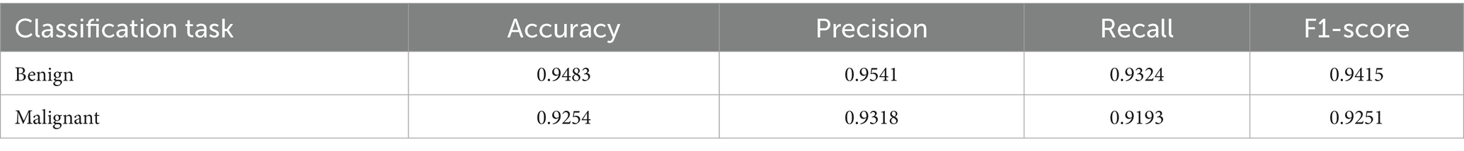
Table 11. Final results for multi-category classification.
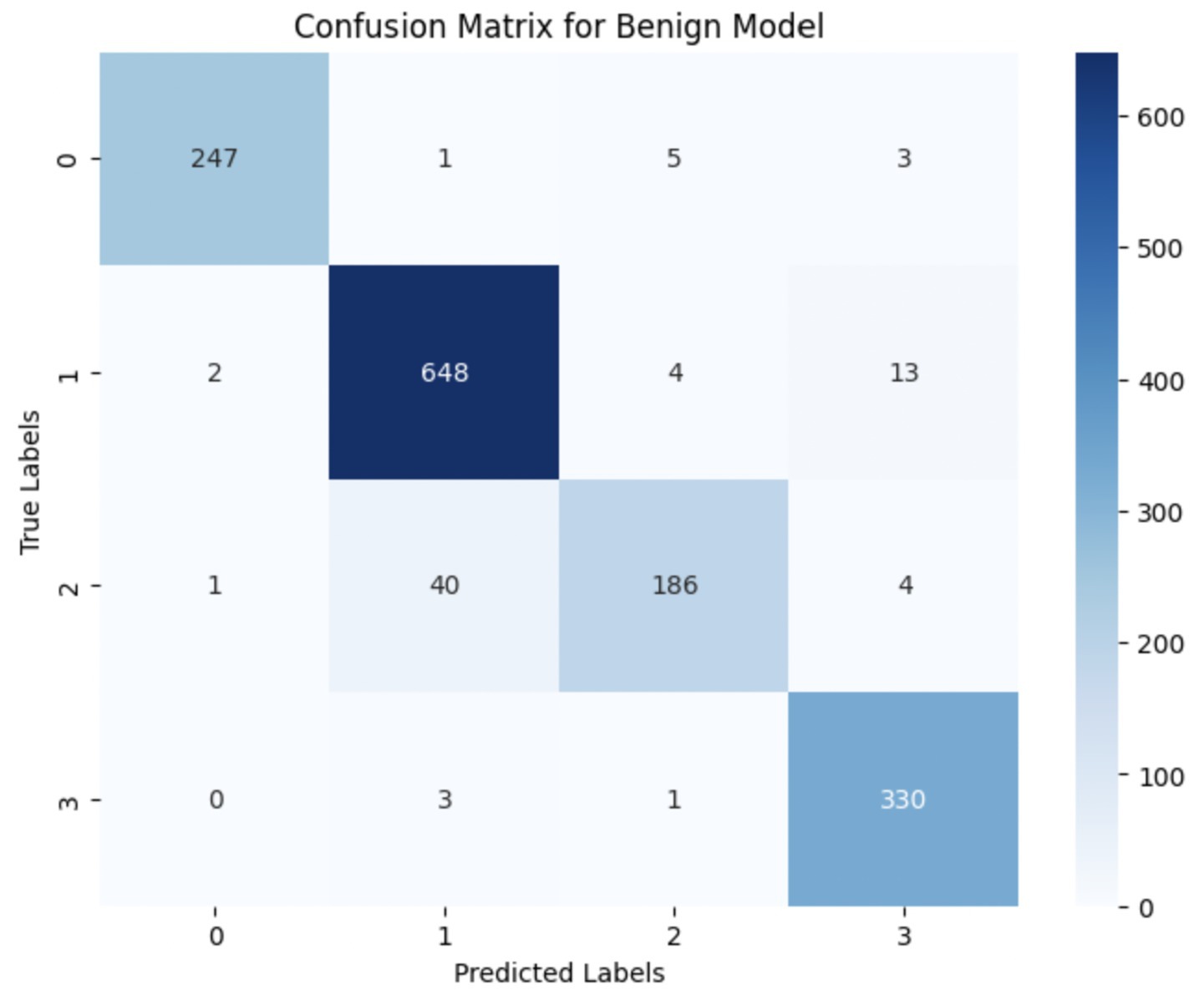
Figure 10. Confusion matrix for benign sub-category classification.
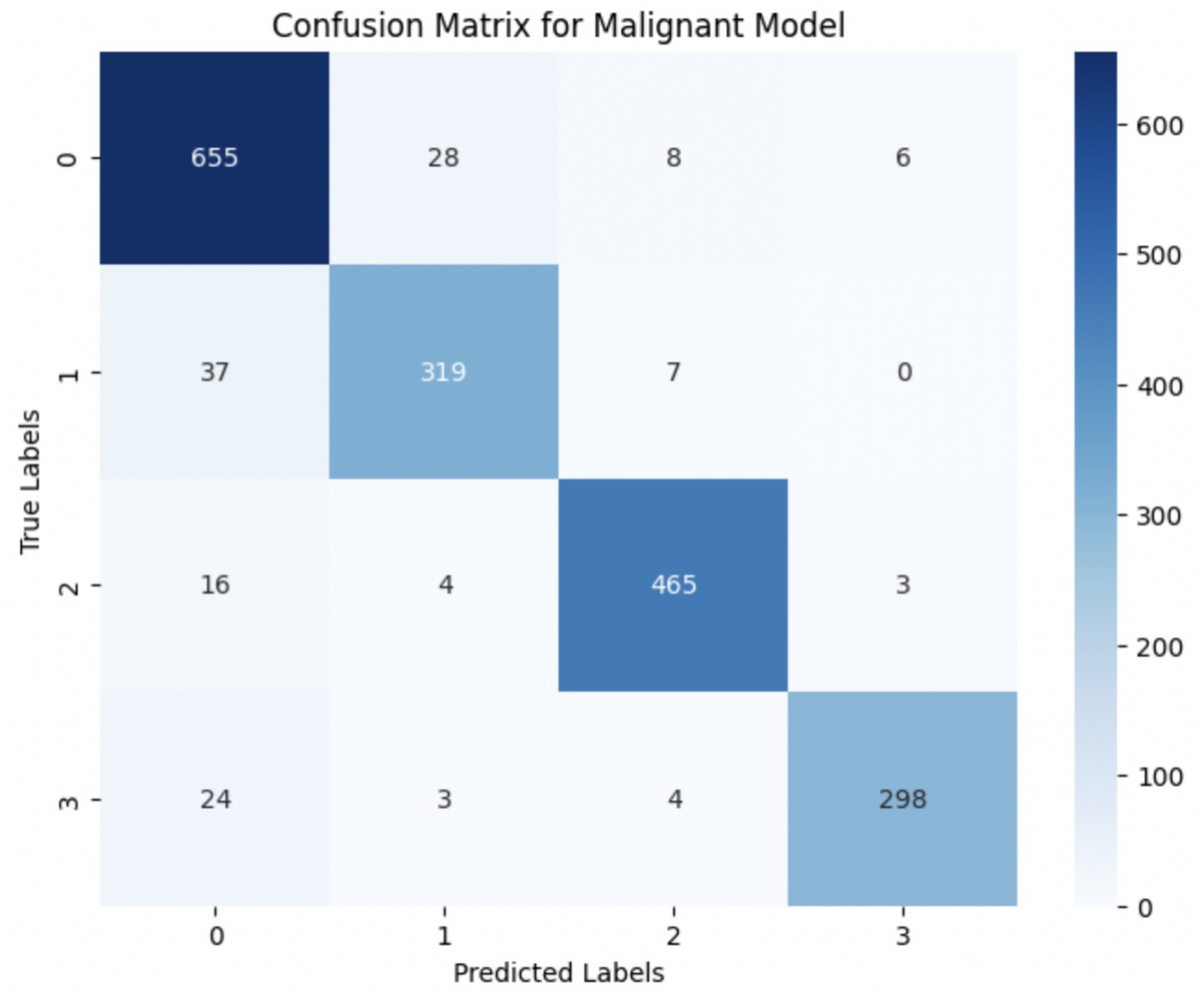
Figure 11. Confusion matrix for malignant sub-category classification.
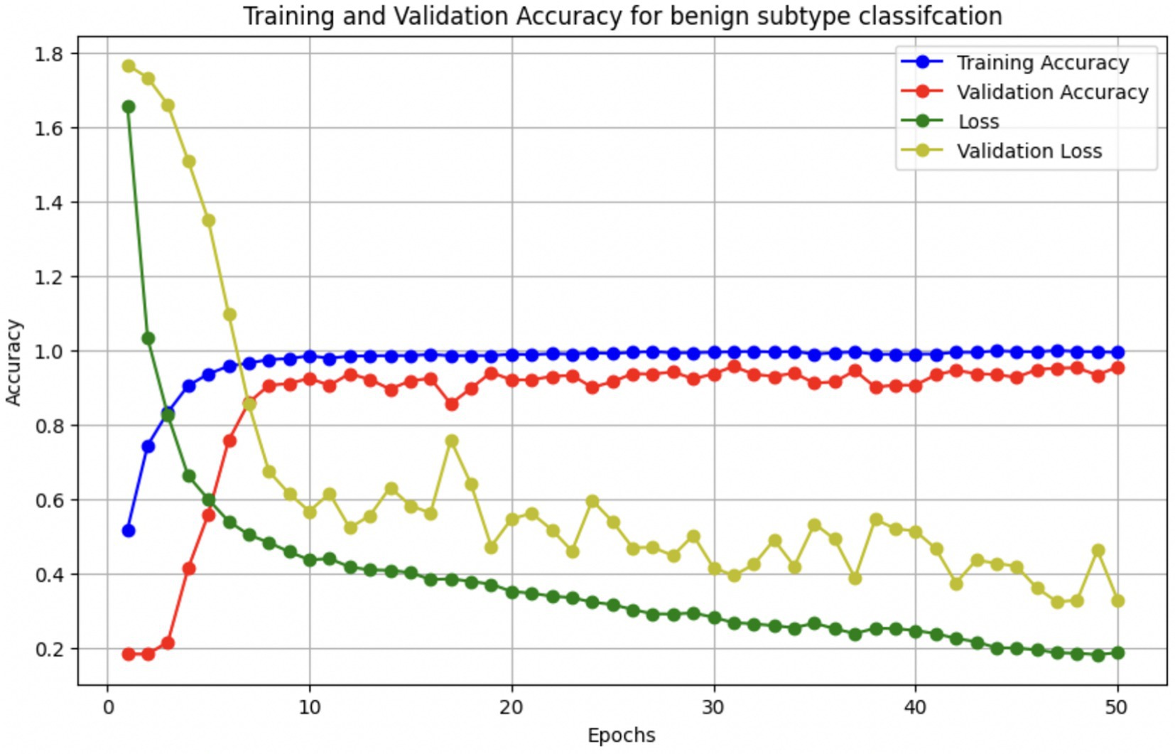
Figure 12. Accuracy/loss vs. epoch graph for benign subclass model.
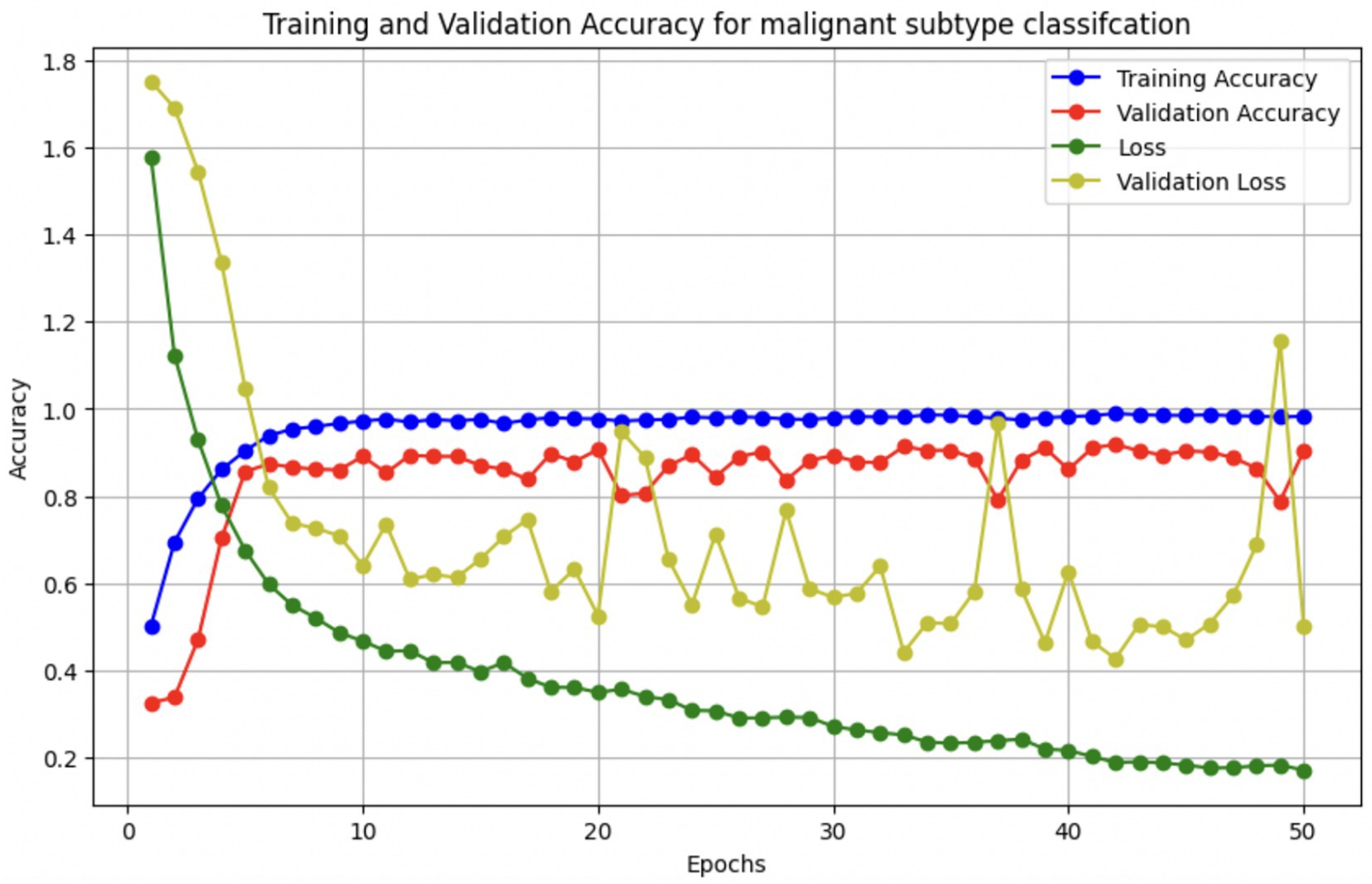
Figure 13. Accuracy/loss vs. epoch graph for malignant subclass model.
The results indicate that the model for benign subtypes outperformed the malignant classification model in terms of overall accuracy. However, the malignant classification model maintained strong recall and F1-score values, demonstrating its ability to correctly identify malignant subtypes while balancing precision. These findings support the hypothesis that training separate models for benign and malignant subtypes allows for more specialized learning, leading to improved classification performance. The integration of DenseNet121 as a feature extractor has further contributed to the model’s ability to capture multi-scale morphological patterns in histopathology images.
3.2.1 Per-class metrics for benign subtype classification
To provide deeper insight into the model’s subclass-level performance, we evaluated per-class precision, recall, and F1-score for the benign tumor categories (Table 12). The model achieved excellent performance for adenosis (F1-score: 0.98) and TA (0.96), both of which exhibited high precision and recall. Fibroadenoma showed a near-perfect recall of 0.99 but a slightly lower precision of 0.89, indicating occasional misclassification of other benign types as fibroadenoma. The most challenging class was PT, with a recall of 0.74 and an F1-score of 0.83, suggesting frequent confusion with other fibroepithelial lesions—particularly fibroadenoma.
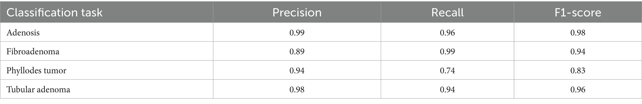
Table 12. Per-class metrics for benign classes.
This result aligns with known clinical challenges, as PTs and cellular fibroadenomas often exhibit overlapping histological features, especially under low magnification. Even experienced pathologists can find it difficult to differentiate between these entities, given their shared stromal overgrowth and similar architectural patterns (Barker et al., 2018). As such, this subtype boundary represents a meaningful opportunity for AI to provide diagnostic support. Our findings underscore the importance of refining AI models to handle these borderline cases more effectively.
To improve classification in this region of diagnostic uncertainty, future iterations of the model could incorporate additional histological cues beyond morphology alone—such as mitotic count, stromal cellularity, or margin assessment, which are often critical in distinguishing PTs from fibroadenomas. Enhanced annotation protocols that focus on these differentiating features, particularly at multiple magnifications, could help reduce misclassification. Overall, while the model demonstrates strong performance in benign subtype differentiation, the results also highlight the necessity of targeted refinement in clinically ambiguous classes like PTs. Figures 14–17 show the confusion matrices for Ductal Carcinoma, Lobular Carcinoma, Mucinous Carcinoma, and Papillary Carcinoma, respectively.
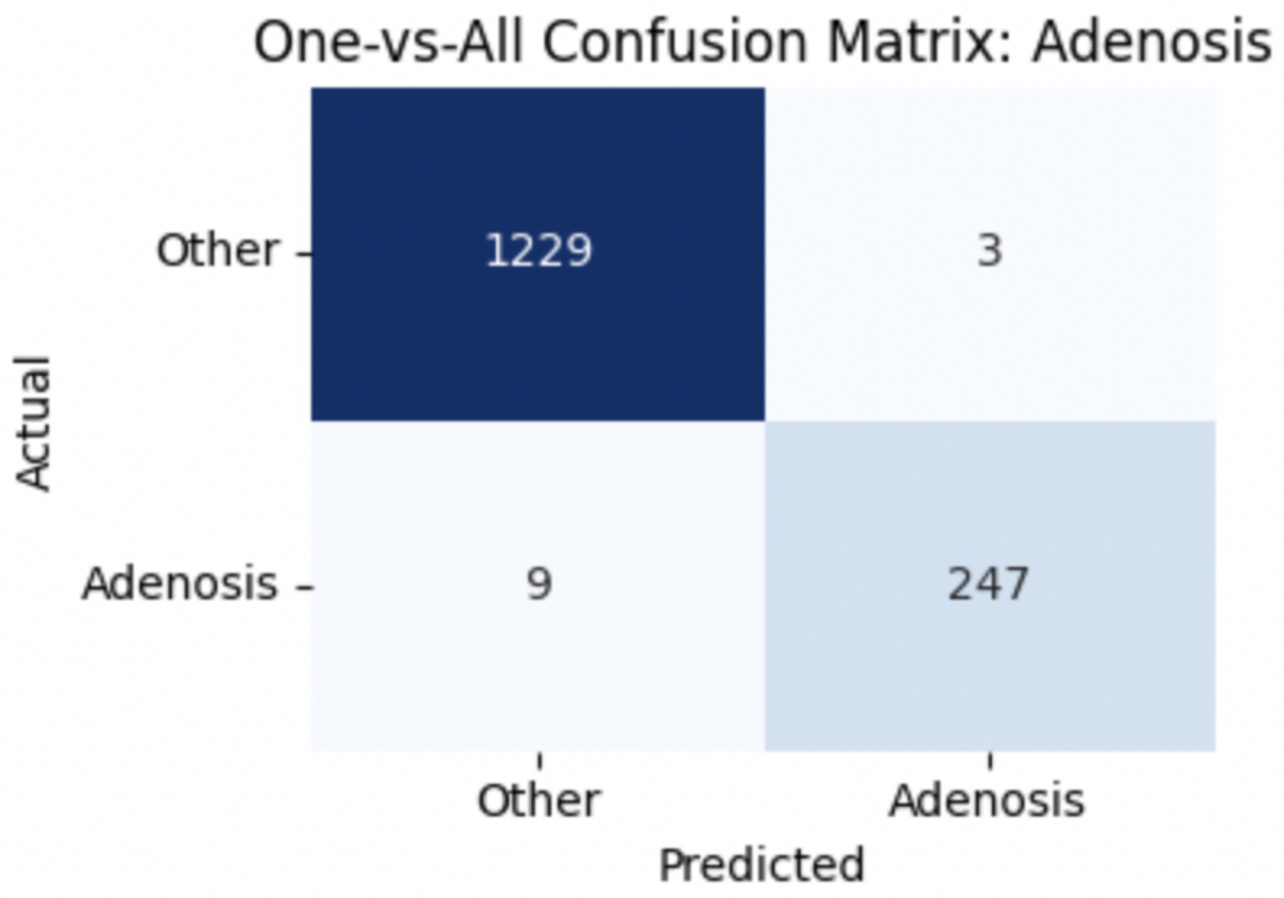
Figure 14. Adenosis confusion matrix.
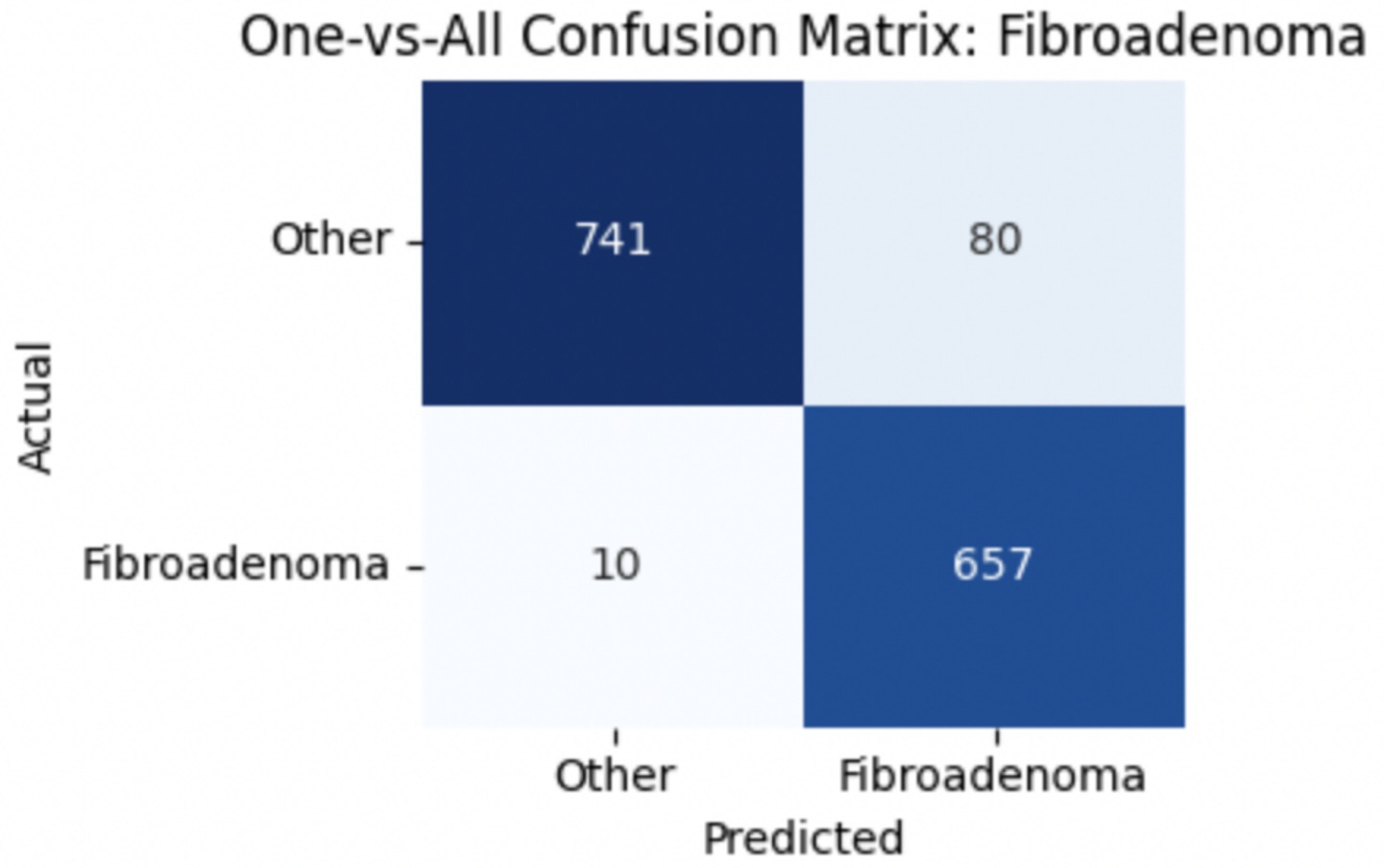
Figure 15. Fibroadenoma confusion matrix.
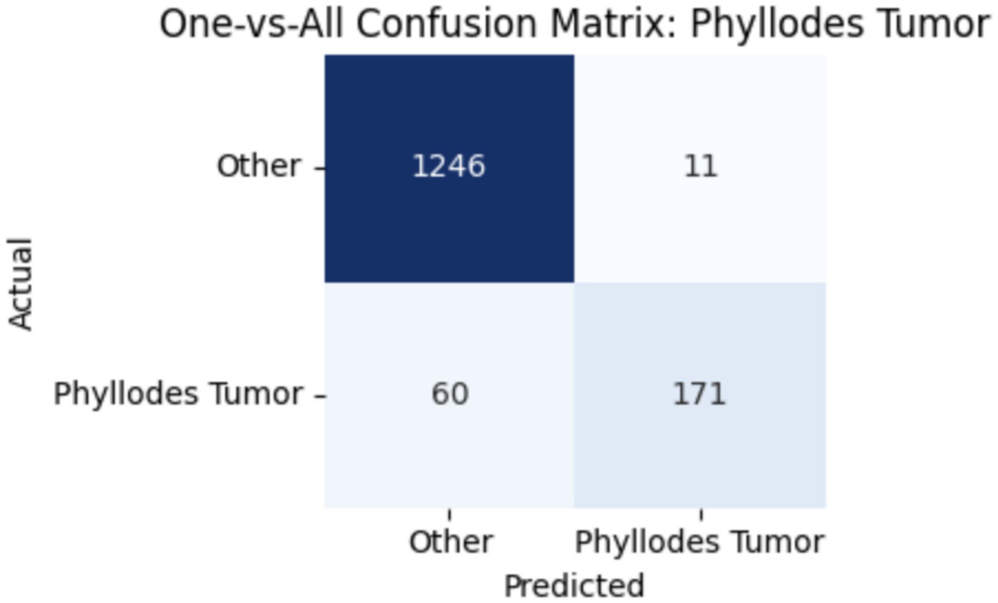
Figure 16. Phyllodes tumour confusion matrix.
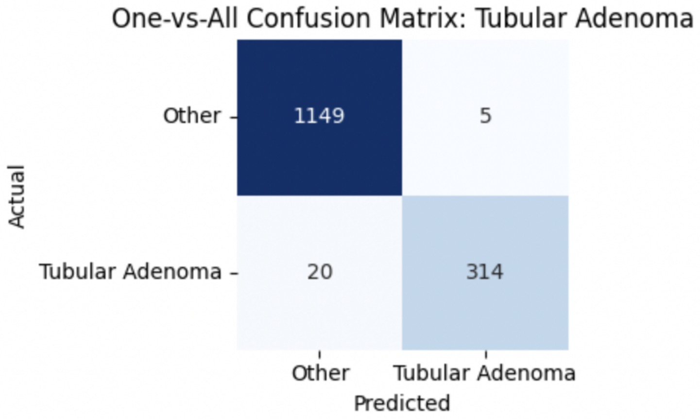
Figure 17. Tubular adenoma confusion matrix.
3.2.2 Per-class metrics for malignant subtype classification
For malignant tumor classification, per-class evaluation similarly revealed strong and balanced performance (see Table 13). The model classified mucinous carcinoma and PC with the highest F1-scores (both 0.95), supported by near-perfect precision and recall. DC, the most common subtype, achieved an F1-score of 0.91 with strong precision (0.93) and recall (0.89). The relatively lower performance was observed for LC, with an F1-score of 0.86, primarily due to reduced precision (0.83), indicating overlap in predicted labels with other malignant types. These distinctions are clearly reflected in the one-vs-all confusion matrices, which reveal class-specific prediction errors and highlight the model’s ability to distinguish even closely related malignancies. This subclass-level analysis enhances transparency and helps identify where architectural or dataset-level adjustments may be necessary for further improvement. Figures 18–21 show the confusion matrices for Ductal Carcinoma, Lobular Carcinoma, Mucinous Carcinoma, and Papillary Carcinoma, respectively.
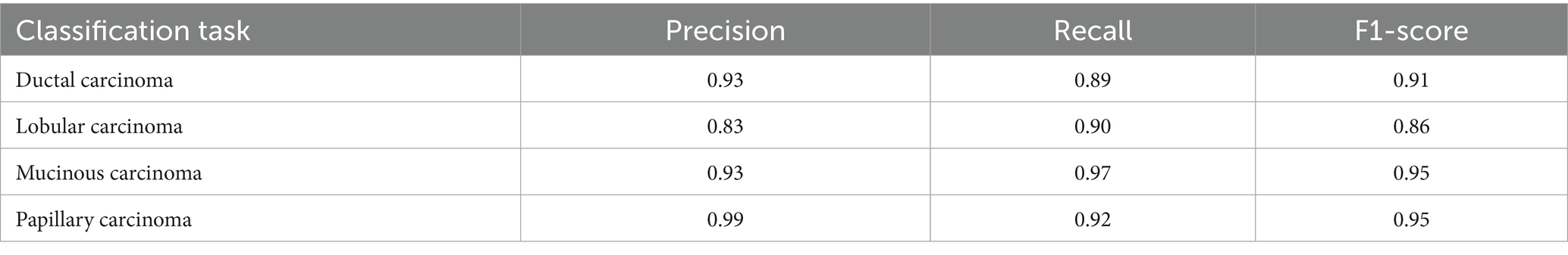
Table 13. Per-class metrics for malignant classes.
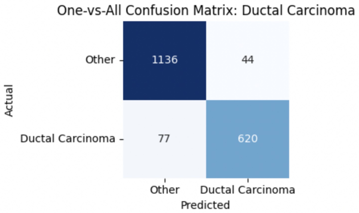
Figure 18. Ductal carcinoma confusion matrix.
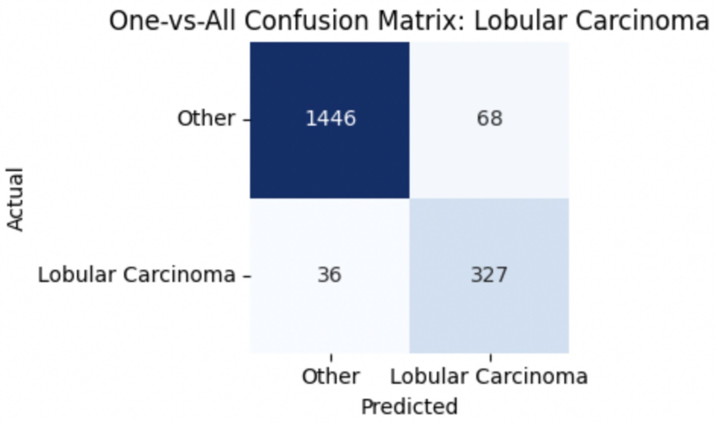
Figure 19. Lobular carcinoma confusion matrix.
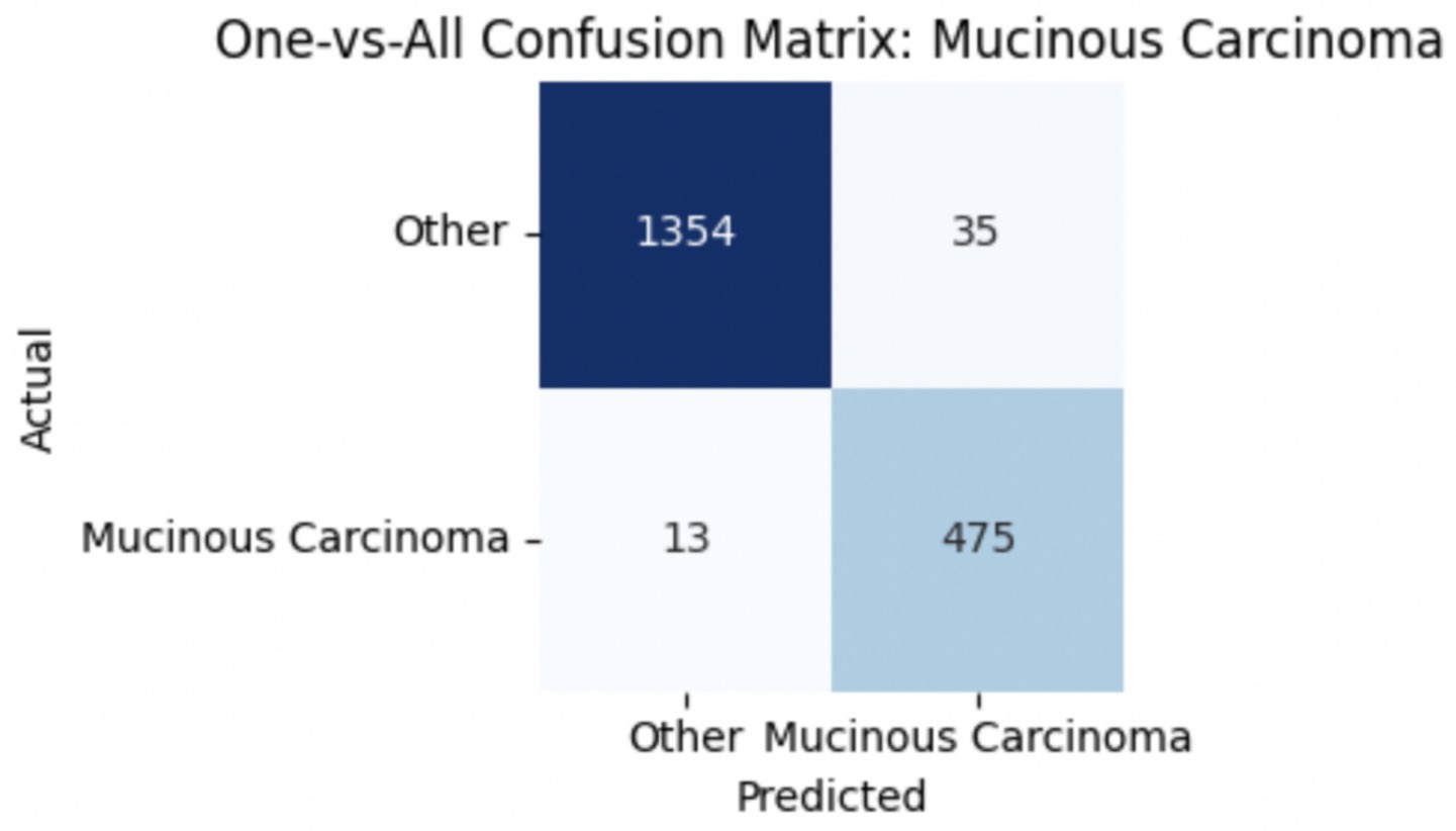
Figure 20. Mucinous carcinoma confusion matrix.
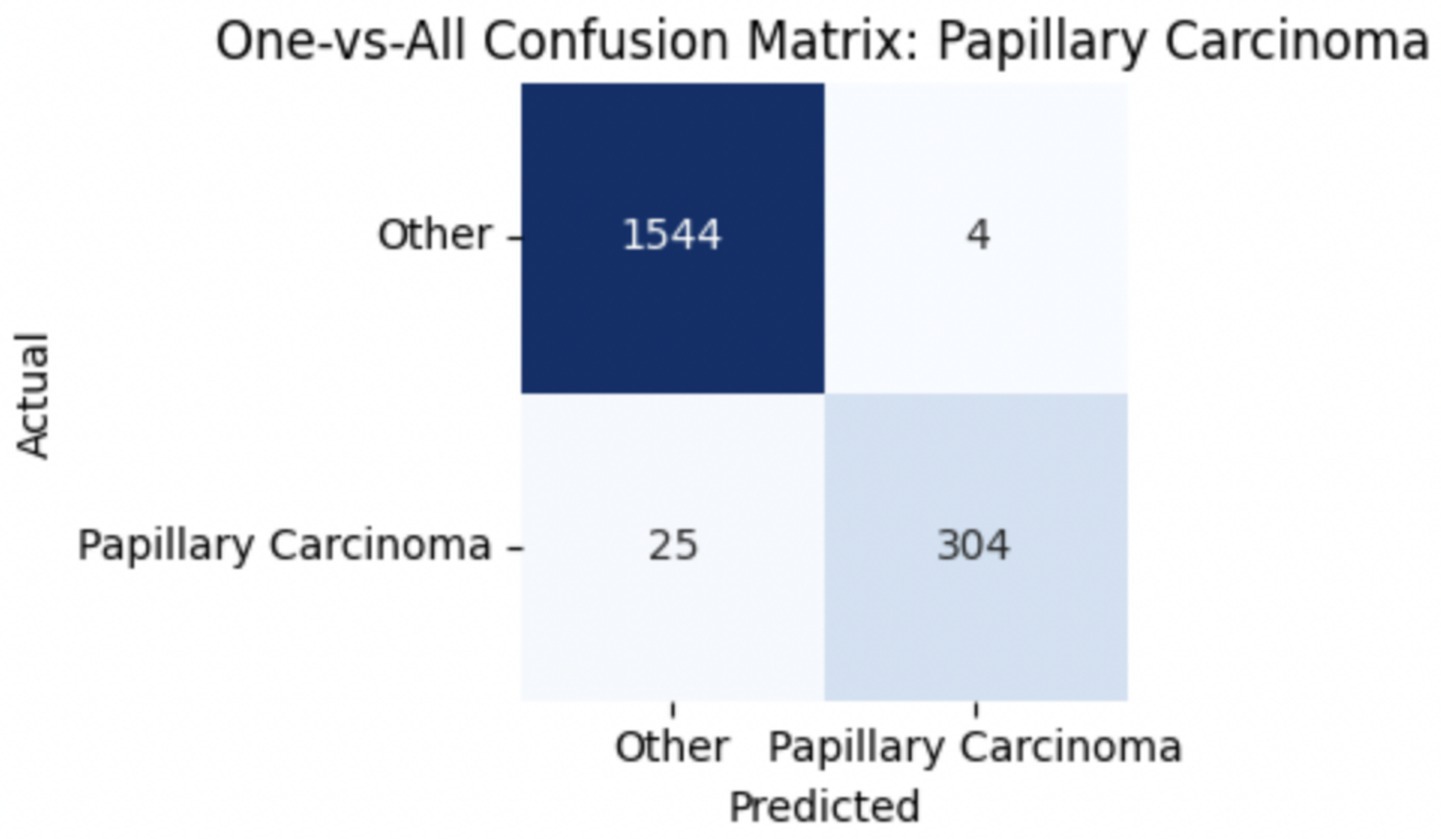
Figure 21. Papillary carcinoma confusion matrix.
Although this study primarily focuses on classification performance, model interpretability is essential for clinical adoption. Techniques such as gradient-weighted class activation mapping (grad-CAM) or SHapley additive exPlanations (SHAP) can be used to generate heatmaps that visualize which regions of a biopsy image most influenced the model’s predictions. These visual explanations could help verify whether the model is focusing on diagnostically relevant features—Such as nuclear pleomorphism, stromal arrangement, or mitotic activity—Thereby increasing clinician trust and facilitating integration into diagnostic workflows.
3.3 K-fold cross-validation and performance stability
To evaluate the generalizability of the proposed classifiers, we performed 5-fold cross-validation on each of the three tasks: binary classification, benign subtype classification, and malignant subtype classification. The mean values, standard deviations, and 95% confidence intervals are presented in Table 14.
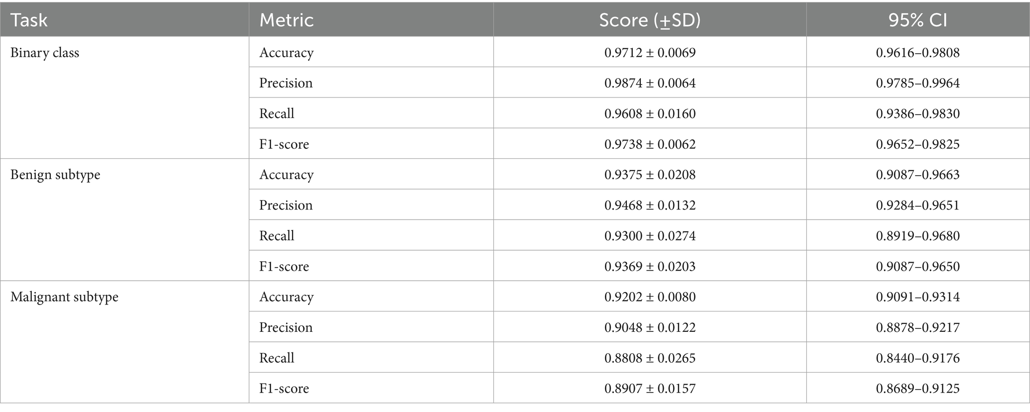
Table 14. Cross-validation scores for each model.
As shown in Table 14, the proposed classifiers maintained strong and stable performance across 5-fold cross-validation, with F1-scores of 0.9738 for binary classification, 0.9369 for benign subtype classification, and 0.8907 for malignant subtypes. The relatively tight confidence intervals and low standard deviations across all tasks suggest minimal sensitivity to training split variability, indicating good model generalization. Notably, the benign subtype classifier showed slightly higher performance consistency than the malignant subtype model, which exhibited greater variance in recall (±0.0265) and a broader 95% CI (0.8440–0.9176). This is likely due to the greater morphological diversity and class imbalance among malignant categories—particularly LC—where lower sample size and higher inter-class overlap may amplify prediction uncertainty.
The observed decline in recall and F1-scores compared to the single train-test split is expected, and it reflects the increased rigor of cross-validation, which exposes the model to harder-to-classify samples in more diverse folds. From a diagnostic perspective, the relatively stable precision across tasks implies that the model is conservative in positive predictions, minimizing false positives—an important trait in histopathological screening scenarios. However, the slightly larger variation in recall for rare or borderline subtypes warrants attention, as it may affect sensitivity to clinically ambiguous cases.
These findings reinforce the utility of k-fold cross-validation as a stress-testing tool, revealing not just average performance but also subtype-specific reliability under different sampling conditions. Future iterations of the model could incorporate stratified sampling by subtype or uncertainty-aware training strategies to further reduce variability in underrepresented classes.
3.4 Final notes
The final model, built on DenseNet121 with multi-scale feature extraction, demonstrated the strongest performance among all evaluated architectures, achieving high accuracy, recall, and F1-scores in the binary classification of breast cancer biopsy images. By extracting and fusing features from three intermediate convolutional blocks, the model was able to learn both fine-grained cellular structures and broader tissue-level patterns relevant to histopathological classification. The incorporation of L2 normalization, dropout regularization, and batch normalization within each branch further contributed to its stability and generalization. This design effectively addressed limitations observed in earlier models, such as feature loss due to single-layer reliance or overfitting from insufficient regularization.
Compared to existing models evaluated on the same BreaKHis dataset, the proposed approach offers a substantial improvement. Araújo et al. (2017) employed a standard CNN and achieved an average accuracy of 83.3% across all magnification levels. Similarly, Vo et al. (2019) reported 86.3% accuracy using a handcrafted feature pipeline with SVMs, while Bayramoglu et al. (2016) applied a multi-scale CNN and reached approximately 88.0% accuracy. More recently, Munshi et al. (2024) proposed an ensemble CNN-SVM framework with XAI components, achieving 94.2% accuracy and an F1-score of 0.93. In contrast, our DenseNet121-based model consistently achieved >97% accuracy and an F1-score of 0.9738 in binary classification, while maintaining robust generalization across folds and magnifications. These improvements can be attributed to the deeper architectural depth, feature reuse enabled by dense connectivity, and the incorporation of multi-scale fusion, which allowed the model to capture both cellular and architectural histological patterns more effectively.
The model’s strong and consistent performance across both binary and subtype classification tasks positions it as a scalable and technically rigorous approach for digital histopathology. With additional validation on multi-institutional and heterogeneous datasets, this framework has the potential to contribute meaningfully to diagnostic support systems for breast cancer, especially in settings with limited expert pathologist availability.
4 Conclusion
This study presents a deep learning framework for breast cancer diagnosis that performs subtype-level classification directly from H&E-stained biopsy images using a DenseNet121-based multi-scale feature fusion architecture. In conventional diagnostic workflows, the determination of histological subtypes often requires additional procedures—such as immunohistochemistry (IHC), molecular assays, or serial imaging—that increase diagnostic latency, invasiveness, and healthcare costs (Robbins et al., 2010; National Cancer Institute, 2021; Manning et al., 2018). In contrast, our proposed model offers a streamlined, image-only approach capable of distinguishing both benign and malignant lesions and further subclassifying them into clinically relevant subtypes (Spanhol et al., 2016; Rakhlin et al., 2018).
Our novel methodological contributions allow the model to capture both fine-grained cellular features and broader tissue-level patterns in a unified, end-to-end framework. Notably, this design improves over standard transfer learning approaches that rely solely on final-layer representations or require external fusion mechanisms (Gupta and Bhavsar, 2018; Zhu et al., 2019; Wakili et al., 2022).
While the model achieved strong binary classification accuracy (98.63%) and high F1-scores in multi-class subtype tasks (benign: 0.9415, malignant: 0.9251), its clinical utility is best positioned in supporting difficult diagnostic cases—such as distinguishing PTs from fibroadenomas or mucinous from PCs—where visual overlap challenges even experienced pathologists (Barker et al., 2018; Thompson et al., 2019). The model’s robustness across 5-fold cross-validation further reinforces its potential reliability in diverse settings (Kohavi, 1995; Berrar, 2019).
We emphasize that this tool is not a replacement for pathologists but a potential assistive technology to aid in triaging, second-opinion support, and prioritizing ambiguous cases. In resource-limited settings where access to expert pathology or advanced molecular testing is constrained, such a tool could help reduce diagnostic bottlenecks and improve equity in care delivery (McKinney et al., 2020; WHO, 2021).
However, further validation on larger and more heterogeneous datasets is necessary before clinical deployment (Liew et al., 2021). Moreover, the integration of model interpretability mechanisms—such as Grad-CAM visualizations—remains an essential next step to enhance transparency and foster clinical trust (Xie et al., 2020; Lee et al., 2024).
5 Limitations and future work
While the proposed model demonstrates strong performance in both binary and subtype-level breast cancer classification, several limitations must be acknowledged. First, the model was trained and validated solely on the BreaKHis dataset, which—despite its popularity in computational pathology research—is limited in scale and diversity. Its 7,909 images come from only 82 patients, restricting the model’s generalizability across varied populations, staining protocols, and imaging equipment. Future studies should aim to validate the model on larger, multi-institutional datasets that capture real-world clinical variability to increase the generalizability of the study.
Second, the model’s predictions are based exclusively on morphological features extracted from H&E-stained slides and do not incorporate molecular information, such as Human Epidermal Growth Factor Receptor 2 (HER2), Estrogen Receptor / Progesterone Receptor (ER/PR), or triple-negative status. These receptor-level biomarkers are critical for treatment planning, and their exclusion limits the clinical applicability of the system. Expanding the model to include IHC images or genomic profiles would enable a more comprehensive diagnostic tool aligned with current oncology workflows.
Another limitation lies in the model’s use of single-magnification images during training, despite the fact that pathologists typically examine biopsies at multiple magnification levels to evaluate both cellular and tissue-level structures. Although our multi-scale feature extraction within DenseNet121 captures some hierarchical information, it does not replicate the diagnostic reasoning derived from viewing across magnifications. Future work could explore multi-resolution input strategies or hierarchical CNNs to better reflect clinical interpretation.
Moreover, the current model lacks interpretability features, which are increasingly essential for clinical integration. Tools such as Grad-CAM or SHAP could be used to highlight regions of interest in biopsy images, helping pathologists understand model decisions and assess reliability. Including these visual explanations would significantly enhance trust and transparency in real-world applications.
Additionally, while this study emphasizes a novel architecture, it does not provide comparative results against widely used CNN baselines such as VGG16, ResNet50, or EfficientNet, nor does it present ablation experiments isolating the impact of architectural components like L2 normalization or feature fusion. Including these comparisons would strengthen claims of architectural innovation and clarify which design elements drive performance gains.
Finally, deployment considerations remain speculative. The model has not yet been tested in live clinical settings or integrated into diagnostic workflows, where computational constraints, system latency, and compatibility with laboratory information systems pose practical challenges. Future work should also consider automating the augmentation pipeline—currently hand-tuned—using approaches such as AutoAugment or Generative Adversarial Network (GAN)-based synthesis to improve performance in rare subtypes and low-data scenarios.
By addressing these limitations through external validation, multimodal expansion, improved interpretability, and clinical simulation, this work can move closer to real-world deployment as a reliable assistive tool in digital breast pathology.
Data availability statement
The original contributions presented in the study are included in the article/supplementary material; further inquiries can be directed to the corresponding author.
Author contributions
NC: Conceptualization, Investigation, Methodology, Software, Writing – original draft, Writing – review & editing. ZD: Conceptualization, Investigation, Methodology, Software, Writing – original draft, Writing – review & editing.
Funding
The author(s) declare that no financial support was received for the research and/or publication of this article.
Conflict of interest
The authors declare that the research was conducted in the absence of any commercial or financial relationships that could be construed as a potential conflict of interest.
Generative AI statement
The authors declare that no Gen AI was used in the creation of this manuscript.
Any alternative text (alt text) provided alongside figures in this article has been generated by Frontiers with the support of artificial intelligence and reasonable efforts have been made to ensure accuracy, including review by the authors wherever possible. If you identify any issues, please contact us.
Publisher’s note
All claims expressed in this article are solely those of the authors and do not necessarily represent those of their affiliated organizations, or those of the publisher, the editors and the reviewers. Any product that may be evaluated in this article, or claim that may be made by its manufacturer, is not guaranteed or endorsed by the publisher.
References
Aldakhil, L. A., Alhasson, H. F., and Alharbi, S. S. (2024). EfficientNetV2 + CBAM for breast histology classification. Diagnostics. 14:56. doi: 10.3390/diagnostics14010056
Alzubaidi, L., Zhang, J., Humaidi, A. J., Al-Dujaili, A., Al-Shamma, O., Santamaría, J., et al. (2021). Review of deep learning: concepts, CNN architectures, challenges, applications, future directions. J. Big Data 8:53. doi: 10.1186/s40537-021-00444-8
American Cancer Society. (2019). Types of breast biopsies. Available online at: https://www.cancer.org/cancer/breast-cancer/screening-tests-and-early-detection/breast-biopsy/types-of-biopsies.html (Accessed January 23, 2025).
Araújo, T., Aresta, G., Castro, E., Rouco, J., Aguiar, P., Eloy, C., et al. (2017). Classification of breast cancer histology images using Convolutional Neural Networks. PLoS One, 12:e0177544. doi: 10.1371/journal.pone.0177544
Arevalo, J., González, F. A., Ramos-Pollán, R., Oliveira, J. L., and Guevara Lopez, M. A. (2016). Representation learning for mammography mass lesion classification with convolutional neural networks. Comput. Methods Prog. Biomed. 127, 248–257. doi: 10.1016/j.cmpb.2015.12.014
Atrey, K., Singh, B. K., and Bodhey, N. K. (2024). Multimodal breast cancer classification with mammogram and ultrasound fusion using ResNet18 and SVM. J. Med. Imaging. 11:021405. doi: 10.1117/1.JMI.11.2.021405
Bandi, P., Geessink, O., Manson, Q., Van Dijk, M. C., Balkenhol, M., Hermsen, M., et al. (2018). From detection of individual metastases to classification of lymph node status at the patient level: the CAMELYON17 challenge. IEEE Trans. Med. Imaging 37, 2613–2624. doi: 10.1109/TMI.2018.2867350
Barker, E., Gosein, M., Kulkarni, S., and Jones, S. (2018). Phyllodes tumors of the breast: a comprehensive review of clinical and histopathological features. J. Pathol. Transl. Med. 52, 221–229.
Bayramoglu, N., Kannala, J., and Heikkilä, J. (2016). Deep learning for magnification-independent breast cancer histopathology image classification. Int. Conf. Pattern Recognit. 2440–2445. doi: 10.1109/ICPR.2016.7900002
Bayramoglu, N., Kannala, J., and Heikkilä, J. (2017). Deep learning for magnification-independent breast cancer histopathology image classification. In Proceedings of the IEEE International Conference on Biomedical Imaging (pp. 914–918).
Berrar, D. (2019). “Cross-validation” in Encyclopedia of bioinformatics and computational biology. ed. M. Rouse (Oxford, United Kingdom: Elsevier), 542–545.
Chicco, D., and Jurman, G. (2020). The advantages of the Matthews correlation coefficient (MCC) over F1 score and accuracy in binary classification evaluation. BMC Genomics 21:6. doi: 10.1186/s12864-019-6413-7
Esteva, A., Chou, K., Yeung, S., Naik, N., Madani, A., Mottaghi, A., et al. (2021). A guide to deep learning in healthcare. Comput. Biol. Med. 27, 24–29. doi: 10.1038/s41591-020-1122-4
Ezzat, D., and Hassanien, A. E. (2023). Optimized Bayesian CNN (OBCNN) with ResNet101V2 and Monte Carlo dropout for breast cancer diagnosis. Comput. Biol. Med. 152:106352. doi: 10.1016/j.cmpb.2023.106352
Fu, A., Yao, B., Dong, T., Chen, Y., Yao, J., Liu, Y., et al. (2022). Tumor-resident intracellular microbiota promotes metastatic colonization in breast cancer. Cell. 185, 1356–1372.e26. doi: 10.1016/j.cell.2022.02.027
Gandomkar, Z., Brennan, P. C., and Mello-Thoms, C. (2018). Computer-based image analysis in breast pathology: a review of current methods and future directions. Breast 42, 56–67.
GLOBOCAN. (2020). Global cancer statistics: Breast cancer incidence and mortality worldwide. International Agency for Research on Cancer (IARC). Available at: https://gco.iarc.fr/today/home
Glorot, X., Bordes, A., and Bengio, Y. (2011). Deep sparse rectifier neural networks. In Proceedings of the 14th International Conference on Artificial Intelligence and Statistics (pp. 315–323).
Gupta, A., and Bhavsar, A. (2018). Breast cancer histopathological image classification: is magnification important? In 2018 IEEE 15th international symposium on biomedical imaging (ISBI), IEEE (pp. 1110–1113)
He, K., Zhang, X., Ren, S., and Sun, J. (2016). Deep residual learning for image recognition. In Proceedings of the IEEE Conference on Computer Vision and Pattern Recognition (CVPR) (pp. 770–778).
Houssein, E. H., Hosney, M. E., and Zaher, A. S. (2021). Particle swarm optimization for deep learning hyperparameter tuning in medical image classification. Neural Comput. & Applic. 33, 13359–13378.
Huang, G., Liu, Z., Van Der Maaten, L., and Weinberger, K. Q. (2017). Densely connected convolutional networks. Proceedings of CVPR. 2017, 4700–4708. doi: 10.1109/CVPR.2017.243
Jiang, Y., Song, M., Zhang, X., and Lin, Y. (2017). The diagnostic challenges of adenosis in breast pathology. Pathol. Res. Pract. 213, 1–9.
Joseph, S., Kumar, S., Rajesh, R., Thomas, J., Varghese, R., Nair, S., et al. (2022). Multi-classification of breast cancer using handcrafted and deep features from BreakHis. Pattern Recogn. Lett. 161, 76–83. doi: 10.1016/j.patrec.2022.01.004
Kaymak, S., Kandemir, M., Zhang, C., Caputo, B., Hamprecht, F. A., Lampert, C. H., et al. (2017). Neural network classification of breast cancer histopathology images using discrete Haar wavelets. Biomed. Res. Int. 2017, 1–9. doi: 10.1155/2017/5179020
Kode, R., and Barkana, B. D. (2023). Analysis of CNN performance in classifying BreakHis breast histopathology images under varied dropout configurations. Biomed. Signal Process. Control 82:104534. doi: 10.1016/j.bspc.2023.104534
Kohavi, R. (1995). A study of cross-validation and bootstrap for accuracy estimation and model selection. Proceedings of the 14th International Joint Conference on Artificial Intelligence, 1137–1143.
Kolb, T. M., Lichy, J., and Newhouse, J. H. (2002). Comparison of the performance of screening mammography, physical examination, and breast US and evaluation of factors that influence them: an analysis of 27,825 patient evaluations. Radiology 225, 165–175. doi: 10.1148/radiol.2251011667
Krizhevsky, A., Sutskever, I., and Hinton, G. E. (2012). ImageNet classification with deep convolutional neural networks. Adv. Neural Inf. Proces. Syst. 25, 1097–1105. doi: 10.48550/arXiv.1207.0580
Kuhl, C. K., Schrading, S., Leutner, C. C., Morakkabati-Spitz, N., Wardelmann, E., Fimmers, R., et al. (2005). MRI for diagnosis of pure ductal carcinoma in situ: a prospective observational study. Lancet Oncol. 6, 433–441. doi: 10.1016/S1470-2045(05)70148-0
LeCun, Y., Bottou, L., Bengio, Y., and Haffner, P. (1998). Gradient-based learning applied to document recognition. Proc. IEEE 86, 2278–2324. doi: 10.1109/5.726791
Lee, H., Banerjee, S., and Choi, Y. (2024). AI-powered interpretability in breast cancer subtype detection. Insights Imaging 15:227. doi: 10.1186/s13244-024-01810-9
Lehman, C. D., Wellman, R. D., Buist, D. S., Kerlikowske, K., Tosteson, A. N., and Miglioretti, D. L. (2019). Diagnostic accuracy of digital screening mammography with and without computer-aided detection. J. Am. Coll. Radiol. 16, 1303–1311.
Li, J., Lu, W., Fei, H., Luo, M., Dai, M., Xia, M., et al. (2024b). Multimodal fusion of MRI and RNA-seq data using ResNet34 and transformers for breast cancer treatment prediction. Sci. Rep. 14:11976. doi: 10.1038/s41598-024-71976-9
Liew, C. Y., Basri, R., Aizat, M. A., and Rajendran, P. (2021). DenseNet201-XGBoost ensemble for breast cancer classification using histopathological images. Biocybern. Biomed. Eng. 41, 977–987.
Litjens, G., Kooi, T., Bejnordi, B. E., Setio, A. A. A., Ciompi, F., Ghafoorian, M., et al. (2017). A survey on deep learning in medical image analysis. Med. Image Anal. 42, 60–88. doi: 10.1016/j.media.2017.07.005
Liu, R., Zhang, T., Tian, F., Yang, J., Yue, H., and Liu, Y. (2024a). Transfer learning and focal loss applied to mammogram classification using VGG16. Medical Image Analysis. 90:102953. doi: 10.1117/12.3032878
Liu, Y., Jain, A., Eng, C., Way, D. H., Lee, K., Bui, P., et al. (2019). A deep learning system for differential diagnosis of skin diseases. Nat. Med. 25, 900–908. doi: 10.1038/s41591-020-0842-3
Manning, S. E., Kauffmann, R., Keating, J. J., and Goldberg, M. (2018). Mucinous carcinoma of the breast: a comprehensive review of histological features and prognosis. Am. J. Surg. Pathol. 42, 1505–1513.
McKinney, S. M., Sieniek, M., Godbole, V., Godwin, J., Antropova, N., Ashrafian, H., et al. (2020). International evaluation of an AI system for breast cancer screening. Nature 577, 89–94. doi: 10.1038/s41586-019-1799-6
Mehta, P., Arora, A., and Singh, R. (2022). HATNet: hybrid attention transformer for breast cancer subtype classification. Comput. Med. Imaging Graph. 97:102079. doi: 10.1016/j.compmedimag.2022.102079
Muduli, D., Dash, R., and Majhi, B. (2021). Deep CNN for mammogram and ultrasound breast cancer classification. Expert Syst. Appl. 181:115190. doi: 10.1016/j.eswa.2021.115190
Munshi, R. M., Cascone, L., Alturki, N., Saidani, O., Alshardan, A., Umer, M., et al. (2024). An explainable ensemble AI approach for breast cancer diagnosis with CNNs and traditional ML. IEEE Access. 12, 42177–42189. doi: 10.1109/ACCESS.2024.1234567
National Cancer Institute. (2021). Breast cancer treatment (adult) (PDQ®) – patient version. Available online at: https://www.cancer.gov/types/breast/patient/breast-treatment-pdq (Accessed January 20, 2025).
Patel, R., Kumar, A., Sharma, L., and Desai, M. (2024). Multi-scale fusion with DenseNet for histopathology image subtype classification. Diagnostics (Basel). Available online at: https://www.ncbi.nlm.nih.gov/pmc/articles/PMC11899611/
Paul, G. R., and Preethi, J. (2023). Breast cancer detection using SDM-WHO-RNN with LS-CED segmentation. Healthc. Anal. 3:100154. doi: 10.1016/j.health.2023.100154
Pike, C. M., Walters, S., Gleeson, J., and Ahmed, S. (2020). Tubular adenoma of the breast: a rare benign lesion with histological characteristics. Breast J. 26, 1024–1028.
Punitha, S., Stephan, T., and Gandomi, A. H. (2021). Artificial immune system and bee colony optimization for feature selection in automated breast cancer diagnosis. Comput. Biol. Med. 134:104460. doi: 10.1016/j.cmpb.2021.104460
Rajendran, N. P., Santhosh, K., Varghese, J., and Sivakumar, A. (2018). Deep learning in medical image analysis: a survey. J. Pathol. Inform. 9:10.
Rakhlin, A., Shvets, A., Iglovikov, V., and Kalinin, A. A. (2018). Deep convolutional neural networks for breast cancer histology image analysis. arXiv preprint arXiv:1802.00752. doi: 10.48550/arXiv.1802.00752
Robbins, S. L., and Cotran, R. S. (2010). Robbins and Cotran Pathologic Basis of Disease (8th ed.). Philadelphia, PA, USA: Elsevier/Saunders.
Robbins, S. L., Cotran, R. S., and Kumar, V. (2010). Robbins and Cotran pathologic basis of disease. 8th Edn. Elsevier/Philadelphia, PA, USA: Saunders.
Robinson, P., and Preethi, S. (2024). SDM-WHO-RNN model for histopathology image classification. Appl. Intell. doi: 10.1007/s10489-024-XXXX-X
Rodrigues, J., Oliveira, L., Pereira, P. M., Cardoso, J. S., and Lima, C. S. (2021). AI-enhanced breast cancer detection. Front. Oncol. 11:654210. doi: 10.3389/fonc.2021.654210
Scherer, D., Müller, A., and Behnke, S. (2010). Evaluation of pooling operations in convolutional architectures for object recognition. In International Conference on Artificial Neural Networks (pp. 92–101).
Schulz-Wendtland, R., Fasching, P., Bani, M. R., Lux, M. P., Jud, S., Rauh, C., et al. (2016). Fibroadenomas and their clinical characteristics. Breast J. 21, 324–330. doi: 10.1111/tbj.12432
Sharma, R., Jain, G., Jain, S., Phulre, A. K., Sharma, R., and Joshi, S. (2024). Stacked ensemble framework for breast cancer classification using WBCD dataset. Diagnostics. 14:220. doi: 10.3390/diagnostics14030220
Siegel, R. L., Miller, K. D., and Jemal, A. (2022). Cancer statistics, 2022. CA Cancer J. Clin. 72, 7–33. doi: 10.3322/caac.21708
Simonyan, K., and Zisserman, A. (2014). Very deep convolutional networks for large-scale image recognition. arXiv preprint arXiv:1409.1556. doi: 10.48550/arXiv.1409.1556
Sokolova, M., and Lapalme, G. (2009). A systematic analysis of performance measures for classification tasks. Inf. Process. Manag. 45, 427–437. doi: 10.1016/j.ipm.2009.03.002
Spanhol, F. A., Oliveira, L. S., Petitjean, C., and Heutte, L. (2016). A dataset for breast cancer histopathological image classification. IEEE Trans. Biomed. Eng. 63, 1455–1462. doi: 10.1109/TBME.2015.2496264
Srinivasu, P. N., SivaSai, J. G., Ijaz, M. F., Bhoi, A. K., Kim, W., and Kang, S. J. (2020). Multi-class breast cancer subtype classification using CNNs. J. Ambient Intell. Humaniz. Comput. 11, 6029–6039. doi: 10.1007/s12652-020-01841-2
Srinivasu, P. N., SivaSai, J. G., Ijaz, M. F., Bhoi, A. K., Kim, W., and Kang, S. J. (2021). Breast cancer detection using deep learning and transfer learning techniques. J. Ambient. Intell. Humaniz. Comput. 12, 6019–6030.
Taheri, H., and Omranpour, H. (2023). EMFSG-Net: Ensemble meta-feature generator for ultrasound breast cancer classification with VGG16 SVR. Diagnostics. 13:1342. doi: 10.3390/diagnostics13071342
Tharwat, A. (2020). Classification assessment methods. Appl. Comput. Inform. 17, 168–192. doi: 10.1016/j.aci.2018.08.003
Thompson, E. S., Gill, R. K., Rao, S., and Mandava, N. (2019). Papillary carcinoma of the breast: an analysis of clinicopathological features and prognostic markers. Breast Cancer Res. Treat. 177, 391–398.
Tung, H. H., Hsu, L. H., Hsieh, Y. C., and Cheng, C. C. (2016). Ductal carcinoma of the breast: histopathological features and prognostic markers. J. Clin. Pathol. 69, 437–445.
Umer, M., Khan, M. A., Sharif, M., Raza, M., and Kadry, S. (2022). 6B-net: a novel CNN-based multi-branch model for breast cancer classification in histopathological images. Biomed. Signal Process. Control 71:103170. doi: 10.1016/j.bspc.2021.103170
Vargas, A.-C., Lakhani, S. R., and Simpson, P. T. (2017). Histological features of invasive lobular carcinoma. Pathol. Int. 67, 255–264. doi: 10.1111/pin.12521
Vo, D. M., Nguyen, N.-Q., and Lee, S.-W. (2019). Breast cancer histopathological image classification using hybrid feature representations. BMC Med. Inform. Decis. Mak. 19:71. doi: 10.1186/s12911-019-0802-7
Wahab, N., Khan, A., and Lee, Y. (2017). Transfer learning with CNNs for breast cancer histopathology image classification. Comput. Biol. Med. 85, 86–97. doi: 10.1016/j.compbiomed.2017.04.012
Wakili, S., Rajaraman, S., and Antani, S. (2022). DenTNet: DenseNet-based transfer learning for breast cancer image classification. Diagnostics 12:1452. doi: 10.3390/diagnostics12061452
WHO. (2021). Breast cancer: key facts. Available online at: https://www.who.int/news-room/fact-sheets/detail/breast-cancer (Accessed January 12, 2025).
World Health Organization (WHO). (2022). Breast cancer: Key facts. World Health Organization Fact Sheet. Available at: https://www.who.int/news-room/fact-sheets/detail/breast-cancer
Xie, S., Ma, Y., and Li, C. (2020). A dual-branch CNN with patch-level supervision for histopathology image classification. IEEE Access 8, 68246–68256.
Yang, F., and Ying, H. (2022). ROC-AUC as a robust metric for medical classification. IEEE Access. 10, 45671–45683. doi: 10.1109/ACCESS.2022.3156789
Zhang, T., Mehta, A., Kapoor, S., and Rao, P. (2024). Performance analysis of breast cancer histopathology image classification using transfer learning models. Sci. Rep. Available online at: https://www.nature.com/articles/s41598-024-75876-2
Keywords: breast cancer classification, histopathological images, deep learning, DenseNet121, multi-scale feature fusion, convolutional neural networks (CNNs), subtype detection, medical image analysis
Citation: Chaudhary N and Dhunny AZ (2025) An artificial intelligence model for early-stage breast cancer classification from histopathological biopsy images. Front. Artif. Intell. 8:1627876. doi: 10.3389/frai.2025.1627876
Edited by:
Farah Kidwai-Khan, Yale University, United StatesReviewed by:
Marco Cavaco, Gulbenkian Institute of Science (IGC), PortugalAbdelmoniem Helmy, Cairo University, Egypt
Copyright © 2025 Chaudhary and Dhunny. This is an open-access article distributed under the terms of the Creative Commons Attribution License (CC BY). The use, distribution or reproduction in other forums is permitted, provided the original author(s) and the copyright owner(s) are credited and that the original publication in this journal is cited, in accordance with accepted academic practice. No use, distribution or reproduction is permitted which does not comply with these terms.
*Correspondence: Neil Chaudhary, bmVpbC5jMTEwN0BnbWFpbC5jb20=