A Low-Complexity Reconfigurable Multi-Antenna Technique for Non-Terrestrial Networks

1 Introduction

The next generation non-terrestrial networks (NTNs) are expected to be largely based on High or Low Altitude Platforms (HAPs/LAPs) and Unmanned Aerial Vehicles (UAVs). The true wireless connectivity in beyond 5G NTNs and the corresponding requirements for increased spectral and energy efficiency, higher data rates, lower latency, and support of massive Internet of Things (IoT) devices, call for enhanced signal processing techniques in all transceivers and network control systems.

The research in wireless systems and techniques for NTNs spans many domains, from massive-MIMO systems Chandhar et al. (2018), Geraci et al. (2018), mm-wave technologies and channel issues Zhang et al. (2019), Michailidis et al. (2020a), UAV selection Bithas et al. (2020), beam management and tracking Rinaldi et al. (2021), Zhao et al. (2018), to resource management in several multiple access schemes and especially non-orthogonal multiple access (NOMA) Ramírez and Mosquera (2020), Yan et al. (2019), and Artificial Intelligence (AI) techniques for system optimization Jiang and Zhu (2020), Ding et al. (2020), Michailidis et al. (2020b).

Multi-antenna systems have been proposed and utilized the last 20 yr to achieve increased throughput and reliability through antenna diversity, spatial multiplexing, and beamforming. Indeed, diversity systems have been widely adopted in various wireless communication scenarios for improving the spectral and power efficiency. Various methods for achieving diversity exist including: space, angle, polarization, frequency, multipath, and time. In this context, antenna or beam selection Molisch et al. (2005), Karamalis et al. (2006), Bai et al. (2011), has been proposed in wireless systems in order to exploit the advantages of diversity, while keeping the hardware complexity to a minimum. Under the same principle, pattern reconfigurable antenna arrays have been proposed for further improving the performance of wireless communication systems.

Generally, a radio system is able to generate a variety of radiation patterns, if it is equipped with multi-element antenna arrays, able to provide some beamforming capabilities. However, a multiple-input multiple-output (MIMO) configuration, that includes a multitude of RF chains, introduces hardware complexity, increases cost, requires careful management of the power efficiency and imposes increased array dimensions. Therefore, the direct application of the various multi-antenna techniques to an aerial communication system is not always feasible due to the constraints induced by the aerial platforms, e.g., the antenna weight/size, the requirement for extensive RF cabling, the low power and signal processing capabilities. Steerable and controllable intelligent antenna technologies could provide the means to cope with these problems and thus they are considered as ideal candidates to be adopted in the aerial communication platforms that will be used in the 5G and beyond communication networks.

An alternative MIMO implementation with low complexity is provided through the Electronically Steerable Parasitic Array Radiators (ESPARs) Kalis et al. (2008), Kalis et al. (2014). The ESPARs are reconfigurable antennas of reduced size and complexity, that are able to provide beamforming capabilities to the system through pattern adaptation Sun et al. (2004), Ohira and Gyoda (2000), Vasileiou et al. (2013). The ESPARs are able to produce multiple beam patterns using only one active element and consequently one RF chain. Pattern reconfigurability is achieved by electronically adjusting the loads of the parasitic elements that are distributed closely to the active. More specifically, the close proximity among elements causes significant mutual coupling effects and induces strong current flows on the parasitics, thus reconfiguring the radiation pattern. Consequently, the reduced complexity, cost and improved performance of the reconfigurable antennas has recently attracted the interest of the research community in the area of UAV-enabled communications, e.g., Choi and Lee (2020); Kim et al. (2020); Wolfe et al. (2018).

In this paper, a joint Tx-Rx beamforming with beam selection and combining technique is proposed for improving the performance of an aerial communication system supported by electronically steerable antenna arrays. The main idea of the proposed scheme is to select, using SNR maximization, a pair of beam patterns between each RF chain of the ground station and the aerial platform, and combine the received SNRs under the maximal ratio principle. Initially, an analytical stochastic framework has been developed that is based on a Markov chain model, which is used to investigate the statistics of the received SNR. Then, an implementation of the novel beamforming scheme is presented, with the introduction of an ESPAR antenna suitable for the UAV use case. In addition, a realistic simulator has been developed based on the Quadriga channel model Jaeckel et al. (2014) and the 3GPP-NR channel model TR38.901 (2018), by the aid of which the performance of the proposed scheme has been evaluated in conjunction with the extracted analytical results.

The rest of the paper is organized as follows. In Section 2, the system and channel models under investigation are presented, while in Section 3, the stochastic analytical framework is provided. Moreover, a low-complexity implementation of an antenna pattern dynamic reconfiguration scheme using ESPARs is presented and evaluated in Section 4. Finally, in Section 5, the concluding remarks are provided.

Notation: In the following analysis, bold variables denote matrices and vectors; ${\left[\mathbf{x}\right]}_m$ denotes the m-th element of the vector, while if the argument is a matrix, ${\left[\mathbf{A}\right]}_m$ denotes the m-th column of matrix $\mathbf{A}$, ${\left[{\mathbf{A}}^T\right]}_m^T$ denotes the m-th row of matrix, and ${\left[\mathbf{A}\right]}_{m,n}$ the element of the m-th row, n-th column. Finally, $\parallel .{\parallel }_F$ denotes the Frobenius norm.

2 System and Channel Models

In this section the reverse link of a UAV-enabled communication system is considered, in which the ground station (GS) supports two radio frequency (RF) chains, while the UAV is equipped with one RF chain. Moreover, all the signal processing operations are performed at the GS, while if necessary, the channel reciprocity is exploited. Such an approach agrees with the recent 5G standards related to the New Radio (NR), while it reduces the signal processing requirements, and thus the power consumption, on the UAVs. The latter is a critical parameter for extending the operational capabilities of the UAVs. Moreover, all RF chains are equipped with reconfigurable antennas, which are able to provide L different radiation patterns. Therefore, for each pair of Tx-Rx RF chains, $M=L^2$ different beam pairs can be obtained. Despite the fact that the proposed scheme focuses on the reverse link, it can also be applied in the forward link. Moreover, perfect channel state information (CSI) is assumed to be available at the receiver. Next, the system and channel models are analytically described.

2.1 Mode of Operation

One important goal of the proposed scheme is to reduce the requirements for CSI processing as well as to reduce the switching operations among the beam pairs, without considerably affecting the performance gain that is achieved due to the use of multiple antennas and beamforming. To this aim, the system combines a specific beam-pair from one of the two GS RF chains, with the beam-pair offering the highest received SNR from the other RF-chain. The mode of operation of the proposed scheme is depicted in Figure 1 and will be described next. Let ${\gamma }_i\left(n\right)$ denote the received SNR from the (selected) beam-pair of GS RF chain i at time instance n. Moreover, let ${\gamma }_{\overline{i}}^{\text{max}}\left(n\right)$ denote the maximum received SNR among all the available beam-pairs of the complementary $\overline{i}$th GS RF chain. For example if $i=1\to \overline{i}=2$. The received output SNR of the proposed scheme can be expressed as

$\begin{array}{c}{\gamma }_{\text{out}}\left(n\right)={\gamma }_i\left(n\right)+{\gamma }_{\overline{i}}^{\text{max}}\left(n\right)\hspace{0.17em}\text{iff}\\ {\gamma }_i\left(n-1\right)>{\gamma }_{\overline{i}}^{\text{max}}\left(n-1\right),\hspace{0.17em}\text{otherwise}\\ ={\gamma }_{\overline{i}}\left(n\right)+{\gamma }_i^{\text{max}}\left(n\right).\end{array}(1)$

FIGURE 1

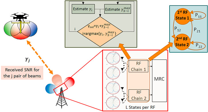
FIGURE 1. The mode of operation of the proposed scheme.

In the following, in order to simplify notations, the time index n is omitted. Assuming independence among the received SNRs from the two RFs at the GS, the MGF of ${\gamma }_{\text{out}}$ is given by

$M_{{\gamma }_{\text{out}}}\left(s\right)={\displaystyle \sum }_{i=1}^2{\pi }_i{M}_{{\gamma }_i}\left(s\right)M_{{\gamma }_{\overline{i}}}^{\text{max}}\left(s\right),(2)$

where $M_X\left(s\right)$ denotes the moment generating function (MGF) of random variable (RV) X. The mode of operation of the proposed scheme defines a two-state regular and ergodic Markov chain, which is characterized by a unique and stable vector of stationary probabilities $\mathit{\pi }$$=[{\pi }_1,{\pi }_2]$, i.e., ${\pi }_i$ is the limiting probability that the ith RF chain is employed.

2.2 Channel Model

In UAV-enabled communications, an important parameter that affects the system’s performance is the wireless medium. Most studies in this area are analyzing the path loss behavior between the UAV and the ground, e.g., Al-Hourani et al. (2014). Recently, another important factor related to the radio model was investigated for UAV-enabled communications, i.e. the impact of the composite fading environment, when the multipath fading coexist with shadowing Bithas et al. (2020). The same basic principle is also followed in this paper. In general, UAV-enabled communications are characterised by line-of-sight (LoS) communication conditions. Therefore, in this paper the behavior of the multipath fading amplitude is modeled by the Nakagami-m distribution Simon and Alouini (2005). It is noted that for $m>1$, Nakagami-m distribution can closely approximate the Ricean distribution, which is often used to model LoS propagation conditions, while by setting $m=1$, it coincides with Rayleigh fading, modeling thus non-LoS conditions. Particularly, based on the method of moments, a one-to-one mapping exists between the Nakagami-m fading parameter and the Rice K factor, i.e., $m=\frac{{\left(1+K\right)}^2}{1+2K}$Simon and Alouini (2005). Under these assumptions, the instantaneous received signal-to-noise ratio (SNR) of the selected pair of patterns at RF i can be mathematically expressed as:

$f_{g_i}\left(\gamma |X_i\right)=\frac{m_i^{m_i}}{\text{Γ}\left(m_i\right)X_i^{m_i}}{\gamma }^{m_i-1}\text{exp}\left(-\frac{m_i\gamma }{X_i}\right),(3)$

where $m_i$ is the shaping parameter of the distribution, $X_i$ is the normalized scaling parameter and $\text{Γ}(\cdot )$ denotes the Gamma function (Gradshteyn and Ryzhik, 2000, eq. (8.310/1)). In a non-shadowed communication environment, the mean of the received SNR $X_i$ would be deterministic. However, in several communication scenarios, the LoS assumption is not always satisfied Khuwaja et al. (2018). Under shadowing conditions, the mean envelope levels are randomly varying. In this paper, the random variations of $X_i$ are modeled with the use of the gamma distribution, which has been widely employed for modeling large scale fading behavior Abdi et al. (2001). In this context, the probability density function (PDF) of $X_i$ is given by

$f_{X_i}\left(x\right)=\frac{1}{\text{Γ}\left(k_i\right){\overline{\gamma }}_i^{k_i}}{x}^{k_i-1}\text{exp}\left(-\frac{x}{{\overline{\gamma }}_i}\right),(4)$

where $k_i$ is the shaping parameter and ${\overline{\gamma }}_i$ is the scaling parameter of the distribution. Under these circumstances, the composite fading environment that is born is the generalized K $\left(K_G\right)$, with PDF, cumulative distribution function (CDF), and MGF expressions, respectively given by Bithas et al. (2006).

$f_{{\gamma }_i}\left(\gamma \right)=\frac{1}{\text{Γ}\left(m_i\right)\text{Γ}\left(k_i\right)}{\left(\frac{m_i}{{\overline{\gamma }}_i}\right)}^{\frac{m_i+k_i}{2}}{\gamma }^{\frac{m_i+k_i}{2}-1}{K}_{m_i-k_i}\left(\frac{2\sqrt{m_i\gamma }}{\sqrt{{\overline{\gamma }}_i}}\right),(5)$

$F_{{\gamma }_i}\left(\gamma \right)=1-{\displaystyle \sum }_{i=0}^{m_i-1}\frac{2}{\text{Γ}\left(k_i\right)i!}{\left(\frac{m_i\gamma }{{\overline{\gamma }}_i}\right)}^{\frac{k_i+i}{2}}{K}_{i-k_i}\left(\frac{2\sqrt{m_i\gamma }}{\sqrt{{\overline{\gamma }}_i}}\right),(6)$

$M_{{\gamma }_i}\left(s\right)={\left(\frac{m_i}{{\overline{\gamma }}_{i}s}\right)}^{\frac{m_i+k_i-1}{2}}\text{exp}\left(\frac{m_i}{2{\overline{\gamma }}_{i}s}\right)W_{\frac{1-k_i-m_i}{2},\frac{m_i-k_i}{2}}\left(\frac{m_i}{{\overline{\gamma }}_{i}s}\right).(7)$

In (5), $K_v(\cdot )$ denotes the modified bessel function of the second kind and order v (Gradshteyn and Ryzhik, 2000, eq. (8.407)). In (6), integer values have been assumed for $m_i$, whereas in (7), $W_{\mu ,\nu }(\cdot )$ denotes the Whittaker function (Gradshteyn and Ryzhik, 2000, eq. (9.22/4)).

3 Stochastic Analysis of the Low Complexity Antenna Technique

In this paper, it is assumed that the channels related to all the available beams of a particular Tx-Rx RF chain pair are subjected to fully correlated shadowing, i.e., they are characterized by the same shadowing coefficient. Since, it is expected that the same obstacle will affect all the available pattern pairs identically, such an assumption can be considered as reasonable. This is why it has been also adopted by various researchers in the past, e.g., Zhu et al. (2010); Bithas and Rontogiannis (2015). Moreover, for the evaluation of the MGF of ${\gamma }_{\text{out}}$, the MGF of $M_{{\gamma }_i}^{\text{max}}\left(s\right)$ is required to be obtained.

Theorem 3.1. Let${\gamma }_i^{\text{max}}$denote a RV, defined as follows

${\gamma }_i^{\text{max}}=\text{max}\left\{g_1{X}_i,g_2{X}_i,\cdots ,g_M{X}_i\right\}=\underset{G_{\text{max}}}{\underbrace{\text{max}\left\{g_1,g_2,\cdots ,g_M\right\}}}{X}_i.(8)$

The PDF and the CDF of ${\gamma }_i^{\text{max}}$ are, respectively, given by

$\begin{array}{c}{f}_{{\gamma }_i^{\text{max}}}\left(\gamma \right)={\displaystyle \sum }_{n=1}^M\left(\begin{array}{c}M\\ n\end{array}\right){\left(-1\right)}^n\underset{i_0+i_1+\cdots +i_{m_i-1}=n}{{\displaystyle \sum }_{i_0=0}^n{\displaystyle \sum }_{i_1=0}^n\cdots {\displaystyle \sum }_{i_{m_i-1}=0}^n}\frac{2n!}{i_0!i_1!\cdots i_{m_i-1}!}\left({\displaystyle \prod }_{j=1}^{m_j-1}\frac{1}{j^{i_j}}\right)\frac{m_i^{{\xi }_i^{+}}}{\text{Γ}\left(k_i\right){\overline{\gamma }}_i^{k_i}}\\ \times {\left(\frac{1}{{\overline{\gamma }}_i{{\displaystyle \sum }}_{j=0}^{m_i-1}{i}_j}\right)}^{{\xi }_i^{-}}[\left({\displaystyle \sum _{j=1}^{m_i-1}j{i}_j}\right)x^{{\xi }_i^{+}-1}{K}_{2{\xi }_i^{-}}\left(\frac{2\sqrt{k_j{\displaystyle {\sum }_{j=0}^{m_j-1}{i}_j}}}{\sqrt{{\overline{\gamma }}_i}}{\gamma }^{1/2}\right)\\ -m_i{\left(\frac{{\displaystyle {\sum }_{j=0}^{m_i-1}{i}_j}}{m_i{\overline{\gamma }}_i}\right)}^{1/2}{x}^{{\xi }_i^{+}-1/2}{K}_{1+2{\xi }_i^{-}}\left(\frac{2\sqrt{k_j{\displaystyle {\sum }_{j=0}^{m_j-1}{i}_j}}}{\sqrt{{\overline{\gamma }}_i}}{\gamma }^{1/2}\right)]\end{array}(9)$

and

$\begin{array}{c}{F}_{{\gamma }_i^{\text{max}}}\left(\gamma \right)=1+{\displaystyle \sum }_{n=1}^M\left(\begin{array}{c}M\\ n\end{array}\right){\left(-1\right)}^n\underset{i_0+i_1+\cdots +i_{m_i-1}=n}{{\displaystyle \sum }_{i_0=0}^n{\displaystyle \sum }_{i_0=0}^n\cdots {\displaystyle \sum }_{i_{m_i-1}=0}^n}\frac{2n!}{i_0!i_1!\cdots i_{m_i-1}!}\left({\displaystyle \prod }_{j=1}^{m_j-1}\frac{1}{j^{i_j}}\right)\frac{{\left(m_i\gamma \right)}^{{\xi }_i^{+}}}{\text{Γ}\left(k_i\right){\overline{\gamma }}_i^{k_i}}\\ \times {\left(\frac{1}{{\overline{\gamma }}_i{{\displaystyle \sum }}_{j=0}^{m_i-1}\hspace{0.17em}{i}_j}\right)}^{{\xi }_i^{-}}{K}_{2{\xi }_i^{-}}\left(\frac{2\sqrt{k_j{{\displaystyle \sum }}_{j=0}^{m_j-1}\hspace{0.17em}{i}_j}}{\sqrt{{\overline{\gamma }}_i}}{\gamma }^{1/2}\right)\end{array},(10)$

where ${\xi }_i^{\pm }=\frac{\pm k_i+{{{\displaystyle \sum }}^{\text{}}}_{j=1}^{m_i-1}j{i}_j}{2}$.

ProofSee the Appendix.

Corollary 3.1.1. The MGF of${\gamma }_i^{\text{max}}$is given by:

$\begin{array}{c}{M}_{{\gamma }_i^{\text{max}}}\left(s\right)={\displaystyle \sum }_{n=1}^M\left(\begin{array}{c}M\\ n\end{array}\right){\left(-1\right)}^n\underset{i_0+i_1+\cdots +i_{m_i-1}=n}{{\displaystyle \sum }_{i_0=0}^n{\displaystyle \sum }_{i_1=0}^n\cdots {\displaystyle \sum }_{i_{m_i-1}=0}^n}\frac{n!}{i_0!i_1!\cdots i_{m_i-1}!}{\left({\displaystyle \prod }_{j=0}^{m_j-1}\frac{1}{i_j}\right)}^{{\xi }_i^{-}+\frac{1}{2}}{\left(\frac{m_i}{{\overline{\gamma }}_i}\right)}^{{\xi }_i^{+}-\frac{1}{2}}\\ \times {\left(\frac{1}{{{\displaystyle \sum }}_{j=0}^{m_i-1}\hspace{0.17em}{i}_j}\right)}^{{\xi }_i^{-}+\frac{1}{2}}\frac{\text{Γ}\left({{\displaystyle \sum }}_{j=0}^{m_i-1}\hspace{0.17em}j{i}_j+1\right)}{s^{{\xi }_i^{+}}}\text{exp}\left(\frac{m_i{{\displaystyle \sum }}_{j=0}^{m_i-1}{i}_j}{2{\overline{\gamma }}_{i}s}\right)\\ \times \left[s^{1/2}{W}_{1/2-{\xi }_i^{+},{\xi }_i^{-}}\left(\frac{m_i{{\displaystyle \sum }}_{j=0}^{m_j-1}{i}_j}{{\overline{\gamma }}_{i}s}\right)-m_i{\left(\frac{{{\displaystyle \sum }}_{j=0}^{m_i-1}{i}_j}{m_i{\overline{\gamma }}_i}\right)}^{1/2}{W}_{-{\xi }_i^{+},{\xi }_i^{-}+1/2}\left(\frac{m_i{{\displaystyle \sum }}_{j=0}^{m_j-1}{i}_j}{{\overline{\gamma }}_{i}s}\right)\right].\end{array}(11)$

Proof. By substituting (9) in the definition of the MGF, making a change of variables, using (Gradshteyn and Ryzhik, 2000, eq. (6.63)), and after some mathematical simplifications, finally yields (11).

For the special case where small scale fading conditions are characterized by Rayleigh distribution, (11) simplifies to the following expression

$\begin{array}{c}{M}_{{\gamma }_i^{\text{max}}}\left(s\right)={\left(\frac{1}{{\overline{\gamma }}_{i}s}\right)}^{\frac{k_i}{2}}\text{exp}\left(\frac{1}{2{\overline{\gamma }}_{i}s}\right)W_{\frac{-k_i}{2},\frac{k_i-1}{2}}\left(\frac{1}{{\overline{\gamma }}_{i}s}\right){\displaystyle \sum }_{j=1}^M\left(\begin{array}{c}M\\ j\end{array}\right){\left(-1\right)}^{j+1}{\left(\frac{j}{s{\overline{\gamma }}_{3-i}}\right)}^{\frac{k_{3-i}}{2}}\\ \times \text{exp}\left(\frac{j}{2s{\overline{\gamma }}_{3-i}}\right)W_{\frac{-k_{3-i}}{2},\frac{k_{3-i}-1}{2}}\left(\frac{j}{{\overline{\gamma }}_{3-i}s}\right).\end{array}(12)$

3.1 Transition Probabilities

The Markov chain is characterized by stationarity probabilities $\mathit{\pi }=[{\pi }_1,{\pi }_2]$, which can be evaluated by ${\pi }_i=\frac{P_{3-i,i}}{1-P_{i,i}+P_{3-i,i}}$, where $P_{i,j}$, denotes the transition probabilities of the Markov chain. As a result of the mode of operation of the beam selection strategy presented in Section 2, the transition probabilities can be evaluated by:

$\begin{array}{c}{P}_{i,i}=Pr\{{\gamma }_i>{\gamma }_{3-i}^{\text{max}}\}\\ ={{{\displaystyle \int }}^{\text{}}}_0^{\infty }{{{\displaystyle \int }}^{\text{}}}_0^x{f}_{{\gamma }_{3-i}}^{\text{max}}\left(y\right)f_{{\gamma }_i}\left(x\right)dydx.\end{array}(13)$

By substituting (5) and (9) in (13), making a change of variables of the form $z=x^{1/2}$, using (Gradshteyn and Ryzhik, 2000, eq. (6.576/4)), and after some algebra, the following expression for the transition probability is extracted:

$\begin{array}{c}{P}_{i,i}=1+{\displaystyle \sum }_{n=1}^M\left(\begin{array}{c}M\\ n\end{array}\right)\underset{i_0+i_1+\cdots +i_{m_i-1}=n}{{\displaystyle \sum }_{i_0=0}^n{\displaystyle \sum }_{i_1=0}^n\cdots {\displaystyle \sum }_{i_{m_i-1}=0}^n}\frac{{\left(-1\right)}^{n}n!}{i_0!i_1!\cdots i_{m_i-1}!}\left({\displaystyle \prod }_{j=1}^{m_i-1}\frac{1}{{\left(j!\right)}^{i_j}}\right){\left(\frac{1}{{{{\displaystyle \sum }}^{\text{}}}_{j=0}^{m_i-1}{i}_j}\right)}^{m_i+{{{\displaystyle \sum }}^{\text{}}}_{j=0}^{m_i-1}j{i}_i}\\ \times \frac{\text{Γ}\left({{{\displaystyle \sum }}^{\text{}}}_{j=1}^{m_i-1}j{i}_j+m_i\right)\text{Γ}\left(2{\xi }_i^{+}\right)\text{Γ}\left(m_i+k_{3-i}\right)\text{Γ}\left(k_i+k_{3-i}\right)}{\text{Γ}\left(m_i\right)\text{Γ}\left(k_i\right)\text{Γ}\left(k_{3-i}\right)\text{Γ}\left(m_i+k_{3-i}+2{\xi }_i^{+}\right)}{\left(\frac{m_i{\overline{\gamma }}_{3-i}}{{\overline{\gamma }}_i{m}_{3-i}}\right)}^{m_i}\\ {\times }_2{F}_1\left({\displaystyle \sum }_{j=1}^{m_i-1}j{i}_j+m_i,k_{3-i}+m_i;m_i+k_{3-i}+2{\xi }_i^{+};\frac{m_i{\overline{\gamma }}_{3-i}}{m_{3-i}{\overline{\gamma }}_i{{{\displaystyle \sum }}^{\text{}}}_{j=0}^{m_i-1}{i}_j}\right),\end{array}(14)$

where $2^{F_1}(\cdot )$ denotes the Gauss hypergeometric function (Gradshteyn and Ryzhik, 2000, eq. (9.100)). Moreover, assuming Rayleigh fading conditions, (14) simplifies to:

$P_{i,i}=1+{\displaystyle \sum }_{n=1}^M\left(\begin{array}{c}M\\ n\end{array}\right)\frac{{\left(-1\right)}^n{\overline{\gamma }}_{3-i}}{n\text{Γ}\left(k_{3-i}\right){\overline{\gamma }}_i}\frac{\text{Γ}\left(k_{3-i}+1\right)\text{Γ}\left(k_i+k_{3-i}\right)}{\text{Γ}\left(1+k_i+k_{3-i}\right)}{\times }_2{F}_1\left(1,k_{3-i}+1;1+k_i+k_{3-i};1-\frac{{\overline{\gamma }}_{3-i}}{n{\overline{\gamma }}_i}\right).(15)$

It is noted that for $i\ne j,P_{i,j}=1-P_{i,i}$.

3.2 Numerical Results

In this subsection, various numerically evaluated results complemented with simulated ones are presented. In order to approximate non-identically distributed conditions, an exponential model for the average SNRs is adopted as follows: ${\overline{\gamma }}_2={\overline{\gamma }}_1\text{exp}\left(-\delta \right)$, where δ denotes a power decaying factor. In all scenarios investigated, it is assumed that $\delta =0.1$. Moreover, based on (2), (7), (11), and (12), the BER performance of DBPSK modulation scheme has been investigated by using ${\overline{P}}_{\text{be}}=\frac{1}{2}{M}_{{\gamma }_{\text{out}}}\left(1\right)$.

In Figure 2, assuming $L=2$, $m_1=2.5,m_2=1.9$, i.e., good multipath fading conditions, the BER is plotted as a function of the average input SNR of the first RF chain ${\overline{\gamma }}_1$, for various values of the shadowing shaping parameter $k_i$. In this figure, the significant influence of shadowing to the system performance is highlighted. In Figure 3, assuming $L=6$, $k_1=1.2,k_2=1.5$, i.e., moderate shadowing conditions, the BER is plotted as a function of ${\overline{\gamma }}_1$, for different values of the multipath fading shaping parameter $m_i$. The comparison of Figure 3 with Figure 2 can easily verify that the variation of the shadowing conditions has great impact to the system’s performance compared to the variations of the severeness of multipath fading. Finally, in Figure 4, assuming $m_1=2,m_2=2$$k_1=1.2,k_2=1.5$, i.e., moderate fading and shadowing conditions, the BER is plotted as a function of ${\overline{\gamma }}_1$, for various numbers of the available patterns L. For comparison purposes two additional scenarios are also presented: 1) a scenario with MRC reception only, i.e., without the exploitation of the beam selection, and; 2) a pure beam selection scheme from a single Rx-RF chain, based on the maximum selection criterion. The performance improvement due to the proposed approach that combines beam selection and MRC diversity can easily be verified compared to the two simpler approaches. In all cases, Monte Carlo simulations have also been performed and included in the figures, verifying the validity of the proposed approach.

FIGURE 2

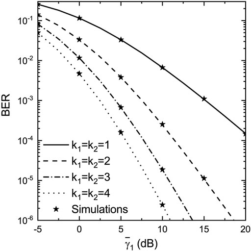
FIGURE 2. BER vs ${\overline{\gamma }}_1$, for different values of $k_i$.

FIGURE 3

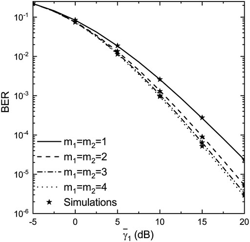
FIGURE 3. BER vs ${\overline{\gamma }}_1$, for different values of $m_i$.

FIGURE 4

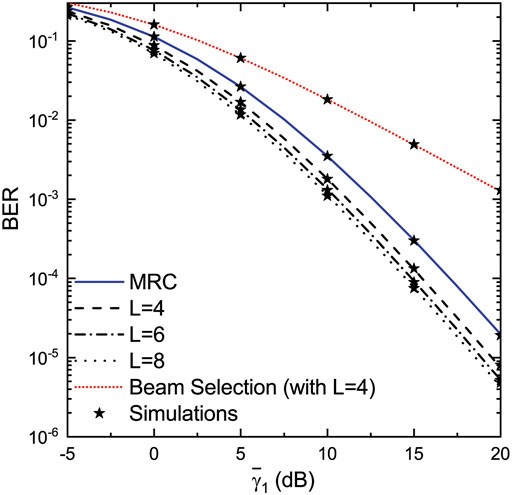
FIGURE 4. BER vs ${\overline{\gamma }}_1$, for different values of L.

4 Low-complexity Implementation of Antenna Pattern Dynamic Configuration Using ESPAR

Up to this point, the analysis is implementation-agnostic and does not consider specific techniques that can be employed in order to use multiple radiation patterns to improve the performance and reliability of UAV links. In this section, a low complexity MIMO implementation of the proposed approach is presented using ESPAR antennas. The ESPARs are able to provide multiple patterns using only one active and many parasitic elements. Pattern reconfigurability is achieved by electronically adjusting the loads of the parasitic elements. The reduction of the number of RF chains and RF electronics, while simultaneously maintaining beamforming capabilities, lead to significant cost and consumed power reduction with no performance degradation.

The antenna pattern of the ESPAR depends on the current flow on all array elements (active and parasitics), as well as the array geometry, which is mathematically expressed through the array manifold vector, i.e., for isotropic radiator elements, the radiation pattern towards angles φ (azimuth) and θ (elevation) is given by:

$P\left(\theta ,\phi \right)={\mathbf{i}}^T\mathbf{a}\left(\theta ,\phi \right),(16)$

where $\mathbf{i}$ denotes the $N\times 1$ vector containing the currents on the N antenna elements–assuming an ESPAR with an active and $\left(N-1\right)$ parasitic elements; and $\mathbf{a}\left(\theta ,\phi \right)$ is the manifold vector. For a planar array, the $m-$th element of the manifold is given by:

${\left[\mathbf{a}\left(\theta ,\phi \right)\right]}_m=a_m\left(\theta ,\phi \right)=\{\begin{array}{cc}1& m=1\\ e^{\frac{2\pi }{\lambda }\left[\begin{array}{ccc}\text{cos}\phi \hspace{0.17em}\text{sin}\theta & \text{sin}\phi \hspace{0.17em}\text{sin}\theta & \text{cos}\theta \end{array}\right]]{\left[\begin{array}{ccc}{x}_m& y_m& z_m\end{array}\right]}^T}& m\ne 1,\end{array}(17)$

where λ is the wavelength. Also, assuming a properly defined coordinate system for the array (usually using the active as the origin), $x_m$, $y_m$ and $z_m$ denote the coordinates of the m-th element.

In the majority of existing studies, the expression of (16) is sufficient, since 2D propagation is considered with the use of half-wavelength elements, i.e., with an omnidirectional pattern at the azimuth plane. When investigating the use of ESPARs for UAV-to-ground links, the elevation pattern of the array becomes crucial, and the pattern of each individual element should be considered for the calculation of the composite pattern, thus:

$P\left(\theta ,\phi \right)={\mathbf{i}}^T\left(\mathbf{p}\left(\theta ,\phi \right)\cdot \mathbf{a}\left(\theta ,\phi \right)\right)(18)$

where $(\cdot )$ notates the Hadamard product and $\mathbf{p}$ is an $N\times 1$ vector containing the pattern values for each array element, i.e., ${\left[\mathbf{p}\left(\theta ,\phi \right)\right]}_m$ is the pattern value of the m-th antenna elements towards angles φ and θ.

In order to control the antenna currents and consequently the produced patterns, we focus on the mutual coupling matrix ${\mathbf{Z}}_{ESPAR}\in {\mathrm{ℂ}}^{N\times N}$ that depends on the array geometry and can be calculated from simulations, measurements or analytical expressions (Balanis (2016), chapter 8). Through the antenna array Thevenin equivalent model (for Tx operation depicted in Figure 5), the current on each element can be extracted by:

$\mathbf{i}={\left({\mathbf{Z}}_{ESPAR}+\mathbf{X}\right)}^{-1}{\mathbf{e}}_1{v}_s,(19)$

where, the active element is considered at the first position of the voltage/current vectors, ${\mathbf{e}}_i$ represents the vector ${\mathbf{e}}_i^T=\left[\begin{array}{ccccc}0& \dots 0& \underset{i-t\text{h position}}{1}& \mathrm{0....}& 0\end{array}\right]$ and $v_s$ is the voltage source at the active element, carrying the actual information signal. Matrix $\mathbf{X}$ is a diagonal matrix containing the loads of all the elements, i.e., $\mathbf{X}=diag\left(\mathbf{x}\right)$, where $\mathbf{x}={\left[\begin{array}{ccccc}{Z}_1& j{X}_2& j{X}_3& \dots & j{X}_N\end{array}\right]}^T$. It is noted that only imaginary loads (varactors) at the parasitics are considered, so that no active power is consumed on them, i.e., $X_2,X_3,\dots ,X_N\in \mathrm{ℝ}$. Matrix $\mathbf{Y}\left(\mathbf{x}\right)={\left({\mathbf{Z}}_{ESPAR}+\mathbf{X}\right)}^{-1}$ is also known as the conductivity matrix.

FIGURE 5

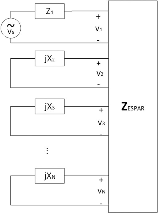
FIGURE 5. Thevenin equivalent for ESPAR Tx operation.

Let’s consider that the ESPAR antenna is installed at the transmitter. Assuming that $\mathbf{w}$ is the beamforming vector controlling the transmission pattern, and n an additive white Gaussian noise term, then the received signal can be modeled by:

$y={\mathbf{h}}^T\mathbf{w}s+n,(20)$

where we consider single-antenna reception (an MISO equivalent setup); s is the transmitted information signal, and $\mathbf{h}\in {\mathrm{ℂ}}^{N\times 1}$ represents the channel vector. If we consider K scatterers defining the radio channel, then:

$\mathbf{h}=\mathbf{A}\tilde{h}(21)$

where $\tilde{h}\in {\mathrm{ℂ}}^{K\times 1}$ is the vector of the complex channel gains of the K scatterers, $\mathbf{A}\in {\mathrm{ℂ}}^{N\times K}$ is the steering matrix extracted by the array manifold, i.e.,

${\left[\mathbf{A}\right]}_{m,k}={\left[\mathbf{a}\left({\theta }_k,{\phi }_k\right)\right]}_m(22)$

which means that $\mathbf{A}$ contains the values from (17) at the Angles of Departure $\left({\theta }_k,{\phi }_k\right)$ from the transmitter to the k-th scatterer. The information signal s is considered dimensionless, however, according to the aforementioned analysis is reciprocal to the source voltage at the transmitter. As it is noted at Section 2, where the pattern selection concept was introduced, the GS supports two RF chains, while the UAV is equipped with one. This means that it is assumed that the GS will consist of two ESPARs applying the aforementioned dynamic scheme, while the UAV will be equipped with one ESPAR. Due to the reciprocity principle, the dynamic pattern adaptation procedures are applicable at both direct (GS as a Tx) and reverse (GS as a Rx) links. It is noted that the following scheme can be straightforwardly extended to configurations that include more active elements and RF chains. Nevertheless, the effectiveness of the ESPAR antenna and the proposed scheme is highlighted by the use of a very low number of RF chains - reducing the cost and complexity of the system.

4.1 An ESPAR for Aerial Communications

The system beamforming capabilities depend heavily on the ESPAR design. More specifically.

• The antenna geometry affects the beamwidth, directivity and beamshaping capabilities. Each element acts as a reflector and shaper of the pattern. For example, in order to increase gain towards a direction, elements have to be placed behind the active to act as reflectors, while in order to steer the patterns, one or more elements should be used in front of the active, as regulators.

• The inter-element distance controls the coupling among active and parasitic elements. Close inter-element distances lead to designs with high gains, however, due to increased correlation beamshaping requires higher parasitic load values.

• The parasitic antenna element length causes variations on the mutual coupling values in ${\mathbf{Z}}_{ESPAR}$ and consequently influence the pattern capabilities of the antenna.

• The range of the possible varactor values of the parasitics limits the steering/shaping capabilities of the antenna.

In this paper, several geometries and inter-element distances were investigated. The varactor load range was selected to be feasible and implementable $\left([-5\text{kΩ},5\text{kΩ}]\right)$. For simplicity, all antenna elements were assumed identical. The design of the ESPAR for the investigated use case is based on the following objectives:

• To be able to provide a large set of available radiation patterns;

• To consist of simple half-wavelength dipole elements, that considerably simplify the analysis - and avoid complicated EM solvers. Nevertheless, the dipoles are not considered ideal for aerial communications due to their constraint support over the elevation plane;

• To be able to provide significantly increased beamwidth over the elevation plane despite the fact that it consists of simple dipoles;

• With a pair of tilted ESPARs at the GS, to be able to provide full support over the circular sector covered by the GS, i.e., it is able to reconfigure in order to track a UAV moving at any possible angle $\phi \in \left(0,\pi \right),\theta \in \left(0,\frac{\pi }{2}\right)$, assuming that the antenna orientation is towards $\phi =\pi /2$. It is noted that more RF chains can be added in a straightforward fashion, so that performance can be improved. However, a significant benefit of the ESPAR is that a small number of RF chains is sufficient to outperform conventional schemes with many actives. As an example, it is shown that two RF chains are enough to outperform conventional 8-element beamformers;

• To offer significant gain and directivity to a wide range of angles at both azimuth and elevation planes, and in conjunction to the previous point, to be able to reconfigure the pattern and provide gain greater than the maximum of the plain $\lambda /2$ dipole (2.15 dB) at all probable angles - even for $\theta =0$.

Several ESPAR antenna geometries were tested through simulation in terms of directivity, beam steering support and flexible beamwidths. The geometry of the ESPAR antenna that was able to fulfill all the requirements is presented in Figure 6, while the element coordinates are provided in Table 1, where $d=\lambda /4$. All elements are $\lambda /2$-dipoles.

FIGURE 6

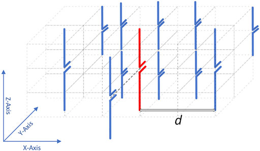
FIGURE 6. The ESPAR geometry (single active, 11 parasitics) designed for aerial communications. The active element is in red color.

TABLE 1

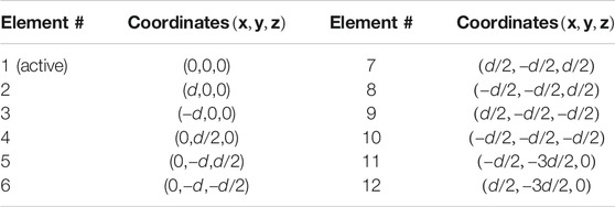
TABLE 1. Cartesian coordinates of the antenna elements using the active as reference.

The following notes can be made on the designed ESPAR:

• The antenna is implemented with the objective to provide improved directivity over the range $\theta \in [0,\pi )$. Thus, the majority of passive elements is placed “behind” the active, in order to use them as reflectors and as a tracking mechanism.

• A single passive is placed “in front” of the active (Element # 4). The role of this element is to balance the generated patterns more accurately to the targets, and also provide limited but substantial support over the range $\theta \in [\pi ,2\pi )$.

• The elements are placed in three vertical layers over a parallelepiped grid. Co-linear placement of the elements improves the elevation plane support of the generated patterns.

Despite our attempt to design an array with optimized directivity over the elevation plane, the vertical dipole elements cannot generate patterns to provide significant gain at low θ angles. In order to tackle this drawback at the GSs, the assumed ESPARs are positioned according to the layout presented in Figure 7. Based on this layout, the two ESPARs are placed vertically, while the distance D between them is several wavelengths. The two antennas are tilted (on z-axis) by two different angles ${\theta }_A$ and ${\theta }_B$. The relatively high separation distance D ensures spatially uncorrelated reception by the two arrays, while the assumption for common shadowing remains valid. The tilt angles are chosen so that 1) they ensure full support over the circular sector of interest; 2) maximize gain and directivity at the range of angles where the UAVs are expected to operate.

FIGURE 7

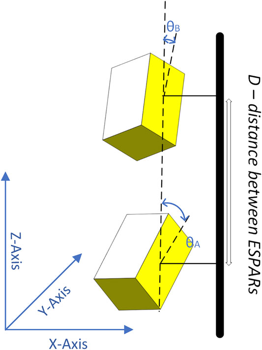
FIGURE 7. The layout of the two ESPARs at the GS.

An example of the performance of the antenna is given in Figure 8A and Figure 8B. In this example, we assume a sole cluster of $K=10$ scatterers located near the direction $\left(\phi =\pi /4,\theta =\pi /4\right)$. The azimuth orientation of the two antenna arrays is towards $\phi =\pi /2$, the separation distance was set to $D=3\lambda$ and the tilts were ${\theta }_A=\pi /4$ and ${\theta }_B=\pi /12$. The channel for each ESPAR is calculated by (21), taking also into account the phase difference due to the separation of the arrays by D.

FIGURE 8

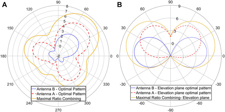
FIGURE 8. 1) Selected patterns for each ESPAR and combined pattern for a cluster of scatterers at $\left(\phi =\pi /4,\theta =\pi /4\right)$ - Azimuth plane (in dB), 2) Selected patterns for each ESPAR and combined pattern for a cluster of scatterers at $\left(\phi =\pi /4,\theta =\pi /4\right)$ - Elevation plane (in dB).

The beamforming algorithm (analyzed in Subsection 4.2) is then used in order to select the patterns for SNR maximization towards the specific direction. The reception is concluded with maximal ratio combining (MRC) of the received signals from the two active elements of the arrays. In case more active elements are used, MRC is performed over the available set Figure 8A presents the resulted radiation patterns at the azimuth plane, while Figure 8B presents the patterns at the elevation plane. It becomes clear, that the beamformers clearly concentrate the beams towards the specific direction at the best of their ability. Due to the difference in the array tilts, Antenna A is dominating the specific link and the overall gain of the combined reception exceeds 7 dB.

In order to validate that the antenna satisfies the requirements that were set during the design process, the above experiment was repeated for all angles defined in pairs over the circular sector of interest ($\phi \in \left(0,\pi \right),\theta \in \left(0,\frac{\pi }{2}\right)$). The resulted polarplots are presented in Figures 9A,B and Figure 10. It is noted that the presented polarplots are not radiation patterns, but they depict the achieved gain per direction after shaping the beam towards the direction through the beamforming process. In Figure 9A, the achieved gain per direction in the azimuth plane for $\theta =\pi /4$ is presented, while Figure 9B presents the achieved gain per direction in the elevation plane for $\phi =\pi /4$. Finally, Figure 10 provides a 3D display of the results for the circular sector of interest.

FIGURE 9

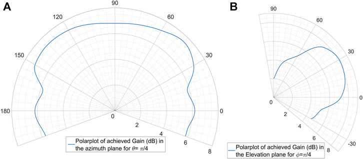
FIGURE 9. 1) Polarplot of the achieved gains (in dB) through beamforming per azimuth angle $\phi \in [-\mathrm{20,200}]$ and for $\theta =45$°; 2) Polarplot of the achieved gains (in dB) through beamforming per elevation angle $\theta \in [-\mathrm{30,90}]$ and for $\phi =45$°.

FIGURE 10

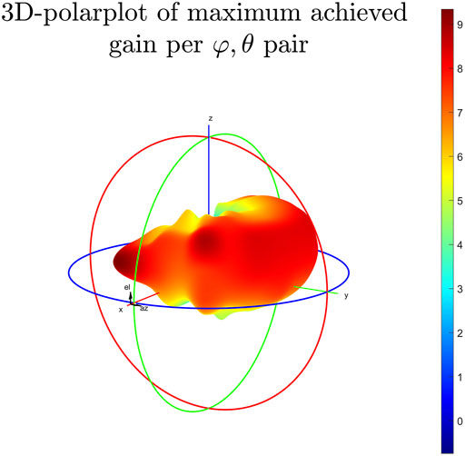
FIGURE 10. 3D - Polarplot of the achieved gains (in dB) through beamforming per angle pair ($\phi \in [-\mathrm{20,200}]$ and $\theta \in [-\mathrm{30,90}]$°).

4.2 Pattern Reconfiguration - Beamforming

This subsection presents all the steps of the radiation pattern reconfiguration process for the aforementioned antenna system. We focus on the reconfiguration strategy at the GS. According to the scheme presented in Sec. 2.1, a typical operational scenario is presented below:

• The UAV is equipped with an ESPAR (Figure 6), while the GS is equipped with two ESPARs in the layout presented in Figure 7. The UAV ESPAR is assumed tilted down ($\theta =\pi /4$).

• Both systems are able to reconfigure their patterns by tuning the varactor loads of the parasitic elements. If the parasitic loads are able to take specific quantized values, a finite set of available patterns per antenna is defined.

• A UAV is moving at the circular sector monitored by the GS. Using the channel estimates, the UAV estimates and selects the pattern that is expected to perform optimally for the specific radio channel.

• Since, the GS has two arrays, it maintains the pattern of the one array (the one with the better SNR performance) and performs dynamic reconfiguration for the other array in order to optimize the link.

• In all cases, the reception is completed with MRC from the two arrays, and the transmission is performed equivalently with maximal ratio transmission (MRT).

4.2.1 Beamforming at the ESPAR

The first part of the methodology is to propose a beamforming scheme that can be applied to each ESPAR antenna, with the objective to adapt the radiation pattern in an attempt to optimally exploit the radio channel. Assuming quantized parasitic loads, this is an integer programming problem. However, due to the possibly high number of feasible patterns, we use relaxation of the problem to the continuous equivalent ($X_i\in \mathrm{ℝ}$). The presented methodology is applied at the ESPAR, every time the system performs a search in order to select a different pattern, i.e. anytime the UAV adapts its pattern, or anytime the GS changes the pattern at one of its antennas of Figure 7.

From (19), (20), and (21), it can be concluded that beamforming/beamshaping with ESPARs is achieved by defining $\mathbf{w}$ as follows:

$\mathbf{w}=\frac{1}{c}{\left({\mathbf{Z}}_{ESPAR}+\mathbf{X}\right)}^{-1}{\mathbf{e}}_1,(23)$

where c is a normalization factor. Eq. (23) reveals several challenges in the manipulation of system currents in order to control the reconfigurable radiation pattern:

• The relationship between the beamforming vector and the varactor (i.e., the purely imaginary loads) values is non-linear.

• Matrix $\mathbf{X}$ also contains the matching impedance of the active element.

• If we use conventional techniques in order to estimate desired/optimal beamforming gains, it may not be straightforward to calculate the varactor values, i.e. the matrix $\mathbf{X}$.

In Bucheli Garcia et al. (2020), the problem is solved through linearization achieved through a series of assumptions that may introduce significant estimation errors, as the number of parasitics and the range of varactor values increase. However, the proposed approach and system model presents significant benefits and insights, and therefore is adopted in our work. Initially, in Bucheli Garcia et al. (2020), the resistance of the active is untangled by $\mathbf{X}$, since it should not be part of the optimization process but it should be defined to match the input impedance at the active. Let’s assume that:

$\begin{array}{c}\mathbf{X}=diag\left(\mathbf{x}\right),\\ \mathbf{x}={\left[\begin{array}{ccccc}{Z}_1& j{X}_2& j{X}_3& \dots & j{X}_N\end{array}\right]}^T,\\ \mathbf{X}\prime =jdiag\left(\mathbf{x}\prime \right),\\ \mathbf{x}\prime ={\left[\begin{array}{ccccc}0& X_2& X_3& \dots & X_N\end{array}\right]}^T,\end{array}(24)$

which means that, $\mathbf{X}=j\mathbf{X}\prime +Z_1{\mathbf{e}}_1{\mathbf{e}}_1^T$. With the use of the Woodburry inverse matrix lemma one may calculate the conductivity matrix $\mathbf{Y}\left(\mathbf{X}\right)$ of the array as a function of the conductivity matrix $\mathbf{Y}\left(\mathbf{X}\prime \right)$, that contains only the independent variables of the problem (the varactor loads). The result is given in:

$\mathbf{Y}\left(\mathbf{X}\right)=\mathbf{Y}\left(\mathbf{X}\prime \right)\left({\mathbf{I}}_N-\frac{Z_1\left[\frac{{\left[\mathbf{Y}{\left(\mathbf{X}\prime \right)}^T\right]}_1^T}{0_{\left(N-1\right)\times N}}\right]}{1+Z_1{\psi }_{\mathrm{1,1}}\left(\mathbf{x}\prime \right)}\right)(25)$

where ${\psi }_{\mathrm{1,1}}\left(\mathbf{x}\prime \right)={\left[\mathbf{Y}\left(\mathbf{X}\prime \right)\right]}_{\mathrm{1,1}}={\mathbf{e}}_1^T\mathbf{Y}\left(\mathbf{X}\prime \right){\mathbf{e}}_1$. From (23), it is clear that only the first column of the matrix is required, since ${\left[\mathbf{Y}\left(\mathbf{X}\right)\right]}_1={\left({\mathbf{Z}}_{ESPAR}+\mathbf{X}\right)}^{-1}{\mathbf{e}}_1$, and thus:

${\left[\mathbf{Y}\left(\mathbf{X}\right)\right]}_1={\left[\mathbf{Y}\left(\mathbf{X}\prime \right)\right]}_1\frac{1}{1+Z_1{\psi }_{\mathrm{1,1}}\left(\mathbf{x}\prime \right)}.(26)$

As a next step, and according to (23) and (26), any change on the varactors of the passive elements will cause change of $v_1$ at the output of the active, as presented in Figure 5. The impedance of the active has to be matched with the input impedance at the active, i.e.,

$Z_1=Z_{\text{in}}^{\text{*}}={\left(\frac{v_1}{i_1}\right)}^{\text{*}}={\left(\frac{{\mathbf{e}}_1^T{\mathbf{Z}}_{ESPAR}\mathbf{Y}\left(\mathbf{x}\prime \right){\mathbf{e}}_1}{{\psi }_{\mathrm{1,1}}\left(\mathbf{x}\prime \right)}\right)}^{\text{*}}.(27)$

However, interestingly, since $\left({\mathbf{Z}}_{ESPAR}+\mathbf{X}\prime \right)\mathbf{Y}\left(\mathbf{x}\prime \right)=\mathbf{I}$ , the expression is furtherly simplified, leading to:

$Z_1=Z_{\text{in}}^{\text{*}}={\left(\frac{1}{{\psi }_{\mathrm{1,1}}\left(\mathbf{x}\prime \right)}\right)}^{\text{*}}(28)$

${\left[\mathbf{Y}\left(\mathbf{X}\right)\right]}_1={\left[\mathbf{Y}\left(\mathbf{X}\prime \right)\right]}_1\frac{{\psi }_{\mathrm{1,1}}^{\text{*}}\left(\mathbf{x}\prime \right)}{2\text{Re}\left({\psi }_{\mathrm{1,1}}\left(\mathbf{x}\prime \right)\right)}.(29)$

and from (26), we have:

The previous analysis provides the value of the matched load of the active, while removing it from the beamforming calculation.

In Bucheli Garcia et al. (2020), the authors achieved to provide through a series of approximations a closed expression for the calculation of the beamforming gains:

$\mathbf{w}\approx \frac{{\mathbf{Z}}_{ESPAR}^{-1}{\mathbf{e}}_1}{\sqrt{\text{Re}\left({\left[{\mathbf{Z}}_{ESPAR}^{-1}\right]}_{\mathrm{1,1}}\right)}}+j\frac{{\mathbf{Z}}_{ESPAR}^{-1}diag\left({\mathbf{Z}}_{ESPAR}^{-1}{\mathbf{e}}_1\right)}{\sqrt{\text{Re}\left({\left[{\mathbf{Z}}_{ESPAR}^{-1}\right]}_{\mathrm{1,1}}\right)}}\mathbf{x}\prime .(30)$

The approximation error is reciprocal to ${\left|\left|{\mathbf{Z}}_{ESPAR}^{-1}\mathbf{X}\right|\right|}_F$ and, thus it is desired to minimize this Frobenius norm. This fact, however, sets constraints on the quality of the beamforming with the use of the approximation, since:

• High values of the reactance will also increase the Frobenius norm,

• The existence of many parasitic elements will also unavoidably increase the norm.

Experimentation indicated that for the UAV case, it is necessary to include many parasitics for increased gain and support, and also that high varactance values are necessary in order to ensure that the superposition of the radiated signals by the parasitic elements is beneficial for the resultant pattern in terms of gain and directivity. Therefore, the approximation error was very high and no significant benefit from the use of ESPARs occurred.

In this paper, a new low-complexity method is introduced in order to calculate the values of $\mathbf{x}$ that provide an approximation of the optimal beamforming values. The method is implemented with the following four-step procedure:

Step 1: It is a preparatory step that is performed offline. Initially, we consider that the parasitic loads are uncorrelated random variables. Monte-Carlo simulation is performed, where the value for each load is drawn randomly from a range of values, using an assumed distribution. Then, (23) is used in order to calculate vector $\mathbf{w}$ and estimate its statistics (i.e. mean ${\mathbf{m}}_w$ and covariance matrix ${\mathbf{C}}_w$). The tests were performed assuming that $X_i\in [-5\text{kΩ},5\text{kΩ}]$ following a uniform or Gaussian distribution ($\sigma =1.5\text{kΩ}$). After the execution of many iterations, we are able to estimate ${\mathbf{C}}_w$ and perform Cholesky decomposition i.e., matrix $\mathbf{L}$ is calculated where ${\mathbf{C}}_w=\mathbf{L}{\mathbf{L}}^H$.

Step 2: The reciprocal problem is assumed, where the ESPAR is used for reception. In this case, the transmission model of (20) is transformed to the receiver equivalent $y={\mathbf{w}}^H\mathbf{h}s+n$, where complex conjugation of $\mathbf{w}$ is used to mathematically model the fact that the direction of arrival at the receiver is opposite to the direction of departure. The concept behind the algorithm is that instead of performing computationally-cumbersome non-linear optimization for the selection of $\mathbf{x}$ that optimizes SNR, or equivalently maximizes $\left(|\mathbf{w}{\left(\mathbf{x}\right)}^H\mathbf{h}{|}^2\right)$, optimization is performed over $\mathbf{w}$ and then we numerically calculate the vector $\mathbf{x}$ that produces the weight vector $\mathbf{w}$. However, the problem is that due to its non-linear dependence on $\mathbf{x}$, the solution for $\mathbf{w}$ may not be achievable for any feasible or realistic $\mathbf{x}$. In order to bypass this issue:

• We define a substitute variable, as follows:

$\mathbf{w}={\mathbf{L}}^{-1}\tilde{w}+{\mathbf{m}}_w\Rightarrow \tilde{w}=\mathbf{L}\left(\mathbf{w}-{\mathbf{m}}_w\right)(31)$

• According to the previous approach, if we consider $\mathbf{w}$ as a random variable, then (31) performs whitening and the substitute variable $\tilde{w}$ is a zero-mean, white random variable.

• The vector $\tilde{h}={\mathbf{L}}^{-H}\mathbf{h}$ is defined.

• The initial optimization problem, from

$\begin{array}{l}\text{arg}\underset{\mathbf{w}}{\text{max}}\left(|{\mathbf{w}}^H\mathbf{h}{|}^2\right)\\ \text{s}.\text{t}.{\mathbf{w}}^H\mathbf{w}\mathrm{⩽}{c}^2\end{array}(32)$

Is transformed to the equivalent problem:

$\begin{array}{l}\text{arg}\underset{\tilde{w}}{\text{max}}\underset{\text{s}.\text{t}.{\tilde{w}}^H\tilde{w}\mathrm{⩽}{\tilde{c}}^2}{\left({\left(\tilde{w}+\underset{\mathbf{a}}{\underbrace{\mathbf{L}{\mathbf{m}}_w}}\right)}^H\underset{\tilde{H}}{\underbrace{\tilde{h}{\tilde{h}}^H}}\left(\tilde{w}+\underset{\mathbf{a}}{\underbrace{\mathbf{L}{\mathbf{m}}_w}}\right)\right)}\end{array}(33)$

The constraint $c^2$ bounds the power of $\mathbf{w}$. Due to the fact that in (23), $\mathbf{w}$ is normalized (so that ${\left[\mathbf{w}\right]}_1=1$), and the substitute variable is zero-mean with unitary variance, the constraint in the transformed optimization problem can be expressed as ${\tilde{c}}^2=N$. The transformed optimization problem can be solved with the method of Lagrange multipliers, i.e.:

$\begin{array}{c}\mathrm{ℒ}\left(\tilde{w}\right)={\left(\tilde{w}+\mathbf{a}\right)}^H\tilde{H}\left(\tilde{w}+\mathbf{a}\right)+\mu \left(N-{\tilde{w}}^H\tilde{w}\right)\\ \nabla \mathrm{ℒ}\left(\tilde{w}\right)=\left(\tilde{H}-\mu {\mathbf{I}}_N\right)\tilde{w}+\tilde{H}\mathbf{a}=0,\end{array}(34)$

where the complex gradient for real-valued functions $(\nabla f(z=\alpha +j\beta )=\frac{\partial f\left(z\right)}{\partial \alpha }+j\frac{\partial f\left(z\right)}{\partial \beta })$ is used, and ${\mathbf{I}}_N$ is the $N\times N$ identity matrix. The optimal solution for the transformed problem is given by:

$\widehat{\tilde{w}}=\left(\mu {\mathbf{I}}_N-\tilde{H}\right)\tilde{H}\mathbf{a}(35)$

Then, the beamforming gains are calculated from: $\widehat{w}={\mathbf{L}}^{-1}\widehat{\overline{w}}+{\mathbf{m}}_w$. This correlating process, mathematically produces the beamformer for channel vector $\mathbf{h}$ instead of $\tilde{h}$. and introduces correlation among the elements of $\mathbf{w}$ according to the covariance matrix ${\mathbf{C}}_w$.

Step 3: The next step is to numerically solve (23) and use $\widehat{w}$ to calculate $\widehat{x}$. In our experiments, we used the Trust-Region method implemented in MATLAB through the function fmincon. The performed mathematical trick uses matrix $\mathbf{L}$ to ”shape” the solution $\widehat{w}$ in an attempt to significantly increase the possibility, that the solution results in the feasible range of values of $\widehat{x}$. It should be emphasized, that the algorithm does not always converge to the global optimum and that in several cases, there is no feasible $\widehat{x}$ for a given $\widehat{w}$. In these cases, the value $\widehat{x}=\text{arg}\underset{\mathbf{x}}{\text{min}}\left(|\mathbf{w}\left(\mathbf{x}\right)-\widehat{w}{|}^2\right)$ is selected. However, this mathematical trick produces a result that, in many cases, successfully approximates the optimum, and provides significantly improved results even when there is no convergence.

Step 4: As mentioned before, the varactance values are quantized and there is a discrete, finite set of supported vectors. Let’s assume that the set $\text{X}$ of supported varactance vectors contains M elements ($\text{X}=\left\{{\mathbf{x}}_0,{\mathbf{x}}_1,{\mathbf{x}}_2,\dots {\mathbf{x}}_M\right\}$). The index i of the varactance vector that is chosen, is extracted by finding the vector ${\mathbf{x}}_i$ closest to $\widehat{x}$, i.e., $i=\text{arg}\underset{k}{\text{min}}\left(|{\mathbf{x}}_k-\widehat{x}{|}^2\right)$. The search in Step 4 can be merged with the process described at Step 3.

4.2.2 Pattern Adaptation at the GS

The pattern adaptation process at the GS is presented in Figure 11. The operation of the dynamic adaptation process can be described with the following narrative: Initially, and if no link is established, the system initializes by selecting two near-omnidirectional patterns, since there is no specific radio channel to adapt on. With the establishment of a link, communication between the UAV and the ground is initiated. Periodically, or through an event-based trigger (e.g. very low signal quality), the system selects the antenna i ($i\in \mathrm{1,2})$ that currently showcases the worst performance in terms of SNR. The beamforming algorithm is applied, and a new pattern is selected that is expected to exhibit better performance under the current channel conditions and the UAV position. The pattern of the other antenna remains unmodified in order to reduce complexity, ping-pong effects, and reliability risks. After pattern reconfiguration, transmission is performed with MRT beamforming and reception is performed with MRC over the two arrays. The scheme can be directly extended for schemes with more RF chains available for transmission/reception. It is noted that, since the two arrays are spatially uncorrelated, the pattern adaptation process is independent for each array, and Maximal Ratio techniques provide the best transmission/reception in terms of SNR under the specific conditions.

FIGURE 11

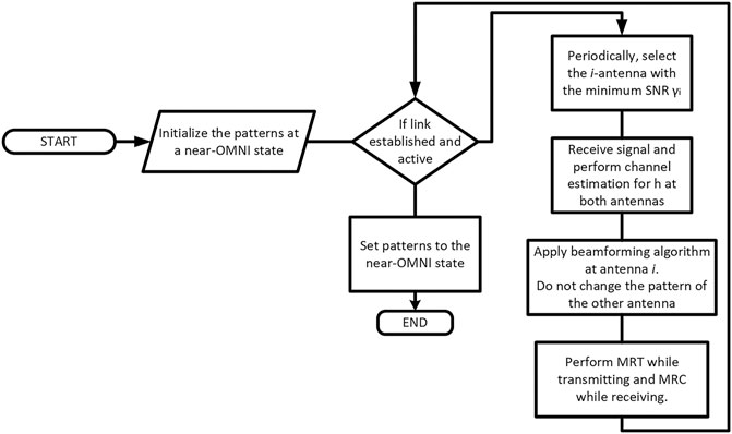
FIGURE 11. The pattern adaptation flow diagram at the GS.

4.3 Numerical Results

A simulator was developed in order to test the system performance. We used the Quadriga Channel Model for Urban Non Terrestrial Networks (Jaeckel et al. (2014); Jaeckel et al. (2016)). Since it is not calibrated for UAV-to-ground communications, modifications were performed mainly in the calculation of pathloss and shadowing for relatively low-altitude drones. The results in (Amorim et al. (2017)) and (Wang et al. (2017)) were exploited, in order to integrate UAV-to-ground communication, as well as, a corrective factor from the 3GPP model (TR38.901 (2018)) was included in order to support multiple frequency bands.

Additionally, some modification in the Quadriga code was necessary in order to be able to use the custom patterns of the ESPARs in the geometric-stochastic layout. S-band transmission was simulated (2.5 GHz), and Time Division Duplex communication between the nodes was assumed. In order to estimate the performance, QPSK signals were transmitted with 1/2-convolutional coding. Perfect channel estimation was assumed. Transmission power was set at 23 dBm.

During the simulation, the UAV is assumed to move at heights ranging from 60 to 120 m from the ground, randomly defined for each run. The distance between the GS and the UAV varies as a uniform random variable, from 120 m to 20 km.

Four configurations were tested:

• Two dipole antennas at the GS (tilted at $\theta =\pi /4$) and one dipole on the UAV (tilted at $\theta =-\pi /4$)

• Two ESPARs at the GS in the layout of Figure 7, where:

• The dynamic pattern adaptation is applied

• The dynamic pattern adaptation with use of Bucheli Garcia et al. (2020) for the beamforming algorithm at the ESAPR is applied

• The optimum pattern selector/beamformer is applied. In this case, brute force optimization is performed over the available patterns. This solution is computationally exhaustive and it is used as a reference.

Results are presented in Figures 12, 13. It can be clearly seen that the dynamic pattern reconfiguration algorithm provides significant enhancement in terms of both capacity/spectral efficiency, as well as in coverage and outage propabilities. Additionally, the performance of the algorithm is quite close to the optimal, exhaustive pattern selection scheme. Indicatively, at 50% percentage, spectral efficiency is approximately 6 bps/Hz, while with use of the dynamic pattern reconfiguration scheme efficiency of 8 bps/Hz is achieved (optimum is 8.5 bps/Hz).

FIGURE 12

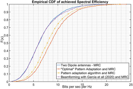
FIGURE 12. Spectral Efficiency for various scenarios - simple dipoles, optimal beamformer, dynamic pattern reconfiguration algorithm, algorithm based on Bucheli Garcia et al. (2020).

FIGURE 13

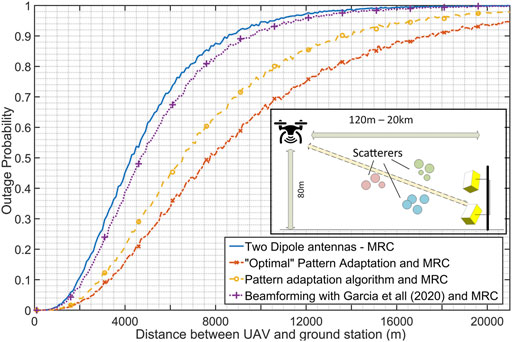
FIGURE 13. Outage Probability vs. distance for the tested scenarios.

As far as coverage is concerned, in Figure 13, the outage probability vs. the UAV-GS distance is presented. More than 5,000 simulation runs were executed, where the UAV height was set to 80 m, and its distance from the GS varies randomly from 120 m to 20 km. Packets of 32 bytes were simulated in a link-level setup, using the aforementioned modulation scheme. Outage probability is calculated by measuring the packet error rate. The results indicate that at 6 km, the outage probability is 20% for the plain dipole configuration, while with dynamic pattern reconfiguration from a finite set of patterns, it decreases to 8%. The optimal pattern reduces the outage furtherly at 5%. The proposed pattern adaptation algorithm remains relatively close to optimum for all distances, while the algorithm of Bucheli Garcia et al. (2020) does not provide significant benefits.

As a final result, comparison is performed between the proposed pattern adaptation scheme using the 2-panel ESPAR vs. a conventional beamformer that utilizes eight active antenna elements. As a conventional beamformer, the NR codebook-based precoder was implemented as described in TS38.211 (2021) and TS38.214 (2020). The considered antenna was an 8-element 5G rectangular multipanel array, as defined in TR38.901 (2018). More specifically, two panels of 2×2 rectangular arrays in a vertical layout are considered. The antenna layout is presented in the subfigure of Figure 14. All the antenna elements are $\lambda /2$-dipole actives with single vertical polarization. It is noted that the use of the 3GPP-defined reference elements was avoided in order to perform a fair comparison between the systems. Evaluation was performed using the models described in TR38.901 (2018) (LoS, UMa-A). For each run, the distance between the UAV and the GS is randomly selected using the uniform distribution from 120 m to 5 km, while multipath are generated using the cluster delay line E models (CDL-E) of TR38.901 (2018). The total transmitted power is set to 23 dBm and the noise level is set to -174 dBm/Hz assuming 20 MHz bandwidth as a reference.

FIGURE 14

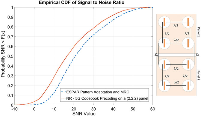
FIGURE 14. Performance comparison between the proposed ESPAR with pattern selection and an 8-element, 2-panel antenna using precoding codebooks from 5G-NR. The 8-element conventional antenna layout is also depicted.

The comparison is performed in terms of achieved SNR and the results are presented in Figure 14. The empirical CDF of the achieved SNR for 5,500 simulation runs is extracted, where it becomes clear that despite the fact that the proposed system has only two active elements, it clearly outperforms the performance of the 8-element conventional beamforming setup, offering an extra average gain that exceeds 3 dB for the 70% of the experiments. It should also be noted that pattern adaptation is performed as an open-loop scheme, so no additional communication overhead is introduced.

The specific result highlights the benefits of the use of parasitic arrays. The significant reduction of the required RF chains without any performance reduction indicates significant reduction of development and operational cost. The RF electronics are more expensive and consume significantly more power. Additionally, they increase the design and development complexity with the installation of multiple RF cables and electronics, that may be a quite difficult task, especially on UAVs. Design and development cost reduction by a factor of 4 can be considered (equivalent to the reduction of RF chains), since the parasitic antenna elements and the varactors do not introduce significant cost. It should also be noted that generally the ESPAR antennas can be quite more compact, since the inter element distance can be significantly decreased. For the specific example, both antennas occupy the same surface $\left(\lambda \times 4\lambda \right)$.

5 Conclusion

This paper investigates the performance gains provided by the use of reconfigurable pattern antenna technologies. The analysis is divided into two main sections: 1) the analytical evaluation and stochastic analysis of a low complexity antenna technique, that uses two RF chains and a set of available patterns to gradually and systematically adapt to the channel; 2) a system configuration that can implement such a system using electronically steerable antennas with the use of a dynamic adaptation/beamforming scheme. Initially, the system model and mode of operation is presented, where at each step one RF chain adapts to the radio channel, while the other remains constant in order to minimize transitions. The analytical results are presented for Nakagami-m fading distributions, that have been suitable for the description of UAV-ground links. Then stochastic analysis is performed using the Markov chain model to extract closed-expressions of the statistics of the received SNR.

An ESPAR configuration suitable for UAV communications with dipole antenna elements is introduced and evaluated. Two tilted ESPARs are then used in the GS in order to provide support to a very wide range of angles in the azimuth and elevation plane. Then, an implementation of the dynamic pattern adaptation scheme is presented. Central to its operation is the beamforming scheme that selects the pattern of the ESPAR that best-fits the channel. A four-step process is introduced in order to reduce complexity. The dynamic pattern adaptation scheme is evaluated with the use of channel models, where the benefits of the algorithm are highlighted in terms of spectral efficiency and coverage.

Data Availability Statement

The original contributions presented in the study are included in the article/Supplementary Material, further inquiries can be directed to the corresponding authors.

Author Contributions

KM was responsible for the implementation of the antenna pattern dynamic configuration. PB was responsible for the stochastic analysis framework. The main idea of the proposed approach and the overall paper supervision were the contributions of AK.

Funding

This research is co-financed by Greece and the European Union (European Social Fund- ESF) through the “Operational Programme Human Resources Development, Education and Lifelong Learning” in the context of the project “Reinforcement of Postdoctoral Researchers - 2nd Cycle” (MIS-5033021), implemented by the State Scholarships Foundation (IKY). The work is also co-funded by the University of Piraeus Research Center (UPRC).

Conflict of Interest

The authors declare that the research was conducted in the absence of any commercial or financial relationships that could be construed as a potential conflict of interest.

References

Abdi, A., Barger, H., and Kaveh, M. (2001). “A Simple Alternative to the Lognormal Model of Shadow Fading in Terrestrial and Satellite Channels,” in Proc. IEEE Vehicular Technology Conference, Atlantic City, NJ, October 7–11, 2001 (IEEE), 2058–2062. doi:10.1109/VTC.2001.957106

CrossRef Full Text | Google Scholar

Abramowitz, M., and Stegun, I. A. (1964). Handbook of Mathematical Functions: With Formulas, Graphs, and Mathematical Tables. Washington, DC: Courier Corporation.

Al-Hourani, A., Kandeepan, S., and Jamalipour, A. (2014). “Modeling Air-To-Ground Path Loss for Low Altitude Platforms in Urban Environments,” in 2014 IEEE Global Communications Conference (IEEE), 2898–2904.

Google Scholar

Amorim, R., Nguyen, H., Mogensen, P., Kovács, I. Z., Wigard, J., and Sorensen, T. B. (2017). Radio Channel Modeling for Uav Communication over Cellular Networks. IEEE Wireless Commun. Lett. 6, 514–517. doi:10.1109/lwc.2017.2710045

CrossRef Full Text | Google Scholar

Bai, D., Ghassemzadeh, S. S., Miller, R. R., and Tarokh, V. (2011). Beam Selection Gain versus Antenna Selection Gain. IEEE Trans. Inform. Theor. 57, 6603–6618. doi:10.1109/TIT.2011.2165814

CrossRef Full Text | Google Scholar

Balanis, C. A. (2016). Antenna Theory: Analysis and Design. 4th Edn. New York, NY: Wiley-Interscience.

Bithas, P. S., Nikolaidis, V., Kanatas, A. G., and Karagiannidis, G. K. (2020). Uav-to-ground Communications: Channel Modeling and Uav Selection. IEEE Trans. Commun. 68, 5135–5144. doi:10.1109/TCOMM.2020.2992040

CrossRef Full Text | Google Scholar

Bithas, P. S., and Rontogiannis, A. A. (2015). Mobile Communication Systems in the Presence of Fading/shadowing, Noise and Interference. IEEE Trans. Commun. 63, 724–737. doi:10.1109/tcomm.2015.2390625

CrossRef Full Text | Google Scholar

Bithas, P. S., Sagias, N. C., Mathiopoulos, P. T., Karagiannidis, G. K., and Rontogiannis, A. A. (2006). On the Performance Analysis of Digital Communications over Generalized-K Fading Channels. IEEE Commun. Lett. 10, 353–355. doi:10.1109/lcomm.2006.1633320

CrossRef Full Text | Google Scholar

Bucheli Garcia, J. C., Kamoun, M., and Sibille, A. (2020). Low-complexity Adaptive Spatial Processing of Espar Antenna Systems. IEEE Trans. Wireless Commun. 19, 3700–3711. doi:10.1109/TWC.2020.2975800

CrossRef Full Text | Google Scholar

Chandhar, P., Danev, D., and Larsson, E. G. (2018). Massive Mimo for Communications with Drone Swarms. IEEE Trans. Wireless Commun. 17, 1604–1629. doi:10.1109/TWC.2017.2782690

CrossRef Full Text | Google Scholar

Choi, Y.-S., and Lee, W.-S. (2020). “Reconfigurable Beam Switching Antenna with Horizontal Parasitic Element Reflector (Hper) for Uav Applications,” in 2020 IEEE International Symposium on Antennas and Propagation and North American Radio Science Meeting, Montreal, QC, Canada, July 5–10, 2020 (IEEE), 433–434. doi:10.1109/IEEECONF35879.2020.9330337

CrossRef Full Text | Google Scholar

Ding, X., Feng, L., Zou, Y., and Zhang, G. (2020). Deep Learning Aided Spectrum Prediction for Satellite Communication Systems. IEEE Trans. Veh. Technol. 69, 16314–16319. doi:10.1109/TVT.2020.3043837

CrossRef Full Text | Google Scholar

Geraci, G., Garcia-Rodriguez, A., Galati Giordano, L., López-Pérez, D., and Björnson, E. (2018). Understanding Uav Cellular Communications: From Existing Networks to Massive Mimo. IEEE Access 6, 67853–67865. doi:10.1109/ACCESS.2018.2876700

CrossRef Full Text | Google Scholar

Gradshteyn, I. S., and Ryzhik, I. M. (2000). Table of Integrals, Series, and Products. 6th Edn. New York, NY: Academic Press.

Jaeckel, S., Raschkowski, L., Börner, K., Thiele, L., Burkhardt, F., and Eberlein, E. (2016). Quasi Deterministic Radio Channel Generator User Manual and Documentation. Berlin: Fraunhofer Heinrich Hertz Institute Wireless Communications and Networks.

Jaeckel, S., Raschkowski, L., Börner, K., and Thiele, L. (2014). Quadriga: A 3-d Multi-Cell Channel Model with Time Evolution for Enabling Virtual Field Trials. IEEE Trans. Antennas Propagat. 62, 3242–3256. doi:10.1109/TAP.2014.2310220

CrossRef Full Text | Google Scholar

Jiang, C., and Zhu, X. (2020). Reinforcement Learning Based Capacity Management in Multi-Layer Satellite Networks. IEEE Trans. Wireless Commun. 19, 4685–4699. doi:10.1109/TWC.2020.2986114

CrossRef Full Text | Google Scholar

Kalis, A., Kanatas, A., and Papadias, C. (2008). A Novel Approach to MIMO Transmission Using a Single RF Front End. IEEE J. Select. Areas Commun. 26, 972–980. doi:10.1109/JSAC.2008.080813

CrossRef Full Text | Google Scholar

Kalis, A., Kanatas, A., and Papadias, B. (2014). Parasitic Antenna Arrays for Wireless MIMO Systems. New York, NY: Springer.

Karamalis, P., Skentos, N., and Kanatas, A. (2006). Adaptive Antenna Subarray Formation for Mimo Systems. IEEE Trans. Wireless Commun. 5, 2977–2982. doi:10.1109/TWC.2006.04532

CrossRef Full Text | Google Scholar

Khuwaja, A. A., Chen, Y., Zhao, N., Alouini, M.-S., and Dobbins, P. (2018). A Survey of Channel Modeling for UAV Communications. IEEE Commun. Surv. Tutorials 20, 2804–2821. doi:10.1109/comst.2018.2856587

CrossRef Full Text | Google Scholar

Kim, K.-S., Yoo, J.-S., Kim, J.-W., Kim, S., Yu, J.-W., and Lee, H. L. (2020). All-around Beam Switched Antenna with Dual Polarization for Drone Communications. IEEE Trans. Antennas Propagat. 68, 4930–4934. doi:10.1109/TAP.2019.2952006

CrossRef Full Text | Google Scholar

Michailidis, E. T., Nomikos, N., Trakadas, P., and Kanatas, A. G. (2020a). Three-dimensional Modeling of Mmwave Doubly Massive Mimo Aerial Fading Channels. IEEE Trans. Veh. Technol. 69, 1190–1202. doi:10.1109/TVT.2019.2956460

CrossRef Full Text | Google Scholar

Michailidis, E. T., Potirakis, S. M., and Kanatas, A. G. (2020b). Ai-inspired Non-terrestrial Networks for Iiot: Review on Enabling Technologies and Applications. IoT 1, 21–48. doi:10.3390/iot1010003

CrossRef Full Text | Google Scholar

Molisch, A. F., Win, M. Z., Yang-Seok Choi, Yang-Seok., and Winters, J. H. (2005). Capacity of Mimo Systems with Antenna Selection. IEEE Trans. Wireless Commun. 4, 1759–1772. doi:10.1109/TWC.2005.850307

CrossRef Full Text | Google Scholar

Ohira, T., and Gyoda, K. (2000). “Electronically Steerable Passive Array Radiator Antennas for Low-Cost Analog Adaptive Beamforming,” in International Conference on Phased Array Systems and Technology, 101–104. doi:10.1109/PAST.2000.858918

CrossRef Full Text | Google Scholar

Ramírez, T., and Mosquera, C. (2020). “Resource Management in the Multibeam Noma-Based Satellite Downlink,” in ICASSP 2020 - 2020 IEEE International Conference on Acoustics, Speech and Signal Processing (ICASSP), Barcelona, Spain, May 4–8, 2020 (IEEE), 8812–8816. doi:10.1109/ICASSP40776.2020.9054692

CrossRef Full Text | Google Scholar

Rinaldi, F., Määttänen, H.-L., Torsner, J., Pizzi, S., Andreev, S., Iera, A., et al. (2021). Broadcasting Services over 5g Nr Enabled Multi-Beam Non-terrestrial Networks. IEEE Trans. Broadcast. 67, 33–45. doi:10.1109/TBC.2020.2991312

CrossRef Full Text | Google Scholar

Simon, M. K., and Alouini, M.-S. (2005). Digital Communication over Fading Channels. 2nd Edn. New York, NY: Wiley.

Sun, C., Hirata, A., Ohira, T., and Karmakar, N. C. (2004). Fast Beamforming of Electronically Steerable Parasitic Array Radiator Antennas: Theory and Experiment. IEEE Trans. Antennas Propagat. 52, 1819–1832. doi:10.1109/TAP.2004.831314

CrossRef Full Text | Google Scholar

TR38.901, G. (2018). Tr 38.901 version 14.3.0 release 14 - study on channel model for frequencies from 0.5 to 100 ghz

Google Scholar

TS38.211, G. (2021). Ts 38.211 version 16.5.0 release 16 - 5g-nr physical channels and modulation

Google Scholar

TS38.214, G. (2020). Ts 138 214 v16.2.0 (2020-07) - 5g-nr physical layer procedures for data

Google Scholar

Vasileiou, P., Maliatsos, K., Thomatos, E., and Kanatas, A. (2013). Reconfigurable Orthonormal Basis Patterns Using Espar Antennas. IEEE Antennas Wireless Propagation Lett. 12, 448–451. doi:10.1109/LAWP.2013.2255254

CrossRef Full Text | Google Scholar

Wang, K., Zhang, R., Wu, L., Zhong, Z., He, L., Liu, J., et al. (2017). “Path Loss Measurement and Modeling for Low-Altitude Uav Access Channels,” in 2017 IEEE 86th Vehicular Technology Conference (VTC-Fall), Toronto, ON, Canada, September 24–27, 2017 (IEEE), 1–5. doi:10.1109/VTCFall.2017.8288385

CrossRef Full Text | Google Scholar

Wolfe, S., Begashaw, S., Liu, Y., and Dandekar, K. R. (2018). “Adaptive Link Optimization for 802.11 Uav Uplink Using a Reconfigurable Antenna,” in MILCOM 2018 - 2018 IEEE Military Communications Conference (MILCOM), Los Angeles, CA, October 29–31, 2018 (IEEE), 1–6. doi:10.1109/MILCOM.2018.8599696

CrossRef Full Text | Google Scholar

Yan, X., An, K., Liang, T., Zheng, G., Ding, Z., Chatzinotas, S., et al. (2019). The Application of Power-Domain Non-orthogonal Multiple Access in Satellite Communication Networks. IEEE Access 7, 63531–63539. doi:10.1109/ACCESS.2019.2917060

CrossRef Full Text | Google Scholar

Zhang, C., Zhang, W., Wang, W., Yang, L., and Zhang, W. (2019). Research Challenges and Opportunities of Uav Millimeter-Wave Communications. IEEE Wireless Commun. 26, 58–62. doi:10.1109/MWC.2018.1800214

CrossRef Full Text | Google Scholar

Zhao, J., Gao, F., Wu, Q., Jin, S., Wu, Y., and Jia, W. (2018). Beam Tracking for Uav Mounted Satcom On-The-Move with Massive Antenna Array. IEEE J. Selected Areas Commun. 36, 363–375. doi:10.1109/JSAC.2018.2804239

CrossRef Full Text | Google Scholar

Zhu, C., Mietzner, J., and Schober, R. (2010). On the Performance of Non-coherent Transmission Schemes with Equal-Gain Combining in Generalized K-Fading. IEEE Trans. wireless Commun. 9, 1337–1349.

CrossRef Full Text | Google Scholar