Isotropic and Non-Isotropic Signaling in Multivariate α-Stable Noise

1 Introduction

In many communication systems, additive Gaussian noise is the dominant form of signal corruption due to thermal fluctuations in the electronic devices comprising the receiver. Nevertheless, additive non-Gaussian noise has also been observed to play an important role in power line (Zimmermann and Dostert, 2002) and molecular communications (Farsad et al., 2015). Even in wireless communications, interference from uncoordinated transmitters, such as in the Internet of Things (IoT), has been suggested to admit non-Gaussian statistics (Clavier et al., 2021b). Another form of wireless communications where non-Gaussian noise arises is in underwater communications (Chitre et al., 2004).

A particularly important family of non-Gaussian noise models are impulsive, where the probability of large amplitude noise is significantly higher than predicted by corresponding Gaussian models; that is, impulsive noise is heavy-tailed. A key property of impulsive noise is that higher-order moments are often infinite or undefined, arising in Student’s t (Hall, 1966), generalized Gaussian (Dytso et al., 2018), and α-stable models (Middleton, 1977; Sousa, 1992; Ilow and Hatzinakos, 1998; Gulati et al., 2010; Pinto and Win, 2010).

Of all impulsive noise families, one of the most ubiquitous are the α-stable models. As a generalization of Gaussian models admitting the key property known as stability under convolution, these models arise via several mechanisms. The first mechanism, relevant for molecular communications, is via the distribution of the first hitting time of the standard Wiener process (Farsad et al., 2015). The second mechanism is via the generalized central limit theorem, which characterizes the behavior of partial sums of n independent and identically distributed random variables under the scaling $n^{-\frac{1}{\alpha }}$ (Mahmood et al., 2014).

The third mechanism to obtain α-stable models relevant for interference in wireless communication systems was first identified by Middleton (Middleton, 1977) and further clarified in (Sousa, 1992; Ilow and Hatzinakos, 1998). In particular, given uncoordinated transmitting devices located according to a homogeneous Poisson point process on the plane, the interference under power-law path loss converges almost surely to an α-stable random variable by identification with the LePage series (Samorodnitsky and Taqqu, 1994). This third mechanism has recently seen application in interference studies for the IoT (Egan et al., 2018). Indeed both theory and recent experimental data (Lauridsen et al., 2017) in the 868 MHz band, utilized by SigFox and LoRa devices, has indicated the presence of heavy-tailed interference which may be modeled via α-stable models (Clavier et al., 2021b).

Despite the utility of α-stable noise models in communications, the vast majority of work has focused on real-valued noise. In this setting, information capacity bounds have been derived in (de Freitas et al., 2017) and the structure of optimal input distributions characterized in (Fahs and Abou-Faycal, 2017). The design of symbol detection strategies and their performance has been addressed in (Niranjayan and Beaulieu, 2009; Ghannudi et al., 2010; Clavier et al., 2021a) and decoding algorithms developed in (Gu and Clavier, 2012; Mestrah et al., 2020). Noise parameter estimation algorithms have also been developed in (Kuruoglu, 2001) and power control strategies in (Freitas et al., 2018).

On the other hand, baseband signals in wireless communications are typically complex-valued for which few signal processing strategies and studies of performance analysis have been developed, with notable exceptions in (Gulati et al., 2010; Mahmood et al., 2014) for the narrowband case. The situation is further complicated when transmissions utilize orthogonal frequency division multiplexing (OFDM), where signals are transmitted over multiple subcarriers. In such cases, the noise forms a random vector and real-valued α-stable models are insufficient. Nevertheless, it has recently been shown that multivariate α-stable models can naturally arise from statistical analysis of interference in complex baseband signals over multiple subcarriers (Egan et al., 2018). However, little is known about performance limits or optimal signaling strategies in the presence of multivariate α-stable noise. In particular, the information capacity remains an open question in such channels, which is useful for selecting coding rates—via the noisy channel coding theorem—and in designing resource allocation strategies (Freitas et al., 2018).

In this paper, as a step towards resolving these open questions, we study the information capacity and signaling in multivariate symmetric α-stable noise channels with 1 < α < 2. We first return to the question of the information capacity in real-valued symmetric α-stable noise channels, where we establish new upper and lower bounds that are tighter and more general than those given in (de Freitas et al., 2017). In particular, bounds are also given for power-constrained inputs as well as fractional moment constraints. In the case of a power constraint, we establish that the information capacity is within a constant of the information capacity for the Gaussian noise channel and that Gaussian inputs yield this behavior.

We then turn to the case of multivariate symmetric α-stable noise. We show that there exists a unique optimal input achieving the information capacity and also derive a general upper bound, which is applicable to all multivariate symmetric α-stable noise channels subject to fractional moment and power constraints. We then derive a general lower bound applicable for fractional moment constraints with exponent r < α. In the case of sub-Gaussian α-stable models, we also obtain a lower bound on the information capacity subject to a power constraint.

Our bounds suggest, at least from an analytical point of view, that it is desirable to match the dependence structure of the input distribution to that of the noise. Indeed, our lower bounds are obtained with non-isotropic inputs, often matched to the dependence structure of the noise distribution. To study the performance of non-isotropic inputs, we consider communication in sub-Gaussian α-stable noise subject to a power constraint, and numerically study the behavior of the bounds. In this particular case, we observe that isotropic Gaussian inputs nearly achieve the capacity upper bound, suggesting that matching the input to the dependence structure of the noise is not always desirable.

1.1 Notation

Vectors are denoted by bold lowercase letters and random vectors by bold uppercase letters, respectively (e.g., x, X). We denote the distribution of a random vector X by P_X. If X, Y are two random vectors equal in distribution, then we write $\mathbf{X}\underset{\Vert }{d}\mathbf{Y}$.

Let $\mathbf{z}\in {\mathbb{R}}^d$, then ‖z‖_r, 1 ≤ r ≤ 2 is given by

$\Vert \mathbf{z}{\Vert }_r={\left(\sum _{i=1}^d|z_i{|}^r\right)}^{\frac{1}{r}}(1)$

and ‖·‖_r is called the r-norm on ${\mathbb{R}}^d$. For two vectors $\mathbf{a},\mathbf{b}\in {\mathbb{R}}^n$, a ⪰ b indicates that a_i ≥ b_i, i = 1, … , n.

Let $f:\mathbb{R}\to \mathbb{R}$ and $g:\mathbb{R}\to \mathbb{R}$. We use the Landau notation where f(x) = o(g(x)) if ${\lim }_{x\to \infty }\frac{f(x)}{g(x)}=0$ and f(x) = O(g(x)) if there exists C > 0 and $x_0\in \mathbb{R}$ such that f(x) ≤ Cg(x), ∀x ≥ x₀.

2 Problem Formulation

In this section, we detail the problem of characterizing the information capacity and optimal input distributions in multivariate symmetric α-stable noise channels (1 < α < 2). To this end, we first recall preliminary definitions and properties of scalar and multivariate α-stable models that will be used in the sequel. For further details, we refer the reader to (Samorodnitsky and Taqqu, 1994).

2.1 α-Stable Models

The probability density function of an α-stable random variable is described by four parameters: the exponent 0 < α ≤ 2; the scale parameter $\gamma \in {\mathbb{R}}_{+}$; the skew parameter β ∈ ( − 1, 1); and the shift parameter $\delta \in \mathbb{R}$. If X has an α-stable distribution, then we write X ∼ S_α(γ, β, δ). In the case β = δ = 0, X is said to be a symmetric α-stable random variable.

In general, α-stable random variables do not have closed-form probability density functions. Instead, they are more compactly represented by the characteristic function, given by (Samorodnitsky and Taqqu, 1994, Eq. 1.1.6)

$\begin{array}{ll}\hfill & \mathbb{E}[e^{i\theta X}]\hfill \\ \hfill & =\left\{\begin{array}{c}\exp \left\{-{\gamma }^{\alpha }|\theta {|}^{\alpha }\left(1-i\beta (\mathrm{sign}\theta )\tan \frac{\pi \alpha }{2}\right)+i\delta \theta \right\},\hfill \\ \alpha \ne 1\hfill \\ \exp \left\{-\gamma |\theta |\left(1+i\beta \frac{2}{\pi }(\mathrm{sign}\theta )\log |\theta |\right)+i\delta \theta \right\},\hfill \\ \alpha =1\hfill \end{array}\right.\hfill \end{array}(2)$

Observe that in the special case α = 2, the α-stable distribution is Gaussian. As such, the family of α-stable distribution generalize the family of Gaussian distributions. In fact, like Gaussian models, if X⁽¹⁾ and X⁽²⁾ are independent copies of an α-stable random variable X, then for a, b > 0, there exists constants $c>0,d\in \mathbb{R}$ such that

$a{X}^{(1)}+b{X}^{(2)}\underset{\Vert }{d}cX+d.(3)$

More precisely, the following property holds (Samorodnitsky and Taqqu, 1994).

Property 1 Suppose Z₁, Z₂ are independent with Z₁ ∼ S_α(γ₁, β₁, δ₁) and Z₂ ∼ S_α(γ₂, β₂, δ₂). Then, Z₁ + Z₂ ∼ S_α(γ, β, δ), where

$\begin{array}{ll}\hfill \gamma & ={({\gamma }_1^{\alpha }+{\gamma }_2^{\alpha })}^{\frac{1}{\alpha }},\hfill \\ \hfill \beta & =\frac{{\beta }_1{\gamma }_1^{\alpha }+{\beta }_2{\gamma }_2^{\alpha }}{{\gamma }_1^{\alpha }+{\gamma }_2^{\alpha }}\hfill \\ \hfill \delta & ={\delta }_1+{\delta }_2.\hfill \end{array}(4)$

When β = δ = 0 in Eq. 2, the resulting α-stable distribution is said to be symmetric. An important alternative characterization of symmetric α-stable random variables is via the LePage series.

Theorem 1 [Theorem 1.4.2 (Samorodnitsky and Taqqu, 1994)]. Suppose 0 < α < 2,${({\mathrm{\Gamma }}_i)}_{i=1}^{\infty }$ is a homogeneous Poisson point process with intensity 1, and ${(W_i)}_{i=1}^{\infty }$ are symmetric, independent and identically distributed random variables satisfying $\mathbb{E}[|W_i{|}^{\alpha }]<\infty$. Then,

$\sum _{i=1}^{\infty }{\mathrm{\Gamma }}_i^{-\frac{1}{\alpha }}{W}_i(5)$

converges almost surely to a random variable $X\sim S_{\alpha }({(C_{\alpha }^{-1}\mathbb{E}[|W_1{|}^{\alpha }])}^{1/\alpha },\mathrm{0,0})$, where

$C_{\alpha }=\left\{\begin{array}{cc}\frac{1-\alpha }{\mathrm{\Gamma }(2-\alpha )\cos (\pi \alpha /2)},\hfill & \alpha \ne 1\hfill \\ 2/\pi ,\hfill & \alpha =1.\hfill \end{array}\right.(6)$

In the multivariate setting, we consider random vectors X in ${\mathbb{R}}^d\sim d>1$. Analogously to the scalar case (d = 1), a random vector $\mathbf{X}\in {\mathbb{R}}^d$ is a symmetric α-stable random vector if for all a, b > 0 there exists c > 0 such that

$a{\mathbf{X}}^{(1)}+b{\mathbf{X}}^{(2)}\underset{\Vert }{d}c\mathbf{X},(7)$

where X⁽¹⁾ and X⁽²⁾ are independent copies of X.A sufficient condition for a random vector X in ${\mathbb{R}}^d$ to be a symmetric α-stable random vector is that all linear combinations of the elements of X are symmetric α-stable (Samorodnitsky and Taqqu, 1994). In general, d-dimensional symmetric α-stable random vectors can be represented via their characteristic function, given by (Samorodnitsky and Taqqu, 1994)

$\mathbb{E}[e^{i\mathit{\theta }\cdot \mathbf{X}}]=\exp \left(-{\int }_{{\mathbb{S}}^{d-1}}{\left|\sum _{k=1}^d{\theta }_k{s}_k\right|}^{\alpha }\mathrm{\Gamma }(d\mathbf{s})\right),(8)$

where Γ is the unique symmetric measure on the surface of the d-dimensional unit sphere.In the case that a d-dimensional α-stable random vector X is truly d-dimensional, there exists a joint probability density function p_X(⋅) on ${\mathbb{R}}^d$. Note that a simple necessary and sufficient condition for X to be truly d-dimensional is for the support of the spectral measure to span ${\mathbb{R}}^d$ (Byczkowski et al., 1993). This condition means that degenerate α-stable random vectors (e.g., when X_i = X_j for some i ≠ j, i, j ∈ {1, … , d}) are not considered.A key family of truly α-stable random vectors are the sub-Gaussian α-stable random vectors, defined as follows.

Definition 1 Any vector X satisfying $\mathbf{X}\underset{\Vert }{d}(A^{1/2}{G}_1,\dots ,A^{1/2}{G}_d)$, where

$A\sim S_{\alpha /2}({(\cos \pi \alpha /4)}^{2/\alpha },\mathrm{1,0}),(9)$

and $\mathbf{G}={[G_1,\dots ,G_d]}^T\sim \mathcal{N}(\mathbf{0},\mathrm{\Sigma })$ is called a sub-Gaussian α-stable random vector in ${\mathbb{R}}^d$ with underlying Gaussian vector G. IfΣ = σ²I with σ > 0, then X is said to be an isotropic sub-Gaussian α-stable random vector.

2.2 The Information Capacity Problem

Consider the memoryless, stationary, linear and point-to-point communication channel

$\mathbf{Y}=\mathbf{X}+\mathbf{N},(10)$

where N is a truly symmetric α-stable random vector with 1 < α < 2, admitting a multivariate probability density function p_N(⋅), with X and N independent. The random vector X is defined on¹$({\mathbb{R}}^d,\mathcal{B}({\mathbb{R}}^d))$ with probability measure μ_X lying in the set Λ_X (P, r), where

${\mathrm{\Lambda }}_{\mathbf{X}}(\mathbf{P},r)=\{{\mu }_{\mathbf{X}}:({\mathbb{E}}_{{\mu }_{\mathbf{X}}}[|X_1{|}^r],\dots ,\mathbb{E}[|X_d{|}^r])⪰\mathbf{P}\},(11)$

for a given $\mathbf{P}\in {\mathbb{R}}_{+}^d$ and 1 ≤ r ≤ 2. As such, the set Λ_X(P, r) corresponds to the set of inputs satisfying element-wise moment constraints. Note that by virtue of N admitting a probability density function, Y also admits a probability density function p_Y(⋅).

The main focus of this paper is to investigate the information capacity and corresponding optimal inputs for communication channels of the form Eq. 10. To this end, let $\mathcal{P}({\mathbb{R}}^d)$ be the set of probability measures on $({\mathbb{R}}^d,\mathcal{B}({\mathbb{R}}^d))$ equipped with the topology of weak convergence (Billingsley, 1999).

$C(\mathbf{P},r)=\underset{{\mu }_{\mathbf{X}}\in {\mathrm{\Lambda }}_{\mathbf{X}}(\mathbf{P},r)}{\text{sup}}I(\mathbf{X};\mathbf{Y})(12)$

where the mutual information I(X; Y) is given by

$I(\mathbf{X};\mathbf{Y})={\int }_{{\mathbb{R}}^d}{\int }_{{\mathbb{R}}^d}{p}_{\mathbf{N}}(\mathbf{y}-\mathbf{x})\log \frac{p_{\mathbf{N}}(\mathbf{y}-\mathbf{x})}{p_{\mathbf{Y}}(\mathbf{y})}\mathrm{d}\mathbf{y}{\mu }_{\mathbf{X}}(\mathrm{d}\mathbf{x}).(13)$

In the case an optimal input exists, it satisfies

${\mu }_{\mathbf{X}}^{*}\in \arg \underset{{\mu }_{\mathbf{X}}\in {\mathrm{\Lambda }}_{\mathbf{X}}(\mathbf{P},r)}{\max }I(\mathbf{X};\mathbf{Y}).(14)$

Note that, by a generalization of Shannon’s noisy channel coding theorem for vector non-Gaussian channels (Han, 2003), the information capacity may be interpreted as the maximum achievable rate with asymptotically zero average probability of error.

In the remainder of this paper, we address the following questions:

(i) What is the value of C(P, r) for varying P and r?

(ii) Does an optimal input ${\mu }_{\mathbf{X}}^{*}\in {\mathrm{\Lambda }}_{\mathbf{X}}(\mathbf{P},r)$ exist?

(iii) What is the structure of nearly optimal inputs?

In this work, we will allow μ_X to be non-isotropic; that is, for all d × d orthogonal matrices $\mathbf{O}\in \mathcal{O}(d)$, it does not hold that

$\mathbf{O}\mathbf{X}\underset{\Vert }{d}\mathbf{X},(15)$

where X has probability measure μ_X. In the following section, we begin with scalar channels—which have not previously been comprehensively studied—before considering more general vector channels in Section 4.

3 Scalar Channels

Before turning to multivariate α-stable noise channels, we first consider the scalar case. In particular, we first improve on the capacity bounds in (de Freitas et al., 2017) and in the process develop techniques that will be generalized to the multivariate setting in the sequel. To begin, we specialize the problem in Eq. 12 to the scalar case: a stationary and memoryless scalar additive symmetric α-stable noise channel is given by

$Y=X+N,(16)$

where the noise N is a symmetric α-stable random variable with scale parameter γ_N, admiting a probability density function p_N(⋅), with X and N independent. The input random variable X is required to satisfy the constraint

$\mathbb{E}[|X{|}^r]\le P,(17)$

where 1 ≤ r ≤ 2. In terms of the probability measure of X, the constraint can be written as

${\mathrm{\Lambda }}_X(P,r)=\{{\mu }_X\in \mathcal{P}(\mathbb{R}):{\mathbb{E}}_{{\mu }_X}[|X{|}^r]\le P\}.(18)$

In this case, the information capacity of the channel (16) is defined as

$C(P)=\underset{\mu \in {\mathrm{\Lambda }}_X(P,r)}{\text{sup}}I(X;Y)(19)$

It follows from (Fahs and Abou-Faycal, 2016) that an optimal solution of Eq. 19 exists and is unique. Indeed, the optimal input is known to be discrete (Fahs and Abou-Faycal, 2017).

3.1 Capacity Upper Bounds

In (de Freitas et al., 2017), an upper bound on C(P, r) was established when r = 1 and 1 < α < 2.

Theorem 2 Letλ > 0 and r = 1. For the channel (16), the capacity C(P, 1) in (19) is upper bounded by

$C(P,1)\le \log \left(\frac{2\mathrm{\Gamma }\left(\frac{1}{\alpha }\right)}{\lambda \gamma \alpha \pi }\right)+\lambda \left(\frac{2\gamma \mathrm{\Gamma }\left(1-\frac{1}{\alpha }\right)}{\pi }+P\right).(20)$

It was shown in (de Freitas et al., 2017) that this bound was tight for moderate values of P and appropriate values of λ, but quickly diverged. An asymptotic upper bound, that is, the upper bound is only guaranteed to hold as P → ∞, was established. In the following theorem, we establish an upper bound which holds for all 1 ≤ r ≤ 2 and p > 0.

Theorem 3 Let 1 ≤ r ≤ 2 and p > 0. For the channel (16), the capacity C(P, r) in (19) is upper bounded by

$\begin{array}{ll}\hfill C(P,r)& \le C_{UB}(P,r)\hfill \\ \hfill & =\log \left(2\left(P^{\frac{1}{r}}+\frac{2\mathrm{\Gamma }\left(1-\frac{1}{\alpha }\right)}{\pi }{\gamma }_N\right)e\right)-h(N).\hfill \end{array}(21)$

Proof. Note that under the constraint that $\mathbb{E}[|Y|]=c_Y,c_Y>0$, the entropy is maximized by the Laplace distribution (Cover and Thomas, 2006). This yields a bound of

$h(Y)\le \log (2c_{Y}e).(22)$

By the triangle inequality,

$\mathbb{E}[|Y|]\le \mathbb{E}[|X|]+\mathbb{E}[|N|].(23)$

We also have by (Zolotarev, 1957)

$\mathbb{E}[|N|]=\frac{2\mathrm{\Gamma }\left(1-\frac{1}{\alpha }\right)}{\pi }{\gamma }_N.(24)$

All that remains is to obtain $\mathbb{E}[|X{|}^r]$. By construction, $\mathbb{E}[|X{|}^r]\le P$. Using Hölder’s inequality then yields

$\mathbb{E}[|X|]\le {(\mathbb{E}[|X{|}^r])}^{\frac{1}{r}}=P^{\frac{1}{r}}.(25)$

Substituting Eqs 23–25 into Eq. 22 gives

$C(P)\le \log \left(2\left(P^{\frac{1}{r}}+\frac{2\mathrm{\Gamma }\left(1-\frac{1}{\alpha }\right)}{\pi }{\gamma }_N\right)e\right)-h(N),(26)$

as required.

3.2 Capacity Lower Bounds

We now turn to lower bounding C(P, r). We first consider the case where 1 ≤ r < α.

Theorem 4 Let 1 ≤ r < α. For the channel (16), the capacity C(P, r) in (19) is lower bounded by

$\begin{array}{ll}\hfill C(P,r)& \ge C_{LB}(P,r)\hfill \\ \hfill & =\frac{1}{\alpha }\log \left(1+\frac{P^{\frac{\alpha }{r}}}{{\gamma }_N^{\alpha }}{\left(\frac{\alpha \sqrt{\pi }\mathrm{\Gamma }\left(-\frac{r}{2}\right)}{2^{r+1}\mathrm{\Gamma }\left(\frac{r+1}{2}\right)\mathrm{\Gamma }\left(-\frac{r}{\alpha }\right)}\right)}^{\frac{1}{r}}\right).\hfill \end{array}(27)$

Proof. Let X ∼ S_α(γ_X, 0, 0) with ${\gamma }_X\in {\mathbb{R}}_{+}$. Consider the random variable U ∼ S_α(1, 0, 0). By the scaling and translation properties of α-stable random variables, we can write

$\begin{array}{l}\hfill X\underset{\Vert }{d}{\gamma }_{X}U\\ \hfill N\underset{\Vert }{d}{\gamma }_{N}U.\end{array}(28)$

By the stability property

$Y=X+N\sim S_{\alpha }\left({({\gamma }_X^{\alpha }+{\gamma }_N^{\alpha })}^{\frac{1}{\alpha }},\mathrm{0,0}\right)(29)$

and hence

$Y\underset{\Vert }{d}{\gamma }_{Y}U,(30)$

where ${\gamma }_Y={({\gamma }_X^{\alpha }+{\gamma }_N^{\alpha })}^{\frac{1}{\alpha }}$.We then have

$\begin{array}{ll}\hfill I(X;Y)& =h(Y)-h(Y|X)\hfill \\ \hfill & =h({\gamma }_{Y}U)-h({\gamma }_{N}U)\hfill \\ \hfill & =h(U)+\log ({\gamma }_Y)-h(U)-\log ({\gamma }_N)\hfill \\ \hfill & =\log \left(\frac{{({\gamma }_X^{\alpha }+{\gamma }_N^{\alpha })}^{\frac{1}{\alpha }}}{{\gamma }_N}\right)\hfill \\ \hfill & =\frac{1}{\alpha }\log \left(1+\frac{{\gamma }_X^{\alpha }}{{\gamma }_N^{\alpha }}\right).\hfill \end{array}(31)$

Using (Shao and Nikias, 1993, Theorem 4)

$\mathbb{E}[|X{|}^r]=\frac{2^{r+1}\mathrm{\Gamma }\left(\frac{r+1}{2}\right)\mathrm{\Gamma }\left(-\frac{r}{\alpha }\right)}{\alpha \sqrt{\pi }\mathrm{\Gamma }\left(\frac{-r}{2}\right)}{\gamma }_X^r.(32)$

and the constraint $\mathbb{E}[|X{|}^r]\le P$, it follows that

$C(P)\ge \frac{1}{\alpha }\log \left(1+\frac{P^{\frac{\alpha }{r}}}{{\gamma }_N^{\alpha }}{\left(\frac{\alpha \sqrt{\pi }\mathrm{\Gamma }\left(-\frac{r}{2}\right)}{2^{r+1}\mathrm{\Gamma }\left(\frac{r+1}{2}\right)\mathrm{\Gamma }\left(-\frac{r}{\alpha }\right)}\right)}^{\frac{1}{r}}\right).(33)$

Remark 1 When r = 1, Theorem 4 specializes to the lower bound in (de Freitas et al., 2017).

Since 1 ≤ r < α and α < 2, it follows that Theorem 4 does not apply in the important case where the input X is constrained to satisfy $\mathbb{E}[X^2]\le P$. In the following theorem, we establish a lower bound in this setting.

Theorem 5 Let r = 2. For the channel (16), the capacity C(P, 2) in (19) is lower bounded by

$\begin{array}{ll}\hfill C(P,2)& \ge C_{LB}(P,2)\hfill \\ \hfill & ={\int }_0^{\infty }\frac{1}{2}{p}_A(a)\log (2\pi e(P+a))\mathrm{d}a-h(N),\hfill \end{array}(34)$

where p_A(a) is the probability density function of a totally skewed α/2-stable random variable with scale parameter ${\cos }^{2/\alpha }(\frac{\pi }{4}\alpha )$.

Proof. Let $X\sim \mathcal{N}(0,P)$ and $G\sim \mathcal{N}(\mathrm{0,2}{\gamma }_N^2)$. Then,

$\begin{array}{ll}\hfill h(Y)& =h(X+N)\hfill \\ \hfill & =h(X+A^{1/2}G)\hfill \\ \hfill & \ge h(X+A^{1/2}G|A)\hfill \\ \hfill & =h(G_A|A),\hfill \end{array}(35)$

where $G_A\sim \mathcal{N}(0,P+A{\gamma }_N^2)$. Hence,

$h(Y)\ge {\int }_0^{\infty }\frac{1}{2}{p}_A(a)\log (2\pi e(P+2a{\gamma }_N^2))\mathrm{d}a.(36)$

As such,

$C(P)\ge {\int }_0^{\infty }\frac{1}{2}{p}_A(a)\log (2\pi e(P+2a{\gamma }_N^2))\mathrm{d}a-h(N),(37)$

as required.

A key question is whether the capacity bounds we have established so far are tight. To this end, we make the following observation.

Corollary 1 Let 1 ≤ r < α. For the channel (16), the capacity C(P, r) in (19) satisfies

$C(P,r)=\frac{1}{r}\log P+O(1),P\to \infty .(38)$

Proof. Observe that

$\begin{array}{ll}\hfill C_{LB}(P,r)& =\frac{1}{r}\log P+O(1),P\to \infty ,\hfill \\ \hfill C_{UB}(P,r)& =\frac{1}{r}\log P+O(1),P\to \infty .\hfill \end{array}(39)$

Since

$C_{LB}(P,r)\le C\le C_{UB}(P,r),(40)$

the corollary follows.

By the same argument, we also have the following corollary.

Corollary 2 Let r = 2. For the channel (16), the capacity C(P, 2) in (19) satisfies

$C(P,2)=\frac{1}{2}\log P+O(1),P\to \infty .(41)$

As a consequence, for sufficiently large values of P and r = 2, the rate achievable using a Gaussian input is within a constant of the capacity C(P, 2). A further observation, which will be useful in the sequel, is that matching the input distribution to the noise distribution yields a rate that forms a good approximation of the capacity. Finally, the capacity of symmetric α-stable noise channels is within a constant of the capacity for an additive Gaussian noise channel.

3.3 Numerical Results

In order to further verify the tightness of the upper bound in Theorem 3, we compare the bound with the numerical computation of the capacity via the Blahut-Arimoto algorithm (Blahut, 1972; Arimoto, 1972). Figure 1 plots the power against the information capacity for varying and α. The scale parameter is set as γ_N = 0.01. Observe that the upper bound and the numerical approximation are in good agreement. Note that the lower bound is obtained based on a Gaussian input is also in good agreement, despite the fact that the optimal input is discrete (Fahs and Abou-Faycal, 2017).

FIGURE 1

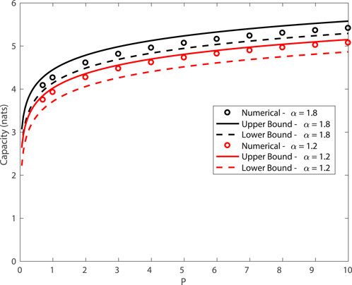
FIGURE 1. Capacity of symmetric α-stable noise channels subject to a power constraint P, with γ_N = 0.01.

Figure 2 plots the capacity upper bounds in Theorem 2 [from (de Freitas et al., 2017)] and our new upper bound in Theorem 3 in the case of the constraint $\mathbb{E}[|X|]\le P$ with γ_N = 0.01 and α = 1.8. The parameter λ required in the bound from Theorem 2 corresponds to λ = 1. Observe that for all plotted values of P, the new bound in Theorem 3 is below that of Theorem 2, implying that the new bound is tighter. Note that the improvement over the bound in (de Freitas et al., 2017) is already evident from the form of the bounds for large P, due to the fact that P dominates log  P.

FIGURE 2

FIGURE 2. Capacity of symmetric α-stable noise channels subject to the constraint $\mathbb{E}[|X|]\le P$, with γ_N = 0.01 and α = 1.8.

4 Vector Channels

In this section, we return to the general problem in Eq. 12 for vector channels with d > 1.

4.1 Existence and Uniqueness of Optimal Inputs

While existence and uniqueness of optimal inputs is well understood in the scalar case (Fahs and Abou-Faycal, 2016), it has not yet been established in the vector case. We prove this result in the following theorem by utilizing the theory of weak convergence (Billingsley, 1999).

Theorem 6 For the optimization problem in (12), there exists a unique input probability measure μ* corresponding to an input random vector X* on $({\mathbb{R}}^d,{\mathcal{B}}^d)$ such that C(P, r) = I(X*; Y).

Proof. The proof proceeds in three steps: (i) weak compactness of the constraint set Λ_X(P, r); (ii) weak continuity of I(X; Y) on Λ_X(P, r), yielding existence of ${\mu }_{\mathbf{X}}^{*}$; and (iii) uniqueness of ${\mu }_{\mathbf{X}}^{*}$.

(i) For any ϵ > 0, there exists ${\mathbf{a}}_{ϵ}={[a_{1,ϵ},\dots ,a_{d,ϵ}]}^T\succ 0$ such that for all μ ∈ Λ_X(P, r)

$\mathrm{Pr}\left(|X_1{|}^r>a_{1,ϵ},\dots ,|X_d{|}^r>a_{d,ϵ}\right)<ϵ.(42)$

The inequality in Eq. 42 holds as a consequence of the generalized Markov inequality in (Marshall, 1984, Example 2.3). In more detail,

$\begin{array}{ll}\hfill \mathrm{Pr}\left(|X_1{|}^r>a_{1,ϵ},\dots ,|X_d{|}^r>a_{d,ϵ}\right)& \le \underset{i=1,\dots ,d}{\min }\frac{\mathbb{E}[|X_i{|}^r]}{a_{i,ϵ}}\hfill \\ \hfill & \le \underset{i=1,\dots ,d}{\min }\frac{c_i}{a_{i,ϵ}}<ϵ.\hfill \end{array}(43)$

Now, choose ${\mathcal{K}}_{ϵ}=[-a_{1,ϵ},a_{1,ϵ}]\times \cdots \times [-a_{d,ϵ},a_{d,ϵ}]$. Then, ${\mathcal{K}}_{ϵ}$ is compact subset of ${\mathbb{R}}^d$ and $\mu ({\mathcal{K}}_{ϵ})\ge 1-ϵ$ for all μ ∈ Λ_X(P, r). Hence, Λ_X(P, r) is tight.To establish closure, we apply a variation of the Portmanteau theorem (Billingsley, 1999). Let ${\{{\mu }_n\}}_{n=1}^{\infty }$ be a weakly convergent sequence in Λ_X(P, r) with limit μ₀. By a consequence of the Portmanteau theorem, it follows that

$\begin{array}{ll}\hfill & {\left[{\mathbb{E}}_{{\mu }_0}[|X_1{|}^r],\dots ,\mathbb{E}[|X_d{|}^r]\right]}^T\hfill \\ \hfill & ={\left[\int |x_1{|}^{r}d{\mu }_0(\mathbf{x}),\dots ,\int |x_d{|}^{r}d{\mu }_0(\mathbf{x})\right]}^T\hfill \\ \hfill & ⪯{\left[\underset{n\to \infty }{\mathrm{lim\; inf}}\int |x_1{|}^{r}d{\mu }_n(\mathbf{x}),\dots ,\underset{n\to \infty }{\mathrm{lim\; inf}}\int |x_d{|}^{r}d{\mu }_n(\mathbf{x})\right]}^T\hfill \\ \hfill & ⪯\mathbf{P}.\hfill \end{array}(44)$

Hence, μ₀ ∈ Λ_X(P, r). Since the choice of sequence is arbitrary, it follows that Λ_X(P, r) is closed in the topology of weak convergence. Since Λ_X(P, r) is tight and closed in the topology of weak convergence, it then follows by Prokhorov’s theorem (Billingsley, 1999) that Λ_X(P, r) is compact.

(ii) The second step is to establish that I(X; Y) is weakly continuous on Λ_X(P, r). In particular, we need to show that for any weakly convergent sequence of probability measures ${({\mu }_n)}_{n=1}^{\infty }$ with limit μ₀

$\underset{n\to \infty }{\lim }-\int p_{{\mathbf{Y}}_n}(\mathbf{y})\log p_{{\mathbf{Y}}_n}(\mathbf{y})d\mathbf{y}=-\int p_{{\mathbf{Y}}_0}(\mathbf{y})\log p_{{\mathbf{Y}}_0}(\mathbf{y})d\mathbf{y},(45)$

where Y_n is the output corresponding to an input X_n with probability measure μ_n. Note that Y_n = X_n + N admits a probability density function since N is truly d-dimensional.Observe that if the limit and the integral in Eq. 45 can be swapped, the result follows from the definition of weak convergence if the probability density function of N, p_N, is bounded and continuous. Note that this is indeed the case since the characteristic function of N, ${\mathrm{\Phi }}_{\mathbf{N}}(\mathbf{t})=\mathbb{E}[e^{i\mathbf{t}\cdot \mathbf{N}}]$ is integrable when N is truly d-dimensional.To complete the proof, we must justify swapping of the limit and integral in Eq. 45. Let 1 < s < α. We need to establish that for all n ≥ 0 and any δ > 0, there exists R(δ) > 0 such that

$\left|{\int }_{\Vert \mathbf{y}{\Vert }_s>R(\delta )}{p}_{{\mathbf{Y}}_n}(\mathbf{y})\log p_{{\mathbf{Y}}_n}(\mathbf{y})d\mathbf{y}\right|<\delta .(46)$

To proceed, let

$q(\mathbf{y})=\frac{1}{{\pi }^d}\frac{1}{{\prod }_{i=1}^d(1+y_i^2)},\mathbf{y}\in {\mathbb{R}}^d.(47)$

which is a Cauchy density on ${\mathbb{R}}^d$. Observe that

$\begin{array}{ll}\hfill & -{\int }_{\Vert \mathbf{y}{\Vert }_s>R(\delta )}{p}_{{\mathbf{Y}}_n}(\mathbf{y})\log p_{{\mathbf{Y}}_n}(\mathbf{y})d\mathbf{y}\hfill \\ \hfill & =-{\int }_{\Vert \mathbf{y}{\Vert }_s>R(\delta )}{p}_{{\mathbf{Y}}_n}(\mathbf{y})\log q(\mathbf{y})d\mathbf{y}\hfill \\ \hfill & -{\int }_{\Vert \mathbf{y}{\Vert }_s>R(\delta )}{p}_{{\mathbf{Y}}_n}(\mathbf{y})\log \frac{p_{{\mathbf{Y}}_n}(\mathbf{y})}{q(\mathbf{y})}d\mathbf{y}\hfill \\ \hfill & \le {\int }_{\Vert \mathbf{y}{\Vert }_s>R(\delta )}{p}_{{\mathbf{Y}}_n}(\mathbf{y})\left(\log {\pi }^d+\log \prod _{i=1}^d(1+y_i^2)\right)d\mathbf{y}\hfill \\ \hfill & +\frac{1}{e}{\int }_{\Vert \mathbf{y}{\Vert }_s>R(\delta )}q(\mathbf{y})d\mathbf{y},\hfill \end{array}(48)$

where the last term follows from the fact that $a\log a\ge -\frac{1}{e},a>0$.Note that by the Markov inequality,

$\begin{array}{ll}\hfill {\int }_{\Vert \mathbf{y}{\Vert }_s>R(\delta )}\log {\pi }^d{p}_{{\mathbf{Y}}_n}(\mathbf{y})d\mathbf{y}& \le d\log \pi \frac{\mathbb{E}[\Vert \mathbf{Y}{\Vert }_s]}{R(\delta )}\hfill \\ \hfill & \le d\log \pi \frac{L}{R(\delta )},\hfill \end{array}(49)$

which tends to zero as R(δ) → ∞. Here, L < ∞ since by the Jensen and Hölder inequalities

$\begin{array}{ll}\hfill \mathbb{E}[\Vert \mathbf{X}{\Vert }_s]=\mathbb{E}\left[{\left(\sum _{i=1}^d|X_i{|}^s\right)}^{1/s}\right]& \le {\left(\mathbb{E}\left[\sum _{i=1}^d|X_i{|}^s\right]\right)}^{1/s}\hfill \\ \hfill & \le {\left(\sum _{i=1}^d{\left(\mathbb{E}\left[|X_i{|}^r\right]\right)}^{s/r}\right)}^{1/s}\hfill \end{array}(50)$

which implies

$\mathbb{E}[\Vert \mathbf{Y}{\Vert }_s]\le \mathbb{E}[\Vert \mathbf{X}{\Vert }_s]+\mathbb{E}[\Vert \mathbf{N}{\Vert }_s]\le {\left(\sum _{i=1}^d{\left(\mathbb{E}\left[|X_i{|}^r\right]\right)}^{s/r}\right)}^{1/s}+\mathbb{E}[\Vert \mathbf{N}{\Vert }_s]<L<\infty ,(51)$

since the probability measure μ corresponding to X lies in Λ_X(P, r). Similarly,

$\begin{array}{ll}\hfill & \frac{1}{e}{\int }_{\Vert \mathbf{y}{\Vert }_s>R(\delta )}q(\mathbf{y})d\mathbf{y}\hfill \\ \hfill & \le \frac{1}{eR(\delta )}{\mathbb{E}}_q[\Vert \mathbf{Y}{\Vert }_s],\hfill \end{array}(52)$

which tends to zero as R(δ) → ∞.Moreover,

$\begin{array}{ll}\hfill & {\int }_{\Vert \mathbf{y}{\Vert }_s>R(\delta )}{p}_{{\mathbf{Y}}_n}(\mathbf{y})\log \prod _{i=1}^d(1+y_i^2)d\mathbf{y}\hfill \\ \hfill & \le 2{\int }_{\Vert \mathbf{y}{\Vert }_s>R(\delta )}{p}_{{\mathbf{Y}}_n}(\mathbf{y})\log \prod _{i=1}^d(1+|y_i|)d\mathbf{y}\hfill \\ \hfill & \le 2\underset{\Vert \mathbf{y}{\Vert }_s>R(\delta )}{\sup }\left\{\frac{\log {\prod }_{i=1}^d(1+|y_i|)}{\Vert \mathbf{y}{\Vert }_s}\right\}{\int }_{\Vert \mathbf{y}{\Vert }_s>R(\delta )}\Vert \mathbf{y}{\Vert }_s{p}_{{\mathbf{Y}}_n}(\mathbf{y})d\mathbf{y}.\hfill \end{array}(53)$

Note that

$\frac{\log {\prod }_{i=1}^d(1+|y_i|)}{\Vert \mathbf{y}{\Vert }_s}\le \frac{{\sum }_{i=1}^d|y_i|}{\Vert \mathbf{y}{\Vert }_s}\le 1,(54)$

by Hölder’s inequality. As such, Eq. 53 is finite and tends to zero as R(δ) → ∞.After an application of the dominated convergence theorem, for any δ > 0

$\begin{array}{ll}\hfill & \underset{n\to \infty }{\lim }-{\int }_{\Vert \mathbf{y}{\Vert }_r\le R(\delta )}{p}_{{\mathbf{Y}}_n}(\mathbf{y})\log p_{{\mathbf{Y}}_n}(\mathbf{y})d\mathbf{y}\hfill \\ \hfill & =-{\int }_{\Vert \mathbf{y}{\Vert }_r\le R(\delta )}{p}_{{\mathbf{Y}}_0}(\mathbf{y})\log p_{{\mathbf{Y}}_0}(\mathbf{y})d\mathbf{y}.\hfill \end{array}(55)$

Since the identities in Eqs 49, 52, 53, 55 hold for all δ > 0, weak continuity of I(X; Y) follows by taking δ → 0 (and hence R(δ) → ∞). The existence part of Theorem 6 then holds by applying the extreme value theorem.

(iii) The uniqueness of the optimal input follows from the fact that the entropy h(Y) is a strictly concave function of the distribution P_Y. By the fact that the characteristic function of N is strictly positive, P_Y is a one-to-one function of the distribution P_X. Hence, h(Y) is a strictly concave function of P_X. As the mutual information can be written as

$I(\mathbf{X};\mathbf{Y})=h(\mathbf{Y})-h(\mathbf{N})(56)$

it follows that I(X; Y) is a strictly concave function of P_X since h(N) does not depend on P_X. Since this holds for any input lying in Λ(P, r), it then follows that the optimal input probability measure ${\mu }_{\mathbf{X}}^{*}$ is unique.

4.2 Capacity Upper Bound

We now obtain a general upper bound on the capacity in multivariate α-stable noise, which holds for constraints with 1 ≤ r ≤ 2.

Theorem 7 Let 1 < α < 2, 1 ≤ r ≤ 2,P⪰0 and ${\gamma }_{N_i}$ be the scale parameter for the ith element of N. The capacity C(P, r) in (12) is upper bounded by

$\begin{array}{ll}\hfill C(\mathbf{P},r)& \le C_{UB}(\mathbf{P},r)\hfill \\ \hfill & =\sum _{i=1}^d\log \left(2\left(P_i^{\frac{1}{r}}+\frac{2\mathrm{\Gamma }\left(1-\frac{1}{\alpha }\right)}{\pi }{\gamma }_{N_i}\right)e\right)-h(\mathbf{N}).\hfill \end{array}(57)$

Proof. Recall that

$h(\mathbf{Y})\le \sum _{i=1}^{d}h(Y_i).(58)$

For each term h(Y_i), the same argument as Theorem 3 yields

$h(Y_i)\le \log \left(2\left(P_i^{\frac{1}{r}}+\frac{2\mathrm{\Gamma }\left(1-\frac{1}{\alpha }\right)}{\pi }{\gamma }_{N_i}\right)e\right).(59)$

The result then follows since for all X with probability measure μ_X ∈ Λ(P, r),

$I(\mathbf{X};\mathbf{Y})\le \sum _{i=1}^{d}h(Y_i)-h(\mathbf{N}).(60)$

As for the scalar case, the term h(N) is not available in closed-form and must be numerically evaluated. In the numerical study in Section 4.4, h(N) will be estimated via nearest neighbor methods.

4.3 Capacity Lower Bounds

We now generalize the results in Section 3.2 to the case of vector channels. As for scalar channels, we consider the two cases: 1 ≤ r < α; and r = 2.

Theorem 8 Let 1 < α < 2, 1 ≤ r < α and P⪰0. The capacity C(P, r) in (12) is lower bounded by

$\begin{array}{ll}\hfill C(\mathbf{P},r)& \ge C_{LB}(\mathbf{P},r)\hfill \\ \hfill & =\frac{1}{\alpha }\sum _{i=1}^d\log \left(1+{\gamma }_{X_i}^{\alpha }\right),\hfill \end{array}(61)$

where

${\gamma }_{X_i}={\left(\frac{P_i\alpha \sqrt{\pi }\mathrm{\Gamma }\left(-\frac{r}{2}\right)}{2^{r+1}\mathrm{\Gamma }\left(\frac{r+1}{2}\right)\mathrm{\Gamma }\left(-\frac{r}{\alpha }\right){\gamma }_{N_i}^r}\right)}^{\frac{1}{r}}.$(62)

Proof. Let

$\begin{array}{ll}\hfill \mathbf{A}& =\mathrm{diag}({\gamma }_{X_1},\dots ,{\gamma }_{X_d})\hfill \\ \hfill {\mathbf{A}}^{\alpha }& =\mathrm{diag}({\gamma }_{X_1}^{\alpha },\dots ,{\gamma }_{X_d}^{\alpha })\hfill \end{array}(63)$

and set $\mathbf{X}\stackrel{d}{=}\mathbf{A}\mathbf{N}$. We then have

$\begin{array}{ll}\hfill I(\mathbf{X};\mathbf{Y})& =h(\mathbf{Y})-h(\mathbf{N})\hfill \\ \hfill & =h(\mathbf{X}+\mathbf{N})-h(\mathbf{N})\hfill \\ \hfill & =h\left({({\mathbf{A}}^{\alpha }+\mathbf{I})}^{\frac{1}{\alpha }}\mathbf{N}\right)-h(\mathbf{N})\hfill \\ \hfill & =\log \det {({\mathbf{A}}^{\alpha }+\mathbf{I})}^{\frac{1}{\alpha }}+h(\mathbf{N})-h(\mathbf{N})\hfill \\ \hfill & =\frac{1}{\alpha }\sum _{i=1}^d\log (1+{\gamma }_{X_i}^{\alpha }).\hfill \end{array}(64)$

In order to ensure that μ_X ∈ Λ_X(P, r), we recall (Shao and Nikias, 1993, Theorem 4)

$\begin{array}{ll}\hfill \mathbb{E}[|X_i{|}^r]& =\mathbb{E}[|{\gamma }_{X_i}{N}_i{|}^r]\hfill \\ \hfill & ={\gamma }_{X_i}^r\frac{2^{r+1}\mathrm{\Gamma }\left(\frac{r+1}{2}\right)\mathrm{\Gamma }\left(-\frac{r}{\alpha }\right)}{\alpha \sqrt{\pi }\mathrm{\Gamma }\left(\frac{-r}{2}\right)}{\gamma }_{N_i}^r\le P_i.\hfill \end{array}(65)$

It then follows that

${\gamma }_{X_i}={\left(\frac{P_i\alpha \sqrt{\pi }\mathrm{\Gamma }\left(-\frac{r}{2}\right)}{2^{r+1}\mathrm{\Gamma }\left(\frac{r+1}{2}\right)\mathrm{\Gamma }\left(-\frac{r}{\alpha }\right){\gamma }_{N_i}^r}\right)}^{\frac{1}{r}},(66)$

as required.

Theorem 9 Let 1 < α < 2, r = 2, and P⪰0 For the channel (10) with N sub-Gaussian α-stable with underlying random vector $\mathbf{G}\sim \mathcal{N}(0,\mathrm{\Sigma })$, the capacity C(P, 2) in (12) is lower bounded by

$\begin{array}{ll}\hfill C(\mathbf{P},2)& \ge C_{LB}(\mathbf{P},2)\hfill \\ \hfill & =\max \left\{0,{\int }_0^{\infty }\frac{1}{2}{p}_A(a)\log \det (2\pi e({\mathrm{\Sigma }}_{\mathbf{X}}+a\mathrm{\Sigma }))\mathrm{d}a-h(\mathbf{N})\right\},\hfill \end{array}(67)$

where Σ_X is any positive definite matrix with diagonal elements

${\mathrm{\Sigma }}_{\mathbf{X},ii}=P_i,i=1,\dots ,d(68)$

and $A\sim S_{\alpha /2}({\cos }^{2/\alpha }(\frac{\pi }{4}\alpha ),\mathrm{1,0})$.

Proof. Let $X\sim \mathcal{N}(0,{\mathrm{\Sigma }}_{\mathbf{X}})$ and $G\sim \mathcal{N}(0,\mathrm{\Sigma })$. Then,

$\begin{array}{ll}\hfill h(\mathbf{Y})& =h(\mathbf{X}+\mathbf{N})\hfill \\ \hfill & =h(\mathbf{X}+A^{1/2}\mathbf{G})\hfill \\ \hfill & \ge h(\mathbf{X}+A^{1/2}\mathbf{G}|A)\hfill \\ \hfill & =h({\mathbf{G}}_A|A),\hfill \end{array}(69)$

where ${\mathbf{G}}_A\sim \mathcal{N}(0,{\mathrm{\Sigma }}_{\mathbf{X}}+A\mathrm{\Sigma })$. Hence,

$h(\mathbf{Y})\ge {\int }_0^{\infty }\frac{1}{2}{p}_A(a)\log \det (2\pi e({\mathrm{\Sigma }}_{\mathbf{X}}+a\mathrm{\Sigma }))\mathrm{d}a.(70)$

In order to satisfy the power constraints, we require

${\mathrm{\Sigma }}_{\mathbf{X},ii}\le P_i,i=1,\dots ,d,(71)$

which yields the desired result.

4.4 Numerical Results

In this section, we study the behavior of the bounds in the case of two-dimensional sub-Gaussian α-stable noise, where inputs are subject to a power constraint.

Figure 3 plots the capacity bounds in the previous section for varying values of P in the presence of sub-Gaussian α-stable noise, with α = 1.2 and

$\mathrm{\Sigma }=2\cdot 0.01^2\cdot \left(\begin{array}{cc}\hfill 1\hfill & \hfill 0.7\hfill \\ \hfill 0.7\hfill & \hfill 1\hfill \end{array}\right).(72)$

In order to compute the entropy h(N), the 1-nearest neighbor method (Berrett et al., 2019) was used. Observe there is roughly a gap of approximately one nat between the upper bound in Theorem 7 and the lower bound in Theorem 9 with Σ_X chosen to proportional to Σ.

FIGURE 3

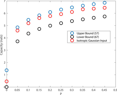
FIGURE 3. Capacity bounds for two-dimensional sub-Gaussian α-stable noise channels subject to a power constraint P, with Σ given in Eq. 72 and α = 1.2.

The third curve in red corresponds to the case of a two-dimensional isotropic Gaussian input where each component has variance P. Observe that the mutual information obtained with this input is close to the upper bound. This suggests that for sub-Gaussian α-stable noise channels, Gaussian inputs perform well and, moreover, independent components are desirable. This can be understood by an inspection of Theorem 9, where choosing Σ_X to be diagonal maximizes the determinant when Σ = 0.

Figure 4 plots the capacity bounds in the previous section subject to a power constraint p = 0.01 for varying values of ρ in the presence of sub-Gaussian α-stable noise, with α = 1.2 and

$\mathrm{\Sigma }=2\cdot 0.01^2\cdot \left(\begin{array}{cc}\hfill 1\hfill & \hfill \rho \hfill \\ \hfill \rho \hfill & \hfill 1\hfill \end{array}\right).(73)$

The results are consistent with Figure 3, with the isotropic Gaussian input performing well for all values of ρ. We also observe that the curves also increase for sufficient large values of ρ, suggesting that increasing the dependence can lead to performance improvements. This is relevant for communication systems, such as in (Zheng et al., 2019, 2020), where noise is dominated by interference, which may be modified via changes to access policies.

FIGURE 4

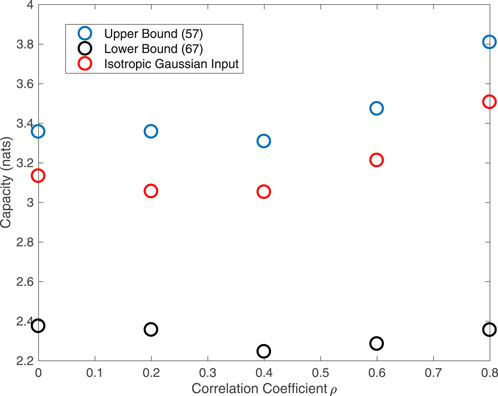
FIGURE 4. Capacity bounds for two-dimensional sub-Gaussian α-stable noise channels for varying noise dependence ρ subject to a power constraint p = 0.01, with Σ given in Eq. 73 and α = 1.2.

5 Conclusion

Multivariate α-stable models have been suggested to capture the heavy-tailed nature of interference in OFDM-based wireless communication systems. In this paper, we studied the capacity of fractional moment and power constrained signaling in the presence of such noise. By considering non-isotropic inputs, we obtained upper and lower bounds, which provide insights into the behavior of the capacity and its relation to Gaussian noise models. Via a numerical study in two-dimensional channels with sub-Gaussian α-stable noise, we compared the performance of isotropic and non-isotropic Gaussian inputs. This suggests, at least for this special case, isotropic Gaussian inputs remain a desirable choice.

Data Availability Statement

The original contributions presented in the study are included in the article/supplementary material, further inquiries can be directed to the corresponding author.

Author Contributions

ME formulated the problem, carried out the mathematical analysis and numerical study, and wrote the paper.

Funding

This work has been (partly) funded by the French National Agency for Research (ANR) under grant ANR-16-CE25-0001-ARBURST.

Conflict of Interest

The author declares that the research was conducted in the absence of any commercial or financial relationships that could be construed as a potential conflict of interest.

Publisher’s Note

All claims expressed in this article are solely those of the authors and do not necessarily represent those of their affiliated organizations, or those of the publisher, the editors and the reviewers. Any product that may be evaluated in this article, or claim that may be made by its manufacturer, is not guaranteed or endorsed by the publisher.

Acknowledgments

We would like to acknowledge useful discussions with L. Clavier, G. W. Peters, N. Azzaoui, and J.-M. Gorce.

Footnotes

¹The notation $\mathcal{B}({\mathbb{R}}^d)$ denotes the Borel σ-algebra on ${\mathbb{R}}^d$.

References

Arimoto, S. (1972). An Algorithm for Computing the Capacity of Arbitrary Discrete Memoryless Channels. IEEE Trans. Inform. Theor. 18, 14–20. doi:10.1109/tit.1972.1054753

CrossRef Full Text | Google Scholar

Berrett, T., Samworth, R., and Yuan, M. (2019). Efficient Multivariate Entropy Estimation via K-Nearest Neighbour Distances. Ann. Stat. 47, 288–318. doi:10.1214/18-aos1688

CrossRef Full Text | Google Scholar

Billingsley, P. (1999). Convergence of Probability Measures. John Wiley & Sons.

Google Scholar

Blahut, R. (1972). Computation of Channel Capacity and Rate-Distortion Functions. IEEE Trans. Inform. Theor. 18, 460–473. doi:10.1109/tit.1972.1054855

CrossRef Full Text | Google Scholar

Byczkowski, T., Nolan, J. P., and Rajput, B. (1993). Approximation of Multidimensional Stable Densities. J. Multivariate Anal. 46, 13–31. doi:10.1006/jmva.1993.1044

CrossRef Full Text | Google Scholar

Chitre, M., Potter, J., and Heng, O. (2004). “Underwater Acoustic Channel Characterisation for Medium-Range Shallow Water Communications,” in MTS/IEEE Techno-Ocean’04 (IEEE).

Google Scholar

Clavier, L., Pedersen, T., Larrad, I., Lauridsen, M., and Egan, M. (2021b). Experimental Evidence for Heavy Tailed Interference in the IoT. IEEE Commun. Lett. 25, 692–695. doi:10.1109/lcomm.2020.3034430

CrossRef Full Text | Google Scholar

Clavier, L., Peters, G., Septier, F., and Nevat, I. (2021a). Impulsive Noise Modeling and Robust Receiver Design. EURASIP J. Wireless Commun. Networking 13, 1. doi:10.1186/s13638-020-01868-1

CrossRef Full Text | Google Scholar

Cover, T., and Thomas, J. (2006). Elements of Information Theory. Second Edition. Hoboken, NJ: John Wiley & Sons.

Google Scholar

de Freitas, M. L., Egan, M., Clavier, L., Goupil, A., Peters, G. W., and Azzaoui, N. (2017). Capacity Bounds for Additive Symmetric $\alpha $ -Stable Noise Channels. IEEE Trans. Inform. Theor. 63, 5115–5123. doi:10.1109/tit.2017.2676104

CrossRef Full Text | Google Scholar

Dytso, A., Bustin, R., Vincent Poor, H., and Shamai, S. (2018). Analytical Properties of Generalized Gaussian Distributions. J. Stat. Distributions Appl. 5, 1–40. doi:10.1186/s40488-018-0088-5

CrossRef Full Text | Google Scholar

Egan, M., Clavier, L., Zheng, C., de Freitas, M., and Gorce, J.-M. (2018). Dynamic Interference for Uplink SCMA in Large-Scale Wireless Networks without Coordination. EURASIP J. Wireless Commun. Networking 213, 1. doi:10.1186/s13638-018-1225-z

CrossRef Full Text | Google Scholar

Egan, M. (2019). “On Capacity Sensitivity in Additive Vector Symmetric α-stable Noise Channels,” in Proc. IEEE Wireless Communications and Networking Conference Workshop (WCNCW) (IEEE). doi:10.1109/wcncw.2019.8902901

CrossRef Full Text | Google Scholar

Fahs, J., and Abou-Faycal, I. (2017). On Properties of the Support of Capacity-Achieving Distributions for Additive Noise Channel Models with Input Cost Constraints. IEEE Trans. Inf. Theor. 64, 1178–1198. doi:10.1109/TIT.2017.2771815

CrossRef Full Text | Google Scholar

Fahs, J., and Abou-Faycal, I. (2016). On the Finiteness of the Capacity of Continuous Channels. IEEE Trans. Commun. 64, 166–173. doi:10.1109/tcomm.2015.2503403

CrossRef Full Text | Google Scholar

Farsad, N., Guo, W., Chae, C.-B., and Eckford, A. (2015). “Stable Distributions as Noise Models for Molecular Communication,” in Proc. IEEE Global Communications Conference (IEEE). doi:10.1109/glocom.2015.7417583

CrossRef Full Text | Google Scholar

Freitas, M., Egan, M., Clavier, L., Savard, A., and Gorce, J.-M. (2018). “Power Control in Parallel Symmetric α-stable Noise Channels,” in IEEE International Workshop on Signal Processing Advances in Wireless Communications (SPAWC) (IEEE).

Google Scholar

Ghannudi, H. E., Clavier, L., Azzaoui, N., Septier, F., and Rolland, P.-a. (2010). α-Stable Interference Modeling and Cauchy Receiver for an IR-UWB Ad Hoc Network. IEEE Trans. Commun. 58, 1748–1757. doi:10.1109/tcomm.2010.06.090074

CrossRef Full Text | Google Scholar

Gu, W., and Clavier, L. (2012). Decoding Metric Study for Turbo Codes in Very Impulsive Environment. IEEE Commun. Lett. 16, 256–258. doi:10.1109/lcomm.2011.112311.111504

CrossRef Full Text | Google Scholar

Gulati, K., Evans, B. L., Andrews, J. G., and Tinsley, K. R. (2010). Statistics of Co-channel Interference in a Field of Poisson and Poisson-Poisson Clustered Interferers. IEEE Trans. Signal. Process. 58, 6207–6222. doi:10.1109/tsp.2010.2072922

CrossRef Full Text | Google Scholar

Hall, H. (1966). A New Model for Impulsive Phenomena: Application to Atmospheric-Noise Communication Channels. Stanford, CA: Tech. Rep. 3412-8, Stanford Electronics Labs, Stanford University.

Google Scholar

Han, T. (2003). Information-Spectrum Methods in Information Theory. Berlin Heidelberg: Springer-Verlag.

Google Scholar

Ilow, J., and Hatzinakos, D. (1998). Analytic Alpha-Stable Noise Modeling in a Poisson Field of Interferers or Scatterers. IEEE Trans. Signal. Process. 46, 1601–1611. doi:10.1109/78.678475

CrossRef Full Text | Google Scholar

Kuruoglu, E. E. (2001). Density Parameter Estimation of Skewed α-stable Distributions. IEEE Trans. Signal. Process. 49, 2192–2201. doi:10.1109/78.950775

CrossRef Full Text | Google Scholar

Lauridsen, M., Vejlgaard, B., Kovács, I., Nguyen, H., and Mogensen, P. (2017). “Interference Measurements in the European 868 MHz ISM Band with Focus on LoRa and SigFox,” in IEEE Wireless Communications and Networking Conference (WCNC) (IEEE). doi:10.1109/wcnc.2017.7925650

CrossRef Full Text | Google Scholar

Mahmood, A., Chitre, M., and Armand, M. A. (2014). On Single-Carrier Communication in Additive white Symmetric Alpha-Stable Noise. IEEE Trans. Commun. 62, 3584–3599. doi:10.1109/tcomm.2014.2351819

CrossRef Full Text | Google Scholar

Marshall, A. W. (1984). Markov’s Inequality for Random Variables Taking Values in a Linear Topological Space. Inequalities Stat. Probab. 5, 104–108. doi:10.1214/lnms/1215465634

CrossRef Full Text | Google Scholar

Mestrah, Y., Savard, A., Goupil, A., Gellé, G., and Clavier, L. (2020). An Unsupervised Llr Estimation with Unknown Noise Distribution. EURASIP J. Wireless Commun. Networking 26, 1. doi:10.1186/s13638-019-1608-9

CrossRef Full Text | Google Scholar

Middleton, D. (1977). Statistical-physical Models of Electromagnetic Interference. IEEE Trans. Electromagn. Compat. EMC-19, 106–127. doi:10.1109/temc.1977.303527

CrossRef Full Text | Google Scholar

Niranjayan, S., and Beaulieu, N. (2009). The BER Optimal Linear Rake Receiver for Signal Detection in Symmetric Alpha-Stable Noise. IEEE Trans. Commun. 57, 3585–3588. doi:10.1109/tcomm.2009.12.0701392

CrossRef Full Text | Google Scholar

Pinto, P. C., and Win, M. Z. (2010). Communication in a Poisson Field of Interferers--Part I: Interference Distribution and Error Probability. IEEE Trans. Wireless Commun. 9, 2176–2186. doi:10.1109/twc.2010.07.060438

CrossRef Full Text | Google Scholar

Samorodnitsky, G., and Taqqu, M. (1994). Stable Non-gaussian Random Processes. New York, NY: CRC Press.

Google Scholar

Shao, M., and Nikias, C. L. (1993). Signal Processing with Fractional Lower Order Moments: Stable Processes and Their Applications. Proc. IEEE 81, 986–1010. doi:10.1109/5.231338

CrossRef Full Text | Google Scholar

Sousa, E. S. (1992). Performance of a Spread Spectrum Packet Radio Network Link in a Poisson Field of Interferers. IEEE Trans. Inform. Theor. 38, 1743–1754. doi:10.1109/18.165447

CrossRef Full Text | Google Scholar

Zheng, C., Egan, M., Clavier, L., Pedersen, T., and Gorce, J.-M. (2020). “Linear Combining in Dependent α-stable Interference,” in IEEE International Conference on Communications (ICC) (IEEE). doi:10.1109/icc40277.2020.9148724

CrossRef Full Text | Google Scholar

Zheng, C., Egan, M., Clavier, L., Peters, G., and Gorce, J.-M. (2019). “Copula-based Interference Models for IoT Wireless Networks,” in Proc. IEEE International Conference on Communications (ICC) (IEEE). doi:10.1109/icc.2019.8761783

CrossRef Full Text | Google Scholar

Zimmermann, M., and Dostert, K. (2002). Analysis and Modeling of Impulsive Noise in Broad-Band Powerline Communications. IEEE Trans. Electromagn. Compat. 44, 249–258. doi:10.1109/15.990732

CrossRef Full Text | Google Scholar

Zolotarev, V. M. (1957). Mellin-stieltjes Transforms in Probability Theory. Theor. Probab. Appl. 2, 433–460. doi:10.1137/1102031

CrossRef Full Text | Google Scholar