Abstract
With the development of the Internet of Things, more and more sensors are deployed to monitor the environmental status. To reduce deployment costs, a large number of sensors need to be deployed without a stable grid power supply. Therefore, on the one hand, the wireless sensors need to save as much energy as possible to extend their lifetime. On the other hand, they need to sense and transmit timely and accurate information for real-time monitoring. In this study, based on the spatiotemporal correlation of the environmental status monitored by the sensors, status information estimation is considered to effectively reduce the information collection frequency of the sensors, thereby reducing the energy cost. Under an ideal communication model with unlimited and perfect channels, a status update scheduling mechanism based on a Q-learning algorithm is proposed. With a nonideal channel model, a status update scheduling mechanism based on deep reinforcement learning is proposed. In this scenario, all sensors share a limited number of channels, and channel fading is considered. A finite state Markov chain is adopted to model the channel state transition process. The simulation results based on a real dataset show that compared with several baseline methods, the proposed mechanisms can well balance the energy cost and information errors and significantly reduce the update frequency while ensuring information accuracy.
1 Introduction
The Internet of Things (IoT) is an emerging technology that enables us to interact with the surrounding environment effectively (Xu et al., 2014). In the next few years, it is estimated that more than 75.44 billion (Fizza et al., 2021) IoT sensing devices will be deployed in various environments, such as cities (Ahlgren et al., 2016), factories (Xu et al., 2014), and farmland (Wolfert et al., 2017). In many IoT applications, it is necessary to collect real-time information for the decision-making of various services to maintain the normal operation of the environment. The age of information (AoI) (Yates and Kaul, 2019) can be used to quantify the timeliness of sensed information. However, most sensor devices have no reliable energy source and need to be powered by batteries or rely on an energy collection module to harvest energy from the surrounding environment. Thus, maintaining the normal operation of sensors for a long time while simultaneously providing accurate and timely data for real-time services is one of the main challenges in the development of IoT technology (Abd-Elmagid et al., 2019).
With the dense deployment of sensor networks1, status information collection from massive sensor nodes encounters the problem of high energy cost and scarce wireless communication resources. The sensor-collected data itself can be viewed as a kind of network resource. The data collected at the same time or by the devices located close to one another are usually strongly correlated. Using the temporal and spatial correlation between status updates, the status update information of a sensor can be estimated by using the relevant information when the sensor does not update, to reduce the transmission frequency and save energy. However, the reduction of the status update frequency will reduce the accuracy of the information received by the user. Therefore, how to quantify and use the spatiotemporal correlation between status updates and ensure information accuracy while reducing the overall energy cost need careful investigation.
Regarding sensor status update control problems, the status update actions of the sensor nodes are controlled through a scheduling strategy to meet the users’ monitoring requirements (Fei et al., 2010). The optimal strategy usually requires the global statistical information of the network, which is impractical to be obtained a priori. Furthermore, as the sensor nodes are densely deployed, the computational complexity becomes unacceptable. Reinforcement learning (RL), which involves learning the optimal policy through interactions between the agent (controller) and the environment without any statistical information, is an effective machine learning method (Sutton and Barto, 1998) to deal with the problem.
In the literature, many studies have focused on sensor status update scheduling and the application of RL to the IoT. In the study by Zhu et al. (2019), the authors designed an update scheduling mechanism at the edge node and determined the data and cache size that can minimize the freshness of the overall network information. Yang et al. (2015) considered the problem of minimizing the average AoI of sensors under the condition of a given system energy cost. Leng and Yener (2019) studied average AoI minimization in cognitive radio energy harvesting (EH) communications. Abd-Elmagid et al. (2020a) characterized the threshold-based structure of the AoI-optimal policy in wireless-powered communication systems while accounting for the time and energy costs at the source nodes. In the study by Gindullina et al. (2021), the authors investigated the policies that minimize the average AoI and analyzed the structure of the optimal solution for different cost/AoI distribution combinations. However, the AoI only measures the freshness of information. For a user, information accuracy is also important, which is different from information freshness. Pappas et al. (2020) considered a system where external requests arrive for status updates of a remote source, which is monitored by an EH sensor. The results revealed some insights about the role of caching in EH-based status updating systems. Stamatakis et al. (2019) derived the optimal transmission policies for an EH status update system. A Markov decision process (MDP) was formulated, and numerical simulations were run to show the effectiveness of the derived policies for reserving energy in anticipation of future states. In the study by Hribar et al. (2021), the authors designed an algorithm for a battery-powered sensor network and determined the optimal transmission frequency of the sensor. Li et al. (2017) tried to solve the deployment problem in wireless sensor networks. In the studies by Fang et al. (2017) and Li et al. (2017), the authors proposed scheduling strategies for mobile wireless sensor networks. Mitra and Khan (2013) implemented a cluster-based routing protocol to reduce the energy cost of a single sensor.
In the study by
Li et al. (2018), based on the
Q-learning algorithm, the authors improved the spectrum utilization of industrial IoT sensors. The algorithm proposed in the study enables the sensor to learn and find the most appropriate channel for transmission. Likewise,
Chu et al. (2012) used the
Q-learning algorithm to design an enhanced ALOHA protocol to minimize the conflict in the transmission channel.
Zheng et al. (2015) and
Ait Aoudia et al. (2018) analyzed how the EH sensor can manage the power supply more effectively. An RL-based algorithm was proposed to prevent power failure of the sensor.
Abd-Elmagid et al. (2020b) proposed a deep RL (DRL) algorithm that can learn the age-optimal policy in a computationally efficient manner. In the study by
Hribar et al. (2019), the authors presented a control policy for a system composed of battery-powered sensors to balance the energy consumption and the loss of information freshness. Different from the studies by
Zhu et al. (2019) and
Hribar et al. (2019), we consider EH sensors that can collect energy from the environment. EH sensors have been considered in the study by
Hatami et al. (2020), where the trade-off between the overall information freshness and the sensors’ energy consumption was studied. However, it is assumed that each sensor updates its status independently. In practice, the status is correlated in both space and time. Exploiting the correlation is helpful to reduce energy costs and improve sensing accuracy. In summary, there lacks the application of the spatiotemporal correlation in EH sensor networks on the status update policy design. The main works and contributions of this manuscript are summarized as follows.
• [⋅] We consider a status update system with an edge node collecting status information from a set of EH sensors and transmitting it to users. Both ideal and nonideal channel models are considered. We aim to minimize the weighted cost of both energy cost and information error by exploring the spatiotemporal correlation among sensors.
• [⋅] For an ideal channel model with a perfect and unlimited number of channels, we propose a Q-learning–based algorithm to determine the optimal policy. For a nonideal channel model with a fading and limited number of channels, we propose a DRL-based algorithm to determine the near-optimal policy while simultaneously reducing the computational complexity.
• [⋅] We evaluate the performance of the proposed algorithms via simulations using a real dataset. The results show that the proposed algorithms effectively reduce the weighted cost compared with the baseline values.
The rest of this manuscript is organized as follows. The system model and problem formulation are presented in Section 2. Research on status update control under the ideal channel model is presented in Section 3. Research on status update control under the nonideal channel model is presented in Section 4. A final summary is presented in Section 5.
2 System model and problem formulation
We model and describe the scenarios and problems in this section. First, we introduce the sensor network model to explain how each component of the network operates. Second, we introduce the sensors’ EH and consumption model. Then, the spatiotemporal correlation of the status update and the information error are quantified and modeled. At last, the optimization problem is formulated.
2.1 Network model
We consider an IoT network that consists of multiple EH sensors, multiple users, and an edge node as a gateway between the users and the sensors, as shown in Figure 1. The sensors observe the physical phenomena in different spaces and at different times, such as temperature or humidity. A user may actively request for the information collected by one of the sensors. We assume that there is no direct link between the users and the sensors. Therefore, the information collected by the sensors must be forwarded to the users through the edge node. Assume the edge node can cover all the sensors and all the users. The system is slotted with equal slot length. The time slots are indexed by t ∈ {0, 1, 2, 3, …}.
FIGURE 1
The detailed model and actions of the users, edge node, and sensors are as follows.
• There are multiple users to request sensors’ information. The user in the system can be any person or machinery or various upper applications of the IoT that need environmental information. The user can request for the information collected by any sensor in any time slot. The users’ requests for sensors are random and independent of each other. Let denote whether the status information from sensor k is requested at the beginning of the time slot t. We have if there are user requests for sensor k and rk(t) = 0 otherwise. Assume that the requested delivery is completed instantaneously and is error-free.
• The edge node plays the role of a gateway to forward data from the sensors to the users. The gateway is responsible for the following actions:
1. Receive and respond to users’ requests. The edge node receives the users’ requests in each time slot and delivers the requested status information in response to the users.
2. Request the sensor to update the status. The edge node requests the sensors to send status updates to update its cache. Even if there is no user request, the edge node can do this when the cached data is outdated or the sensors are of sufficient energy. Once the edge node is required to update, the sensor must update the status as long as it has enough energy and the channel state is good. Let denote whether the edge node commands the sensor k to update in the time slot t. We have if the gateway commands the sensor to update the status and otherwise.
3. Store the information from the sensors. There is a cache at the edge node, which can store the status update of the sensor. For sensor k, the edge node will only store its latest status updates, and the old status updates will be discarded.
4. Estimate status information based on correlations. The edge node can use the cached information to estimate the requested information using the correlation between status updates. When the user requests information from a sensor, the gateway, according to the decision, can choose to return the estimated information to the user. It is an effective way to reduce information errors when the requested sensor is of low energy to update its status.
• There are K sensors, indexed by . Sensors are deployed to monitor the status information of the environment. Let xk denote the location of the sensor k. Let fk(t) denote the status information collected by the sensor k in the time slot t. When the edge node does not require its status update, the sensor will not collect information. Let denote whether the sensor k updates the status to the edge node in the time slot t. We have if the sensor k collects information and sends it to the edge node and otherwise.
2.2 Energy model
Each sensor has a battery with limited capacity. The energy harvest module of the sensor can harvest energy from the surrounding environment and store the energy in the battery. At the beginning of each time slot, if the sensor receives a request of sending a status update, it consumes a certain amount of energy to collect environmental information and send it to the edge node when it has enough energy.
The sensor k has a battery capacity of BK; the energy level of sensor k in the time slot t is expressed as . Let denote the energy cost of sensor k for collecting and sending the status update in the time slot t. The energy cost is different in different channel states. In the ideal channel model, there is a constant energy cost for status collection and transmission. While in the nonideal channel model, the energy cost depends on the channel states. Sensor k costs units of energy in the time slot t. The value of is affected by and , expressed as follows:
Let denote the amount of energy harvested by sensor k in the time slot t. The energy level of the sensor in the next time slot t + 1 depends on the sensor’s action and its EH result in the time slot t. The energy level can be expressed as follows:
2.3 Information correlation and error model
AoI is an indicator that can be used to quantify the freshness of information. It is defined as the time passed since the latest received information was generated. Let denote the AoI of the latest information updated by the sensor k. If the sensor k updates the status during the current slot, the AoI drops to a certain value determined by the status transmission time. Since the value can be viewed as a constant bias with little impact on decision-making, we assume that it equals 0 for simplicity. Without a status update, the AoI evolves as . Therefore, Δk(t) is related to uk(t) and can be expressed as follows:
The difference between the generation times of the latest updates from two sensors i and j can be calculated in terms of AoI as follows:
Equation 4 represents the temporal correlation of two status updates. A smaller value indicates a strong correlation and vice versa. It seems and have the same value and meaning.
The K sensors observe time-varying phenomena at K fixed locations . Each sensor can collect environmental information in any time slot. Let denote the last status update successfully collected and sent by the sensor k. The status cached at the edge node can be expressed as a K dimensional vector . In the time slot t, the real environmental information at xk is . If the user requests in the time slot t but the sensor does not collect and send it, the edge node can use the correlation among information to estimate using the cached y and then send the estimated information to the user.
According to the separable covariance model described by Cressie and Huang (1999), which was proved and used by Stein (2005), the covariance between two pieces of information from the locations xi and xj is expressed as follows:where dij is the Euclidian distance between any two sensors i and j and θ1 and θ2 are scaling parameters of space and time, respectively. The covariance is used to quantify the correlation between status information in time and space.
The edge node can estimate the correlated status information using the linear minimum mean squared error estimation method based on the cached information y and covariance model. This method has been used to estimate the status information in the studies by Hatami et al. (2020) and Schizas et al. (2008). Let denote the estimation value of the real status information at xk in the time slot t, which can be expressed as follows:where wk, k = 1, …, K are the estimator weights. The weight vector w = [w1, …, wK] can be obtained as follows:
CYY, CYZ are covariance matrices obtained by Eq. 5:
When the edge node does not obtain the sensor’s status update, it can send the estimated value to the user. In this case, the user experience will decline because of the deviation between the estimated value and the real value. We use the relative error to measure the loss of information accuracy caused by sending the estimated value. Let denote the error between the information sent to the user and the real-time information at xk in the time slot t. If the sensor updates information to the edge node in the time slot t, we have . Otherwise, we have . In summary, is expressed as follows:
2.4 Problem formulation
According to the analysis of Sections 2.2 and 2.3, the impacts of information updating on the system performance are two-folds. On the one hand, sensors updating the status will consume energy, but the status information is fresh. On the other hand, estimating the status information based on the cache without updating the status from sensors can save energy, but the accuracy of the information may reduce. Therefore, how to control the update frequency of the sensors to balance the energy cost and information accuracy cost of the whole system needs to be carefully studied.
The energy cost can be quantified by the energy consumed by the whole system. The energy consumed by a sensor in a time slot can be obtained by Eq. 1. The information accuracy cost can be quantified by the error between the estimated information and real information as in Eq. 9. The objective of this study is to optimize the decision-making policy to consider these two costs at the same time. Therefore, we consider a weighted sum cost function as follows:where is a weight parameter that describes the relative importance of the two costs.
The overall cost of the whole sensor network in a period of time T can be expressed as follows:
The goal of our study is to determine the optimal policy π* to minimize the total cost. The problem can be expressed as follows:
In the following sections, we consider two different channel models: ideal channel and nonideal channel models. In the ideal channel model, we assume that the number of channels is infinite, and each channel can deliver data without error by a constant transmit power. In this case, the sensors are independent of each other. Therefore, it is equivalent to minimizing the total cost of each sensor. In the nonideal channel model, there is a limited number of channels, and each channel experiences fading over time. In this case, sensors’ actions correlate with one another and the problem is of high complexity. We will solve these two problems based on two different RL algorithms.
3 Status update control policy based on Q-learning in the ideal channel model
In this section, by transforming the status update control problem under the ideal channel model into a MDP, a sensor scheduling control policy based on a Q-learning algorithm is designed. First, we introduce the basic concepts and theories of RL. Then, we explain the ideal channel model and describe how to use MDP to define the decision-making problem. At last, we design and implement the Q-learning–based scheduling algorithm.
3.1 Q-learning algorithm
The Q-learning algorithm is a value-based model-free RL algorithm that can adapt to the unknown environment and update the policy in real-time. Here, Q is the state-action value function. The main idea of the Q-learning algorithm is to build a Q-table to store the Q values of all the “state-action” pairs. When selecting an action in a certain state, we find the action with the largest Q value according to the Q-table to maximize the reward or minimize the cost.
The main goal of Q-learning is to update the values in the Q-table through iterative learning. The update formula of the Q value iswhere s′ is the next state reached by action a executed under state s. During the update process, is regarded as the real Q value of executing action a under the current state s. Take the value of as the estimated Q value of the current state-action pair. The value Q is updated as the value of the previous Q plus the learning rate γ multiplied by the gap between the optimized Q function and the current one. The value in the Q-table is iteratively updated through the above Q value update formula. When the value updated in the Q-table is gradually stable, i.e., the value in the Q-table no longer changes or the difference of eachange is less than a specified threshold, the optimal policy is obtained. That is, we can select the action for a given state by maximizing the Q value according to the Q-table.
3.2 MDP modeling in the ideal channel model
In the ideal channel model, we assume that the communication channel between the sensor and the edge node is perfect. There is no fading and delay in transmission, and the channels among sensors are independent of each other. There will be no channel competition, any number of sensors can send the status update to the edge node in each time slot, and all of them can be sent successfully.With the ideal channel, the decision-making process, as shown in Figure 2, is independent for each sensor. The edge node will make a decision for each sensor in a time slot, making a total of K decisions. If the edge node requires a status update from a sensor and the sensor has enough energy, it will update the status, and the edge node will receive the status update. If the user sends a request but the edge node cannot obtain the latest status from the corresponding sensor, the edge node will estimate the information. The edge node will return the latest status update or the estimated information to the user at the last stage of each time slot.
FIGURE 2
Our update control problem can be reformulated as an MDP problem. The MDP model can be defined as a tuple:
where
• The state set is composed of the states of all sensors observed by the edge node at the beginning of all time slots. Let denote the state set of all sensors at the time slot t. We have , where denotes the state of sensor k, which can be expressed as follows:
The edge node only possesses the sensors’ energy state of the last update. Assume that sensor
ksends the latest information in slot
ti; then, we have
.
• The action set is composed of the actions chosen by the edge node. The actions chosen by the edge node at time slot t for all sensors is denoted by and , where indicates whether the edge node requests an update from sensor k in slot t.
• is the state transition probability matrix. Each component represents the state transition probability from slot t to t + 1 under the given action.
• is the cost caused by the system taking action a(t) in the state s(t). It is the sum of the costs of each sensor in the system, defined as follows:
• is a discount factor so that the long-term sum cost converges. Thus, γ is less than 1 to ensure that the cost is bounded.
The edge node selects an action in each time slot according to the state and calculates the cost through the possible energy consumption and information error caused by the action. Policy is the mapping from state to action, which defines the probability of selecting various possible actions in a given state. When the edge node uses different policies to make decisions, the corresponding cumulative costs are also different. In this problem, the long-term cumulative loss is expressed as follows:
The goal of solving this problem is to determine the optimal policy π* to minimize the cumulative cost. According to the policy π*, the edge node can select the best action for the system in each time slot, so as to minimize the cumulative cost, that is,
3.3 Design of scheduling algorithm based on Q-learning under the ideal channel model
In this section, the edge node’s decision for each sensor is independent, i.e., the decision for one sensor will not affect the decision for the other sensors. For a single sensor, because the action selection has a Markov property, it only depends on the state in the current time slot. Therefore, solving the total cost minimization problem of the whole system can be equivalent to solving the cost minimization problem of each sensor in each time slot.
The sampled state in the Q-table can be expressed as follows:where slk denotes the corresponding state component of sensor k in this state. Therefore, sl can be further expressed as follows:
The sampled action in the Q-table can be expressed aswhere alk denotes the action decision made by the edge node to the sensor k in a certain state.
In the design and implementation of the algorithm, the ϵ-greedy strategy is used to balance the relationship between “development” and “exploration.” Development means that in the process of RL, the agent selects the best action from the learned empirical knowledge, i.e., the experienced “state-action” pair, according to the principle of maximizing the action value. Development fully utilizes the old knowledge. Exploration is when the agent selects unknown “state-action” pairs in addition to the old knowledge, i.e., when reaching a state, it selects random unknown actions. The purpose of exploration is to prevent the agent from falling into the local optimal solution. Without exploration, the agent only uses the empirical “state-action” pair for decision-making and only selects the action that has been selected in a state, which is not necessarily the global optimal. In a certain state, the unknown action may bring a greater reward. Therefore, randomly selecting unknown actions with the probability of epsilon and at the same time selecting the actions with the greatest action value at hand with the probability of 1 − ϵ can well prevent the policy from falling into the local optimal solution. In the beginning, because the edge nodes are unfamiliar with the environment, we set a large ϵ to let the edge node randomly select actions to explore the environment. As the number of iterations increases, the edge node is more aware of the environment. By lowering ϵ, the edge node is more inclined to use experience to choose the optimal action. The Q-learning algorithm is summarized as Algorithm 1.
Algorithm 1

4 Status update control policy based on DQN in the nonideal channel model
Different from the ideal channel model in the previous section, the nonideal channel model studied needs to consider the influence of the number of channels and the channel state of the sensor on the decision-making of the edge node. First, we describe the nonideal channel model and the channel state transition model. Then, we model the decision problem as an MDP problem. At last, we design and implement the scheduling algorithm based on DQN.
4.1 Nonideal channel model
In the nonideal channel model, we assume that there is channel competition among the sensors, and the channel gain changes between time slots and remains constant within one time slot. We utilize a block fading model to describe the time-varying channel.
With the nonideal channel, there are two feasible protocols on when and how to detect the channel state:
1. Obtain the channel state by the status update (OCSSU). In each time slot, the edge node makes a decision and schedules the corresponding sensor to update the status. The sensor receives the scheduling information and estimates the channel state through this communication interaction. When the sensor updates the status, it will feed back the channel state information to the edge node as well. When receiving the status update and the channel state feedback, the edge node updates the stored channel state for subsequent learning and decision-making.
2. Obtain the channel state by channel detection (OCSCD). Different from the OCSSU, a channel state acquisition process is added. In particular, at the beginning of each time slot, the edge node communicates with each sensor to obtain the channel state. With the obtained channel states, the edge node then makes the decision following the same process as that followed in the OCSSU.
The advantages and disadvantages of the two different schemes are as follows. With the OCSSU, the edge node obtains the channel state only after the sensor updates the status information, which reduces the number of communications and energy consumption. Through the interaction with the sensors, the edge node can continuously learn and master the random change characteristics of the channel state. Then, it can speculate on the possible future channel states of the sensors for the upcoming decision-making. However, the inferred channel state may be different from the real state, which may degrade the performance. With the OCSCD, the edge node obtains the exact channel state information from all sensors with the additional cost of detection energy consumption. In each decision-making, the accurate grasp of channel state information is conducive to the edge node to make better decisions but at the same time consumes additional time and energy. Moreover, the performance of the OCSCD is directly affected by the energy cost of channel detection. For the two different channel state detection schemes, we will verify their impact on decision-making through experiments.
When making decisions in the nonideal channel model, due to the channel competition between sensors, it is impossible to make independent decisions for each sensor. Therefore, it is necessary to consider the overall scheduling. The K sensors share J channels for communication, where J ≤ K. The transmission power required by the sensor to transmit information under different channel states is different. The channel state model and the transition probability of the channel state between adjacent time slots are described below.
Assuming that each status update of the sensor needs to transmit information with a size of M bits within the time of tdt, the information rate can be expressed as follows:
According to the Shannon formula, the information rate rmax can be expressed aswhere B is the channel bandwidth, P is the signal power, and N0 is the noise power. To meet the data transmission requirements, the channel status needs to satisfy rmax ≥ r; otherwise, it will not be able to transfer all data within a given time. In this study, assuming that the bandwidth is constant, the information rate of the channel is related to the transmission power and the noise power. Based on Eq. 23, we can obtain
To achieve the information rate required for transmission in different channel states, the sensor needs to transmit data with different transmission power. Following Liu et al. (2005), we consider a total of N = 6 channel states. As shown in Figure 3, in the case of state 1 with the best channel, the sensor only needs to complete the data transmission with the unit power of p. When the channel state becomes bad, the transmit power increases. In the case of state 6 with a very bad channel, the required energy for transmission is infinitely large. Therefore, it is considered that the sensor will not transmit data in the 6th channel state. We fix the information rate and substitute the boundary power value among states into Eq. 24 to obtain the boundary value of the signal-to-noise ratio corresponding to each state. The boundary signal-to-noise ratio of each state is defined as γn, when the signal-to-noise ratio is in the interval , the channel state is n, and the sensor needs to update the status with the corresponding transmission power.
FIGURE 3
In this study, the Nakagami-m channel fading model is used to describe the distribution of signal-to-noise ratio γ (Stüber and Steuber, 1996). The signal-to-noise ratio of each time slot follows the gamma distribution with the probability density functionwhere is the average signal-to-noise ratio, is the gamma function, and m is the fading parameter, usually . The reason for choosing this model is that it contains a large class of fading channels. For example, the Rayleigh channel model is a special case when m = 1. From Eq. 25, the probability that the channel is in a certain state iswhere .
The finite state Markov channel model is adopted to describe the channel state transition. It is assumed that the state transition will only occur between adjacent states, and the probability of transition exceeding two continuous states is 0 (Razavilar et al., 2002), i.e.,
The transition probability between adjacent states can be expressed as follows:where Tf is the ratio of packet size and symbol rate of transmitted data and Nn is the crossover rate of state N up or down, which can be estimated by the following formula (Yacoub et al., 1999).where Fd is the Doppler frequency. The probability that the channel remains in the same state in adjacent time slots is
At last, the transition probability of the state follows the matrix:
4.2 MDP formulation for the nonideal case
The Q-learning algorithm needs to store the Q value of the “state-action” pair, but the state space and the action space of this problem are extremely large, so the solution based on the Q-learning algorithm is no longer applicable to this problem. By training the network parameters and directly inputting the “state-action” pair in a network, the agent can estimate the Q value using the fitted action value function and select the action with the largest Q value to make a decision directly. Therefore, for the problem under the nonideal channel model, a sensor scheduling control algorithm will be designed and implemented based on DQN.
Our update control problem can be reformulated as an MDP problem as well. The MDP model can be defined as a tuple:
where
• The state set is composed of the states of all sensors observed by the edge node at the beginning of each time slot. Let denote the state at the time slot t. consists of four parts:
1. Requests from users at the beginning of the time slot t expressed as
2. The power level of the sensors known at the edge node at the beginning of the time slot t expressed as
3. The AoI of each sensor status update stored at the edge node at the beginning of the time slot t expressed as
4. The channel states of the sensors. If the historical state information is adopted based on the OCSSU, the channel state is expressed as
Only when the edge node communicates with the sensors can it know the real channel state. Denote as the real channel state of the communication between the time slot t sensor and the edge node; then, can be expressed as
If channel state detection is performed at the beginning of each time slot as the OCSCD, the channel state is expressed as
Therefore, under the nonideal channel model, the state of each time slot in the decision problem can be expressed as a matrix composed of four
Kdimensional vectors, expressed as follows:
• The action set is composed of the actions chosen by the edge node. The actions chosen by the edge node at the time slot t for all sensors is denoted by and defined as
• The state transition probability matrix , the cost function , and the discount factor are similar to those presented in Section 3.2.
The optimization goal of this problem is also to find the optimal policy π* so that the edge node can minimize the long-term cumulative cost of the system through the guidance of this policy.
4.3 Design of scheduling algorithm based on DQN under the nonideal channel model
The Q-learning algorithm requires a Q-table to store the value functions of all states and possible actions. The size of the state space and action space affects the temporal and spatial complexity. The state space under the nonideal channel model is infinitely large. In addition, compared with the independent decision of each sensor under the ideal channel model, the nonideal channel model needs to make a unified decision for the entire sensor network, which will lead to higher complexity. By fitting the action value function with a deep neural network, the decision-making problem with the high-dimensional state space and action space can be effectively solved.
DQN is an RL algorithm that combines neural networks and Q-learning algorithms. In the Q-learning algorithm, the agent can select the optimal action through the Q-table. For simple systems with small state space and action space, Q-learning is an effective method. However, for the problem with infinitely large state/action space, the Q-learning algorithm encounters dimensionality. For example, for training a computer to play an Atari game (Mnih et al., 2013), image data need to be inputted as a state and a combination of actions including up, down, left, and right will be outputted. The input state is a picture with the size of 210×160 pixels. Each pixel has 256 possible values. Then, the size of the state space is 256210,×,160. It is impractical to store all the states in a table. Thus, the value function approximation is introduced so that the state-value pair can be well modeled by a network with a relatively small number of parameters, i.e.,
Once the parameters w are optimized and determined for a given form of function f, we can directly evaluate Q(s, a) by entering state s and action a, without storing and iterating the value of Q for all states and actions.
The required neural network is realized by Pytorch (Paszke et al., 2019), and the network structure is shown in Figure 4. The input form is a vector , expressed as
FIGURE 4
The output is the corresponding Q value of the “state-action” pair of the input. The loss function of the Q network isThen, the gradient of the formula (Eq. 42) is updated through the iterative formula:where α is the learning rate. The weights of the Q network are updated accordingly.
The algorithm is summarized as Algorithm 2.
Algorithm 2
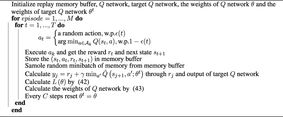 Through Algorithm 2, a Q value fitting network can be built and trained. With the fitting network, each time the edge node makes a status update control decision under a certain system state, it obtains a state-action pair. Traversing the action space, it obtains all possible “state-action” pairs. By inputting each “state-action” pair into the fitting network, we can obtain the corresponding Q value through the network output. The edge node follows this decision-making method to ensure the minimum system cost in each time slot, so as to ensure the minimum long-term cumulative cost with the optimal policy.
5 Simulation result
In this study, we evaluate our proposed method using the dataset provided by the Intel Berkeley Research laboratory (
Bodik et al., 2004). The dataset contains the real location and the measured temperature of 45 sensors. We use their real location information and measured temperature information for simulation. In this study, we compare its performance with those of several conventional status update control policies to show the superiority of the algorithm proposed in this study. We compare with the following baseline policies:
• Random: The edge node will select a random action ak(t) ∈ {0, 1} in each time slot.
• Greedy: In any time slot, when the user requests information, i.e., rk(t) = 1, the edge node will ask the sensor to update the information, i.e., ak(t) = 1.
• Threshold: When the user requests information I(xk, t), the edge node sends a status update request to the corresponding sensor only when Δk(t) is greater than a given threshold.
In each time slot, the probability of harvesting a unit of energy is denoted by gk, i.e., gk = Pr{hk(t) = 1}. In addition, the user request probability is denoted by pk, i.e., pk = Pr{rk(t) = 1}. For each method, the average cost is defined aswhere is obtained from Eq. 16.
5.1 Ideal channel case
We use the parameter settings shown in Table 1 to verify the performance difference between the algorithm based Q-learning proposed in Section 3.3 and the baseline policies.
TABLE 1
| Parameter | Value |
|---|---|
| number of time slots T | 5 × 10⁷ |
| number of sensors K | 10 |
| user request frequency pk | 0.3 |
| energy harvesting frequency gk | 0.5 |
| weight coefficient β | 0.6 |
| discount factor γ | 0.99 |
| learning rate α | 0.01 |
| exploration rate ϵ |
Simulation parameters of the nonideal channel model.
Figure 5 is the comparison of the average cost of the Q-learning algorithm and the baseline policies with the ideal channel model. It can be seen that the proposed algorithm can converge and is significantly better than other baseline policies. The average cost caused by the threshold policy is slightly lower than that caused by the greedy policy, but both strategies are significantly better than the random policy. Our proposed Q-learning algorithm results in a 1.5-times lower cost than that produced by the threshold policy. At the beginning of learning, the performance of the proposed policy is similar to that of the random policy but gradually increases to a lower level. This changing trend also meets the assumption of the ϵ-greedy strategy, that is, more random actions are selected at the beginning of learning and experience is then used to continuously improve the policy.
FIGURE 5
As shown in Figure 6, the influence of the weight coefficient on the average cost can be observed by changing the weight value β in the cost function. The larger the value of β, the greater is the corresponding average cost. The reason is that in the cost function defined in this study, the energy cost is not strongly related to the user request. If there is no user request and the edge node commands the sensor to update the status, there will be energy cost without information accuracy cost. When a user request occurs and the status of the sensor is updated, it will also result in energy consumption cost without information accuracy cost.
FIGURE 6
To study the influence of different user request frequencies and EH frequencies on the policy proposed in this study, we fix the EH frequency ( and ) and change the user request frequency and obtain the results as shown in Figure 7A. When the user request frequency is constant ( and ) while the EH frequency changes, the result is as shown in Figure 7B. It can be seen that a higher EH frequency and lower user request frequency can reduce the average cost. A high EH frequency means that the sensor has enough energy to update. On the contrary, when the sensor does not have enough energy to update, it will lead to a higher average cost of the system. At the same time, a lower user request frequency means a lower interaction frequency between the user and the system, which also indicates a lower average cost. In general, the algorithm proposed in this section has better performance in the case of fewer user requests and more energy.
FIGURE 7
We also study the differences in energy cost and information accuracy between the proposed method and the baseline policies. As shown in Figure 8, the ratio of energy consumed by the status update to the total energy and the ratio of user request information with an accuracy of 95% to the total user request information are the best in both aspects. It can be seen that the greedy policy will cause a lot of energy costs due to the high update frequency. However, due to the large energy cost, sometimes there is not enough energy to respond to the user’s request. Hence, it results in high information accuracy errors. The threshold policy performs well in energy saving. However, due to its low update frequency, the threshold policy results in more information errors. Because the proposed method will use the cached information to estimate the user’s request information, it can reduce the energy cost and ensure information accuracy.
FIGURE 8
5.2 Nonideal channel case
By implementing the model described in Section 4.1 and simulating with the parameters mentioned in Table 2, the transition probability matrix between the channel states of the nonideal channel model can be obtained as follows:
TABLE 2
| Parameter | Value |
|---|---|
| average signal-to-noise ratio | 15 dB |
| Doppler frequency fd | 10 Hz |
| slot length per frame Tf | 2 ms |
| number of channel states N | 5 |
| fading parameters m | 1 |
| number of bits per packet M | 1,080 |
Simulation parameters of the nonideal channel model.
The simulation parameters of the experiment are shown in Table 3.
TABLE 3
| Parameter | Value |
|---|---|
| memory buffer size | 2000 |
| samples per batch | 250 |
| target network parameter update cycle | 125 |
| number of sensors K | 10 |
| user request frequency pk | 0.3 |
| energy harvesting frequency gk | 0.5 |
| weight coefficient β | 0.6 |
| discount factor γ | 0.99 |
| learning rate α | 0.01 |
| exploration rate ϵ |
Simulation parameters of the ideal channel model.
As shown in Figure 9, the loss function value of training gradually converges.
FIGURE 9
Figure 10 shows the comparison of the average cost between the DQN-based algorithm and several baseline policies. It can be seen that with sufficient training rounds, the results of DQN can converge and are better than those of the baseline policies. In addition, the performance of two different channel detection schemes is compared. The results show that the energy cost of each channel detection has a great impact on the two schemes. When the energy cost of each channel detection is small (ED = 1), the decision-making method of channel detection at the beginning of each time slot is slightly better than the one of using a historical channel state. It is advantageous to use the latest channel state information for decision-making, but it will cause more energy costs because all sensor channel states need to be detected at the beginning of each time slot. Therefore, compared with the use of historical channel states, channel state detection at the beginning of each time slot shows better performance with low channel detection energy cost. With the increase in the energy cost of channel detection, the average cost of the OCSCD for channel detection at the beginning of each time slot becomes greater than that of the OCSCD using historical channel state information. When the energy cost of channel detection continues to increase to 3, the average cost of channel detection at the beginning of the time slot is even greater than that of the baseline policies. This indicates that when the energy cost of channel detection is large, using the OCSCD scheme is unfavorable for decision-making. Channel detection at the beginning of each time slot may consume a large amount of energy, so that the sensor does not have enough energy to update the status.
FIGURE 10
Figure 11 shows the information accuracy cost and energy of the proposed method and baseline policies under different user request frequencies. It can be seen that the algorithm proposed in this study is optimal.
FIGURE 11
This study also presents statistics on the channel usage frequency of each policy under different user request frequencies, and the results are shown in Figure 12. Using the ratio of the total number of status updates of the sensor to the total number of channels with good channel state in all time slots as the statistical standard, it can be seen that the proportion of the number of updates of the method proposed in this study is the smallest; with the increase in the user’s request frequency, the use of state correlation for state estimation is more helpful to reduce the frequency of sensor status updates. It can be seen from the figure that the performance gain of the method proposed in this study is the most obvious under the high user request frequency. This is because when the overall network information cached by the edge node is relatively fresh, higher information accuracy can be guaranteed through the cached information or estimated information for some time, so as to reduce the update frequency of the whole sensor network and save more energy.
FIGURE 12
6 Conclusion
This study analyzes how to use the correlation between sensor status updates to ensure the accuracy of sensor observation results and reduce the energy cost in a network composed of EH sensors. The status information is spatiotemporally related for all sensors. Therefore, status updates from some sensors are helpful when estimating the status information of others. Two channel models are considered in this study. In the ideal channel model, the communication channels between the sensor and the edge node are independent and in good condition. In the nonideal channel model, all the sensors share a limited number of channels and the channel state is time-varying, which requires sensors to communicate with edge nodes with different power. By transforming the decision control problem under the two models into a multi-objective control decision problem with Markov property, the control policy is solved by an algorithm based on RL. Using a dataset obtained from a real sensor network, the simulation results show that the control policy proposed in this study outperforms the baseline policies. In addition, the simulation results show that energy balance can be achieved to a certain extent, i.e., the edge nodes will command the sensors with higher energy costs to update the state more frequently.
Statements
Data availability statement
Publicly available datasets were analyzed in this study. This data can be found here: http://db.csail.mit.edu/labdata/labdata.html.
Author contributions
ZH prepared the code, performed the simulation, and wrote the first draft. JG provided the research ideas and revised the first draft.
Funding
The work is supported in part by the NSFC (No. 62171481), the Special Support Program of Guangdong (No. 2019TQ05X150), and the Natural Science Foundation of Guangdong Province (No. 2021A1515011124).
Conflict of interest
The authors declare that the research was conducted in the absence of any commercial or financial relationships that could be construed as a potential conflict of interest.
Publisher’s note
All claims expressed in this article are solely those of the authors and do not necessarily represent those of their affiliated organizations, or those of the publisher, the editors, and the reviewers. Any product that may be evaluated in this article, or claim that may be made by its manufacturer, is not guaranteed or endorsed by the publisher.
Footnotes
1.^The study was partially presented in IEEE WCSP (Han and Gong, 2021).
References
1
Abd-ElmagidM. A.PappasN.DhillonH. S. (2019). On the role of age of information in the internet of things. IEEE Commun. Mag.57, 72–77. 10.1109/MCOM.001.1900041
2
Abd-ElmagidM. A.DhillonH. S.PappasN. (2020b). A reinforcement learning framework for optimizing age of information in RF-powered communication systems. IEEE Trans. Commun.68, 4747–4760. 10.1109/TCOMM.2020.2991992
3
Abd-ElmagidM. A.DhillonH. S.PappasN. (2020a). AoI-optimal joint sampling and updating for wireless powered communication systems. IEEE Trans. Veh. Technol.69, 14110–14115. 10.1109/TVT.2020.3029018
4
AhlgrenB.HidellM.NgaiE. C.-H. (2016). Internet of things for smart cities: Interoperability and open data. IEEE Internet Comput.20, 52–56. 10.1109/MIC.2016.124
5
Ait AoudiaF.GautierM.BerderO. (2018). Rlman: An energy manager based on reinforcement learning for energy harvesting wireless sensor networks. IEEE Trans. Green Commun. Netw.2, 408–417. 10.1109/TGCN.2018.2801725
6
[Dataset]BodikP.HongW.GuestrinC.MaddenS.PaskinM.ThibauxR. (2004). Intel lab data.
7
ChuY.MitchellP. D.GraceD. (2012). “ALOHA and Q-Learning based medium access control for wireless sensor networks,” in 2012 International Symposium on Wireless Communication Systems (ISWCS), 511–515. 10.1109/ISWCS.2012.6328420
8
CressieN.HuangH.-C. (1999). Classes of nonseparable, spatio-temporal stationary covariance functions. J. Am. Stat. Assoc.94, 1330–1339. 10.1080/01621459.1999.10473885
9
FangW.SongX.WuX.SunJ.HuM. (2017). Novel efficient deployment schemes for sensor coverage in mobile wireless sensor networks. Inf. Fusion41, 25–36. 10.1016/j.inffus.2017.08.001
10
FeiX.BoukercheA.YuR. (2010). “A POMDP based K-coverage dynamic scheduling protocol for wireless sensor networks,” in 2010 IEEE Global Telecommunications Conference GLOBECOM 2010, 1–5. 10.1109/GLOCOM.2010.5683311
11
FizzaK.BanerjeeA.MitraK.JayaramanP. P.RanjanR.PatelP.et al (2021). QoE in IoT: A vision, survey and future directions. Discov. Internet Things1, 4. 10.1007/S43926-021-00006-7
12
GindullinaE.BadiaL.GündüzD. (2021). Age-of-information with information source diversity in an energy harvesting system. IEEE Trans. Green Commun. Netw.5, 1529–1540. 10.1109/TGCN.2021.3092272
13
HanZ.GongJ. (2021). “Correlated status update of energy harvesting sensors based on reinforcement learning,” in 2021 13th International Conference on Wireless Communications and Signal Processing (WCSP), 1–5. 10.1109/WCSP52459.2021.9613332
14
HatamiM.JahandidehM.LeinonenM.CodreanuM. (2020). “Age-aware status update control for energy harvesting IoT sensors via reinforcement learning,” in 2020 IEEE 31st Annual International Symposium on Personal, Indoor and Mobile Radio Communications, 1–6. 10.1109/PIMRC48278.2020.9217302
15
HribarJ.MarinescuA.ChiumentoA.DaSilvaL. A. (2021). Energy aware deep reinforcement learning scheduling for sensors correlated in time and space. IEEE Internet Things J.1, 6732–6744. 10.1109/JIOT.2021.3114102
16
HribarJ.MarinescuA.RopokisG. A.DaSilvaL. A. (2019). “Using deep Q-learning to prolong the lifetime of correlated internet of things devices,” in 2019 IEEE International Conference on Communications Workshops (ICC Workshops), 1–6. 10.1109/ICCW.2019.8756759
17
LengS.YenerA. (2019). Age of information minimization for an energy harvesting cognitive radio. IEEE Trans. Cogn. Commun. Netw.5, 427–439. 10.1109/TCCN.2019.2916097
18
LiF.LamK.-Y.ShengZ.ZhangX.ZhaoK.WangL.et al (2018). Q-learning-based dynamic spectrum access in cognitive industrial internet of things. Mob. Netw. Appl.23, 1636–1644. 10.1007/s11036-018-1109-9
19
LiH.WangS.GongM.ChenQ.ChenL. (2017). IM 2 dca: Immune mechanism based multipath decoupling connectivity algorithm with fault tolerance under coverage optimization in wireless sensor networks. Appl. Soft Comput.58, 540–552. 10.1016/j.asoc.2017.05.015
20
LiuQ.ZhouS.GiannakisG. (2005). Queuing with adaptive modulation and coding over wireless links: Cross-layer analysis and design. IEEE Trans. Wirel. Commun.4, 1142–1153. 10.1109/TWC.2005.847005
21
MitraR.KhanT. (2013). “Improving wireless sensor network lifetime through power aware clustering technique,” in Fifth International Conference on Advances in Recent Technologies in Communication and Computing (ARTCom 2013), 382–387. 10.1049/cp.2013.2240
22
MnihV.KavukcuogluK.SilverD.GravesA.AntonoglouI.WierstraD.et al (2013). Playing atari with deep reinforcement learning. arXiv Prepr. arXiv:1312.5602. 10.48550/arXiv.1312.5602
23
PappasN.ChenZ.HatamiM. (2020). “Average aoi of cached status updates for a process monitored by an energy harvesting sensor,” in 2020 54th Annual Conference on Information Sciences and Systems (CISS), 1–5. 10.1109/CISS48834.2020.1570629110
24
PaszkeA.GrossS.MassaF.LererA.ChintalaS. (2019). Pytorch: An imperative style, high-performance deep learning library. arXiv:1912.01703. 10.48550/arXiv.1912.01703
25
RazavilarJ.LiuK.MarcusS. (2002). Jointly optimized bit-rate/delay control policy for wireless packet networks with fading channels. IEEE Trans. Commun.50, 484–494. 10.1109/26.990910
26
SchizasI. D.GiannakisG. B.RoumeliotisS. I.RibeiroA. (2008). Consensus in ad hoc WSNs with noisy links-part ii: Distributed estimation and smoothing of random signals. IEEE Trans. Signal Process.56, 1650–1666. 10.1109/TSP.2007.908943
27
StamatakisG.PappasN.TraganitisA. (2019). “Control of status updates for energy harvesting devices that monitor processes with alarms,” in 2019 IEEE Globecom Workshops (GC Wkshps), 1–6. 10.1109/GCWkshps45667.2019.9024463
28
SteinM. L. (2005). Space–time covariance functions. J. Am. Stat. Assoc.100, 310–321. 10.1198/016214504000000854
29
StüberG. L.SteuberG. L. (1996). Principles of mobile communication, vol. 2. Berlin, Germany: Springer. 10.1007/978-1-4614-0364-7
30
SuttonR.BartoA. (1998). Reinforcement learning: An introduction. IEEE Trans. Neural Netw.9, 1054. 10.1109/TNN.1998.712192
31
WolfertS.GeL.VerdouwC.BogaardtM.-J. (2017). Big data in smart farming–a review. Agric. Syst.153, 69–80. 10.1016/j.agsy.2017.01.023
32
XuL. D.HeW.LiS. (2014). Internet of things in industries: A survey. IEEE Trans. Ind. Inf.10, 2233–2243. 10.1109/TII.2014.2300753
33
YacoubM.BautistaJ.Guerra de Rezende GuedesL. (1999). On higher order statistics of the nakagami-m distribution. IEEE Trans. Veh. Technol.48, 790–794. 10.1109/25.764995
34
YangJ.WuX.WuJ. (2015). Optimal scheduling of collaborative sensing in energy harvesting sensor networks. IEEE J. Sel. Areas Commun.33, 512–523. 10.1109/JSAC.2015.2391971
35
YatesR. D.KaulS. K. (2019). The age of information: Real-time status updating by multiple sources. IEEE Trans. Inf. Theory65, 1807–1827. 10.1109/TIT.2018.2871079
36
ZhengJ.CaiY.ShenX.ZhengZ.YangW. (2015). Green energy optimization in energy harvesting wireless sensor networks. IEEE Commun. Mag.53, 150–157. 10.1109/MCOM.2015.7321985
37
ZhuH.CaoY.WeiX.WangW.JiangT.JinS.et al (2019). Caching transient data for internet of things: A deep reinforcement learning approach. IEEE Internet Things J.6, 2074–2083. 10.1109/JIOT.2018.2882583
Summary
Keywords
Internet of Things, wireless sensor network, energy harvesting, age of information, reinforcement learning
Citation
Han Z and Gong J (2022) Status update control based on reinforcement learning in energy harvesting sensor networks. Front. Comms. Net 3:933047. doi: 10.3389/frcmn.2022.933047
Received
30 April 2022
Accepted
13 July 2022
Published
31 August 2022
Volume
3 - 2022
Edited by
Nikolaos Pappas, Linköping University, Sweden
Reviewed by
Mohamed Abd-Elmagid, Virginia Tech, United States
Mohammad Hatami, University of Oulu, Finland
Updates
Copyright
© 2022 Han and Gong.
This is an open-access article distributed under the terms of the Creative Commons Attribution License (CC BY). The use, distribution or reproduction in other forums is permitted, provided the original author(s) and the copyright owner(s) are credited and that the original publication in this journal is cited, in accordance with accepted academic practice. No use, distribution or reproduction is permitted which does not comply with these terms.
*Correspondence: Jie Gong, gongj26@mail.sysu.edu.cn
This article was submitted to Wireless Communications, a section of the journal Frontiers in Communications and Networks
Disclaimer
All claims expressed in this article are solely those of the authors and do not necessarily represent those of their affiliated organizations, or those of the publisher, the editors and the reviewers. Any product that may be evaluated in this article or claim that may be made by its manufacturer is not guaranteed or endorsed by the publisher.