The utility of dynamic forest structure from GEDI lidar fusion in tropical mammal species distribution models

Remote sensing is an important tool for monitoring species habitat spatially and temporally. Species distribution models (SDM) often rely on remotely-sensed geospatial datasets to predict probability of occurrence and infer habitat preferences. Lidar measurements from the Global Ecosystem Dynamics Investigation (GEDI) are shedding light on three dimensional forest structure in regions of the world where this aspect of species habitat has previously been poorly quantified. Here we combine a large camera trap dataset of mammal species in Borneo and Sumatra with a diverse set of geospatial data to predict the probability of occurrence of 47 species. Multi-temporal GEDI predictors were created through fusion with Landsat time series, extending back to the year 2001. The availability of these GEDI-based forest structure predictors and other temporally-resolved predictor variables enabled temporal matching of species occurrences and hindcast predictions of species probability of occurrence at years 2001 and 2021. Our GEDI-Landsat fusion approach worked well for forest structure metrics related to canopy height (relative height of the 95th percentile of returned energy R² = 0.62 and relative RMSE = 41%) but, not surprisingly, was less accurate for metrics related to interior canopy vegetation structure (e.g., plant area volume density from 0 to 5 m above the ground R² = 0.05 and relative RMSE = 85%). For the SDM analyses, we tested several combinations of predictor sets and found that when considering a large pool of multiscale predictors, the exact composition, and whether GEDI Fusion predictors were included, didn’t have a large impact on generalized linear modeling (GLM) and Random Forest (RF) model performance. Adding GEDI Fusion predictors to a baseline set only meaningfully improved performance for some species (n = 4 for RF and n = 3 for GLM). However, when GEDI Fusion predictors were used in a smaller predictor set that is more suitable for hindcasting species probability of occurrence, more SDMs showed meaningful performance improvements relative to the baseline model (n = 9 for RF and n = 4 for GLM) and the relative importance of GEDI-based canopy structure predictors increased relative to when they were combined with the baseline predictor set. Moreover, as we examined predictor importance and partial dependence, the utility of GEDI Fusion predictors in hindcast models was evident in regards to ecological interpretability. We produced a catalog of probability of occurrence maps for all 47 mammals species at 90 m spatial resolution for years 2001 and 2021, enabling subsequent ecological interpretation and conservation analyses.

1 Introduction

Global terrestrial biodiversity loss over the last several decades has been driven primarily by land use change (urbanization and conversion to agriculture), forest degradation and deforestation, direct exploitation (hunting and wildlife trade), and to a lesser degree by pollution, climate change, and invasive alien species (Jaureguiberry et al., 2022). Currently, approximately 28% of all species are threatened with extinction (IUCN, 2024), which includes relatively well-studied vertebrates (∼21%) and mammals (∼26%). Many of these threatened and endangered species are experiencing declining population trends due to decreasing forest structural condition and the impacts of human pressure (Pillay et al., 2024). Understanding spatiotemporal species distributions in the context of the drivers of biodiversity collapse is particularly important for monitoring and conservation of key habitats. Species distributions are influenced by a variety of interacting and often related factors, including, but not limited to, availability of food/water, (micro)climate, geomorphology, anthropogenic influence/disturbance (e.g., hunting, pollution, land conversion), as well as vegetation composition and three-dimensional (3D) structure. Many of these factors can be represented by remotely-sensed geospatial datasets (Turner et al., 2003; He et al., 2015). Such data can be coupled with species observations in various statistical or machine learning modeling frameworks, commonly referred to as environmental niche or species distribution models (SDMs). SDMs are widely applied to make inferences about species habitat preferences and to predict species occurrence spatially and temporally (Elith and Leathwick, 2009; Dormann et al., 2012).

Geospatial datasets derived from remote sensing have played an important role in SDMs because they represent ecologically relevant features of the landscape (e.g., climate, geomorphology, vegetation type/structure), often in a spatially and temporally continuous manner (Randin et al., 2020). Two-dimensional imagery recorded by passive optical instruments (e.g., Landsat) has been very useful for mapping vegetation extent and species habitats (Valerio et al., 2020; Crego et al., 2024), especially when considering changes in habitat due to forest degradation or loss (Betts et al., 2022). Unfortunately, in dense forests these passive optical observations only correspond to reflectance of the upper portion of the canopy. However, the entire vertical dimension of forests, which may be characterized by metrics like canopy height, foliage height diversity (MacArthur and MacArthur, 1961), canopy cover and leaf/plant area index (LAI/PAI) profiles, often influences habitat selection, especially for arboreal species (Davies and Asner, 2014). These relationships arise because vertical forest structure is linked to available niche space (Deere et al., 2020), light and water availability (Montgomery and Chazdon, 2001; Wüest et al., 2020), as well as microclimate (Hardwick et al., 2015; Zellweger et al., 2019). Furthermore, high forest integrity, which incorporates canopy structure as well as human pressure, is associated with a lower likelihood of species being threatened and having declining populations versus canopy cover alone (Pillay et al., 2022).

The Global Ecosystem Dynamics Investigation (GEDI) (Dubayah et al., 2020), a current spaceborne NASA mission, provides an opportunity to characterize the vertical dimension of forests across the tropics and mid-latitudes using lidar. The instrument acquired data from April 2019 to March 2023, and then resumed lidar waveform acquisition in April 2024. Several studies have already demonstrated the utility of the unique data GEDI provides in understanding animal-habitat associations, including species occupancy (Killion et al., 2023; Martins et al., 2024) and distribution models (Burns et al., 2020; Smith et al., 2022; Vogeler et al., 2023). Thus far, the GEDI mission has provided >7 billion high-quality vertical vegetation structure measurements between the latitudes of 52° North and South. Importantly, the sensor is capable of accurately measuring various structural properties of dense tropical forests at a sampled spatial resolution of 25 m. Lidar waveforms are acquired below the path of the International Space Station orbit and are spaced by about 60 m along track and 600 m across track. The observation strategy of GEDI and the resulting gaps at fine spatial resolutions (<1 km) have implications for applied studies making use of GEDI data. One common method for converting lidar observations (i.e., points) to continuous layers (i.e., rasters) which are more convenient for use in SDMs is gridding, that is, lidar observations in a pixel are summarized using statistics, like the mean and standard deviation. Currently, in most parts of the tropics gridding is not a viable option since many 1 km spatial resolution pixels have fewer than 10 high-quality GEDI observations (Burns et al., 2024). Gap-free, fine-resolution maps are necessary for associating vegetation structure with in situ data (e.g., forest plots, camera traps, acoustic recording units) and understanding ecological patterns across broad landscapes. Fortunately, several previous studies have demonstrated the capability of machine and deep learning for fusing GEDI and optical satellite imagery (i.e., using 2D imagery to predict 3D structure) from Landsat, Sentinel-1, and Sentinel-2 for achieving continuous maps of forest structure across entire landscapes. Several studies have produced global fusion maps of canopy height (Potapov et al., 2021; Lang et al., 2023), while relatively few studies have explored the efficacy of fusion for mapping sub-canopy metrics such as the height of median returned energy or the amount of foliar material in different layers of the canopy (Vogeler et al., 2023). With the exception of canopy cover (Sexton et al., 2013), stand-clearing disturbances (Hansen et al., 2013), and degradation (Vancutsem et al., 2021), the temporal dynamics of forest structure have also been challenging to represent over large extents in the tropics since lidar data in the region were sparse or non-existant prior to the GEDI mission.

In this study we explore the utility of GEDI lidar fusion for SDMs, focusing on the equatorial islands of Sumatra and Borneo which are part of the Sundaland biodiversity hotspot - a region home to an estimated 1,800 vertebrate species, of which 701 are endemic (Myers et al., 2000). Of the 1241 terrestrial bird, reptile, amphibian and mammal species cataloged by the IUCN Red List in Borneo and Sumatra, 91% use forest habitat to some degree. Mammal species (n = 277), the taxonomic focus of this study, are even more closely linked to forest habitat in this region, with 97% of them using forest habitats (IUCN, 2024). The forests of Sundaland are characterized by extremely high floristic and structural diversity, and include the tallest known tropical forest trees (Shenkin et al., 2019; Milodowski et al., 2021). This region has experienced some of the highest rates of deforestation and degradation in the world - 48.5% (Malaysia) and 38.7% (Indonesia) of undisturbed tropical moist forest area disappeared since 1990 from continuous deforestation and forest degradation (Vancutsem et al., 2021). Considering the magnitude of forest loss and degradation and the number of species that use forest habitat in this region, various groups have advanced data-driven ecological modeling and conservation design optimization over the past decade in the Sundaland region, facilitated by coupling data from camera trap networks (Hearn et al., 2018; Macdonald et al., 2019a; Ke and Luskin 2019; Brodie et al., 2023) with multiscale statistical modeling (Chiaverini et al., 2022; 2023) and scenario optimization (Kaszta et al., 2019; 2020; 2024; Macdonald et al., 2024). These studies have evaluated habitat relationships of focal species of conservation concern (Amir et al., 2022; Mohd-Azlan et al., 2023; Honda et al., 2024; Panjang et al., 2024), mapped and optimized networks of protected areas (Scriven et al., 2020; Williams et al., 2020; Macdonald et al., 2024) and ecological connectivity (Brodieet al., 2016; Hearn et al., 2019; Kaszta et al., 2019; 2024), assessed impacts of climate change (Brodie et al., 2017), hunting (Brodie et al., 2015), and logging (Wall et al., 2021; Yi et al., 2022), and evaluated multiple scenarios of conservation design and development impact (Williams et al., 2020; Kaszta et al., 2020; 2024). With the exception of Brodie et al. (2023), none of this past work considered vertical vegetation structure metrics. The extreme gradients of vegetation diversity and structure in Sundaland, and the strong association of the resident wildlife species to forested environments of varying characteristics, justify a critical evaluation of the extent to which remotely-sensed vertical forest structure information can improve predictions of species distributions and provide novel ecological insights about habitat preferences.

Here we incorporate multiple dimensions of forest structure (horizontal, height above ground, and time) to better understand and dynamically map the distribution of mammal species in Borneo and Sumatra. Integrating the temporal dimension is possible through fusion of GEDI lidar metrics with Landsat continuous change detection and classification (CCDC) (Zhu and Woodcock, 2014) time series, enabling the prediction of forest structure metrics continuously at relatively fine spatial resolution (hereafter referred to as “GEDI Fusion”), both during the time of the GEDI mission and back to the year 2001 (i.e., hindcasting). The species occurrence data used in this work originate from an extensive compilation of camera trap sites over nearly 2 decades (2003-2022). Considering the years of species occurrence observations and the area of forest lost in this region, hindcasting is a vital method for temporally-matching forest structure with species occurrence. We also make use of other multitemporal, multiscale geospatial predictors characterizing geomorphology, climate, productivity, disturbance, and human influence. Furthermore, we compare and contrast different model scenarios, which make use of different groups of predictors, for understanding the utility of GEDI Fusion metrics and changes in species probability of occurrence over time.

The three specific objectives of this study are to 1) develop and validate continuous forest structure maps derived from fusion of GEDI lidar metrics and Landsat CCDC, 2) assess the utility of GEDI Fusion predictors in SDMs, in terms of model performance, predictor importance, and general interpretability, and 3) map the predicted probability of occurrence for 47 mammal species at two time periods, 2001 and 2021.

2 Materials and methods

2.1 Study region

We focus on the islands of Sumatra and Borneo, part of the Sundaland biodiversity hotspot. The islands are divided among Indonesia, Malaysia, and Brunei, and are home to over 60 million people. Importantly, we treat each island as a separate modeling domain considering potential differences in human influence and species composition, as well as camera trap survey effort. The approximate locations of camera traps and recent, modeled forest structure dynamics are shown in Figure 1.

Figure 1

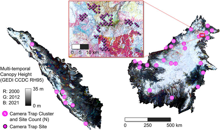
Figure 1. Map of study region, including multi-temporal GEDI Fusion canopy height (RH95) as the background. GEDI Fusion RH95 from 3 years (2000, 2012, 2021) is displayed in the red, green, and blue channels of the background image. Hence, colors correspond to areas of canopy height change. For example, red represents the presence of relatively tall forests in 2000, but not in 2012 or 2021. Hence loss of tall forest occurred some time between 2000 and 2011. Black and white correspond to consistent low and high canopy height, respectively. Camera trap clusters are shown as magenta circles with white text corresponding to site count. The inset image is zoomed in on a cluster of individual camera trap sites.

2.2 Species occurrence dataset

The species occurrence records used in this study were acquired using camera traps. Camera traps were deployed and processed by several teams (Macdonald et al., 2018; 2019b; Williams et al., 2022; Brodie et al., 2023; Luskin et al., 2023; Mohd-Azlan et al., 2023). We merged these datasets and harmonized species names, focusing on 47 mammal species (Table 1). Based on the IUCN Red List, 11 of the species modeled in this study are endangered (IUCN, 2024). Three species, the Bornean orangutan, Sunda pangolin, and Sumatran tiger, are critically endangered (Luskinet al., 2017; Amir et al., 2022; Voigt et al., 2022; Nursamsi et al., 2023). The subspecies of the Asian elephant in Sumatra (Elephas maximus sumatranus) are also critically endangered, but there were insufficient observations to model this species. Five species have stable populations, while 40 have declining populations, and for two species’ population trends are unknown.

Table 1

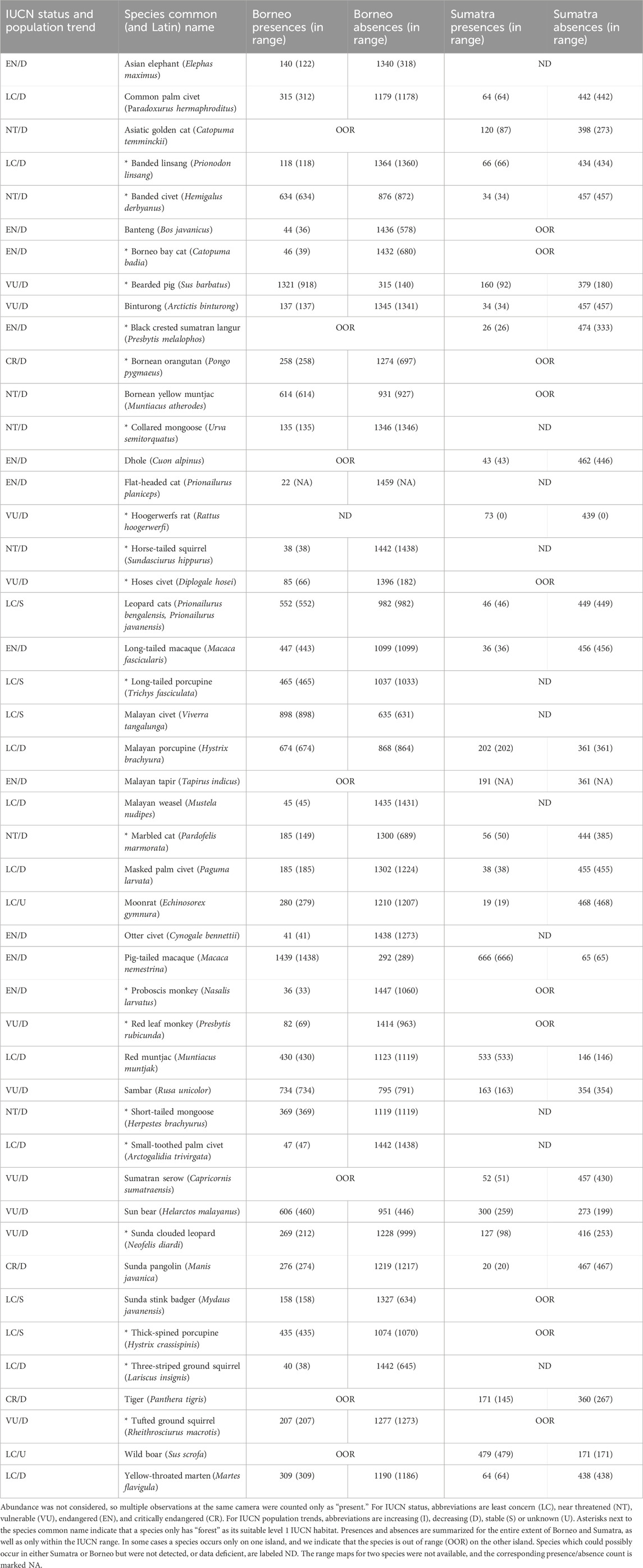
Table 1. List of all species considered, IUCN status and population trend, and number of presences and absences considering all camera trap sites in each region and considering only sites within IUCN species range maps (extant and possibly extant; version 6.3).

Following the merging of camera trap datasets, there were 2,023 sites in Borneo and 879 sites in Sumatra. The survey effort, or median number of camera trap nights, was higher in Borneo (56) than Sumatra (34) (Supplementary Figures S1, S2). A species was considered present at a site if it was manually identified in at least one photograph. Absences are more challenging to establish due to the imperfect detectability of species in dense forests and the placement of cameras near the ground. We use a threshold of 30 camera trap nights to establish absence. The lowest number of presences was for moonrats in Sumatra (n = 19), while the highest was for pig-tailed macaques in Borneo (n = 1,439). In Table 1 we quantify presences and absences for each species considering all camera trap sites in each region and considering only sites within IUCN species range maps.

2.3 Geospatial datasets used as predictors SDMs

We prepared multi-scale and multi-temporal predictor variable rasters in Google Earth Engine (GEE) (Gorelick et al., 2017) and extracted values at camera trap locations. These predictors were used to inform two predictive modeling algorithms: logistic regression with generalized linear modeling (GLM) and machine learning with Random Forest (RF) (Breiman, 2001). The complete list of predictors is provided in Supplementary Table S1, and below we provide a brief overview of the different predictor groups and associated datasets.

2.3.1 Climate

Climate predictors are spatial and temporal aggregations of meteorological observations or outputs from climate models. These types of predictors are not readily available at spatial resolutions finer than approximately 1 km and therefore this set of predictors does not characterize microclimate (Lembrechts et al., 2019). Furthermore, while climate predictors are becoming increasingly available at finer temporal resolutions, it is still common practice to make use of long term climate averages (climatologies) in SDMs. The majority of climate predictors we used in this study are from the CHELSA Bioclim + dataset (Karger et al., 2017; 2018). We also included cloud cover (Wilson and Jetz, 2016) and land surface temperature predictors derived from MODIS (Zhang et al., 2022).

2.3.2 Geomorphology

Geomorphology predictors are selected to represent features of the Earth’s surface, like ground elevation, slope, landform types, hydrology, and soil properties. Most features associated with topography are mapped at approximately 100 m spatial resolution (Theobald et al., 2015; Amatulli et al., 2020), while soil properties have been modeled globally at 250 m spatial resolution (Poggio et al., 2021). Surface water has been mapped annually at 30 m spatial resolution using Landsat, but some small extent water features may be obscured under/in the proximity of dense tropical forests (Pickens et al., 2022).

2.3.3 Human influence

There are a variety of human pressures that influence species distributions in this region of the world, such as urbanization, conversion of forest to agriculture, and hunting. We used 1 km spatial resolution gridded world population, 1 km gross domestic product (GDP) (Chen and Gao, 2021), and an index of human modification at 300 m spatial resolution (Theobald et al., 2023) as general proxies for human influence. Potential hunting pressure is characterized using a human accessibility map developed specifically for this region at 1 km spatial resolution (Deith and Brodie, 2020; Brodie et al., 2023). Lastly, we used three separate binary datasets to represent croplands other than oil palm plantations at 30 m spatial resolution (Potapov et al., 2022), oil palm plantations at 30 m spatial resolution (Descals et al., 2021), and protected areas (UNEP-WCMC and IUCN, 2024) rasterized to 90 m spatial resolution.

2.3.4 Vegetation productivity

Like many of the other predictors, vegetation productivity cannot be measured directly from space. Instead, different algorithms and remote sensing products are used to model either gross or net primary productivity. We used modeled net primary productivity from the CHELSA dataset (Karger et al., 2017; 2018) at 1 km spatial resolution. We also incorporated three dynamic habitat indices (DHI) based on gross primary productivity modeled from MODIS (Radeloff et al., 2019).

2.3.5 Vegetation spectral indices

Vegetation spectral indices are related to plant species community composition, as well as plant chemical traits (e.g., water content, chlorophyll absorption) and density. We used four visible to shortwave (VSWIR) spectral indices derived from Landsat Collection 2 CCDC (Zhu and Woodcock, 2014) synthetic imagery to characterize different vegetation characteristics. Following Landsat cloud-masking, the CCDC algorithm fits harmonic regression equations to a time series of Landsat band/index values. Importantly, CCDC is capable of detecting change points and separating time series segments which may correspond to vegetation stability or regrowth after a disturbance, for example. After fitting CCDC models from 2000 to 2022, we used the harmonic regression equations to generate synthetic images every 3 years (2000, 2003, … ,2021) so that species occurrences could be temporally associated with Landsat spectral indices. Three year intervals are a reasonable choice considering cloud-free Landsat availability and storage volume. We selected a set of spectral indices which make use of spectral bands across the VSWIR spectrum and are less susceptible to variability in illumination, specifically: normalized difference vegetation index (NDVI), normalized burn ratio (NBR), normalized difference moisture index (NDMI), and spectral variability vegetation index (SVVI).

2.3.6 Forest structure derived from GEDI Landsat fusion

Geolocated GEDI waveforms (L1A; Dubayah, Luthcke, et al., 2021) are initially processed to extract ground elevation, vegetation height, relative height (RH) (L2A; Dubayah, Hofton, et al., 2021), and several vertical vegetation profile metrics, such as cover and PAI (L2B; Dubayah, Tang, et al., 2021). We downloaded all available GEDI L2A, L2B, and L4A granules covering Borneo and Sumatra from 17 April 2019 to 13 April 2022. We applied the quality-filtering steps described by Burns et al. (2024) to select the highest quality observations for the region. We selected the following metrics to model: RH50 (Height of Median Energy), RH95 (Canopy Height), Plant Area Index (PAI), Above Ground Biomass Density (AGBD), Foliage Height Diversity (FHD), Cover, and the number of modes in the returned waveform.

Following the quality-filtering, we had millions of GEDI observations to use for fusion with the fit Landsat CCDC time series. However, preliminary testing suggested that this was an excessive number of observations to use for model training. Furthermore, we observed some GEDI clustering due to cloud cover dynamics and ISS orbital resonance patterns. For these reasons we developed a subsampling routine to reduce the number of observations used for model training and validation. Furthermore, we sought to account for spatial autocorrelation when assessing model error by incorporating a 30 × 30 km grid for separating GEDI observations for training and validation of the model. We randomly partitioned 70% of the 30 km grids for training and 30% for validation. Next, we examined semivariograms of several GEDI structure metrics to estimate an approximate range (distance in meters) at which GEDI metrics were not autocorrelated; we estimated this range to be 10 km (see Supplementary Figure S3). To ensure that no validation observations fell within the spatial autocorrelation range (distance) of training observations, we inversely buffered testing grids by 10 km and only selected GEDI observations within the resulting 10 × 10 km grids. To calculate the subsampling threshold per grid, we computed the 10th percentile of the number of observations in grids (minimum of 100 observations). We applied this subsampling threshold to the grids in order to reduce spatial bias (associated with orbit clustering) in the model. We added a random number field and combined all of the subsampled observations into one table and uploaded the table to GEE.

Within GEE we made several adjustments to the previously quality-filtered and subsampled GEDI observations. First, for the GEDI metric relative height of the 95th percentile of returned energy (RH95; proxy for vegetation height) we followed the method of Potapov et al. (2021) and set RH95 to 0 when the measured value is less than or equal to 3 m. Due to the long pulse width of the instrument, GEDI struggles to accurately measure vegetation height less than 3 m tall. Also similar to Potapov et al. (2021), we applied preferential sampling towards the low end of each GEDI metric based on prior knowledge that model predictions based on optical imagery saturate at higher values of most metrics (Gao et al., 2023), especially in dense tropical forests. In other words, we knew it would be unlikely to accurately predict the height of very tall trees, for example, so we emphasized improving the prediction of low values which are often overestimated (Lang et al., 2023). In this vein, we defined five bins using the 20th, 40th, 60th, and 80th percentiles of GEDI metric values as breaks. We specified that 60% of the data should randomly be selected from the first bin, while 10% should be selected from the other 4 bins. The held-out validation data, in contrast, were not preferentially sampled in order to get unbiased error estimates. For each metric, we used approximately 100,000 (75%) observations for training and 33,333 (25%) observations for validation.

Next, we prepared the stack of predictors to be associated with GEDI vertical profiles. The full list is detailed in Supplementary Table S2, but to summarize we used terrain elevation, years since forest loss (from Hansen et al., 2013), and several layers derived from the Landsat CCDC time series. We used the CCDC algorithm in GEE to fit harmonic models to Landsat Collection 2 spectral bands and indices for Borneo and Sumatra. The harmonic model coefficients (offset, t, sin [ωt]), as well as synthetic spectral/index values and texture of select indices, were associated with GEDI observations from Borneo and Sumatra. We created synthetic images every 0.25 years and extracted spectral/index values at GEDI observations when the date of the GEDI shot fell within that quarter year window. Gray level co-occurrence matrix (GLCM) texture metrics were generated from the temporally-matched synthetic images using a 1 pixel radius. The resulting full predictor stack included 48 predictors.

We used the RF algorithm to make spatially-continuous predictions of several GEDI forest structure metrics. To identify the best set of predictors and RF tuning parameters per metric and region we randomly sampled 20,000 observations and extracted values of the predictors described above at 25 m spatial resolution. We then passed these data through the minimum redundancy maximum relevance algorithm (MRMR) (De Jay et al., 2013) feature selection routine in R (R Core Team, 2024) to select a maximum of 20 predictors for each GEDI metric and region. We then used the Ranger (Wright and Ziegler, 2017) implementation of RF via the caret package to tune the RF parameters minimum node size and number of predictors randomly selected at each split (mtry). We passed the best predictors and optimal RF tuning parameters back to GEE and fit RF models with 200 trees for each GEDI metric and region using ∼100,000 observations for training. The fit RF models were then used to make spatial predictions at 90 m resolution for each metric and region.

The spatially-continuous predictions of GEDI Fusion forest structure metrics were evaluated in two ways: using held-out GEDI data and airborne laser scanning (ALS) data. First, we evaluated the predictions at the nominal spatial resolution of GEDI (25 m; i.e., using the validation feature collection) during the original GEDI mission (2019–2022). We computed the root mean square error (RMSE), relative RMSE, as well as mean and median absolute error for each metric. We also computed the R² of a linear model fit to observed vs. predicted metric values where the predicted values were sampled from a raster at the spatial resolution used in SDMs (90 m). Next, since the CCDC algorithm provides harmonic regression equations which can be used to generate synthetic images, the model predictions can either be made during the period of GEDI observation (2019–2022) or hindcasted to previous years that overlap the CCDC harmonic model (2000–2022). A similar methodology for hindcasting forest structure derived from airborne lidar was described by Bell et al. (2024). Since the vast majority of our species occurrence records are from before GEDI began acquiring data, we made GEDI Fusion predictions for the following years, each at January 1: 2000, 2003, 2006, 2009, 2012, 2015, 2018, 2021. As described below, this allowed us to temporally match species occurrences with a set of hindcast GEDI Fusion structure metrics (e.g., an occurrence in 2010 is associated with 2009-01-01). There is limited ALS data in this region to use for assessment of our hindcasted GEDI Fusion predictions, but we were able to compare two high resolution ALS canopy height maps collected in late 2014 (Melendy et al., 2017; Swinfield et al., 2020) with GEDI Fusion RH95 predictions from 2015.

2.4 SDM temporally-matched, multi-scale variable extraction

We developed a workflow in GEE to extract the focal mean, and in some cases standard deviation (see Supplementary Table S1), of predictor variables at multiple spatial scales, to enable multiscale SDM optimization (sensu McGarigal et al., 2016). We used a Gaussian kernel with the GEE reduceNeighborhood method to compute focal mean and standard deviation at seven scales, specified by these radii: 150, 300, 600, 1200, 2400, 4800, and 9600 m to enable multi-scale optimization of habitat selection. Focal statistics are only computed at scales which are coarser than the nominal resolution of the predictor variable. For example, CHELSA climate predictors have a nominal resolution of 1,000 m, so we compute focal statistics at 1,200, 2,400, 4,800, and 9,600 m. Furthermore, and if a predictor variable was temporally-resolved, we temporally-matched the years of species presence/absence with predictor variables (Crego et al., 2021). We created two stacks of multi-scale rasters corresponding to the predictor variables that are temporally-static (e.g., Climate, Geomorphology) or temporally-matchable (e.g., GEDI Fusion). For temporally-static predictors, we simply extracted the multiscale focal values of each predictor at each camera trap location. For the temporally-matched predictors, we filtered predictors which correspond to the species year(s) of occurrence or years in which the camera trap was active in the case of absence, and then computed the temporal mean of those rasters before extracting multi-scale focal values at each camera trap location. Finally, we standardized each multi-scale focal predictor by subtracting the mean and dividing by the standard deviation.

2.5 SDM scenarios

One of the overarching goals of this study was to compare the predictive performance of models built with GEDI Fusion structure metrics to those built without them, as well as other relevant sets which include climate, disturbance, geomorphology, human influence, and productivity predictors. To enable these comparisons we fit models for each species using different subsets of predictor variables (Table 2; Figure 2). Note that when “GEDI Fusion” is included in the name of the predictor set, it refers to GEDI metrics derived from fusion with Landsat CCDC. Also note that all scenarios used the number of camera trap nights at a site as a predictor that represents survey effort. The first, and smallest, set of predictors is “GEDI Fusion.” As the name suggests, this scenario only considers the GEDI structure metrics derived from fusion with Landsat CCDC. The second scenario is “Base,” which is short for baseline, considers all predictors except Landsat CCDC spectral indices and GEDI Fusion metrics. The third scenario is “Base + CCDC Spectral.” Temporally-matched spectral indices derived from Landsat CCDC are added to the Base set of predictors. The fourth scenario, “Base + GEDI Fusion,” swaps GEDI fusion metrics for Landsat CCDC spectral indices, enabling a direct comparison between scenarios three and four. The fifth and final scenario, “Hindcast with GEDI Fusion,” focuses on the highest resolution geomorphology, human influence, disturbance, and GEDI Fusion predictors (marked with asterisks in Supplementary Table S1). For this scenario, we selected predictors which had either high temporal and/or spatial resolution and would be suitable for hindcasting in this region. In this scenario, we notably excluded climate predictors due to their relatively coarse spatial resolution and temporal aggregation over ∼30 years.

Table 2

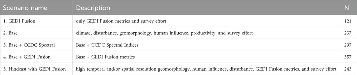
Table 2. Description of the variable composition of different model scenarios and the number of possible predictors (N) considered in each.

Figure 2

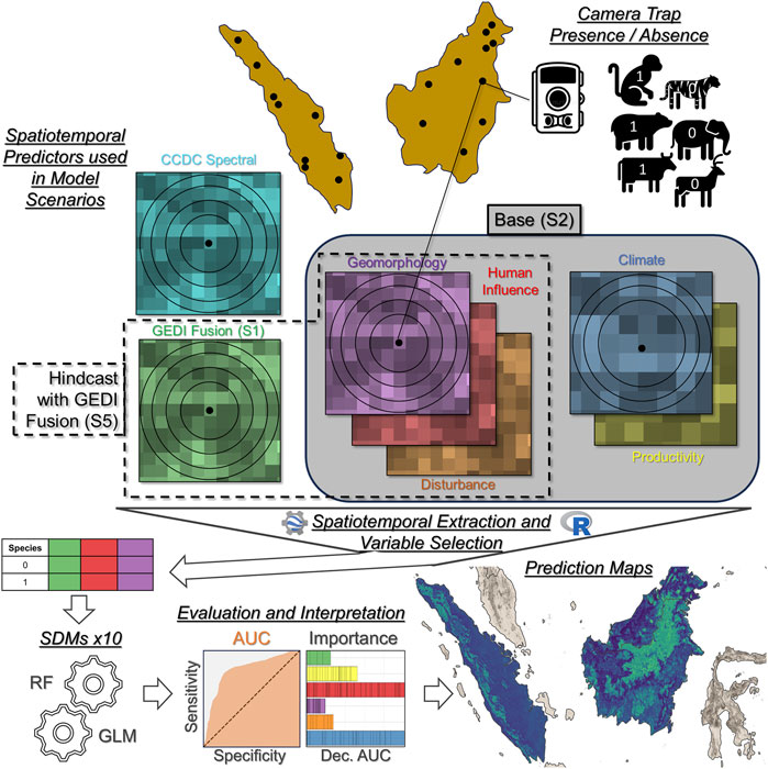
Figure 2. Overview of the workflow for associating species occurrence data from camera traps with multi-scale and multi-temporal geospatial predictors for use in SDMs. The different model scenarios (S1 to S5) make use of different subsets of predictors. Major steps in the workflow are underlined.

2.6 SDM variable selection

Model interpretation can be challenging when there are hundreds of potential predictors, many of which are correlated with each other. The variance inflation factor (VIF) is a commonly used variable selection technique which seeks to remove highly-correlated predictors. We included the option to pre-rank predictors based on a preference order column so that a priori knowledge related to the model outcome (i.e., species absence/presence) could be used to select between pairs of highly-correlated predictors. For each model scenario and predictor we fit univariate GLM and RF models. We chose to use the average of scaled (0–1) GLM Akaike information criterion (AIC) and RF true skill statistic (TSS) for preference order; values are associated with the fit GLM and RF models (i.e., the metrics only consider training data), respectively. We also included the option to compute groupwise VIF (GVIF). Similar to the approach described by Quinn et al. (2024) we used progressively less strict VIF thresholds when moving between the following predictor levels: scale of a single predictor (threshold = 2.5), predictor group (threshold = 5), and full remaining set (threshold = 10). If the GVIF routine resulted in more than 15 selected predictors, we used the average scaled (0–1) univariate AIC/TSS and RF/GLM permutation importance from the R package vip (Greenwell and Boehmke, 2020) to rank the top 15 predictors. Next, for each variable selection method we “dredged” every combination of the top 15 predictors in order to select the 10 best predictors, ideally leading to a more parsimonious model. For each combination of predictor variables from the top 15 reduced by GVIF, we calculated the mean area under the curve (AUC) of RF and GLM models. We then looked at the top 1% of models (based on mean RF and GLM AUC) to compute the relative frequency of predictors in those best dredge models. We selected the 10 most frequent predictors, and for each model run we used the same set of predictors for GLM and RF.

2.7 SDM evaluation and interpretation

We fit, evaluated, and interpreted RF and GLM models using R. We randomly selected 75% of presences and absences for training, and the remaining observations for validation. We ran 10 bootstraps per species in each region, shuffling the training and validation data in each bootstrap. RF models included 500 trees and we used the default number of variables per split for classification. To decrease RF model complexity and reduce overfitting, we required a minimum node size of 5 observations and used balanced sampling within each tree using the sampsize argument (Evans and Cushman, 2009; Valavi et al., 2021; Benkendorf et al., 2023). We did not balance presence and absences for GLM since this algorithm is not as sensitive to class imbalance (Barbet-Massin et al., 2012). For model validation, we focus primarily on the area under the receiver operator characteristic curve (AUC). The baseline score for AUC is 0.5 (no better than random), while the maximum possible score is 1. We compared the distribution of AUC for the different combinations of species models and model scenarios to determine whether RF or GLM performs better and which model scenario yields the best performance overall.

Regarding model interpretation and the utility of different predictor groups, we use the R package vip to compute variable importance (Greenwell and Boehmke, 2020). We used the function vi to compute permutation importance for RF and GLM models, resulting in the mean decrease in AUC when a predictor variable was randomly perturbed (“permutation mean decrease”). We compared variable importance for the different combinations of species models and model scenarios from a group-wise perspective (i.e., GEDI Fusion predictors vs. geomorphology) in order to assess the high-level influence of different predictor groups on model performance.

2.8 SDM prediction maps

We uploaded the fit RF and GLM models to GEE for spatial prediction. In the case of GLM models, we uploaded a table with the predictor variables, coefficients, and intercepts. For RF models, we uploaded a text file of decision tree strings. This ensured that the GEE predictions matched the models fit in R exactly. We predicted the probability of occurrence (the “1” class) for the entire area of interest (i.e., Borneo and Sumatra, separately). Since we ran 10 bootstraps for each species we produced maps with per-pixel mean and standard deviation of probability of occurrence for each species. We demonstrate the capability of the Hindcast with GEDI Fusion scenario to hindcast probability of occurrence in 2001.

SDM methods are summarized in Figure 2.

3 Results

3.1 GEDI fusion assessment

We evaluated the GEDI Fusion metrics predicted during the original mission time period, specifically for the year 2021 (Table 3) at 25 m spatial resolution, using held-out, spatially-independent GEDI observations. Metrics measuring height, or closely related to the measurement of height, like AGBD, FHD, number of modes, RH50, and RH95 had the best relative performance. L2B metrics which characterize total foliar density or cover had the worst performance. PAVD from 0 to 5 m had the highest Relative RMSE and lowest R².

Table 3

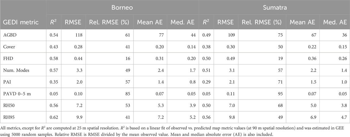
Table 3. Validation statistics for GEDI Fusion 2021 predictions using held-out GEDI observations.

We also evaluated a GEDI Fusion hindcast (2015) prediction map of vegetation height (RH95) at 90 m spatial resolution using ALS data acquired across a large portion of Borneo. The linear relationship between the GEDI Fusion prediction of RH95 and ALS vegetation height from approximately the same time is shown in Figure 3. The overall trend is close to the 1:1 line, but has considerable noise on either side. Notably, GEDI Fusion height predictions are overestimated when ALS vegetation height is low, and tend to be underestimated when ALS vegetation height is greater than about 25 m. GEDI-CCDC Fusion height predictions saturate around 35 m, consistent with the saturation of photosynthetically active radiation in the Landsat absorption bands and near infrared reflectance as canopy cover closes.

Figure 3

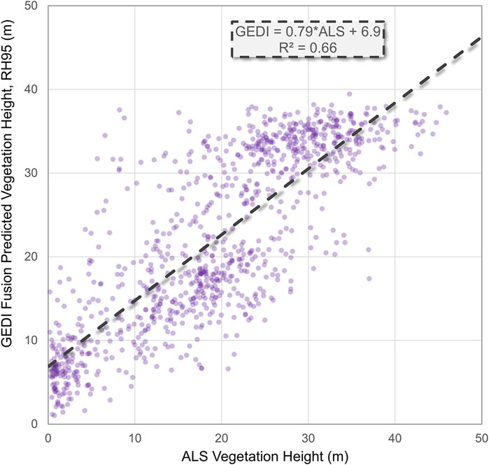
Figure 3. Comparison of GEDI Fusion predicted vegetation height (RH95) at 90 m spatial resolution vs. airborne laser scanning (ALS) vegetation height, resampled to 90 m spatial resolution. GEDI Fusion predictions correspond to the year 2015 while ALS vegetation height was measured in October 2014. The dashed line shows a linear fit and the associated equation is displayed in a dashed box.

3.2 SDM performance

For each species of interest in a region (hereafter “cases”) we ran 10 bootstraps and considered five different model scenarios, resulting in 3,250 total RF and GLM models. In terms of model performance, there are several facets to consider. First, we focus on model performance as it relates to the algorithm (RF vs. GLM) and the five different model scenarios listed in Table 2. We calculated the mean AUC from 10 bootstraps per case in order to quantify which modeling algorithm and scenario yielded meaningfully better performance, which we specify using a threshold of 0.01 AUC. When comparing the performance of the two model algorithms used, RF consistently outperformed GLM (Table 4), having a meaningfully higher mean AUC in approximately 75% of cases aggregated over both islands. With this in mind, most of the subsequently reported results focus on RF models.

Table 4

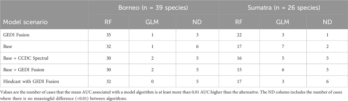
Table 4. Comparing mean AUC by model algorithm for species in Borneo and Sumatra. Comparisons are between model algorithms, separately for each region (i.e., across rows).

There are several comparisons to examine when summarizing performance by model scenario. The mean performance for all species in both regions was very similar for all model scenarios, except GEDI Fusion (Table 5). Mean AUC of the GEDI Fusion scenario was approximately 0.04 and 0.09 less for RF and GLM, respectively.

Table 5

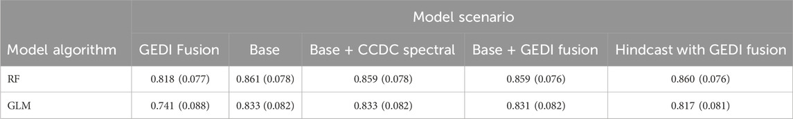
Table 5. Mean (standard deviation) model performance (AUC) for all species in both regions, grouped by model algorithm and scenario.

When examining individual species and comparing mean AUC associated with different model scenarios, there were only a few cases (species in a region) where one model scenario performed meaningfully better than others regardless of the modeling algorithm, that is the AUC of one model scenario is more than 0.01 higher than the next best performing scenario for that species and algorithm (RF in Table 6; GLM in Supplementary Table S3). Therefore there was not usually a single model scenario which clearly performs best when a large number of diverse, somewhat correlated predictors are considered.

Table 6

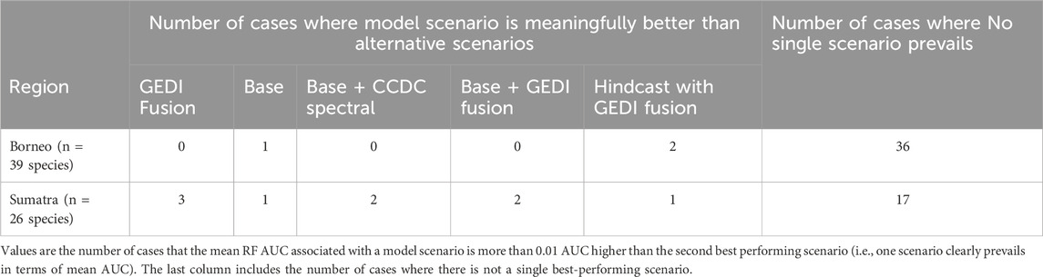
Table 6. Comparing mean RF AUC by model scenario for species in Borneo and Sumatra. Comparisons are between model scenarios (i.e., across rows) and per region.

Other interesting scenario performance comparisons to consider related to the utility of GEDI Fusion variables are 1) Base + GEDI Fusion versus Base, 2) Base + GEDI Fusion versus Base + CCDC Spectral, and 3) Hindcast with GEDI Fusion versus Base. First, with the RF model algorithm there were only 4 cases where the Base + GEDI Fusion scenario showed meaningful improvement (>0.01 AUC) relative to the Base scenario: Southern pig-tailed macaque (Borneo and Sumatra), Asiatic golden cat (Sumatra), and Binturong (Sumatra). Surprisingly, there were 10 cases where the Base scenario had meaningfully higher AUC than the corresponding Base + GEDI Fusion scenario despite the fact that Base + GEDI Fusion considers a larger pool of potential predictors. With the GLM algorithm there were only 3 cases where the Base + GEDI Fusion scenario showed meaningful improvement (>0.01 AUC) relative to the Base scenario: Bornean yellow muntjac (Borneo), Horse-tailed squirrel (Borneo), and common palm civet (Sumatra). Similar to RF, there were 11 cases where the Base scenario had meaningfully higher AUC than the corresponding Base + GEDI Fusion scenario.

For the second comparison between Base + GEDI Fusion vs. Base + CCDC Spectral with the RF model algorithm, both comparisons yielded 6 cases that had meaningfully higher AUC than the alternative scenario. With the GLM algorithm, there were 8 cases where the Base + CCDC Spectral scenario had meaningfully higher AUC than the Base + GEDI Fusion scenario, while there were 7 cases for the alternative comparison.

For the third comparison between Hindcast with GEDI Fusion and Base with the RF model algorithm, there were 9 cases where the Hindcast scenario had meaningfully higher mean AUC than the Base scenario, compared with 13 cases for the alternative comparison. With the GLM algorithm, there were only 4 cases where the Hindcast scenario had meaningfully higher mean AUC than the Base scenario, whereas there were 36 cases where the mean AUC of the Base scenario was meaningfully higher. Hence the Hindcast with GEDI Fusion scenario coupled with RF yielded similar performance relative to the Base model scenario. The same cannot be said for GLM, which very often had meaningfully higher performance when coupled with the Base model scenario.

We highlight one visualization comparing AUC of the Base, Base + GEDI Fusion, and Hindcast with GEDI Fusion model scenarios (Figure 4) per case, focusing on the RF model algorithm (see Supplementary Figure S4 for GLM). Figure 4 conveys several relevant outcomes. First, model performance was typically better for Borneo species models, relative to Sumatra species models. Furthermore, the variability of AUC was typically smaller for Borneo species models compared to Sumatra species models. Second, nearly all region and species models had good quality AUC values (>∼0.7). Depending on the scenario of interest, approximately 15 cases had excellent mean performance (>∼0.9 AUC). Third, the difference in performance between these three model scenarios was relatively small.

Figure 4

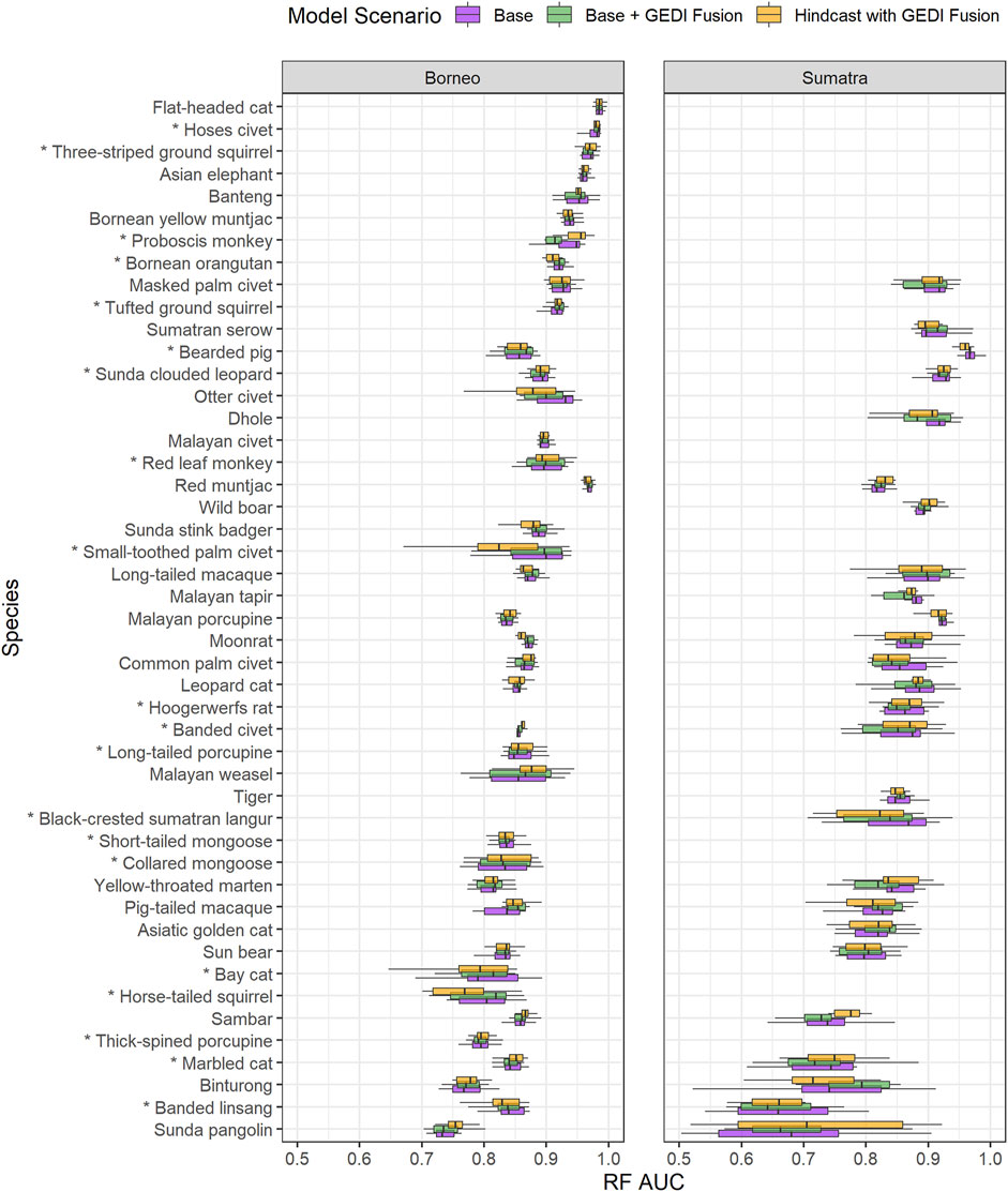
Figure 4. Boxplot summaries of AUC associated with random forest (RF) models for 10 bootstraps per region and species. The area under the curve (AUC) measures the ability of the model to distinguish between presence and absence, with higher values indicating better models. Species are ordered by mean AUC of Borneo and Sumatra models. Boxplot colors correspond to different model scenarios. Asterisks indicate that a species only has “forest” as its suitable level 1 IUCN habitat.

3.3 SDM predictor importance

We assessed predictor importance in several ways, all of which examined the permutation mean decrease in AUC. We highlight results from RF models since they performed best for the vast majority of species. First, across all cases we computed the frequency of each predictor group’s relative ranked importance (Figure 5; see Supplementary Figure S5 for GLM). For every scenario, Survey Effort (number of camera trap nights) was most frequently ranked as the top predictor. Climate or Geomorphology were the next most frequently ranked top predictors, followed by Human Influence. GEDI Fusion Structure metrics were not frequently selected or frequently ranked in the top 3 for the Base + GEDI Fusion scenario. They were more frequently selected in the Hindcast with GEDI Fusion scenario, but still not near the top of the groupwise importance rankings. CCDC Spectral Indices were more commonly selected in the Base + CCDC Spectral scenario relative to GEDI Fusion Structure metrics in the Base + GEDI Fusion scenario. The only difference between these two scenarios was the swapping of Spectral Indices and GEDI Fusion Structure metrics, which were themselves partly derived from spectral indices. In other words, when considering all cases the CCDC spectral indices are relatively more important than GEDI Fusion structure metrics when added to the Base model scenario.

Figure 5

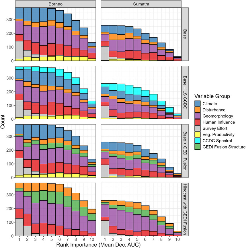
Figure 5. The frequency of each predictor group’s relative ranked importance (in terms of permutation mean decrease in AUC) across all region and species RF models for four different scenarios. A rank of 1 corresponds to the highest importance (i.e., largest mean decrease in AUC when the variable is excluded), while a rank of 10 corresponds to lowest importance. Note that only mean decrease in importance values greater than 0.001 are used for aggregating variables from the different groups. Hence there are lower counts for the higher ranks.

Second, we considered the percentage of models where at least one GEDI Fusion metric ranked in the top 5 for each case and bootstrap, considering both the Base + GEDI Fusion and Hindcast with GEDI Fusion scenarios (Figure 6). Overall, the majority of Base + GEDI Fusion species models do not include GEDI metrics ranked in the top 5, but there are several exceptions, such as the marbled cat and banded linsang. The Hindcast with GEDI Fusion scenario yields a higher percentage of GEDI Fusion metrics in the Top 5, with approximately half of the cases having at least one GEDI Fusion metric which ranks in the Top 5 for at least 50% of bootstraps.

Figure 6

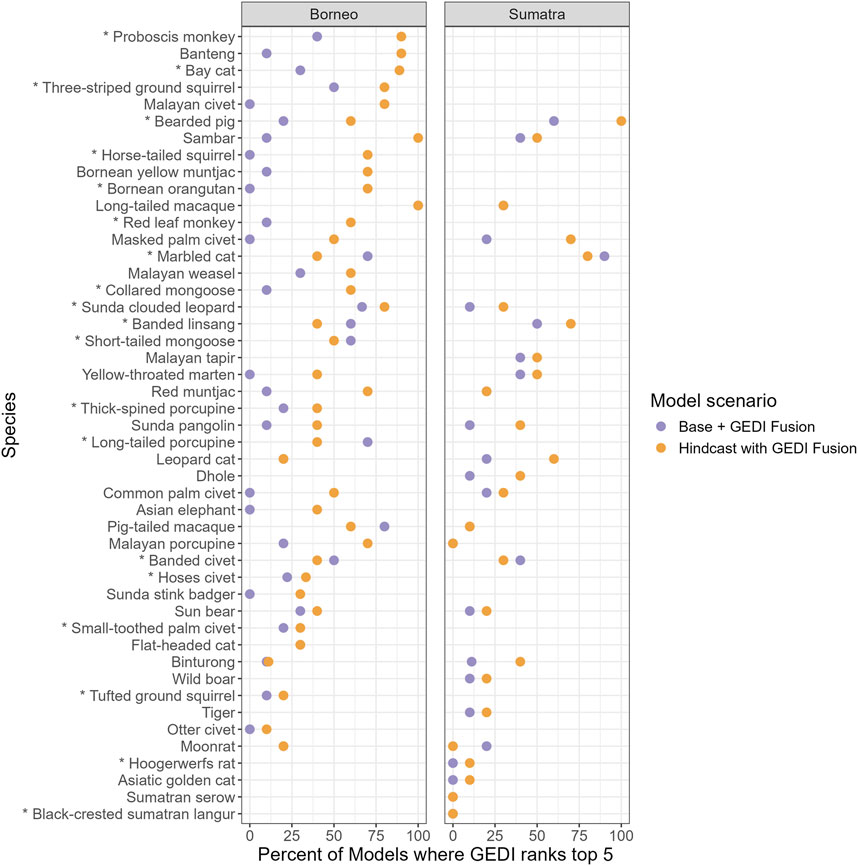
Figure 6. The percent of Base + GEDI Fusion and Hindcast with GEDI Fusion RF models (across 10 bootstraps) where at least one GEDI Fusion metric ranks in the top 5 of variable importance, computed as the permutation mean decrease in AUC. Point coloring is used to contrast scenarios. Species are ordered by the average percent of Hindcast with GEDI Fusion models where at least one GEDI Fusion metric ranks in the top 5. Asterisks indicate that a species only has “forest” as its suitable level 1 IUCN habitat.

Third, for every case we computed the permutation mean decrease in AUC for each bootstrap. We aggregated the mean decrease in AUC from each bootstrap and for each predictor group, allowing us to visualize the cumulative importance of predictor groups for each species, as well as the frequency of variable selection. An example is shown below in Figure 7 for Bearded pig. This example illustrates how the relative importance of variable groups varies across regions and model scenarios. For the Bearded pig, GEDI Fusion Structure is relatively more important in Sumatra than in Borneo. Furthermore, we see that the relative importance of GEDI Fusion Structure is noticeably higher in the Hindcast with GEDI Fusion scenario.

Figure 7

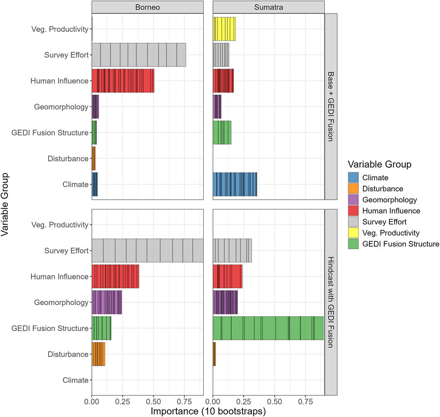
Figure 7. Bearded pig variable importance, computed as the permutation mean decrease in RF AUC, aggregated by variable group over 10 bootstraps. Each bin corresponds to a predictor associated with the specified group and the width of the bin corresponds to the mean decrease in AUC when that variable was permuted for a given bootstrap. The top set of plots corresponds to the Base + GEDI Fusion scenario, while the bottom set corresponds to the Hindcast with GEDI Fusion scenario.

3.4 SDM prediction maps

Based on our workflow, there are numerous ways to visualize predicted species distribution maps. One approach is to visualize the prediction from a single bootstrap from a particular model scenario. The individual prediction could be associated with a particular evaluation metric, like the highest AUC. Another, perhaps more representative approach for visualizing predictions, is to consider all predictions from each bootstrap in aggregate. One aggregation technique calculates the per-pixel mean of the stack of bootstrap predictions (Figure 8A). Unfortunately, this mean prediction does not have associated evaluation metrics since this would require a separate holdout set of species observations, which is not practical considering the low number of presences for many species. We also calculate the per-pixel standard deviation, and use that in conjunction with the per-pixel mean to display the coefficient of variation as an estimate of per-pixel uncertainty (Supplementary Figure S6).

Figure 8

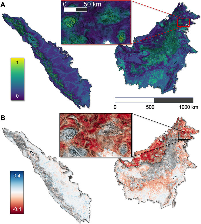
Figure 8. Sunda clouded leopard predicted probability of occurrence in 2021 (A) and change in predicted probability of occurrence from 2001 to 2021 (B). All maps correspond to the RF model algorithm with the Hindcast with GEDI Fusion model scenario. Ground slope is displayed as the basemap.

Another dimension to consider is time. The Hindcast with GEDI Fusion model scenario includes several temporally-dynamic predictor variables which are appropriate for hindcasting species’ probability of occurrence. The temporally-dynamic predictors go back to approximately the year 2001. Here we highlight the change in probability of occurrence from 2001 to 2021 for a single species with an IUCN endangered status, the Sunda Clouded Leopard (Figure 8B).

4 Discussion

4.1 Multitemporal catalog of species distributions and forest structure

Considering the necessity of forest habitat for many Sundaland mammal species and the rate of forest loss in this region, the most significant contribution of this study is the creation of a multi-temporal catalog of species distribution maps for 47 mammal species in Borneo and Sumatra, 11 of which are Endangered and 3 of which are Critically Endangered. The maps are based on an extensive camera trap network, two modeling algorithms, and the best available remotely-sensed datasets, including GEDI lidar which provides the most comprehensive tropical canopy structure metrics available to date. The combination of spatial extent, relatively-fine spatial resolution, multitemporal predictions, and number of species is unprecedented in this region as previous work has focused on distribution models of individual species or guilds (e.g., Hearn et al., 2016; Macdonald et al., 2019b; Nursamsi et al., 2023; Mendes et al., 2024; Chiaverini et al., 2023) or aggregate diversity metrics (e.g., Macdonald et al., 2020), typically at a point in time. The maps we developed and present here will be useful inputs for downstream conservation analyses and decisions. Species probability of occurrence maps can be used to evaluate the effectiveness of existing protected areas (e.g., Chiaverini et al., 2023) and identify spatial conservation priorities (Faleiro et al., 2013; Hughes, 2017; Macdonald et al., 2019a). Similar products have also been used in this region to define resistance surfaces for connectivity modeling and subsequent identification of core habitat areas (Kaszta et al., 2020). Moreover, species distribution and connectivity maps can be used to assess how previous agricultural conversion and infrastructure development projects have affected species core habitat during the Landsat period of record. Impact associated with projected development can also be assessed prior to implementation in order to inform decisions, such as relocation of the Indonesian capital (Nusantara) and the construction of major highways (e.g., Kaszta et al., 2024; Jantz et al., 2025).

The multi-temporal GEDI Fusion maps considered by each SDM are themselves an important and relatively novel contribution since multiple aspects of forest structure (beyond height and cover) have never been spatially-resolved and hindcast at the cadence used in this study. The cadence of these and other temporally-matched predictors has implications for hindcasted SDM accuracy. The GEDI Fusion predictors have a cadence of 3 years which generally is enough time to establish a new Landsat CCDC segment considering frequent cloud cover in the region. Most other predictors range from 1 to 3 years cadence, with a maximum of 5 years for the global human modification predictor (see Supplementary Table S1). The accuracy of hindcasted SDMs is related to the cadence/temporal fuzziness of temporally-matchable predictors. For example, if a particular region had few to no Landsat observations in a year, but that region experienced deforestation during that year, our prediction of GEDI forest structure metrics would have higher error, and would potentially result in a higher probability of occurrence than what would have been predicted had several Landsat observations been available for that year. Hence, considering the cadence of the predictors themselves, our hindcasted predictions should be representative of a ∼ 3–5 years time period. Change estimates should thus only be made across time periods greater than 3 years.

4.2 Utility of GEDI fusion predictors in SDMs

Another major contribution is the characterization of the utility of four-dimensional GEDI Fusion predictors in SDMs, both in terms of improving model performance and ecological inference. We compared several model scenarios (i.e., predictor sets with and without metrics representing vertical forest structure) and two algorithms for predicting the distribution of mammal species in Borneo and Sumatra. Regarding model performance, one of our key outcomes is that species models including GEDI Fusion variables do not, from a practical standpoint, perform better than alternate model scenarios. For the RF algorithm there were only 4 cases (out of 65) where the Base + GEDI Fusion scenario performed meaningfully better (AUC >0.01) than the baseline (Base) scenario. The Hindcast with GEDI Fusion scenario yielded 9 cases with meaningful increases in model performance relative to the Base scenario. Comparing Base + GEDI Fusion and Base + CCDC Spectral yielded a similar result.

In one sense, this set of results is surprising considering the gradient of forest structure in this region and the fact that many species are dependent on forest habitat. In another sense this is not surprising considering the relatively high-degree of correlation among predictors, both within the same group and across groups (Supplementary Figure S7). GEDI Fusion variables are all highly correlated between themselves and with several Climate, Disturbance, and Geomorphology variables, which is also not surprising considering elevation and forest cover loss were included in making continuous predictions of GEDI Fusion metrics, and that elevation inherently has a strong positive relationship with forest structure in this region and the tropics in general (Liu et al., 2025). As a result, the GEDI metrics may not be selected in models if they didn’t make it through the initial GVIF variable selection routine, which often selected other predictors based on preliminary training and importance scores. Moreover, a principal component analysis of our GEDI Fusion predictors resulted in only 2–3 informative components based on the Eigen value scree plot and visual analysis of PC bands. As a result, there may not be as many unique dimensions to our GEDI Fusion products as expected.

Another reason GEDI metrics might not lead to large improvements in performance is the fact that most metrics tend to saturate (or lose discrimination) where forests are tall and very dense. In the case of RH98 (canopy height), approximately half of the camera trap sites have predicted RH98 values greater than 30 m, which is around the height that saturation of RH98 predictions occurs (Figure 3). Furthermore, based on comparisons with a discontinuous 1 km gridded dataset that only used actual GEDI data in aggregate (Burns et al., 2024), we expect at least the upper 25% of RF predicted canopy height values are indiscriminate, i.e., the approximate maximum predicted canopy height is 40 m, while this value only corresponds to approximately the 75th percentile of the gridded distribution. In general we expect most RF predicted canopy heights greater than 30 m will be associated with minimally structurally-disturbed forests, so that unintentional threshold associated with saturation is somewhat ecologically relevant. But the loss of height discrimination starting somewhere between 30 and 40 m and possibly up to 70 m may be an important limitation for the prediction of some species which use very tall forests. At the same time, animals that make full use of that vertical space may also be more challenging to detect with camera traps placed close to ground level (discussed further below). PAVD from 0 to 5 m, which is the stratum where camera traps are placed, was not reliability predicted (R² = 0.05). Considering many of the species in this analysis are frequently found at ground level, PAVD from 0 to 5 m might actually be a very relevant predictor. But the reliability and lack of discrimination of this GEDI Fusion structure metric may preclude initial GVIF selection and limit model discrimination and subsequent inference.

Despite only yielding limited improvements in model performance, GEDI Fusion predictors do offer novel habitat insights for some species and arguably improve ecological interpretability of SDMs. Consider correlated predictors from two different model scenarios, Base + CCDC Spectral and Base + GEDI Fusion - NDVI and GEDI Fusion canopy height (RH98). NDVI does somewhat represent vegetation structure (or at least vegetation density), but in tall, dense forests it primarily corresponds to reflectance from the top of the canopy (Gao et al., 2023). Canopy height predicted from fusion of GEDI and Landsat CCDC is not necessarily more reliable considering the aforementioned saturation issues of NDVI (and other spectral vegetation indices) and the propagated uncertainty associated with fusion modeling (Moudrý et al., 2024), but canopy height is more interpretable for ecologists and decision makers. Even though it may be challenging to accurately measure the height of a 70 m tree from the ground, canopy height is still much more intuitive than a spectral index like NDVI. Other GEDI Fusion metrics, like PAI, FHD, or understory PAVD, may not be quite as intuitive, but three-dimensional forest structure is more tangible and closely linked to species habitat preferences compared to spectral indices which focus on canopy tops and make use of wavelengths that are beyond the perception of human vision. Thus, while incorporating GEDI Fusion metrics does not, in general, substantially improve model performance, these predictors enhance our understanding of species’ habitats for practical management and applied ecological purposes.

Supplementary Figure S8 shows the partial dependence of Sunda clouded leopard probability of occurrence considering several GEDI Fusion metrics, separated into two groups corresponding to focal mean and focal standard deviation. For this species, probability of occurrence generally increases as the focal mean of each GEDI Fusion metric increases. Probability of occurrence generally decreases as the focal standard deviation of each GEDI Fusion metric increases (i.e., forest structure surrounding a camera trap site is relatively more heterogeneous). The GEDI Fusion partial dependence plots for Sunda clouded leopard also show that metrics with focal standard deviation applied were more frequently selected than those with focal mean applied. We observed the same pattern in many of the SDMs (see additional partial dependence plots in Supplementary Material). This is not necessarily surprising considering the focal standard deviation metrics generally have a lower degree of correlation with predictors from other groups. Hence when considering Base + GEDI Fusion or Hindcast model scenarios, the GEDI Fusion focal standard deviation predictors tended to be favored (relative to focal mean) in the groupwise variance inflation factor variable selection routine. Multiscale optimization is now more commonly used in SDMs, but is usually done based on mean and rarely based on focal SD. One important implication of our study for multiscale machine learning models is that optimization on multiscale variation may be more important than optimization on multiscale mean, at least when a large pool of correlated predictors are considered.

The focal standard deviation of GEDI Fusion metrics is a relevant way to characterize the heterogeneity of forest structure in this region. Examining maps of GEDI Fusion metrics with focal standard deviation applied, low values typically correspond to homogeneous forests and high values correspond to edges, such as an undisturbed forest next to an agricultural area. Edges are known to influence forest vertebrate abundance (Pfeifer et al., 2017) and recent work utilizing GEDI showed that edge effects on interior canopy structure may extend further than previously thought, to about 1.5 km (Bourgoin et al., 2024). Although GEDI Fusion metrics are identifying prominent edges that can also be detected by optical satellites like Landsat or Sentinel-2, there is promise for characterizing actual structural edges (Nguyen et al., 2023) instead of spectral edges primarily associated with the top of the canopy. Additional texture and heterogeneity metrics (sensu Torresani et al., 2023) may represent other forest structure configurations and provide more relevant information for prediction of some species distributions.

4.3 Perspectives on SDM methodological options

There are multiple metrics and lines of evidence for choosing the “best” combination of model algorithm and scenario to use for spatial prediction and inference. Regarding model metrics, we chose to base our model assessments and comparisons on the commonly used AUC metric because it considers both sensitivity (the true presence rate) and specificity (the true absence rate) across a range of presence/absence thresholds. We were not concerned with absolute presence/absence predictions associated with the choice of a threshold, but rather the relative patterns of probability of occurrence. Nonetheless, it may be worth considering other performance metrics. Sofaer et al. (2019) showed that area under precision recall curve (related to F1 and analogous to AUC but with precision and recall instead of sensitivity and specificity) had important advantages for evaluating rare species, in particular, since true absences are not considered. However, Flach and Kull (2015) recommended plotting precision-recall curves in a different coordinate system, noting a key advantage because the area under Precision-Recall-Gain (PRG) curves yields an expected F1 score on a harmonic scale. To compare area under the receiver operator characteristic curve (AUC ROC/AUC) and AUC PRG, we focused on models for Borneo species (the region with the most data and best performing models), showing the differences between two different model scenarios and the baseline scenario per bootstrap in terms of AUC PRG (Supplementary Figure S9). We found few species had many models which used GEDI Fusion predictors that were very different from the baseline scenario. This is generally in line with our findings based on AUC ROC. Regarding the model algorithm, we found RF performed better than GLM in the vast majority of SDMs. One of the key methodological differences between modeling algorithms we used here was the decision to balance presence and absence samples for RF, but not GLM. RF has been shown to be sensitive to class imbalance (Evans and Cushman, 2009; Valavi et al., 2021) while GLM is generally thought to be less sensitive or insensitive. Future work could evaluate model performance using independent validation data and compare effects of different class imbalance ratios across these combinations of modeling approaches.

The Hindcast with GEDI Fusion model scenario, while not always the best performing, is an attractive option to focus on for several reasons. First, it is relatively parsimonious since it only considers predictors which are either relatively fine spatial resolution or temporally-resolved. Intuitively, this composition of predictors is appropriate for such a dynamic landscape. While most patterns of species occurrence will be correlated to some degree with coarse resolution climate predictors (e.g., mean annual temperature or precipitation), changes in climate are not thought to be the primary factors driving changes in mammal species occurrence over the last few decades in this region (Jaureguiberry et al., 2022). Moreover, several predictor groups, such as CHELSA Bioclim and SoilGrids, are themselves modeled using topography predictors, and hence the groups are often highly correlated. Therefore, including high spatial and/or temporal resolution geomorphology predictors, which may themselves be proxies for climate or soil properties, permits finer spatial resolution predictions. Fine resolution human influence and forest structure predictors are other obvious sets of predictors to include in this model scenario, since a large portion of the landscape is affected by conversion to palm oil plantations (Descals et al., 2021) and hunting pressure (Deith and Brodie, 2020).

For the majority of species models, there is no meaningful difference in model performance between the Hindcast with GEDI Fusion and Base (or Base + GEDI Fusion) model scenarios (Figure 4). However the key difference is how we interpret the importance of predictors in these different scenarios. GEDI Fusion forest structure predictors are used more often in the Hindcast with GEDI Fusion scenario relative to the Base + GEDI Fusion scenario (Figures 5–7). In general, the GEDI Fusion structure predictors are taking the place of Vegetation Productivity and Climate predictors, which is relevant because these groups of predictors are correlated. Similarly, Wilson et al. (2013) found a surprisingly weak contribution of forest structure in St. Francis’ satyr butterfly distribution models, suggesting undetected correlations with other variables (terrain, land cover) reduced predictive power. The other comparison to highlight in Figure 5 is the use of spectral indices in the Base + Landsat CCDC scenario, relative to structure predictors in the Base + GEDI Fusion scenario. Spectral indices are relatively more important than GEDI Fusion forest structure predictors. From a signal-to-noise perspective, this is not surprising since the spectral indices are closer to the original sensor observation and have been aggregated temporally using the CCDC algorithm. In contrast, GEDI Fusion structure metrics predicted from Landsat CCDC include relatively more noise due to factors like GEDI geolocation uncertainty and saturation of spectral indices (e.g., NDVI) in more dense forests.

Given the relatively high degree of correlation among GEDI Fusion metrics and between GEDI Fusion metrics and other predictor groups, it is worth considering alternate methods for generating continuous maps of vegetation structure to use as inputs in SDMs. One alternate method is statistical aggregation (i.e., gridding) of GEDI shots within a practical and meaningful pixel size. For vegetation structure, a statistically meaningful pixel size would be on the order of 1 km, ideally finer. Dubayah et al. (2021b) and Burns et al. (2024) have produced gridded products in this manner, but unfortunately large gaps in GEDI quality-shot coverage in the tropics yield large gaps in the gridded maps at 1 km spatial resolution, which is problematic for making continuous predictions of species probability of occurrence (and why we did not utilize these products in this study). A second option is geostatistical interpolation, such as kriging. We developed a set of GEDI predictors which were kriged at 1 km spatial resolution (Brodie et al., 2023) and considered using these kriged GEDI structure metrics since this method usually improves the prediction of low and high values in dense forests relative to fusion with Landsat CCDC. Unfortunately, there are still many large gaps in GEDI coverage in the tropics which require interpolating over large distances. This is problematic since, for example, forest structure is locally variable as a function of topography, human influence and other factors. Therefore, while exploratory models combining the Base set of predictors and Kriged GEDI metrics had performance on par with Base + GEDI Fusion models, the former models had more problematic spatial artifacts associated with the kriging interpolation. Ultimately, even though GEDI Fusion predictors did not capture high structure values as well as hoped, we preferred them over GEDI Kriged predictors since they had a finer spatial resolution, fewer spatial artifacts, and could be used for hindcasting.

The model scenarios we used were designed to include a multitude of factors known to influence species habitat. We sought to create a semi-automated SDM pipeline, and considering the large number of species and uncertainty regarding the habitat preferences of some species, we used an automated variable selection approach. This choice impacted how often GEDI Fusion metrics were selected and the resulting interpretation of variable importance. This data-driven approach has merits, including automation and potential to gain novel insights about the habitat preferences of understudied species. Nonetheless, it would also be beneficial to include expert knowledge in the variable selection process, especially since models (especially RF) tended to optimize performance regardless of model scenario (excluding the scenario which only used GEDI Fusion predictors). Previous studies have advocated for expert input in SDMs (Petitpierre et al., 2017; Fourcade et al., 2018), but this requires a greater level of coordination and collaboration across disciplines (e.g., Velásquez-Tibatá et al., 2019). Remote sensing scientists and ecological modelers can certainly learn from biologists who study these species in the field, while biologists can also gain insights from the exploration and incorporation of novel geospatial datasets.

4.4 Species monitoring limitations

While one of the primary components of this study is assessing the utility of remotely-sensed forest structure metrics in SDMs, it is also important to note other considerations associated with the species survey design. Estimating presence/absence from camera trap observations is an imperfect process (Zwerts et al., 2021). Here we used a relatively low number of camera trap nights (30) to designate the absence of a species at a site. For most species, we found the number of camera trap nights to be the most important predictor of species probability of occurrence - more nights typically meant a higher probability of detection occurrence. Future work may consider other ways of incorporating survey effort information in the context of absences, possibly by using the number of camera trap nights as case weights in RF and GLM models. Higher case weights would correspond to more camera trap nights (i.e., higher likelihood of true absence), and the higher weighted observations would be used more often in the model fitting process, potentially improving discrimination between presences and absences.

In a dense forest many of the species we modeled are inherently challenging to detect with camera traps since they may be obscured by vegetation. Hence, areas with more open understories (i.e., lower PAVD from 0 to 5 m) may appear to have more species occurrences, relative to very dense understories. However, this might not align with the species’ actual habitat preferences, largely due to detectability. Unfortunately this conundrum is difficult to resolve with our current GEDI Fusion products since PAVD from 0 to 5 m was the most challenging forest structure metric to predict (R² = 0.05 and Rel. RMSE = 85–95%). Detection with camera traps is even more challenging for primarily arboreal species that spend little time on the ground within the view of most camera traps. Therefore it is likely that arboreal mammal presences are underestimated, leading to model predictions that are biased towards absence. For RF models, our use of balanced presence and absence sample sizes (i.e., down-sampling) per decision tree may have partially reduced this bias, but the tradeoff of down-sampling is that some (typically absence) locations will not be considered in an individual bootstrap model. Research teams have already taken the obvious next steps of tracking arboreal species with GPS (McLean et al., 2016) and deploying camera traps in the upper canopy to observe scansorial and arboreal species (Haysom et al., 2021; Honda et al., 2025). Acoustic recording units (ARU), possibly coupled with camera traps (Garland et al., 2020), could provide another complementary piece of occurrence information, especially when vegetation is very dense. In the case of either technology (camera trap or ARU), the influence of vegetation density on species detection would need to be considered. Emerging technologies, such as tracking tagged animal movement via micro transmitters detected by small satellites (Cube Sats) has the potential to rapidly advance our understanding of habitat use, resource selection and migration routes.

4.5 Moving forward with spaceborne lidar in biodiversity analyses

Our results should not be taken to imply that forest structure per se is not a strong predictor of mammal species probability of occurrence, but rather that the GEDI Fusion predictors do not substantially improve prediction in this region relative to a baseline model scenario, which included co-varying predictors of climate, geomorphology, disturbance, human influence and vegetation productivity spanning local to landscape scales. Previous studies have demonstrated the utility of high-resolution vegetation structure from ALS for modeling species habitat associations in this region (Davies et al., 2017; Deere et al., 2020). Future work using higher density and/or quality remotely sensed forest structure data may find substantially different results, particularly in hierarchical frameworks which explicitly consider different levels (scales) of landscape structure (e.g., Nursamsi et al., 2023) and connectivity. In our analysis, the utility of GEDI Fusion forest structure metrics in terms of performance was limited for three main reasons: 1) predictions of the tallest forests (30 + m) and understory PAVD from 0 to 5 m were unreliable, 2) there was a high degree of correlation between GEDI Fusion predictors and limited effective dimensionality, and 3) there was a high degree of correlation between GEDI Fusion predictors and geomorphology predictors, in particular, making it challenging to disentangle their unique impacts on model performance. However, in terms of model inference, GEDI Fusion predictors are a step in the right direction, offering habitat insights and improved ecological interpretability.

Moving forward, we expect forest structure metrics derived from GEDI, and ultimately next-generation spaceborne lidar missions designed for terrestrial ecological applications, to have greater utility in SDMs for several reasons. First, after a brief ∼1 year hibernation period from March 2023 to April 2024, GEDI began reacquiring data. Data coverage will improve with time on-orbit which will likewise improve continuous structure maps generated using gridding, kriging, or fusion with image data. Moreover, GEDI data accuracy and quality are expected to improve in future versions of the data products. For example, horizontal geolocation uncertainty is expected to decrease to about 5 m for data release 4. Unfortunately, the tropics, which harbor the bulk of the world’s terrestrial species and above ground carbon, will continue to have relatively less GEDI coverage than higher latitudes due to ISS orbital geometry and greater cloud cover over dense humid forests. Hence, fusion strategies will continue to be a necessary bridge for creating fine spatial resolution, continuous forest structure predictors until new satellite instruments and/or constellations with improved spatial and temporal coverage are operational. Fortunately from the bridge perspective, many new satellite missions and datasets which could be fused with GEDI are already online or coming online soon. For example, Planet Labs 3 m imagery will be helpful for better characterizing vegetation texture/heterogeneity while also providing phenological context in fusion models. The NASA-ISRO SAR mission (NISAR) will use L-band (∼23 cm wavelength) measurements capable of penetrating into forest canopies. The L-band backscatter measurement is closely correlated with forest structure, particularly when calibrated with LiDAR measurements, since the transmitted wavelength interacts with stems and branches.

Novel and emerging deep learning models should also be explored for making spatio-temporal predictions of forest structure metrics and species distributions. Regarding forest structure, several studies focused on this region have demonstrated the capability of using deep learning for mapping oil palm plantations (Descals et al., 2021; Rodriguez et al., 2021), which are a major driver of deforestation and habitat loss (Hughes, 2017). In terms of GEDI-measured forest structure, multiple studies have reported improved performance when applying deep learning models trained on satellite imagery (Lang et al., 2023; Schwartz et al., 2023; Wagner et al., 2024) since these models are able to learn complex features across spatial and temporal scales. In regards to species distribution models, convolutional neural networks (CNN) are appealing because they leverage the spatial context (i.e., texture) of environmental predictors (Brodrick et al., 2019). For example, Deneu et al. (2021) found local landscape structure improved the predictive performance of CNN-SDMs and that this modeling framework outperformed RF when evaluated by mean top-k accuracy, but not AUC and TSS. In this study we applied simple convolutions (gaussian focal mean and standard deviation) to predictor variables. Notably, we found the focal SD of some GEDI metrics, a proxy for forest structure heterogeneity and a way to identify edges, to be relatively important for certain species distributions. We used a relatively small number of multiscale convolutions relative to current CNN architectures, so additional performance gains may be possible with more numerous and complex convolutions in a CNN framework. Lastly, the availability of massive pre-trained foundational models, especially those tailored to multispectral and multiscale datasets (e.g., SpectralGPT, Hong et al., 2024), may increase model efficiency and performance.

Our results are encouraging in terms of model performance and advancing interpretation of animal habitat use by incorporating forest structure metrics that are more tangible relative to other predictors, such as vegetation spectral indices. Given the extreme rapidity of forest loss in many tropical regions and expected impacts related to economic expansion in Sundaland (e.g., Nusantara), having a catalog of 47 species models that are able to be hindcasted across decades (in this case from 2001 to 2021) and updated into the future is extremely valuable for conservation purposes (e.g., Shirk et al., 2023). This catalog will enable a multi-temporal assessment of changes in the habitat extent, pattern, and connectivity for a broad swath of Sundaland mammal biodiversity, assessment of protected area effectiveness, identification of unprotected areas of high biodiversity value, and projection of likely future changes to multi-species habitat quality and extent.

Data availability statement

Given the extremely sensitive nature of species occurrence data with respect to illegal wildlife trade, locations of camera traps will not be made public at this time to avoid further endangering the already threatened species. However, we welcome correspondence with scholars and conservationists regarding collaborative use of the data to advance science and conservation of SE Asian mammal species. All prediction maps (90 m GeoTIFF files) for years 2001 and 2021, with the exception of those for critically endangered species, are publicly available in a Zenodo repository (https://zenodo.org/records/15231415). Prediction maps for critically endangered species will be curated by the relevant IUCN taxonomic authority (i.e., specialist group) and may be made available upon request. Code is available in a github repository (https://github.com/burnspat/sunda_sdm_gedi).

Author contributions

PB: Conceptualization, Data curation, Formal Analysis, Funding acquisition, Investigation, Methodology, Project administration, Software, Supervision, Validation, Visualization, Writing – original draft, Writing – review and editing. ZK: Conceptualization, Funding acquisition, Investigation, Methodology, Project administration, Writing – original draft, Writing – review and editing, Data curation, Formal Analysis, Software, Validation, Visualization. SC: Conceptualization, Data curation, Formal Analysis, Funding acquisition, Investigation, Methodology, Software, Validation, Visualization, Writing – original draft, Writing – review and editing. JB: Conceptualization, Investigation, Methodology, Writing – original draft, Writing – review and editing, Data curation, Software. CH: Investigation, Methodology, Writing – review and editing, Formal Analysis, Software. PJ: Conceptualization, Funding acquisition, Investigation, Methodology, Project administration, Resources, Writing – review and editing, Data curation, Software. MD: Methodology, Writing – review and editing, Data curation. ML: Methodology, Writing – review and editing, Data curation. JB: Investigation, Methodology, Writing – review and editing, Data curation. JM-A: Data curation, Writing – review and editing. DB: Writing – review and editing, Data curation. SC: Data curation, Writing – review and editing. IH: Data curation, Writing – review and editing. AH: Data curation, Writing – review and editing. ES: Data curation, Writing – review and editing. PW: Data curation, Writing – review and editing. DM: Conceptualization, Data curation, Funding acquisition, Project administration, Supervision, Writing – review and editing. SG: Conceptualization, Funding acquisition, Investigation, Methodology, Project administration, Resources, Supervision, Writing – original draft, Writing – review and editing.

Funding

The author(s) declare that financial support was received for the research and/or publication of this article. Funding was provided by NASA Earth Ventures grant NNL15AA03C and NASA Terrestrial Ecology grant 80NSSC21K0189 to SG. The WildCRU fieldwork and staff were largely funded by a programmatic grant to DWM from the Robertson Foundation and grants from Panthera. MSL was supported by an Australian Research Council Discovery Early Career Researcher Award #DE21010.

Acknowledgments

Some of the data used here came from long-term research in Sabah supported by the Southeast Asian Rainforest Research Partnership, the Sabah Forestry Department, Sabah Parks, Sabah Wildlife Department, Yayasan Sabah, and the United Nations Development Programme. We are grateful to the many field assistants and collaborators who helped with the data collection, particularly S.W. Teoh. Additional data used in this analysis come from more than a decade-long camera-trapping study of clouded leopards and associated biodiversity. We gratefully acknowledge the hard work of the WildCRU field assistants who helped us in each study area, and the various authorities that approved WildCRU’s work. In particular, we thank the past and present leaders of WildCRU field teams, and our collaborators on the Sunda Islands: Dr Matt Linkie (WCS Indonesia), Dr. Ewan Macdonald (Worcester College, University of Oxford), Ms Jo Ross (WildCRU), Mr Gilmoore Bolongon. The acknowledgements for data contributed by the Ecological Cascades Lab and in-country collaborators are listed in Decœur et al. (2023) and Mendes et al. (2024). The Advanced Research Computing team at Northern Arizona University provided high performance computing support. Google Earth Engine has been an invaluable tool for our work. In addition to providing a consolidated public data catalog and free computing resources, we benefited from additional storage, as well as training and networking at Geo For Good Summits. The NASA GEDI Science Team provided helpful guidance regarding GEDI data processing.

Conflict of interest

The authors declare that the research was conducted in the absence of any commercial or financial relationships that could be construed as a potential conflict of interest.

Generative AI statement

The author(s) declare that no Gen AI was used in the creation of this manuscript.

Publisher’s note

All claims expressed in this article are solely those of the authors and do not necessarily represent those of their affiliated organizations, or those of the publisher, the editors and the reviewers. Any product that may be evaluated in this article, or claim that may be made by its manufacturer, is not guaranteed or endorsed by the publisher.

Supplementary material

The Supplementary Material for this article can be found online at: https://www.frontiersin.org/articles/10.3389/frsen.2025.1563430/full#supplementary-material

References

Amatulli, G., McInerney, D., Sethi, T., Strobl, P., and Domisch, S. (2020). Geomorpho90m, empirical evaluation and accuracy assessment of global high-resolution geomorphometric layers. Sci. Data 7 (1), 162. doi:10.1038/s41597-020-0479-6

PubMed Abstract | CrossRef Full Text | Google Scholar

Amir, Z., Moore, J. H., Negret, P. J., and Luskin, M. S. (2022). Megafauna extinctions produce idiosyncratic Anthropocene assemblages. Sci. Adv. 8 (42), eabq2307. doi:10.1126/sciadv.abq2307

PubMed Abstract | CrossRef Full Text | Google Scholar

Barbet-Massin, M., Jiguet, F., Albert, C. H., and Thuiller, W. (2012). Selecting pseudo-absences for species distribution models: how, where and how many? Methods Ecol. Evol. 3 (2), 327–338. doi:10.1111/j.2041-210X.2011.00172.x

CrossRef Full Text | Google Scholar

Bell, D. M., Gregory, M. J., and Yang, Z. (2024). Hindcasting and updating Landsat-based forest structure mapping across years to support forest management and planning. For. Ecol. Manag. 572, 122239. doi:10.1016/j.foreco.2024.122239

CrossRef Full Text | Google Scholar

Benkendorf, D. J., Schwartz, S. D., Cutler, D. R., and Hawkins, C. P. (2023). Correcting for the effects of class imbalance improves the performance of machine-learning based species distribution models. Ecol. Model. 483, 110414. doi:10.1016/j.ecolmodel.2023.110414

CrossRef Full Text | Google Scholar

Betts, M. G., Yang, Z., Hadley, A. S., Smith, A. C., Rousseau, J. S., Northrup, J. M., et al. (2022). Forest degradation drives widespread avian habitat and population declines. Nat. Ecol. and Evol. 6 (6), 709–719. doi:10.1038/s41559-022-01737-8

PubMed Abstract | CrossRef Full Text | Google Scholar

Bourgoin, C., Ceccherini, G., Girardello, M., Vancutsem, C., Avitabile, V., Beck, P. S. A., et al. (2024). Human degradation of tropical moist forests is greater than previously estimated. Nature 631 (8021), 570–576. doi:10.1038/s41586-024-07629-0

PubMed Abstract | CrossRef Full Text | Google Scholar

Breiman, L. (2001). Random forests. Mach. Learn. 45 (1), 5–32. doi:10.1023/A:1010933404324

CrossRef Full Text | Google Scholar

Brodie, J. F., Giordano, A. J., Zipkin, E. F., Bernard, H., Mohd-Azlan, J., and Ambu, L. (2015). Correlation and persistence of hunting and logging impacts on tropical rainforest mammals. Conserv. Biol. 29 (1), 110–121. doi:10.1111/cobi.12389

PubMed Abstract | CrossRef Full Text | Google Scholar

Brodie, J. F., Mohd-Azlan, J., Chen, C., Wearn, O. R., Deith, M. C. M., Ball, J. G. C., et al. (2023). Landscape-scale benefits of protected areas for tropical biodiversity. Nature 620 (7975), 807–812. doi:10.1038/s41586-023-06410-z

PubMed Abstract | CrossRef Full Text | Google Scholar

Brodie, J. F., Mohd-Azlan, J., and Schnell, J. K. (2016). How individual links affect network stability in a large-scale, heterogeneous metacommunity. Ecology 97 (7), 1658–1667. doi:10.1890/15-1613.1

PubMed Abstract | CrossRef Full Text | Google Scholar

Brodie, J. F., Strimas-Mackey, M., Mohd-Azlan, J., Granados, A., Bernard, H., Giordano, A. J., et al. (2017). Lowland biotic attrition revisited: body size and variation among climate change “winners” and “losers”. Proc. R. Soc. B Biol. Sci. 284 (1847), 20162335. doi:10.1098/rspb.2016.2335

PubMed Abstract | CrossRef Full Text | Google Scholar

Brodrick, P. G., Davies, A. B., and Asner, G. P. (2019). Uncovering ecological patterns with convolutional neural networks. Trends in ecology & evolution, 34(8), pp.734–745.

PubMed Abstract | CrossRef Full Text | Google Scholar

Burns, P., Clark, M., Salas, L., Hancock, S., Leland, D., Jantz, P., et al. (2020). Incorporating canopy structure from simulated GEDI lidar into bird species distribution models. Environ. Res. Lett. 15 (9), 095002. doi:10.1088/1748-9326/ab80ee

CrossRef Full Text | Google Scholar

Burns, P., Hakkenberg, C. R., and Goetz, S. J. (2024). Multi-resolution gridded maps of vegetation structure from GEDI. Sci. Data 11 (1), 881. doi:10.1038/s41597-024-03668-4

PubMed Abstract | CrossRef Full Text | Google Scholar

Chen, J., and Gao, M. (2021). ‘Global 1 km × 1 km gridded revised real gross domestic product and electricity consumption during 1992-2019 based on calibrated nighttime light data’. doi:10.6084/m9.figshare.17004523.v1

CrossRef Full Text | Google Scholar

Chiaverini, L., Macdonald, D. W., Bothwell, H. M., Hearn, A. J., Cheyne, S. M., Haidir, I., et al. (2022). Multi-scale, multivariate community models improve designation of biodiversity hotspots in the Sunda Islands. Anim. Conserv. 25 (5), 660–679. doi:10.1111/acv.12771

CrossRef Full Text | Google Scholar

Chiaverini, L., Macdonald, D. W., Hearn, A. J., Kaszta, Ż., Ash, E., Bothwell, H. M., et al. (2023). Not seeing the forest for the trees: generalised linear model out-performs random forest in species distribution modelling for Southeast Asian felids. Ecol. Inf. 75, 102026. doi:10.1016/j.ecoinf.2023.102026

CrossRef Full Text | Google Scholar

Crego, R. D., Fennessy, J., Brown, M. B., Connette, G., Stacy-Dawes, J., Masiaine, S., et al. (2024). Combining species distribution models and moderate resolution satellite information to guide conservation programs for reticulated giraffe. Anim. Conserv. 27 (2), 160–170. doi:10.1111/acv.12894

CrossRef Full Text | Google Scholar

Crego, R. D., Masolele, M. M., Connette, G., and Stabach, J. A. (2021). Enhancing animal movement analyses: spatiotemporal matching of animal positions with remotely sensed data using Google earth engine and R. Remote Sens. 13 (20), 4154. doi:10.3390/rs13204154

CrossRef Full Text | Google Scholar

Davies, A. B., Ancrenaz, M., Oram, F., and Asner, G. P. (2017). Canopy structure drives orangutan habitat selection in disturbed Bornean forests. Proc. Natl. Acad. Sci. 114 (31), 8307–8312. doi:10.1073/pnas.1706780114

PubMed Abstract | CrossRef Full Text | Google Scholar

Davies, A. B., and Asner, G. P. (2014). Advances in animal ecology from 3D-LiDAR ecosystem mapping. Trends Ecol. and Evol. 29 (12), 681–691. doi:10.1016/j.tree.2014.10.005

PubMed Abstract | CrossRef Full Text | Google Scholar

Decœur, H., Amir, Z., Mendes, C. P., Moore, J. H., and Luskin, M. S. (2023). Mid-sized felids threatened by habitat degradation in Southeast Asia. Biol. Conserv. 283, 110103. doi:10.1016/j.biocon.2023.110103

CrossRef Full Text | Google Scholar

Deere, N. J., Guillera-Arroita, G., Swinfield, T., Milodowski, D. T., Coomes, D. A., Bernard, H., et al. (2020). Maximizing the value of forest restoration for tropical mammals by detecting three-dimensional habitat associations. Proc. Natl. Acad. Sci. 117 (42), 26254–26262. doi:10.1073/pnas.2001823117

PubMed Abstract | CrossRef Full Text | Google Scholar

Deith, M. C. M., and Brodie, J. F. (2020). Predicting defaunation: accurately mapping bushmeat hunting pressure over large areas. Proc. R. Soc. B Biol. Sci. 287 (1922), 20192677. doi:10.1098/rspb.2019.2677

PubMed Abstract | CrossRef Full Text | Google Scholar

De Jay, N., Papillon-Cavanagh, S., Olsen, C., El-Hachem, N., Bontempi, G., and Haibe-Kains, B. (2013). mRMRe: an R package for parallelized mRMR ensemble feature selection. Bioinformatics 29 (18), 2365–2368. doi:10.1093/bioinformatics/btt383

PubMed Abstract | CrossRef Full Text | Google Scholar

Deneu, B., Servajean, M., Bonnet, P., Botella, C., Munoz, F., and Joly, A. (2021). Convolutional neural networks improve species distribution modelling by capturing the spatial structure of the environment. PLoS computational biology, 17(4), p.e1008856.

PubMed Abstract | CrossRef Full Text | Google Scholar

Descals, A., Wich, S., Meijaard, E., Gaveau, D. L. A., Peedell, S., and Szantoi, Z. (2021). High-resolution global map of smallholder and industrial closed-canopy oil palm plantations. Earth Syst. Sci. Data 13 (3), 1211–1231. doi:10.5194/essd-13-1211-2021

CrossRef Full Text | Google Scholar

Dormann, C. F., Schymanski, S. J., Cabral, J., Chuine, I., Graham, C., Hartig, F., et al. (2012). Correlation and process in species distribution models: bridging a dichotomy. J. Biogeogr. 39 (12), 2119–2131. doi:10.1111/j.1365-2699.2011.02659.x

CrossRef Full Text | Google Scholar

Dubayah, R., Blair, J. B., Goetz, S., Fatoyinbo, L., Hansen, M., Healey, S., et al. (2020). The global ecosystem dynamics investigation: high-resolution laser ranging of the earth’s forests and topography. Sci. Remote Sens. 1, 100002. doi:10.1016/j.srs.2020.100002

CrossRef Full Text | Google Scholar

Dubayah, R., Hofton, M., Blair, J., Armston, J., Tang, H., and Luthcke, S. (2021). ‘GEDI L2A elevation and height metrics data global footprint level V002’. doi:10.5067/GEDI/GEDI02_A.002

CrossRef Full Text | Google Scholar

Dubayah, R., Luthcke, S., Blair, J., Hofton, M., Armston, J., and Tang, H. (2021a). ‘GEDI L1B geolocated waveform data global footprint level V002’. doi:10.5067/GEDI/GEDI01_B.002

CrossRef Full Text | Google Scholar

Dubayah, R. O., Luthcke, S. B., Sabaka, T. J., Nicholas, J. B., Preaux, S., and Hofton, M. A. (2021b). “GEDI L3 gridded land surface metrics, version 2,”. ORNL Distributed Active Archive Center. Oak Ridge, Tennessee doi:10.3334/ORNLDAAC/1952

CrossRef Full Text | Google Scholar

Elith, J., and Leathwick, J. R. (2009). Species distribution models: ecological explanation and prediction across space and time. Annu. Rev. Ecol. Evol. Syst. 40, 677–697. doi:10.1146/annurev.ecolsys.110308.120159

CrossRef Full Text | Google Scholar

Evans, J. S., and Cushman, S. A. (2009). Gradient modeling of conifer species using random forests. Landsc. Ecol. 24 (5), 673–683. doi:10.1007/s10980-009-9341-0

CrossRef Full Text | Google Scholar

Faleiro, F. V., Machado, R. B., and Loyola, R. D. (2013). Defining spatial conservation priorities in the face of land-use and climate change. Biological Conservation, 158, 248–257.

CrossRef Full Text | Google Scholar

Flach, P., and Kull, M. (2015). “Precision-recall-gain curves: PR analysis done right,” in Advances in Neural Information Processing Systems. Editors C. Cortes, N. D. Lawrence, D. D. Lee, M. Sugiyama, and R. Garnett 1, 838–846. (Massachusetts Institute of Technology (MIT) Press). Available online at: https://papers.nips.cc/paper/5867-precision-recall-gain-curves-pr-analysis-done-right.

Google Scholar

Fourcade, Y., Besnard, A. G., and Secondi, J. (2018). Paintings predict the distribution of species, or the challenge of selecting environmental predictors and evaluation statistics. Glob. Ecol. Biogeogr. 27 (2), 245–256. doi:10.1111/geb.12684

CrossRef Full Text | Google Scholar

Gao, S., Zhong, R., Yan, K., Ma, X., Chen, X., Pu, J., et al. (2023). Evaluating the saturation effect of vegetation indices in forests using 3D radiative transfer simulations and satellite observations. Remote Sens. Environ. 295, 113665. doi:10.1016/j.rse.2023.113665

CrossRef Full Text | Google Scholar

Garland, L., Crosby, A., Hedley, R., Boutin, S., and Bayne, E. (2020). Acoustic vs. photographic monitoring of gray wolves (Canis lupus): a methodological comparison of two passive monitoring techniques. Can. J. Zoology 98 (3), 219–228. doi:10.1139/cjz-2019-0081

CrossRef Full Text | Google Scholar

Gorelick, N., Hancher, M., Dixon, M., Ilyushchenko, S., Thau, D., and Moore, R. (2017). Google earth engine: planetary-scale geospatial analysis for everyone. Remote Sens. Environ. 202, 18–27. doi:10.1016/j.rse.2017.06.031

CrossRef Full Text | Google Scholar

Greenwell, B. M., and Boehmke, B. C. (2020). Variable importance plots—an introduction to the vip package. R J. 12 (1), 343–366. doi:10.32614/rj-2020-013

CrossRef Full Text | Google Scholar

Hansen, M. C., Potapov, P. V., Moore, R., Hancher, M., Turubanova, S. A., Tyukavina, A., et al. (2013). High-resolution global maps of 21st-century forest cover change. Science 342 (6160), 850–853. doi:10.1126/science.1244693

PubMed Abstract | CrossRef Full Text | Google Scholar

Hardwick, S. R., Toumi, R., Pfeifer, M., Turner, E. C., Nilus, R., and Ewers, R. M. (2015). The relationship between leaf area index and microclimate in tropical forest and oil palm plantation: forest disturbance drives changes in microclimate. Agric. For. Meteorology 201, 187–195. doi:10.1016/j.agrformet.2014.11.010

PubMed Abstract | CrossRef Full Text | Google Scholar

Haysom, J. K., Deere, N. J., Wearn, O. R., Mahyudin, A., Jami, J., Reynolds, G., et al. (2021). Life in the canopy: using camera-traps to inventory arboreal rainforest mammals in Borneo. Front. For. Glob. Change 4. doi:10.3389/ffgc.2021.673071

CrossRef Full Text | Google Scholar

He, K. S., Bradley, B. A., Cord, A. F., Rocchini, D., Tuanmu, M.-N., Schmidtlein, S., et al. (2015). Will remote sensing shape the next generation of species distribution models? Remote Sens. Ecol. Conservation 1 (1), 4–18. doi:10.1002/rse2.7

CrossRef Full Text | Google Scholar

Hearn, A., Ross, J., Macdonald, D., Bolongon, G., Cheyne, S., Mohamed, A., et al. (2016). Predicted distribution of the Sunda clouded leopard Neofelis diardi (Mammalia: Carnivora: Felidae) on Borneo. Raffles Bulletin of Zoology, 2016(S33)

Google Scholar

Hearn, A. J., Cushman, S. A., Goossens, B., Macdonald, E., Ross, J., Hunter, L. T. B., et al. (2018). Evaluating scenarios of landscape change for Sunda clouded leopard connectivity in a human dominated landscape. Biol. Conserv. 222, 232–240. doi:10.1016/j.biocon.2018.04.016

CrossRef Full Text | Google Scholar

Hearn, A. J., Cushman, S. A., Goossens, B., Ross, J., Macdonald, E. A., Hunter, L. T. B., et al. (2019). Predicting connectivity, population size and genetic diversity of Sunda clouded leopards across Sabah, Borneo. Landsc. Ecol. 34 (2), 275–290. doi:10.1007/s10980-018-0758-1

CrossRef Full Text | Google Scholar

Honda, A., Amir, Z., Mendes, C. P., Moore, J. H., and Luskin, M. S. (2024). Binturong ecology and conservation in pristine, fragmented and degraded tropical forests. Oryx 58 (2), 218–227. doi:10.1017/S0030605322001491

CrossRef Full Text | Google Scholar

Honda, A., Beirne, C., Huarcaya, R. P., Mullisaca, F. P., Quispe, C. Q., Quispe, R. V., et al. (2025). Arboreal camera trapping reveals diel-vertical migrations in arboreal wildlife of the Peruvian Amazon rainforest. Environ. Res. Ecol. 4 (2), 025003. doi:10.1088/2752-664x/adb850

CrossRef Full Text | Google Scholar

Hong, D., Zhang, B., Li, X., Li, Y., Li, C., Yao, J., et al. (2024). SpectralGPT: Spectral remote sensing foundation model. IEEE Transactions on Pattern Analysis and Machine Intelligence.

Google Scholar

Hughes, A. C. (2017). Understanding the drivers of S outheast A sian biodiversity loss. Ecosphere 8 (1), e01624. doi:10.1002/ecs2.1624

CrossRef Full Text | Google Scholar

IUCN (2024). The IUCN red list of threatened species. Available online at: https://www.iucnredlist.org (Accessed October 1, 2024).

Google Scholar

Jaureguiberry, P., Titeux, N., Wiemers, M., Bowler, D. E., Coscieme, L., Golden, A. S., et al. (2022). The direct drivers of recent global anthropogenic biodiversity loss. Sci. Adv. 8 (45), eabm9982. doi:10.1126/sciadv.abm9982

PubMed Abstract | CrossRef Full Text | Google Scholar

Jantz, P., Macdonald, D., Gonzalez, I., Hearn, A., Kaszta, Z., Landguth, E., et al. (2025). Connecting Landscapes: A Decision Support System to Facilitate Conservation Led Development. doi:10.2139/ssrn.5097684

CrossRef Full Text | Google Scholar

Karger, D., Conrad, O., Böhner, J., Kawohl, T., Kreft, H., Soria-Auza, R., et al. (2018). ‘Data from: climatologies at high resolution for the earth’s land surface areas. EnviDat’. doi:10.16904/envidat.228.v2.1

CrossRef Full Text | Google Scholar

Karger, D. N., Conrad, O., Böhner, J., Kawohl, T., Kreft, H., Soria-Auza, R. W., et al. (2017). Climatologies at high resolution for the earth’s land surface areas. Sci. Data 4 (1), 170122. doi:10.1038/sdata.2017.122

PubMed Abstract | CrossRef Full Text | Google Scholar

Kaszta, Ż., Cushman, S. A., Hearn, A., Sloan, S., Laurance, W. F., Haidir, I. A., et al. (2024). Projected development in Borneo and Sumatra will greatly reduce connectivity for an apex carnivore. Sci. Total Environ. 918, 170256. doi:10.1016/j.scitotenv.2024.170256

PubMed Abstract | CrossRef Full Text | Google Scholar

Kaszta, Ż., Cushman, S. A., Hearn, A. J., Burnham, D., Macdonald, E. A., Goossens, B., et al. (2019). Integrating Sunda clouded leopard (Neofelis diardi) conservation into development and restoration planning in Sabah (Borneo). Biol. Conserv. 235, 63–76. doi:10.1016/j.biocon.2019.04.001

CrossRef Full Text | Google Scholar

Kaszta, Ż., Cushman, S. A., Htun, S., Naing, H., Burnham, D., and Macdonald, D. W. (2020). Simulating the impact of Belt and Road initiative and other major developments in Myanmar on an ambassador felid, the clouded leopard, Neofelis nebulosa. Landsc. Ecol. 35 (3), 727–746. doi:10.1007/s10980-020-00976-z

CrossRef Full Text | Google Scholar

Ke, A., and Luskin, M. S. (2019). Integrating disparate occurrence reports to map data-poor species ranges and occupancy: a case study of the Vulnerable bearded pig Sus barbatus. Oryx, 53(2), 377–387. doi:10.1017/S0030605317000382

CrossRef Full Text | Google Scholar

Killion, A. K., Honda, A., Trout, E., and Carter, N. H. (2023). Integrating spaceborne estimates of structural diversity of habitat into wildlife occupancy models. Environ. Res. Lett. 18 (6), 065002. doi:10.1088/1748-9326/acce4d

CrossRef Full Text | Google Scholar

Lang, N., Jetz, W., Schindler, K., and Wegner, J. D. (2023). A high-resolution canopy height model of the Earth. Nat. Ecol. and Evol. 7 (11), 1778–1789. doi:10.1038/s41559-023-02206-6

PubMed Abstract | CrossRef Full Text | Google Scholar

Lembrechts, J. J., Nijs, I., and Lenoir, J. (2019). Incorporating microclimate into species distribution models. Ecography 42 (7), 1267–1279. doi:10.1111/ecog.03947

CrossRef Full Text | Google Scholar

Liu, S., Csillik, O., Ordway, E. M., Chang, L. L., Longo, M., Keller, , et al. (2025). Environmental drivers of spatial variation in tropical forest canopy height: Insights from NASA’s GEDI spaceborne LiDAR. Proceedings of the National Academy of Sciences, 122(10), p.e2401755122.

CrossRef Full Text | Google Scholar

Luskin, M. S., Albert, W. R., and Tobler, M. W. (2017). Sumatran tiger survival threatened by deforestation despite increasing densities in parks. Nat. Commun. 8 (1), 1783. doi:10.1038/s41467-017-01656-4

PubMed Abstract | CrossRef Full Text | Google Scholar

Luskin, M. S., Arnold, L., Sovie, A., Amir, Z., Chua, M. A. H., Dehaudt, B., et al. (2023). Mesopredators in forest edges. Wildl. Lett. 1 (3), 107–118. doi:10.1002/wll2.12023

CrossRef Full Text | Google Scholar

MacArthur, R. H., and MacArthur, J. W. (1961). On bird species diversity. Ecology 42 (3), 594–598. doi:10.2307/1932254

CrossRef Full Text | Google Scholar

Macdonald, D. W., Bothwell, H. M., Hearn, A. J., Cheyne, S. M., Haidir, I., Hunter, L. T. B., et al. (2018). Multi-scale habitat selection modeling identifies threats and conservation opportunities for the Sunda clouded leopard (Neofelis diardi). Biol. Conserv. 227, 92–103. doi:10.1016/j.biocon.2018.08.027

CrossRef Full Text | Google Scholar

Macdonald, D. W., Bothwell, H. M., Kaszta, Ż., Ash, E., Bolongon, G., Burnham, D., et al. (2019a). Multi-scale habitat modelling identifies spatial conservation priorities for mainland clouded leopards (Neofelis nebulosa). Divers. Distributions 25 (10), 1639–1654. doi:10.1111/ddi.12967

CrossRef Full Text | Google Scholar

Macdonald, D. W., Bothwell, H. M., Kaszta, Ż., Ash, E., Bolongon, G., Burnham, D., et al. (2019b). Multi-scale habitat modelling identifies spatial conservation priorities for mainland clouded leopards (Neofelis nebulosa). Divers. Distributions 25 (10), 1639–1654. doi:10.1111/ddi.12967

CrossRef Full Text | Google Scholar

Macdonald, E. A., Cushman, S. A., Malhi, Y., and Macdonald, D. W. (2024). Comparing expedient and proactive approaches to the planning of protected area networks on Borneo. npj Biodivers. 3 (1), 20–12. doi:10.1038/s44185-024-00052-8

PubMed Abstract | CrossRef Full Text | Google Scholar

Martins, F. C., Godinho, S., Guiomar, N., Medinas, D., Rebelo, H., Segurado, P., et al. (2024). Vegetation canopy height shapes bats’ occupancy: a remote sensing approach. GIScience and Remote Sens. 61 (1), 2374150. doi:10.1080/15481603.2024.2374150

CrossRef Full Text | Google Scholar

McGarigal, K., Wan, H. Y., Zeller, K. A., Timm, B. C., and Cushman, S. A. (2016). Multi-scale habitat selection modeling: a review and outlook. Landsc. Ecol. 31 (6), 1161–1175. doi:10.1007/s10980-016-0374-x

CrossRef Full Text | Google Scholar

McLean, K. A., Trainor, A. M., Asner, G. P., Crofoot, M. C., Hopkins, M. E., Campbell, C. J., et al. (2016). Movement patterns of three arboreal primates in a Neotropical moist forest explained by LiDAR-estimated canopy structure. Landsc. Ecol. 31 (8), 1849–1862. doi:10.1007/s10980-016-0367-9

CrossRef Full Text | Google Scholar

Melendy, L., Hagen, S., Sullivan, F. B., Pearson, T., Walker, S. M., Ellis, P., et al. (2017). “CMS: LiDAR-derived canopy height, elevation for sites in kalimantan, Indonesia, 2014,”. Oak Ridge National Laboratory Distributed Active Archive Center, Oak Ridge, Tennessee. doi:10.3334/ORNLDAAC/1540

CrossRef Full Text | Google Scholar

Mendes, C. P., Albert, W. R., Amir, Z., Ancrenaz, M., Ash, E., Azhar, B., et al. (2024). CamTrapAsia: a dataset of tropical forest vertebrate communities from 239 camera trapping studies. Ecology 105 (6), e4299. doi:10.1002/ecy.4299

PubMed Abstract | CrossRef Full Text | Google Scholar

Milodowski, D. T., Coomes, D. A., Swinfield, T., Jucker, T., Riutta, T., Malhi, Y., et al. (2021). The impact of logging on vertical canopy structure across a gradient of tropical forest degradation intensity in Borneo. J. Appl. Ecol. 58 (8), 1764–1775. doi:10.1111/1365-2664.13895

CrossRef Full Text | Google Scholar

Mohd-Azlan, J., Kaicheen, S. S., Hong, L. L. C., Yi, M. C. K., Maiwald, M. J., Helmy, O. E., et al. (2023). Ecology, occurrence and distribution of wild felids in Sarawak, Malaysian Borneo. Oryx 57 (2), 252–261. doi:10.1017/S0030605321001484

CrossRef Full Text | Google Scholar

Montgomery, R. A., and Chazdon, R. L. (2001). Forest structure, canopy architecture, and light transmittance in tropical wet forests. Ecology 82 (10), 2707–2718. doi:10.1890/0012-9658(2001)082[2707:FSCAAL]2.0.CO;2

CrossRef Full Text | Google Scholar

Moudrý, V., Gábor, L., Marselis, S., Pracná, P., Barták, V., Prošek, J., et al. (2024). Comparison of three global canopy height maps and their applicability to biodiversity modeling: accuracy issues revealed. Ecosphere 15 (10), e70026. doi:10.1002/ecs2.70026

CrossRef Full Text | Google Scholar

Myers, N., Mittermeier, R. A., Mittermeier, C. G., da Fonseca, G. A. B., and Kent, J. (2000). Biodiversity hotspots for conservation priorities. Nature 403 (6772), 853–858. doi:10.1038/35002501

PubMed Abstract | CrossRef Full Text | Google Scholar

Nguyen, T. A., Ehbrecht, M., and Camarretta, N. (2023). Application of point cloud data to assess edge effects on rainforest structural characteristics in tropical Sumatra, Indonesia. Landsc. Ecol. 38 (5), 1191–1208. doi:10.1007/s10980-023-01609-x

CrossRef Full Text | Google Scholar

Nursamsi, I., Amir, Z., Decoeur, H., Moore, J. H., and Luskin, M. S. (2023). Sunda pangolins show inconsistent responses to disturbances across multiple scales. Wildl. Lett. 1 (2), 59–70. doi:10.1002/wll2.12010

CrossRef Full Text | Google Scholar

Panjang, E., Lim, H. Y., Thomas, R. J., Goossens, B., Hearn, A. J., Macdonald, D. W., et al. (2024). Mapping the distribution of the Sunda pangolin (Manis javanica) within natural forest in Sabah, Malaysian Borneo. Glob. Ecol. Conservation 52, e02962. doi:10.1016/j.gecco.2024.e02962

CrossRef Full Text | Google Scholar

Petitpierre, B., Broennimann, O., Kueffer, C., Daehler, C., and Guisan, A. (2017). Selecting predictors to maximize the transferability of species distribution models: lessons from cross-continental plant invasions. Glob. Ecol. Biogeogr. 26 (3), 275–287. doi:10.1111/geb.12530

CrossRef Full Text | Google Scholar

Pfeifer, M., Lefebvre, V., Peres, C. A., Banks-Leite, C., Wearn, O. R., Marsh, C. J., et al. (2017). Creation of forest edges has a global impact on forest vertebrates. Nature 551 (7679), 187–191. doi:10.1038/nature24457

PubMed Abstract | CrossRef Full Text | Google Scholar

Pickens, A. H., Hansen, M. C., Stehman, S. V., Tyukavina, A., Potapov, P., Zalles, V., et al. (2022). Global seasonal dynamics of inland open water and ice. Remote Sens. Environ. 272, 112963. doi:10.1016/j.rse.2022.112963

CrossRef Full Text | Google Scholar

Pillay, R., Watson, J. E. M., Hansen, A. J., Burns, P., Virnig, A. L. S., Supples, C., et al. (2024). Global rarity of high-integrity tropical rainforests for threatened and declining terrestrial vertebrates. Proc. Natl. Acad. Sci. 121 (51), e2413325121. doi:10.1073/pnas.2413325121

PubMed Abstract | CrossRef Full Text | Google Scholar

Pillay, R., Watson, J. E. M., Hansen, A. J., Jantz, P. A., Aragon-Osejo, J., Armenteras, D., et al. (2022). Humid tropical vertebrates are at lower risk of extinction and population decline in forests with higher structural integrity. Nat. Ecol. and Evol. 6 (12), 1840–1849. doi:10.1038/s41559-022-01915-8

PubMed Abstract | CrossRef Full Text | Google Scholar

Poggio, L., de Sousa, L. M., Batjes, N. H., Heuvelink, G. B. M., Kempen, B., Ribeiro, E., et al. (2021). SoilGrids 2.0: producing soil information for the globe with quantified spatial uncertainty. SOIL 7 (1), 217–240. doi:10.5194/soil-7-217-2021

CrossRef Full Text | Google Scholar

Potapov, P., Li, X., Hernandez-Serna, A., Tyukavina, A., Hansen, M. C., Kommareddy, A., et al. (2021). Mapping global forest canopy height through integration of GEDI and Landsat data. Remote Sens. Environ. 253, 112165. doi:10.1016/j.rse.2020.112165

CrossRef Full Text | Google Scholar

Potapov, P., Turubanova, S., Hansen, M. C., Tyukavina, A., Zalles, V., Khan, A., et al. (2022). Global maps of cropland extent and change show accelerated cropland expansion in the twenty-first century. Nat. Food 3 (1), 19–28. doi:10.1038/s43016-021-00429-z

PubMed Abstract | CrossRef Full Text | Google Scholar

Quinn, C. A., Burns, P., Jantz, P., Salas, L., Goetz, S. J., and Clark, M. L. (2024). Soundscape mapping: understanding regional spatial and temporal patterns of soundscapes incorporating remotely-sensed predictors and wildfire disturbance. Environ. Res. Ecol. 3 (2), 025002. doi:10.1088/2752-664X/ad4bec

CrossRef Full Text | Google Scholar

Radeloff, V. C., Dubinin, M., Coops, N. C., Allen, A. M., Brooks, T. M., Clayton, M. K., et al. (2019). The dynamic habitat indices (DHIs) from MODIS and global biodiversity. Remote Sens. Environ. 222, 204–214. doi:10.1016/j.rse.2018.12.009

CrossRef Full Text | Google Scholar

Randin, C. F., Ashcroft, M. B., Bolliger, J., Cavender-Bares, J., Coops, N. C., Dullinger, S., et al. (2020). Monitoring biodiversity in the Anthropocene using remote sensing in species distribution models. Remote Sens. Environ. 239, 111626. doi:10.1016/j.rse.2019.111626

CrossRef Full Text | Google Scholar

R Core Team (2024). R: a language and environment for statistical computing. Vienna, Austria: R Foundation for Statistical Computing. Available online at: https://www.R-project.org/.

Google Scholar

Schwartz, M., Ciais, P., De Truchis, A., Chave, J., Ottlé, C., Vega, C., et al. (2023). FORMS: Forest Multiple Source height, wood volume, and biomass maps in France at 10 to 30 m resolution based on Sentinel-1, Sentinel-2, and Global Ecosystem Dynamics Investigation (GEDI) data with a deep learning approach, Earth Syst. Sci. Data, 15, 4927–4945. doi:10.5194/essd-15-4927-2023, 2023.

CrossRef Full Text | Google Scholar

Scriven, S. A., Williams, S. H., Ghani, M. A., Agama, A. L., Benedick, S., Brodie, J. F., et al. (2020). Assessing the effectiveness of protected areas for conserving range-restricted rain forest butterflies in Sabah, Borneo. Biotropica 52 (2), 380–391. doi:10.1111/btp.12708

CrossRef Full Text | Google Scholar

Sexton, J. O., Song, X.-P., Feng, M., Noojipady, P., Anand, A., Huang, C., et al. (2013). Global, 30-m resolution continuous fields of tree cover: Landsat-based rescaling of MODIS vegetation continuous fields with lidar-based estimates of error. Int. J. Digital Earth 6 (5), 427–448. doi:10.1080/17538947.2013.786146

CrossRef Full Text | Google Scholar

Shenkin, A., Chandler, C. J., Boyd, D. S., Jackson, T., Disney, M., Majalap, N., et al. (2019). The world’s tallest tropical tree in three dimensions. Front. For. Glob. Change 2. doi:10.3389/ffgc.2019.00032

CrossRef Full Text | Google Scholar

Shirk, A. J., Jones, G. M., Yang, Z., Davis, R. J., Ganey, J. L., Gutiérrez, R. J., et al. (2023). Automated habitat monitoring systems linked to adaptive management: a new paradigm for species conservation in an era of rapid environmental change. Landsc. Ecol. 38 (1), 7–22. doi:10.1007/s10980-022-01457-1

CrossRef Full Text | Google Scholar

Smith, A. B., Vogeler, J. C., Bjornlie, N. L., Squires, J. R., Swayze, N. C., and Holbrook, J. D. (2022). Spaceborne LiDAR and animal-environment relationships: an assessment for forest carnivores and their prey in the Greater Yellowstone Ecosystem. For. Ecol. Manag. 520, 120343. doi:10.1016/j.foreco.2022.120343

CrossRef Full Text | Google Scholar

Sofaer, H. R., Hoeting, J. A., and Jarnevich, C. S. (2019). The area under the precision-recall curve as a performance metric for rare binary events. Methods in Ecology and Evolution, 10 (4), 565–577.

CrossRef Full Text | Google Scholar

Swinfield, T., Milodowski, D., Jucker, T., Michele, D., and Coomes, D. (2020). LiDAR canopy structure 2014. Zenodo. doi:10.5281/zenodo.4020697

CrossRef Full Text | Google Scholar

Theobald, D. M., Harrison-Atlas, D., Monahan, W. B., and Albano, C. M. (2015). Ecologically-relevant maps of landforms and physiographic diversity for climate adaptation planning. PLOS ONE 10 (12), e0143619. doi:10.1371/journal.pone.0143619

PubMed Abstract | CrossRef Full Text | Google Scholar

Theobald, D. M., Kennedy, C., Chen, B., Oakleaf, J., Baruch-Mordo, S., and Kiesecker, J. (2023). Data for detailed temporal mapping of global human modification from 1990 to 2017. Zenodo. doi:10.5281/zenodo.7534895

CrossRef Full Text | Google Scholar

Torresani, M., Rocchini, D., Alberti, A., Moudrý, V., Heym, M., Thouverai, E., et al. (2023). LiDAR GEDI derived tree canopy height heterogeneity reveals patterns of biodiversity in forest ecosystems. Ecol. Inf. 76, 102082. doi:10.1016/j.ecoinf.2023.102082

PubMed Abstract | CrossRef Full Text | Google Scholar

Turner, W., Spector, S., Gardiner, N., Fladeland, M., Sterling, E., and Steininger, M. (2003). Remote sensing for biodiversity science and conservation. Trends Ecol. and Evol. 18 (6), 306–314. doi:10.1016/S0169-5347(03)00070-3

CrossRef Full Text | Google Scholar

UNEP-WCMC and IUCN (2024). Protected Planet: the world database on protected areas (WDPA). Available online at: www.protectedplanet.net (Accessed June 1, 2024).

Google Scholar

Valavi, R., Elith, J., Lahoz-Monfort, J. J., and Guillera-Arroita, G. (2021). Modelling species presence-only data with random forests. Ecography 44 (12), 1731–1742. doi:10.1111/ecog.05615

CrossRef Full Text | Google Scholar

Valerio, F., Ferreira, E., Godinho, S., Pita, R., Mira, A., Fernandes, N., et al. (2020). Predicting microhabitat suitability for an endangered small mammal using sentinel-2 data. Remote Sens. 12 (3), 562. doi:10.3390/rs12030562

CrossRef Full Text | Google Scholar

Vancutsem, C., Achard, F., Pekel, J.-F., Vieilledent, G., Carboni, S., Simonetti, D., et al. (2021). Long-term (1990–2019) monitoring of forest cover changes in the humid tropics. Sci. Adv. 7 (10), eabe1603. doi:10.1126/sciadv.abe1603

PubMed Abstract | CrossRef Full Text | Google Scholar

Velásquez-Tibatá, J., Olaya-Rodríguez, M. H., López-Lozano, D., Gutiérrez, C., González, I., and Londoño-Murcia, M. C. (2019). BioModelos: a collaborative online system to map species distributions. PLOS ONE 14 (3), e0214522. doi:10.1371/journal.pone.0214522

PubMed Abstract | CrossRef Full Text | Google Scholar

Vogeler, J. C., Fekety, P. A., Elliott, L., Swayze, N. C., Filippelli, S. K., Barry, B., et al. (2023). Evaluating GEDI data fusions for continuous characterizations of forest wildlife habitat. Front. Remote Sens. 4. doi:10.3389/frsen.2023.1196554

CrossRef Full Text | Google Scholar

Voigt, M., Kühl, H. S., Ancrenaz, M., Gaveau, D., Meijaard, E., Santika, T., et al. (2022). Deforestation projections imply range-wide population decline for critically endangered Bornean orangutan. Perspect. Ecol. Conservation 20 (3), 240–248. doi:10.1016/j.pecon.2022.06.001

CrossRef Full Text | Google Scholar

Wagner, F. H., Roberts, S., Ritz, A. L., Carter, G., Dalagnol, R., Favrichon, S., et al. (2024). Sub-meter tree height mapping of California using aerial images and LiDAR-informed U-Net model. Remote Sensing of Environment, 305, p.114099.

CrossRef Full Text | Google Scholar

Wall, J. L., Loken, B., and Brodie, J. F. (2021). Reconciling resource extraction and species conservation in a multi-use landscape: immediate and long-term impacts of logging on rainforest mammal diversity. Glob. Ecol. Conservation 28, e01642. doi:10.1016/j.gecco.2021.e01642

CrossRef Full Text | Google Scholar

Williams, P. J., Moeller, A. K., Granados, A., Bernard, H., Ong, R. C., and Brodie, J. F. (2022). Food availability alters community co-occurrence patterns at fine spatiotemporal scales in a tropical masting system. Oecologia 200 (1), 169–181. doi:10.1007/s00442-022-05252-2

PubMed Abstract | CrossRef Full Text | Google Scholar

Williams, S. H., Scriven, S. A., Burslem, D. F. R. P., Hill, J. K., Reynolds, G., Agama, A. L., et al. (2020). Incorporating connectivity into conservation planning for the optimal representation of multiple species and ecosystem services. Conserv. Biol. 34 (4), 934–942. doi:10.1111/cobi.13450

PubMed Abstract | CrossRef Full Text | Google Scholar

Wilson, A. M., and Jetz, W. (2016). Remotely sensed high-resolution global cloud dynamics for predicting ecosystem and biodiversity distributions. PLOS Biol. 14 (3), e1002415. doi:10.1371/journal.pbio.1002415

PubMed Abstract | CrossRef Full Text | Google Scholar

Wilson, J. W., Sexton, J. O., Todd Jobe, R., and Haddad, N. M. (2013). The relative contribution of terrain, land cover, and vegetation structure indices to species distribution models. Biol. Conserv. 164, 170–176. doi:10.1016/j.biocon.2013.04.021

CrossRef Full Text | Google Scholar

Wright, M. N., and Ziegler, A. (2017). Ranger: a fast implementation of random forests for high dimensional data in C++ and R. J. Stat. Softw. 77 (1), 1–17. doi:10.18637/jss.v077.i01

CrossRef Full Text | Google Scholar

Wüest, R. O., Bergamini, A., Bollmann, K., and Baltensweiler, A. (2020). LiDAR data as a proxy for light availability improve distribution modelling of woody species. For. Ecol. Manag. 456, 117644. doi:10.1016/j.foreco.2019.117644

CrossRef Full Text | Google Scholar

Yi, M. C. K., Kaicheen, S. S., Brodie, J. F., and Mohd-Azlan, J. (2022). Direct comparisons of logging and agroforestry influence on tropical mammals in Sarawak, Borneo. Biotropica 54 (4), 1061–1070. doi:10.1111/btp.13134

CrossRef Full Text | Google Scholar

Zellweger, F., Frenne, P. D., Lenoir, J., Rocchini, D., and Coomes, D. (2019). Advances in microclimate ecology arising from remote sensing. Trends Ecol. and Evol. 34 (4), 327–341. doi:10.1016/j.tree.2018.12.012

CrossRef Full Text | Google Scholar

Zhang, T., Zhou, Y., Zhu, Z., Li, X., and Asrar, G. R. (2022). ‘A global seamless 1 km resolution daily land surface temperature dataset (2003–2020)’. Earth Syst. Sci. Data 14 (2), 651–664. doi:10.5194/essd-14-651-2022

CrossRef Full Text | Google Scholar

Zhu, Z., and Woodcock, C. E. (2014). Continuous change detection and classification of land cover using all available Landsat data. Remote Sens. Environ. 144, 152–171. doi:10.1016/j.rse.2014.01.011

CrossRef Full Text | Google Scholar

Zwerts, J. A., Stephenson, P. J., Maisels, F., Rowcliffe, M., Astaras, C., Jansen, P. A., et al. (2021). Methods for wildlife monitoring in tropical forests: comparing human observations, camera traps, and passive acoustic sensors. Conservation Sci. Pract. 3 (12), e568. doi:10.1111/csp2.568

CrossRef Full Text | Google Scholar