BepiColombo: A Platform for Improving Modeling of Electric Propulsion-Spacecraft Interactions

1 Introduction

BepiColombo is an ESA/JAXA joint mission to Mercury, relying on solar electric propulsion and gravitational assists to reach its destination (Benkhoff et al., 2010). While Electric Propulsion (EP) acquired valuable heritage with deep space scientific missions (Deep Space 1, SMART-1, Hayabusa 1, Dawn, and Hayabusa 2) and through growing use on telecommunication satellites, the integration and operation of an EP system in conjunction with the host spacecraft remain a challenging task (Clark et al., 2019; Randall et al., 2019). There are numerous uncertainties associated with differences between flight and ground operations of an EP system due to an incomplete understanding of the interactions between the EP-generated plasma and the SpaceCraft (S/C). Ground test and qualifications campaigns of plasma thrusters carried out in vacuum chambers somewhat deviate from real flight conditions due to, for example, the nonnegligible chamber background pressure and the interactions of the thruster plume with the chamber walls. The thruster-spacecraft interactions are virtually impossible to fully reproduce on ground due to the physical scale of the system and the large mass-flow rate of high-power engines.

Because a thruster-generated plasma is a relatively dense and electrically active entity involved in complex surface interactions with the spacecraft, the operation of a plasma thruster is an important driver of the spacecraft electrostatic charging process. Unexpectedly high levels of charging leading to potentially damaging electrostatic parasitic discharges can compromise the nominal operation of a Solar Electric Propulsion System (SEPS) and the lifetime of its subsystems (Gollor, 2011). Therefore, design phases and test campaigns heavily rely on numerical simulations of both ground and flight operations of any EP system (Sarrailh et al., 2019). As a testimony to the unpredictability of EP-spacecraft interactions, the ESA SMART-1 technology demonstrator mission highlighted the unexpectedly strong role of the spacecraft solar arrays in the charging process. Its Hall Effect Thruster cathode formed a closed electrical loop with the solar array small biased conductors through the thruster plasma backflow, increasing the total current drawn from the cathode (Tajmar et al., 2009). These types of complex interactions are hard to predict and quantify and can compromise the success of a mission.

This article introduces and provides the first results of a long-term study of BepiColombo S/C charging aimed at improving the validity of numerical modeling techniques for Electric Propulsion induced by Spacecraft Charging using the Spacecraft Plasma Interaction System (SPIS) software. The preflight numerical model of the European Space Agency’s BepiColombo flight mission and its outputs are presented here as a benchmark example of the capabilities and limitations of the model, while a follow-up work will present new modeling improvements obtained with SPIS EP and validated through direct comparisons with flight telemetries. A detailed overview of BepiColombo and its EP system is given in Section 2 and the interactions between the thruster backflow plasma and the spacecraft are reviewed in Section 3 for future references. Section 4 details the SPIS software and the numerical model characteristics. Finally, results are presented and discussed in Section 5.

2 The BepiColombo Spacecraft

Three major stacked elements form the 6m × 3 m × 3m BepiColombo spacecraft. Shown as a schematic in Figure 1, the Mercury Transfer Module (MTM) hosts the SEPS, with the four T6 ion thrusters pointing along the +Z vector of the spacecraft reference frame. The MTM function is to transport BepiColombo’s two orbiters to Mercury: ESA’s Mercury Planetary Orbiter (MPO) and JAXA’s Mercury Magnetospheric Orbiter (MMO). The timeline of the mission major events is as follows: takeoff in October 2018, Earth flyby in April 2020, fist Venus flyby in October 2020, first Mercury flyby in October 2021, Mercury orbit insertion in December 2025, and end of nominal mission in May 2027. The cruise phase of the mission (2018–2025) is characterized by a succession of thrust arcs (SEPS on), coast arcs (SEPS off), and planetary gravitational assists until the MTM delivers the two orbiters to Mercury and retires on a solar orbit. For thermal mitigation, BepiColombo’s + Y vector will keep an angle relative to the Sun’s direction (the Solar Aspect Angle (SAA)) within $\left[{13}^{\circ },{23}^{\circ }\right]$. Depending on their exposure to the Sun, the surfaces of BepiColombo are made out of a variety of materials, either conductive or dielectric. Care was taken to electrically connect all conductive surfaces to the spacecraft frame, which forms a reference point called spacecraft ground. Differential charging of dielectric surfaces is mitigated by ensuring sufficient charge flow paths to ground. In this study, all potentials are defined relative to a parameter noted ${\varphi }_{\infty }$, the potential of a reference virtual node required for numerical computation of the spacecraft charging. In SPIS, ${\varphi }_{\infty }$ is known as the undisturbed plasma potential and, in general, must not be understood as the potential of a physical point in space. BepiColombo’s ground potential, noted as ${\varphi }_{\text{Grd}}$, refers to the potential at which the spacecraft ground floats with respect to the surrounding plasma. The potentials of the various spacecraft systems are in turn referenced to ${\varphi }_{\text{Grd}}$,as detailed in Figure 2.

FIGURE 1

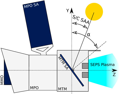
FIGURE 1. Sketch of BepiColombo in the YZ plane of the spacecraft reference frame and defined angles. The yellow disk represents the Sun, the dark gray squares two of the four T6 thrusters, while the dark blue areas are the solar cells-covered surfaces. The SEPS plasma expanding in space to generate thrust is indicated by the light blue region.

FIGURE 2

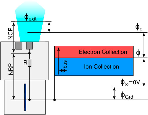
FIGURE 2. Relationships between the different potentials involved in the model. The red and blue regions depict the separation between electron and ion collecting areas of the MTM solar arrays. The NCP and NRP are the neutralizer coupling and reference potentials, respectively.

2.1 Mercury Transfer Module Solar Power Generator

The two 14m long MTM solar arrays, supporting over 40m² of solar cells, provide the power to operate the SEPS (≤11kW). They are located on the −X and +X sides of the spacecraft (see Figure 1) and are each made out of five panels. The solar cells are covered by radiation protecting dielectric coverglass and are connected in series through four small space-exposed conductive elements called interconnectors. They form strings of 40 cells oriented along the short edge of the SA, from a bus-bar connected to spacecraft ground to a bus-bar forming the high voltage terminal of the SA. All bus-bars run along the two long edges of the solar arrays, parallel to the X-axis of the spacecraft reference frame. Figure 3 shows a cropped section of a MTM solar panel, with the solar cells strings running vertically top to bottom from the grounded bus-bar to the high voltage bus-bar. The potential of the high voltage bus-bar is labeled ${\varphi }_{\text{bus}}$ and its absolute value is determined by ${\varphi }_{\text{bus}}=40\cdot dV+{\varphi }_{\text{Grd}}$, where dV is the voltage step occurring between two consecutive cells forming a string of 40. This voltage step is a function of the cell working temperature as it produces power, increasing with temperature. Therefore, as the distance to the Sun decreases, ${\varphi }_{\text{bus}}$ will increase from 57V to 105V above ${\varphi }_{\text{Grd}}$. A single panel counts around 5,535 interconnectors and 169 bus-bars. A single interconnector has an exposed surface area of $1.1\times 4.5{\text{mm}}^2$ and a bus-bar area of $77\times 4{\text{mm}}^2$ or $10\times 4{\text{mm}}^2$ depending on its location. The solar cell coverglass area is $80\times 44{\text{mm}}^2$.

FIGURE 3

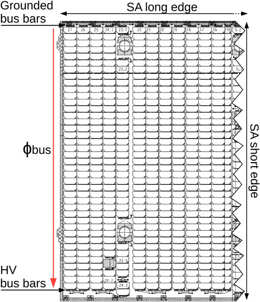
FIGURE 3. Cropped section of the photovoltaic assembly of a MTM solar panel showing main components.

While ideally the solar cells surface normal vector would keep SAA as close to $0^{\circ }$ as possible to maximize the power generation, increasing thermal loads on the solar panels while getting closer to the Sun requires progressively increasing this angle. Consequently, the solar arrays SAA will be varied within [4°, 73°]. Due to the mentioned spacecraft SAA allowed range, the solar cells will always present a nonnegligible cross-section to the T6 thrusters plasma backflow while the SEPS is operating. The MTM solar array rotation angle α is defined as the angle between the MTM solar cells normal vector and the +Y vector of the spacecraft reference frame (see Figure 1).

2.2 Solar Electric Propulsion System

The SEPS comprises four T6 gridded ion engines, two Power Processing Units (PPU), and the flow control units. The PPU controls and distributes the power generated by the solar arrays to the thrusters subsystems. To avoid arcing damage to galvanic insulation within the PPU, the voltage between the PPU housing, which is tied to spacecraft ground, and the PPU low voltage return is constrained to be less than 50V. To guarantee this requirement, a clamping network made out of back-to-back clamping diodes mounted in parallel to a bleeder resistor R connects the low voltage return to the spacecraft ground; see Figure 4. To protect the diodes, the whole SEPS is switched off if the voltage across R exceeds $\left|30\right|\text{V}$. This voltage is called the Neutralizer Reference Potential (NRP), as the SEPS low voltage return is the neutralizer reference point. Hence, for nominal operation of the SEPS, it is required that NRP$<\left|30\right|\text{V}$. The modeling results presented here were obtained with the goal of checking the amplitude of R prior to the mission to guarantee this requirement. The NRP is one of the key quantities to be monitored via the flight telemetries, as will be discussed later.

FIGURE 4

FIGURE 4. Electrical sketch of the SEPS. Current arrows represent electron flow and voltage arrows potential increase. The clamping network is composed of the bleeder resistor R and back-to-back diodes.

The T6 thruster was qualified for operation at 145mN, but its life-test was conducted at 125mN, the final nominal SEPS flight configuration (Randall et al., 2019). As the present model was made to verify the amplitude of R in the worst-case conditions, the simulations were run at 145mN. The T6 accelerates ionized xenon propellant from a discharge chamber through a potential gradient of 1850V between two grids and forms an ion beam of current $I_{\text{beam}}=2.167\text{A}$ at 145mN (Clark et al., 2019). Table 1 gives some key T6 working parameters at full thrust. $\dot{m}$ is the total xenon mass-flow (thruster plus neutralizer), ${\eta }_u$ is the propellant ionization efficiency, and ${\eta }_p$ the percentage of doubly charged ions. ${\varphi }_{\text{exit}}$ and $T_{\text{exit}}$ are the plume plasma parameters a few millimeters downstream of the thruster acceleration grid after charge neutralization.

TABLE 1

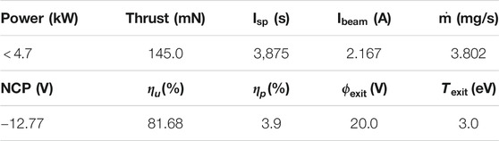
TABLE 1. T6 characteristics at full thrust in the BepiColombo flight qualification configuration. ${\varphi }_{\text{exit}}$ and $T_{\text{exit}}$ are derived from ground measurements (Snyder et al., 2012).

An electron current equal to $I_{\text{beam}}$ is delivered by a hollow cathode neutralizer (NTR) to guarantee currents balance and avoid charging. Such a device is composed of a hollow cylinder as the cathode and a keeper anode located downstream of the cathode exit. The cathode is made out of a low work function doped material, which releases thermionic electrons when heated above 1000°C (Goebel and Katz, 2008, pp. 19–136). To help trigger and sustain a stable plasma discharge inside the neutralizer, the PPU adjusts the keeper voltage ${\varphi }_{\text{k}}$ to maintain a predetermined constant current $I_k=4.21\text{A}$ flowing between the cathode and the keeper. This variation of ${\varphi }_{\text{k}}$ becomes especially necessary during flight since the keeper electrode would also collect current $I_{\text{p}}$ from the variable ambient plasma (Figure 4). ${\varphi }_{\text{k}}$ is then adjusted until $I_p=0\text{A}$. ${\varphi }_{\text{k}}$ is another quantity available from the flight telemetries from which quantitative insights might be obtained about the SEPS operation and its created plasma.

The neutralizer plasma expands downstream of the keeper in a quasineutral spot-like plasma. A potential gradient, called the Neutralizer Coupling Potential (NCP), will form between the ion beam (of local plasma potential ${\varphi }_{\text{exit}}$) and the neutralizer plasma (of local plasma potential ${\varphi }_{\text{NTR}}<{\varphi }_{\text{exit}}$) such that $\text{NCP}={\varphi }_{\text{NTR}}-{\varphi }_{\text{ref}}<0$ to ensure the neutralization of the SEPS created plasma (Goebel and Katz, 2008, pp. 19–136). This is illustrated in Figure 4. The NCP adjusts itself until $I_{\text{NTR}}=I_k+I_{\text{beam}}+I_{\text{LK}}$, where $I_{\text{NTR}}$ is the total electron current extracted from the neutralizer cathode. $I_{\text{LK}}$ is the net current collected by the spacecraft surfaces, from both environmental and SEPS backflow plasma, flowing back to the neutralizer via the bleeder resistor R; see Figure 4. Because of the mobility difference between ions and electrons, $I_{\text{LK}}$ will be predominantly electronic and will require a higher $I_{\text{NTR}}$ to be emitted by the neutralizer. A higher $I_{\text{NTR}}$ requires an increase of the cathode temperature, which in turn diminishes the neutralizer lifetime. This results in another constraint in the sizing of R: to ensure $I_{\text{LK}}<\left|50\right|\text{mA}$. The NCP is a linear function of $I_{\text{beam}}+I_{\text{LK}}$ ($I_k$ being kept constant) through the neutralizer current-potential characteristic. The ground measured characteristic of the T6 neutralizer is best fitted by $I_{\text{NTR}}=a\cdot \text{NCP}+b$ with $a=-0.56\text{A}/\text{V}$ and $b=-4.98\text{A}$. $I_{\text{LK}}$ was nonoccurring during ground testing of the SEPS and adds up in flight to $I_{\text{beam}}$ to induce a more negative NCP. Simulations output presented here allowed to confirm that setting $R=150\Omega$ was necessary to fulfill the requirements on the NRP and $I_{\text{LK}}$.

3 Electric Propulsion Induced Charging

An object immersed in plasma will acquire a floating potential ${\varphi }_f$ to balance the flux of electrons and ions to its surface (Lieberman and Lichtenberg, 2005, pp. 165–206). This potential is usually negative due to the higher electron mobility. In the case of BepiColombo, the plasma is predominantly a SEPS side product: the Charge-EXchange (CEX) backflow plasma, to which ambient environmental space plasma such as the solar wind adds up. CEX ions are created when electrons are transferred between fast thruster beam ions and slow neutral xenon atoms drifting away from the thruster, resulting in ions with ambient thermal velocities and fast neutrals. The CEX ions have low kinetic energies and are attracted toward the negatively charged spacecraft to reach most of its surfaces, joined by the electrons from the neutralizer and the ambient plasma (Markelov and Gengembre, 2006). From this plasma, each surface will collect currents and contribute to the S/C charging equilibrium depending on its electrical properties and connections to the rest of the spacecraft. Since the SEPS creates this dense plasma and forms a closed electrical loop through it between the neutralizer and the spacecraft, the SEPS plays a dominant role in the charging of BepiColombo. Both the SEPS and the MTM solar arrays influence the plasma charged species fluxes and make the BepiColombo frame potential ${\varphi }_{\text{Grd}}$ differ from ${\varphi }_f$, as described below.

Focusing on the SEPS role first, the neutralizer will maintain the required negative NCP between the SEPS low voltage return and the beam plasma potential ${\varphi }_{\text{exit}}$, driving ${\varphi }_{\text{Grd}}$ negative with respect to the local ${\varphi }_f$. The leakage current $I_{\text{LK}}$ through the clamping network bleeder resistor R from surfaces collected currents will induce the NRP, which will add to the NCP to make ${\varphi }_{\text{Grd}}$ even more negative. This is illustrated in the sketches of Figures 2, 4.

The solar arrays are the main contributor to $I_{\text{LK}}$, and by extension to the charging, as high electron currents get collected by the positively biased interconnectors and bus-bars (Ferguson and Hillard, 1995; Tajmar et al., 2009). SMART-1 telemetries showed that the plasma density varies within $\left[{10}^8,{10}^{15}\right]{\text{m}}^{-3}$ around the spacecraft, decreasing with increasing distance from the thrusters (Markelov and Gengembre, 2006; Tajmar et al., 2009). Assuming a bulk plasma temperature of 1eV and CEX densities $\in \left[{10}^{10},{10}^{12}\right]{\text{m}}^{-3}$ over the MTM SA, the sheath developed around the solar arrays will have a thickness ranging in $\sim \left[\mathrm{5,70}\right]\text{cm}$. Considering the millimetric scales of the interconnectors and bus-bars, those elements should only see the electron depleted region of the solar array sheath and have a minor contribution to the total collected current. However, experiments and flight data have shown that the interconnectors and bus-bars follow a Langmuir probe-like collection law, resulting in significant electron collection relative to their size when their biases get positive enough (Fujii and Abe, 2003). This behavior is attributed to secondary electrons released by the coverglass adjacent to the positively biased elements, produced by CEX and solar wind ion and electron impacts, as well as photoelectrons released from solar Lyman Alpha radiation (Lai, 2011, p. 53). These electrons are then attracted and collected by the interconnectors and bus-bars. This effect, coined “snapover,” occurs when portions of the interconnectors are biased well above the surrounding bulk plasma floating potential ${\varphi }_f$ (Hastings and Chang, 1989). With the two possible maximum absolute values of the NRP and the NCP ($30\text{V}$ and $12.77\text{V}$, respectively), and the maximum possible values of ${\varphi }_{\text{bus}}=105\text{V}$, a significant amount of interconnectors and bus-bars can be biased well above the local ${\varphi }_f$ and be subject to snapover, as illustrated in Figure 2. The electron currents collected by the solar arrays are thus expected to dominate the net spacecraft collected current balance.

The nature of the expected interactions between the thruster plasma and the spacecraft required the creation of a detailed geometric, physical, and electrical numerical model of BepiColombo, with sufficient spatial resolution over a simulation volume the scale of the spacecraft, with accurate reproduction of the plasma environment and electrical behaviors of the SEPS and the solar arrays. This is necessary for assisting mission design and improving incremental understanding of these phenomena.

4 Numerical Model

The open-source simulation package SPIS is a 3D electrostatic solver based on a Particle-In-Cell approach to compute the main moments of the plasma populations’ distribution functions and solves the Vlasov Poisson system in the unstructured mesh volume surrounding a meshed spacecraft. In addition, it computes the potential distribution on the meshed spacecraft surfaces from the balance of collected and emitted plasma currents together with conducted currents through the different surface materials to spacecraft ground which are electrical coupled (circuit solver part). This code is designed to simulate spacecraft charging in various environments (low-Earth orbits, geostationary, etc.) and, more recently, during EP operations (Thiebault et al., 2015). The present work uses SPIS v5.2.4 coupled with the AISEPS package (Wartelski et al., 2013). Due to the complexity and dimensions of the system, the present model of BepiColombo employs the Particle-In-Cell (PIC) formalism with a few significant departures from the pure approach in order to accommodate computational resource limitations. Code particularities and details are hereby presented.

4.1 Plasma Populations

Due to the high plasma densities involved and the large computation volume, it is computationally too expensive to simulate every physical particle on a standard workstation. The PIC approach is employed instead to reduce the total number of particles by using macroparticles. Each macroparticle represents a great number of physical particles.

BepiColombo ion beam macroparticles, ${\text{Xe}}_{\text{fast}}^{+}$, ${\text{Xe}}_{\text{fast}}^{++}$, and nonionized xenon, Xe_slow, are injected in the simulation volume at the thruster exit surface. The parameters of Table 1 are used to set the respective mass-flow rates of neutral, singly, and doubly ionized xenon propellant according to a model derived from ground measured thruster plumes (Tajmar et al., 2000). The ions density distribution over the thruster grid varies according to a radial Gaussian distribution with a standard deviation fitted to the ground measured T6 beam divergence of 13.54° at 145mN. The ions velocity distribution is adjusted to reproduce the T6 concave ion optics (Snyder et al., 2012). The neutrals macroparticles are injected following a radial cosine distribution, while their velocity distribution is a randomized cosine probability distribution. Accurately reproducing the density of these populations and velocity distributions is important in order to obtain a sound CEX density distribution in the surrounding of the thruster plume. Details necessary for the numerical T6 definition are given in the Supplementary Material.

The CEX ions macroparticles are created in the simulation volume through a Monte Carlo collision algorithm. A fast ion is changed into a slow charge-exchange ion at random neutral thermal velocity according to a collision probability function taking empirically determined cross-sections as argument (Miller et al., 2002). The two CEX collisions implemented in this model are as follows:

$\{\begin{array}{c}{\text{Xe}}_{\text{fast}}^{+}+{\text{Xe}}_{\text{slow}}\to {\text{Xe}}_{\text{fast}}+{\text{Xe}}_{\text{slow}}^{+}\\ {\text{Xe}}_{\text{fast}}^{++}+{\text{Xe}}_{\text{slow}}\to {\text{Xe}}_{\text{fast}}+{\text{Xe}}_{\text{slow}}^{++}\end{array}.$

Since the resulting ${\text{Xe}}_{\text{fast}}$ population does not contribute to the charging, they are not generated in order to keep the number of macroparticles down. CEX collisions have larger cross-sections than other ion-neutral and recombination collisions (Tajmar et al., 2009). With the respective properties of the T6 ions and neutrals, the ${\text{CEX}}^{+}$ reaction has a cross-section of $\sim 4.28\cdot {10}^{-19}\text{m}$ and the ${\text{CEX}}^{++}$ of $\sim 1.67\cdot {10}^{-19}\text{m}$. Comparatively, the singly charged ion with neutral elastic (scattering) collision has a cross-section of $\sim 1.23\cdot {10}^{-20}\text{m}$, while the doubly charged ion with neutral elastic has a cross-section of $\sim 1.74\cdot {10}^{-20}\text{m}$. Therefore, CEX collisions play the predominant role in the creation of the diffuse plasma backflow and its interactions with the spacecraft. Other interactions such as ion-neutral elastic collisions were not available in SPIS at the time of the study but will be implemented in the next phase.

In the classic PIC kinetic formalism, the tetrahedra composing the 3D mesh of the simulation domain need to be smaller than the local Debye length in order to resolve the sheaths and the electron dynamics. With submillimetric Debye lengths downstream of the thruster, respecting this condition in a simulation volume encapsulating BepiColombo would require an amount of memory exceeding available workstation capabilities. An alternative is to treat the neutralizer electrons as an isothermal fluid population whose density over the simulation mesh is determined by the local plasma potential according to Boltzmann’s relation:

$n_e=n_{\text{ref}}{e}^{\frac{e\left({\varphi }_p-{\varphi }_{ref}\right)}{T_e}},(1)$

where e is the elementary charge, $n_e$, ${\varphi }_p$, and $T_e$ are the electron density, plasma potential, and electron temperature, respectively, evaluated on the simulation grid points. $T_e$ is expressed in energy units. $n_{\text{ref}}$ is the electron density at grid points, where ${\varphi }_p={\varphi }_{\text{ref}}$ and $T_e=T_{\text{ref}}$ simultaneously, which are predetermined fixed values. In the present case, ${\varphi }_{\text{ref}}={\varphi }_{\text{exit}}$ and $T_{\text{ref}}=T_{\text{exit}}$ are the T6 thruster exit conditions reported in Table 1. However, ground and flight measurements, as well as numerical simulations, have shown that the electron population temperature of a freely expanding thruster plasma plume is better described by a polytropic law (Tajmar et al., 2009; Dannenmayer and Mazouffre, 2013). Due to code limitations at the time of the present study, and in order to allow a simplified yet physically meaningful representation of the coupling between the T6 thruster plume and BepiColombo, the quasineutrality assumption in the simulation domain (where $n_e=n_i$) was necessary in order to obtain a nonisothermal fluid electron population with the polytropic law:

$T_e{n}_e^{1-\gamma }=C,(2)$

where C is a constant and γ is the polytropic index, with $\gamma =1$ corresponding to the isothermal case and $\gamma =5/3$ to an adiabatic plasma. As major drawbacks, the forced quasineutrality assumption prevents the sheath from being correctly described in the vicinity of the spacecraft surfaces, especially the S/A coverglass, which is impacted by CEX ions. In addition, the taken polytropic assumption does not capture the electron polytropic index variations in collisionless plasma plume expansion (Hu and Wang, 2017; Merino et al., 2020). Given these constraints, a sensitivity analysis was performed using an adjustable gamma value in order to explore its influence on the plume-spacecraft coupling parameter space (not reported in the present article).

4.2 Potential Solver

To obtain the plasma potential in the simulation volume, the usual PIC approach is to solve Poisson’s equation:

${\nabla }^2{\varphi }_p=-\frac{e}{{\epsilon }_0}\left(n_i-n_e\right),(3)$

where ${\epsilon }_0$ is the vacuum permittivity and $n_i$, $n_e$ are the densities of the simulated ions and electrons on the grid. For clarity, this equation and the following ones are given for a singly charged ion population. In practice, $n_i$ is replaced with ${\displaystyle {\sum }_k{Z}_k{n}_{i_k}}$, the sum over the ion subpopulations with their respective charge number $Z_k$. In SPIS-AISEPS, Poisson’s equation can only be solved in the full kinetic formalism or using a fluid isothermal electron population. Obtaining consistent spacecraft-plasma interactions requires a plasma volume around the spacecraft with realistic properties, e.g., with variable electron temperature $T_e$. Together with computational power limitations that forbid using the full kinetic approach, this called for an alternative to Poisson’s equation. The only available solution in AISEPS was to estimate the plasma potential distribution in the volume by combining Eq. 2 and the Vlasov equation together with the quasineutrality hypothesis to obtain the following:

${\varphi }_p=\frac{\gamma T_{\text{ref}}}{e\left(\gamma -1\right)}\left[{\left(\frac{n_i}{n_{\text{ref}}}\right)}^{\gamma -1}-1\right]+{\varphi }_{\text{ref}}.(4)$

This method gives the local plasma potential as an explicit law of the local ion density everywhere in the domain. In the isothermal case, the equivalent approach is to invert Boltzmann’s relation Eq. 1 with the quasineutral assumption to determine ${\varphi }_p$, as an alternative to solving Poisson’s equation. In SPIS, ${\varphi }_{\infty }$ is set to $0\text{V}$ by default and this value has no effect on the computed electric potentials of both the plasma and the simulated surfaces, contrary to ${\varphi }_{\text{ref}}$. The value given to ${\varphi }_{\infty }$ is only shown for completeness as it is a relevant user parameter. Moreover, in general ${\lim }_{n_e\to 0}{\varphi }_p\ne {\varphi }_{\infty }$, even if it will be the goal to obtain ${\lim }_{n_e\to 0}{\varphi }_p=0\text{V}$ by appropriately setting γ, $T_{\text{ref}}$, and ${\varphi }_{\text{ref}}$.

The electron temperature variation is obtained by replacing the constant in Eq. 2 with the thruster reference values:

$T_e=T_{\text{ref}}{\left(\frac{n_i}{n_{\text{ref}}}\right)}^{\gamma -1}.(5)$

Measurements in space and laboratories report $\gamma \in \left[1;1.3\right]$, thus lower than the adiabatic coefficient $5/3$, within some cases the polytropic index spatially varying in the plume of plasma thrusters (Nakles et al., 2007; Dannenmayer and Mazouffre, 2013). In the current work, γ will be varied between the isothermal case ($\gamma =1$) and the adiabatic one ($\gamma =5/3$).

Figure 5 displays ${\varphi }_p$ and $T_e$ as a function of the expected range of ${\text{n}}_{\text{e}}$, calculated using Eqs. 1, 4, 5 for $\gamma \in [1,5/3]$, ${\varphi }_{\text{ref}}=20\text{V}$, and $T_{\text{ref}}=3\text{eV}$. The $\gamma =1$ curve shows that the plasma potential goes to $-\infty$ as the plasma density decreases, showing the limitation of the isothermal condition with the quasineutrality assumption. For $\gamma \ne 1$, ${\varphi }_p$ goes to horizontal asymptotes at low densities and always stays positive for $\gamma \ge 1.18$. The value $\gamma =1.18$ is obtained by solving Eq. 4 for γ giving ${\varphi }_p=0\text{V}$, when $n_i=0{\text{m}}^{-3}$, ${\varphi }_{\text{ref}}=20\text{V}$, and $T_{\text{ref}}=3\text{eV}$. Using the polytropic model for the electron cooling and the quasineutrality allows controlling the plasma potential in the simulation volume. This is an unorthodox PIC approach compared to solving Poisson’s equation in the sense that the volume potentials are ad hoc: set a chosen value of γ in order to obtain potential gradients, which result in expected CEX backflow density distributions and fluxes to the spacecraft surfaces. A similar approach has been successfully used to reproduce SMART-1 observed SEPS-induced charging (Tajmar et al., 2009). The present model will be calibrated with BepiColombo flight telemetries in the next stage of the study.

FIGURE 5

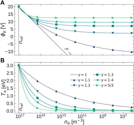
FIGURE 5. (A) Plasma potential ${\varphi }_p$ and (B) electron temperature $T_e$ as a function of the plasma density $n_e$ for different γ and with ${\varphi }_{\text{ref}}={\varphi }_{\text{exit}}=20\text{V}$, $T_{\text{ref}}=T_{\text{exit}}=3\text{eV}$.

4.3 Circuit Solver

To reproduce the spacecraft-plasma coupling through current collection and emission, the numerical model needs to include the electrical properties of the surface materials. As a trade-off between detailed surfaces and numerical mesh density, each spacecraft surface is represented by its external surface coating material and is included in the model as a macroscopic electrical node. SPIS allows the definition of the material electric and physical properties such as surface and bulk conductivity, electron and protons induced secondary electron emission, and photoemission yields (for the main ones). Each surface node is linked to the spacecraft ground through an equivalent RC electrical circuit. Differential charging occurring between dielectric surfaces and the S/C ground is computed, accounting for dielectric thicknesses and surface and volume conductivity. Sources representing thrusters and neutralizers can also be linked to the circuit solver. A source can either be a physical source for which an actual PIC population emission in the volume draws a corresponding current from the circuit or a virtual source that only draws a current but does not generate macroparticles.

Since the quasineutrality assumption precludes reproducing the sheaths, the electron flux to the spacecraft surfaces is calculated using the following electron collection model:

$\{\begin{array}{cc}{J}_e=J_{e_0}\exp \left(\frac{e\left({\varphi }_s-{\varphi }_p\right)}{T_e}\right),& \text{if}{\varphi }_s-{\varphi }_p<0,\\ J_e=J_{e_0}\left(1+\frac{e\left({\varphi }_s-{\varphi }_p\right)}{T_e}\right),& \text{if}{\varphi }_s-{\varphi }_p>0,\end{array}(6)$

where $J_{e_0}=-e{n}_e\sqrt{e{T}_e/2\pi m_e}$ is the thermal current density in the bulk plasma and ${\varphi }_s$ the potential of the collecting surface. In the quasineutral approach, $J_{e_0}$ is computed directly at the surface nodes, since there is no sheath. The case ${\varphi }_s-{\varphi }_p<0$ uses the typical formula encountered for the Debye sheath retarded electron current, when the surface is biased negatively with respect to the bulk plasma (Lieberman and Lichtenberg, 2005, pp. 165–206). The case ${\varphi }_s-{\varphi }_p>0$ models the surface collection area (sheath) increase when the surface is biased more positively than the local plasma and is referred to as the Orbital Motion Limited (OML) law (Lieberman and Lichtenberg, 2005, pp. 165–206). Because sheaths can not be reproduced using the quasinetural assumption, this collection area increase is numerically accounted for by the OML law. Using this law is consistent as long as the Debye sheaths thickness is large compared to the size of the spacecraft surface features. It however remains a simplistic approach considering the geometrical complexity of some of the surfaces. Ion currents are calculated by counting how many ion macroparticles hit a given surface. This is then translated into current by taking into account the ion macroparticle weight (how many physical particles this macroparticle represents) and charge number.

4.4 Numerical Spacecraft Systems

BepiColombo surfaces are made from a variety of materials to meet the mission thermal requirements and to mitigate differential charging. The present model includes 20 different materials, corresponding to 20 different nodes in the circuit solver. In Figure 6, each color represents a different node/material.

FIGURE 6

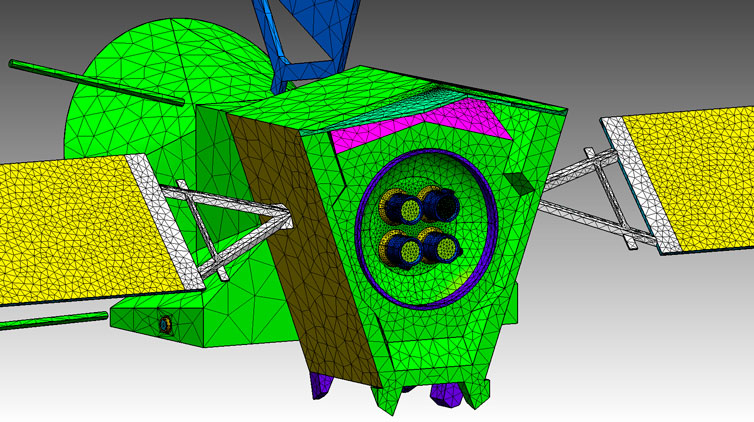
FIGURE 6. Section of BepiColombo geometrical model, showing the thruster bay with the local mesh refinements. Each color corresponds to a different material and electrical node.

Simulating the real coupling between the neutralizer plasma and the ion beam is beyond the capabilities of the present model due to the use of the quasineutral solver. To reproduce the impact of the NCP on spacecraft charging, the alternative was to define an equivalent virtual SEPS in the electrical circuit. This virtual source reproduces the total net current draw of the entire SEPS (see the corresponding dashed rectangle in Figure 4), i.e., $I_{\text{beam}}+I_{\text{NTR}}+I_{\text{LK}}$ from the spacecraft equivalent circuit, as a single electrical node. This node does not emit macroparticles nor modify the electron population distribution. $I_{\text{beam}}$ corresponding to the desired thrust level is calculated by the virtual source using the same input file as the macroparticles source. The fit to the ground measured current-potential characteristic of the neutralizer ($I_{\text{NTR}}=a\cdot \text{NCP}+b$) is then used by the virtual SEPS to set the potential of the node (the NCP) to a value verifying $I_{\text{NTR}}=I_{\text{beam}}+I_{\text{LK}}$. For example, if $I_{\text{LK}}=0\text{A}$, then the NCP takes the value reported in Table 1 for a thrust of $145\text{mN}$. The NCP thus varies with both the desired thrust level and the $I_{\text{LK}}$ collected from the plasma. When nominal neutralization is simulated, only $I_{\text{LK}}$ is drawn from the rest of the circuit. The virtual SEPS is connected to the spacecraft ground via the bleeder resistor R in the circuit solver and the difference between the NCP and ${\varphi }_{\text{Grd}}$ gives the NRP developed across R (see Figure 4).

Due to the interconnectors and bus-bars small dimensions and large number, their reproducing in the spacecraft geometrical model is not possible. Likewise, simulating their complex interactions with the CEX plasma, solar wind, and radiation is beyond the capabilities of SPIS. Instead, the AISEPS package implemented a simplistic approach to the interconnector plasma collection processes based on the following strong assumption: owing to the interconnectors small size, their potentials are shielded by the surrounding coverglasses and are not perceived by the bulk plasma flowing toward the solar cells. Only once inside the coverglass sheath can the plasma feel the interconnector potentials. As a result, the solar cells side of the solar array is simplified as a being entirely made out of coverglass, visible in yellow in Figure 6. Being a dielectric, the coverglass develops local differential surface potentials during plasma collection. The interconnectors potential distribution from ${\varphi }_{\text{Grd}}$ to ${\varphi }_{\text{bus}}$ is analytically discretized unto the solar array at the circuit solver level but is not developed on the surface mesh and in the simulation volume. Each node of the solar array active side therefore possesses its own coverglass potential visible to the surrounding plasma and its own interconnector potential stored with the circuit solver and used for the current collection computation. Like the rest of the S/C surfaces, the plasma flux to the solar cells is calculated with the electron collection model (Eq. 6) and by counting impacting ion macroparticles, only taking into account the coverglass surface potentials. A user-defined function is then used to reproduce the theoretical or empirical interconnector current-potential characteristic. At each node, the incoming plasma species, charge, and energy, as well as local surface potentials (coverglass and interconnector) and local plasma potential, are evaluated by this function. It then discriminates whether the ions and electrons reaching the node are collected by the corresponding local coverglass or interconnector. This function can be viewed as a probability function for the node interconnector to either collect an electron or an ion. In the results presented here, the used function is the one that was found to reproduce the SMART-1 solar arrays observed collected currents (Wartelski et al., 2013).

5 Results

The outputs of the simulations are presented here to highlight the effects of the model specificity and their impact on the charging of BepiColombo. The potential for improving key aspects of the numerical modeling of electric propulsion-spacecraft charging through calibration with flight telemetries and future code improvements are discussed. This is the first step toward a more comprehensive in-flight characterization and description of the behavior of electrical thruster plumes in space. Presented results are from simulations ran at 145mN and with $\alpha ={90}^{\circ }$, unless otherwise specified (see Figure 1).

5.1 Solar Electric Propulsion System Plasma Generation

The thruster ions (${\text{Xe}}^{+}$$+$${\text{Xe}}^{++}$) and neutral density distributions obtained from the calibrated T6 model are shown in Figure 7, for the conditions of Table 1. The shape of the ion beam due to the T6 concave ion optics is reproduced and results in a focal point $18\text{cm}$ downstream of the grids; see Figure 7A. The thruster parameters were adjusted for the focal point location to match the values measured during ground testing. As a hollow cathode neutralizer typically has a low ionization efficiency, neutrals were also injected at the position of the neutralizer exit to more accurately reproduce the neutral xenon distribution in volume, which is critical for the CEX cloud creation. The neutral density maximum above the neutralizer is visible in Figure 7B and an asymmetry in the CEX density distribution at the neutralizer position was indeed observed in the simulation outputs (not reported here).Whereas the SEPS primary ions are negligibly affected by the plasma potential gradients in the simulation volume, the CEX ions follow the potential gradient-generated electric fields to eventually enclose the entire spacecraft. CEX ions are indeed generated within the thruster beam where the plasma potential (${\varphi }_{\text{exit}}=20\text{V}$) is more positive than the plasma potentials in the volume (see Figure 5A) and the negatively charged spacecraft. Carefully establishing the SEPS generated plasma potential via the potential solver is therefore essential to obtain consistent plasma dynamics and spacecraft charging levels. To validate the use of the quasineutral solver, Figure 8 compares the SEPS plasma potential distribution downstream of the T6 in the isothermal case $\gamma =1$, resolved with the quasineutral solver Eq. 4 and with Poisson’s Eq. 3 for the ground measured ${\varphi }_{\text{ref}}=20\text{V}$ and $T_{\text{ref}}=3\text{eV}$. Figures 8A,B show that the plasma potentials in the thruster plume and CEX cloud are similar with both potential solvers. As highlighted in Figure 5A, the isothermal assumption produces nonphysical negative plasma potentials only a few centimeters away from the beam centerline as the density decreases, regardless of the potential solver type. This would result in unrealistic levels of spacecraft charging, as in both cases, the OML model uses the bulk plasma properties to compute the surfaces collected currents. Employing a polytropic index greater than one is therefore necessary to reproduce the observed in-flight spacecraft charging levels. For $\gamma >1$, Boltzmann’s relation does not hold anymore and, with the version of SPIS available at the time of the study, only the quasineutral solver was capable of handling a nonisothermal fluid electron population.

FIGURE 7

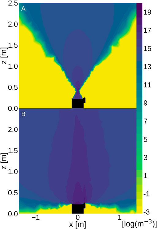
FIGURE 7. Density mappings at full thrust of (A) the total ion beam $\left({\text{Xe}}^{+}+{\text{Xe}}^{++}\right)$ and (B) the neutrals flowing out of the thruster grids and neutralizer contiguously attached to the right of each thruster at $x\simeq 0.18\text{m}$.

FIGURE 8

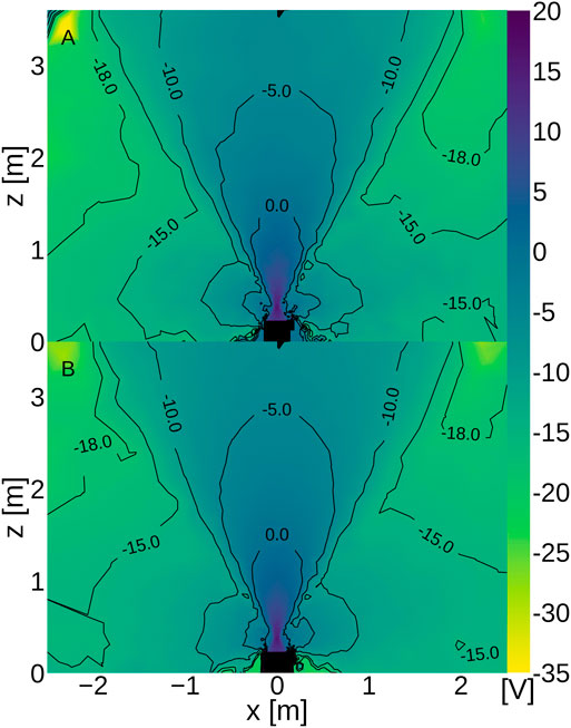
FIGURE 8. Plasma potential mapping downstream of the T6 thruster in the isothermal case calculated with (A) the quasineutral solver and (B) the Poisson solver, with ${\varphi }_{\text{ref}}=20\text{V}$, $T_{\text{ref}}=3\text{eV}$.

Figures 9, 10 display the entire simulation volume for the distribution of the total plasma density (ion beam + CEX) and plasma potential, respectively, for $\gamma =1.18$, ${\varphi }_{\text{ref}}=20\text{V}$, and $T_{\text{ref}}=3\text{eV}$, obtained with the quasineutral solver. With $\alpha ={90}^{\circ }$, the solar arrays are parallel to the XY plane and extend from $x=\left|2.9\right|\text{m}$ to $x=\left|15.2\right|\text{m}$. For these two figures, all spacecraft surface potentials were fixed to $0\text{V}$ to remove their negative floating potentials to improve the visibility of the colormap scaling in Figure 10. Figure 10 shows that, for $\gamma =1.18$, the plasma potential is positive everywhere, even in the lowest density regions such as the back of the MTM solar arrays, in accordance with Eq. 4. This is in contrast with the isothermal case of Figure 8. Adequate CEX ions dynamics and subsequent surface charging are therefore possible.

FIGURE 9

FIGURE 9. Mapping of the plasma density around BepiColombo in the XZ plane for an arbitrary fixed spacecraft ground ${\varphi }_{\text{Grd}}=0\text{V}$ and $\gamma =1.18$.

FIGURE 10

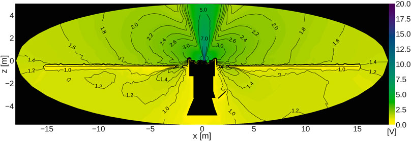
FIGURE 10. XZ mapping of the plasma potential around BepiColombo, for the same conditions as Figure 9. The plasma potential stays positive everywhere in the volume, as expected.

Taking the plasma densities right over the MTM solar arrays from Figure 9 and the corresponding electron temperatures (no reported here), the Debye sheath thicknesses at these locations range inside $\sim \left[7;20\right]\text{cm}$, increasing as one moves away from the thruster position. The typical size of a solar cell is therefore either equivalent or smaller than the local Debye sheath thickness. The OML law portion of the electron collection model, which applies if the collecting surface potential is more positive than the surrounding plasma (Eq. 6), requires the Debye sheath thickness to be much larger than the scale of the collecting area (Lieberman and Lichtenberg, 2005, pp. 165–206). For the simulation conditions reported here, the portion of the MTM coverglass where the Debye sheath thickness is of the order of the solar cell size is unfortunately also the only portion where the coverglass is biased more positively than the surrounding plasma. At these locations, the OML law is misused and would result in a local overcollection of electrons. The majority of the MTM coverglass area however respects the conditions of the electron collection model. The other S/C surfaces were all observed to be negatively biased with respect to the surrounding plasma, so even if their dimensions were bigger than the local Debye sheath, the electron collection model stayed valid. Overall, this supports the use of the electron collection model implemented in SPIS-AISEPS as a reasonable approach to estimate the electron currents on the most significant spacecraft surfaces, despite not being able to resolve the Debye sheaths.

In Figure 9, the CEX could reach every corner of the simulation volume as expected. The characteristic CEX side lobes are clearly visible, and it is interesting to notice how the CEX ions develop backward lobes through the yokes of the MTM solar arrays, for $x\in \left[-5,-2\right]\text{m}$ and $x\in \left[\mathrm{2,5}\right]\text{m}$ in Figure 9. The minimum plasma densities in the volume are of the order of ${10}^8{\text{m}}^{-3}$, which is one and two orders of magnitude greater than the solar wind density at $0.3\text{AU}$ and $1\text{AU}$, respectively (Barouch, 1977). In consequence, the solar wind contribution to the spacecraft charging is to the second order compared to the CEX plasma and is not included in the present model. The comparison between the CEX density distribution in Figure 9 and the primary ion beam density distribution displayed in Figure 7A shows that the primary ions play no direct role in the spacecraft charging since they can never intersect a S/C surface and have a kinetic energy too great to be deflected by the developed potential gradients. An animation of the transient expansion of the plasma can be found in the Supplementary Material. It shows the total plasma density in a logarithmic scale, from the initial state of a simulation (thruster off) to near equilibrium, for the conditions of Figure 9 but with $\alpha ={60}^{\circ }$ to better display the solar arrays.

5.2 Influence of Model Parameters

The simplifications and uncertainties of the BepiColombo model have various impacts on spacecraft charging. The extend of these impacts will be covered in the following study in which the in-flight SEPS telemetries will serve as calibration data for the numerical model, allowing new refinements and consequently increasing the reliability and confidence in preflight simulation of SEPS-induced charging. To illustrate the interest of such a process, the impact of the value of γ on the equilibrium electrostatic charging of BepiColombo is reported in Figure 11. In this figure and Figure 12, each data point is an average on the ten last simulation time-steps once equilibrium was reached. The plain lines connecting data points serve as a visualization guide. The standard deviation from the mean is shown as red vertical error bars. In most cases, the error bars are smaller than the marker size. In Figure 11, BepiColombo’s frame potential ${\text{Φ}}_{\text{Grd}}$, the NRP, the interconnector collected current $I_{\text{IC}}$, and the leakage current through the bleeder resistor $I_{\text{LK}}$ are reported for $\gamma \in \left\{1.0,1.1,1.2,1.3,1.4,5/3\right\}$. This is motivated by the fact that the polytropic index has been reported to spatially vary in the plume of a plasma thruster (Nakles et al., 2007); therefore, choosing an arbitrary value of γ is an approximation to the real cooling behavior. The NRP, and by extension $I_{\text{LK}}$, will be the only of these four quantities to be directly available from the SEPS telemetries. Confirming the observations of Figure 8, $\gamma =1$ produces the worst-case charging as the leakage current exceeds the $50\text{mA}$ design requirement while the NRP is close to the $30\text{V}$ limit. The NRP might wander above $30\text{V}$ and the SEPS would not be able to operate nominally. For all values of γ, it is clear that the current collected by the interconnectors and bus-bars of the MTM solar arrays dominates the total current at equilibrium, as $I_{\text{LK}}$ and $I_{\text{IC}}$ magnitudes are close and follow the same trend. The fact that $\gamma =1$ produces the worst-case situation is explained by two factors: 1) BepiColombo is immersed into a plasma whose potential is negative everywhere (see Figure 8A) and 2) as ${\varphi }_{\text{exit}}$ is used as a fixed parameter here, the SEPS NCP keeps the spacecraft ground more positive than the surrounding floating potential, meaning that a higher number of the MTM interconnectors are biased more positively than ${\text{Φ}}_f$ compared to simulations with $\gamma >1$ (see Figure 2). At higher values of γ, the plasma potential in the volume gets more and more positive and the magnitude of $I_{\text{IC}}$ decreases as a smaller proportion of interconnectors are biased above the plasma floating potential. The case $\gamma =1.18$ is indicated by the vertical dotted line in Figure 11.

FIGURE 11

FIGURE 11. Influence of γ on four simulation outputs of interest, for the input parameters of Table 1 and $\alpha ={90}^{\circ }$.

FIGURE 12

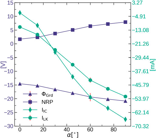
FIGURE 12. Influence of the MTM solar arrays angle α on the four simulation outputs, for $\gamma =1.18$, and the standard input parameters of Table 1.

SMART-1 flight telemetries showed a cyclic variation of the spacecraft ground potential coinciding with the spacecraft orbital period. Numerical modeling allowed to attribute these variations to the rotation of the spacecraft solar arrays as in order to keep a constant SAA along the orbit, their α was varying accordingly (Tajmar et al., 2009). This change in α meant that the solar arrays interconnectors were exposed to regions of the CEX backflow plasma of varying density and temperature. Figure 12 shows that for fixed simulation inputs, a similar dependency between the interconnectors collected current (and therefore with ${\text{Φ}}_{\text{Grd}}$ and the NRP) and α is expected for BepiColombo. At $\alpha ={90}^{\circ }$, the MTM solar arrays are face-on to the SEPS backflow and at a given radial distance away from the thruster exit, all interconnectors are exposed to a plasma of approximately the same density and temperature. At $\alpha =0^{\circ }$, the solar arrays are edges-on to the backflow and portions of the interconnectors are immersed in plasma of lower density and temperature, resulting in a lower $I_{\text{IC}}$.

6 Conclusion

BepiColombo’s seven years trip to Mercury presents a unique opportunity to improve current modeling and understanding of spacecraft charging induced by the operation of a SEPS thanks to soon-to-be available flight telemetries.

Upon creating a numerical representation of the T6 thruster plasma plume reproducing ground measured plume properties, the charge-exchange collisions generate a low-energy backflow plasma, which contacts all space-exposed surfaces by following plasma potential gradients down to the negatively charged spacecraft. Due to the electrostatic nature of this diffusion, establishing physically sound plasma potentials in the simulation volume is key to obtaining a self-consistent spacecraft charging process. While the erroneous isothermal assumption leads to nonphysical and unusable results, a polytropic process with $\gamma >1$ delivers acceptable plasma potentials and spacecraft charging levels while also being a simplistic approach with physical and numerical limitations. The major drawback is the ad hoc nature of the plasma potential generation by choosing an appropriate value of γ and the impossibility of reproducing sheaths around the spacecraft, requiring a simplified electron collection model for computing plasma collected currents. Future work will instead employ a new potential solver capable of solving Poisson’s equation together with a polytropic electron population in order to resolve sheath dynamics. Key to the charging, the large currents collected by numerous tiny biased interconnectors located on the solar arrays are also implemented through an oversimplistic approach in the current model. Despite these limitations, the current model is capable of reaching a dynamic equilibrium between the currents emitted by the SEPS and the ones collected by the spacecraft surfaces, giving expected values of spacecraft potential charging.

The strong influence of some of the model numerical and physical parameters on the simulations’ outputs, such as the NRP, demonstrates how the flight telemetries of BepiColombo will allow validating and improving the new electron cooling algorithms, plasma potential solver, and interconnectors model included in the latest version of SPIS. This will in turn help improve preflight assessments of EP-induced charging and will provide invaluable insight into the variability of SEPS operation in space compared to on-ground.

Data Availability Statement

The raw data supporting the conclusions of this article will be made available by the authors without undue reservation.

Author Contributions

This work has been conducted by FF as part of an ESA Young Graduate Traineeship initiated and supervised by OS. FC brought expertise on numerical simulation aspect (SPIS) and CC on plasma physics and electric propulsion.

Conflict of Interest

The authors declare that the research was conducted in the absence of any commercial or financial relationships that could be construed as a potential conflict of interest.

Supplementary Material

The Supplementary Material for this article can be found online at: https://www.frontiersin.org/articles/10.3389/frspt.2021.639819/full#supplementary-material.

Nomenclature

SEPS Solar electric propulsion system

SPIS Spacecraft plasma interaction system

MTM Mercury transfer module

SA Solar array

SAA Solar aspect angle

NRP Neutralizer reference potential

NCP Neutralizer coupling potential

CEX Charge-exchange

I_beam Ion beam current

I_IC Current collected by the interconnectors

I_LK Leakage current through the bleeder resistor;

α MTM solar array rotation angle

γ Polytropic index

${\varphi }_{\mathbf{Grd}}$ Spacecraft ground potential

${\varphi }_{\text{exit}}$, ${\mathit{T}}_{\mathbf{exit}}$ Plasma potential and electron temperature at the thruster exit

${\varphi }_{\text{ref}}$, ${\mathit{T}}_{\text{ref}}$ Quasineutrality solver reference plasma potential and electron temperature

${\varphi }_{\text{bus}}$ MTM solar array high voltage bus-bar potential

${\varphi }_{\infty }$ Undisturbed space plasma potential.

References

Barouch, E. (1977). Properties of the solar wind at 0.3AU inferred from measurements at 1AU. J. Geophys. Res. 82, 1493–1502. doi:10.1029/JA082i010p01493

CrossRef Full Text | Google Scholar

Benkhoff, J., Van Casteren, J., Hayakawa, H., Fujimoto, M., Laakso, H., Novara, M., et al. (2010). BepiColombo-Comprehensive exploration of Mercury: mission overview and science goals. Planet. Space Sci. 58, 2–20. doi:10.1016/j.pss.2009.09.020

CrossRef Full Text | Google Scholar

Clark, S., Randall, P., Lewis, R., Marangone, D., Goebel, D., Chaplin, V., et al. (2019). “BepiColombo–solar electric propulsion system test and qualification approach”. in Proceedings of the 36th International Electric Propulsion Conference, Vienna, Austria, 15–20 September, 2019, 1–20.

Google Scholar

Dannenmayer, K., and Mazouffre, S. (2013). Electron flow properties in the far-field plume of a Hall thruster. Plasma Sourc. Sci. Technol. 22, 035004. doi:10.1088/0963-0252/22/3/035004

CrossRef Full Text | Google Scholar

Ferguson, D., and Hillard, G. (1995). Space measurement of electron current collection by space station solar arrays. AIAA Paper 1995-0486. doi:10.2514/6.1995-486

CrossRef Full Text | Google Scholar

Fujii, H., and Abe, T. (2003). Current collection and discharges on high voltage solar array for space use in plasma. IEEE Trans. Plasma Sci. 31, 1001–1005. doi:10.1109/TPS.2003.818448

CrossRef Full Text | Google Scholar

Goebel, D. M., and Katz, I. (2008). Fundamentals of electric propulsion: ion and Hall thrusters. New York, NY: John Wiley & Sons, 19–136. doi:10.1002/9780470436448

CrossRef Full Text

Gollor, M. (2011). Accommodation aspects of electric propulsion with power processing units and the spacecraft. AIAA Paper 2011-5651. doi:10.2514/6.2011-5651

CrossRef Full Text | Google Scholar

Hastings, D. E., and Chang, P. (1989). The physics of positively biased conductors surrounded by dielectrics in contact with a plasma. Phys. Fluids B: Plasma Phys. 1, 1123–1132. doi:10.1063/1.858982

CrossRef Full Text | Google Scholar

Hu, Y., and Wang, J. (2017). Fully kinetic simulations of collisionless, mesothermal plasma emission: macroscopic plume structure and microscopic electron characteristics. Phys. Plasmas. 24, 033510. doi:10.1063/1.4978484

CrossRef Full Text | Google Scholar

Lai, S. T. (2011). Fundamentals of spacecraft charging: spacecraft interactions with space plasmas. Princeton, NJ: Princeton University Press, 53. doi:10.2307/j.ctvcm4j2n

CrossRef Full Text

Lieberman, M. A., and Lichtenberg, A. J. (2005). Principles of plasma discharges and materials processing. New York, NY: John Wiley & Sons, 165–206. doi:10.1002/0471724254

CrossRef Full Text

Markelov, G., and Gengembre, E. (2006). Modeling of plasma flow around SMART-1 spacecraft. IEEE Trans. Plasma Sci. 34, 2166–2175. doi:10.1109/TPS.2006.879098

CrossRef Full Text | Google Scholar

Merino, M., Fajardo, P., Giono, G., Ivchenko, N., Gudmundsson, J.-T., Mazouffre, S., et al. (2020). Collisionless electron cooling in a plasma thruster plume: experimental validation of a kinetic model. Plasma Sourc. Sci. Technol. 29, 035029. doi:10.1088/1361-6595/ab7088

CrossRef Full Text | Google Scholar

Miller, J. S., Pullins, S. H., Levandier, D. J., Chiu, Y.-h., and Dressler, R. A. (2002). Xenon charge exchange cross sections for electrostatic thruster models. J. Appl. Phys. 91, 984–991. doi:10.1063/1.1426246

CrossRef Full Text | Google Scholar

Nakles, M. R., Brieda, L., Reed, G. D., Hargus, W., and Spicer, R. L. (2007). Experimental and numerical examination of the BHT-200 Hall thruster plume. AIAA Paper 2007-5305. doi:10.2514/6.2007-5305

CrossRef Full Text | Google Scholar

Randall, P., Lewis, R., Clark, S., Chan, K., Gray, H., Striedter, F., et al. (2019). “BepiColombo–MEPS commissioning activities and T6 ion thruster performance during early mission operations”. in Proceedings of the 36th International Electric Propulsion Conference, Vienna, Austria, September 15–20, 2019, 1–16.

Google Scholar

Sarrailh, P., Hess, S., Villemant, M., and Mateo-Velez, J. (2019). “Simulation of plasma plume experiments with Hall Thrusters: on-ground chamber effects on measurements and extrapolation to in-flight situation”. in Proceedings of the 36th International Electric Propulsion Conference, Vienna, Austria, September 15–20, 2019, 1–10.

Google Scholar

Snyder, J., Goebel, D. M., Hofer, R. R., Polk, J. E., Wallace, N. C., and Simpson, H. (2012). Performance evaluation of the T6 ion engine. J. Propulsion Power. 28, 371–379. doi:10.2514/1.B34173

CrossRef Full Text | Google Scholar

Tajmar, M., Gonzalez, J., Estublier, D., and Saccoccia, G. (2000). “Modelling and experimental verification of Hall and ion thrusters at ESTEC”. in Proceedings of the Third International Conference on Spacecraft Propulsion. Cannes, France, December 4–8, 2017. 683.

Google Scholar

Tajmar, M., Sedmik, R., and Scharlemann, C. (2009). Numerical simulation of SMART-1 Hall-thruster plasma interactions. J. Propulsion Power. 25, 1178–1188. doi:10.2514/1.36654

CrossRef Full Text | Google Scholar

Thiebault, B., Jeanty-Ruard, B., Souquet, P., Forest, J., Mateo-Velez, J.-C., Sarrailh, P., et al. (2015). SPIS 5.1: an innovative approach for spacecraft plasma modeling. IEEE Trans. Plasma Sci. 43, 2782–2788. doi:10.1109/TPS.2015.2425300

CrossRef Full Text | Google Scholar

Wartelski, M., Theroude, C., Ardura, C., and Gengembre, E. (2013). “Self-consistent simulations of interactions between spacecraft and plumes of electric thrusters”. in Proceedings of the 33nd International Electric Propulsion Conference, Washington, DC, October 6–10, 2013, 1–10.

Google Scholar