VR Pedestrian Simulator Studies at Home: Comparing Google Cardboards to Simulators in the Lab and Reality

1 Introduction

Pedestrian simulators are used in a similar way to driving simulators to explore pedestrian behavior in a safe and controlled environment. Participants experience a virtual traffic scenario from the perspective of a pedestrian. The hardware used to display these virtual worlds has undergone significant changes since the launch of pedestrian simulators.

Desktop-based applications have been used in a variety of studies to train children in pedestrian safety (McComas et al., 2002; Josman et al., 2008; Schwebel et al., 2008). The virtual environment is generally displayed either on a single screen or on three screens arranged in a circle. Due to the generally low hardware requirements, desktop solutions are often low-cost and flexible, but they also suffer from a low degree of immersion and limited possibilities of interaction.

CAVE-like (Cave Automatic Virtual Environments) systems, on the other hand, can overcome these limitations. Here, the participant is surrounded by projection screens on which a rear-projected virtual traffic scenario is displayed. The perspective of this virtual world changes as the participant moves his or her head. Possible interactions include natural walking, and crossing a virtual road, if permitted by the size of the structure (Mallaro et al., 2017; Cavallo et al., 2019; Kaleefathullah et al., 2020). A combination of stereo projectors and shutter glasses creates a 3D representation of the virtual scene (Mallaro et al., 2017; Kaleefathullah et al., 2020).

CAVE-like setups require a high implementation and maintenance effort and, they can be expensive, depending on the size and the hardware configuration. Head-mounted devices (HMDs) are available at a far lower price. Participants experience the virtual scenario trough VR glasses, and the displayed content is dynamically updated according to the position and rotation of the person’s head. As long ago as 2003, Simpson et al., 2003 used an HMD to study the road-crossing behavior of children and young adults. They used the V8 by Virtual Research Systems, with a resolution of 640 × 480 per eye, a 60° diagonal field of view (FoV) and stereoscopic rendering (which was, however, not used in their experiment). Since then, the hardware has improved drastically. Since the release of consumer-grade VR glasses [cf. second wave of VR (Anthes et al., 2016)], HMDs have often been employed in pedestrian simulators, such as in the context of safety research (Deb et al., 2017) into smartphone distraction (Sobhani et al., 2017) or interaction with autonomous vehicles (Prattico et al., 2021), for instance.

An extensive overview of technologies and research designs used in pedestrian simulator studies in the last decade can be found in Schneider and Bengler (2020). All of these setups have in common that they are located in university laboratories or research facilities, which sometimes has implications for the demographic composition of the study sample. For instance, if certain groups are not explicitly addressed by the research question (e.g., traffic safety in the context of the elderly or children), recruitment often concentrates on the immediate environment, which results in an over-representation of healthy university students (Schneider and Bengler, 2020).

By providing low-cost alternatives, VR can be made accessible to a broader and more diverse set of subjects. Unlike conventional HMDs, mobile HMDs do not rely on an external computer (usually with high hardware requirements). Anthes et al. (2016) divide mobile HMDs into three categories: 1) standalone solutions that integrate the computing hardware into the headset and do not rely on any other technology, and devices that provide only a smartphone housing and use the phone’s processing power and screen as an HMD. They further differentiate between 2) ergonomically designed cases and 3) simple cases, the latter generally offering lower degree of wearer comfort and a poorer optical display. However, the benefit of simple cases are the low acquisition costs. One prominent example of the latter variant are Google Cardboards, which were released in 2014. The combination of high smartphone ownership and low-cost Cardboards enables a wide range of applications, such as a training program to increase the safety of child pedestrians (Schwebel et al., 2017a; Schwebel et al., 2017b). The authors compared the Cardboard approach to a semi-immersive virtual environment with a sample of 68 college students (Schwebel et al., 2017a). The participants assessed both systems as having a similar degree of realism, and the Cardboard-based system was generally regarded by the authors as a usable and valid system.

In order to generalize results from simulator experiments to reality, a certain degree of validity is essential. Validity describes the degree to which observations in a simulator experiment match real-world behavior (Kaptein et al., 1996; Wynne et al., 2019; Schneider et al., 2021). Like driving simulators (Wynne et al., 2019), pedestrian simulators are in wide use, but validation studies are rare (Schneider and Bengler, 2020). There are two forms of validity (Wynne et al., 2019): absolute validity is when the same values are observed in the simulator and in reality, for example, for walking speeds. Relative validity is when the same effects are observed in both cases, even when the absolute values differ, for example, smartphone use influencing walking speed. Feldstein and Dyszak (2020) investigated decisions as to whether to cross a street in reality and in an HMD. Subjects stood at the edge of a single-lane road and a vehicle approached from the right. The subjects were asked to take a step backwards as soon as they judged the road to be unsafe to cross. The results could not confirm either relative or absolute validity, and in the virtual environment, smaller temporal distances were accepted. Unlike in the virtual environment, no effect in terms of different vehicle speeds was observed in reality. However, the relative validity of the effect of vehicle color (light vs dark) on the crossing decision was demonstrated in the very same study (Feldstein and Peli, 2020). Schneider et al. (2021) conducted a gap acceptance task on a test track, in a CAVE and in an HMD. By taking a step forward, participants signaled whether the gap between two vehicles was deemed safe enough to enable a single-lane road to be crossed. The most (i.e., also smaller) gaps were accepted on the test track. In both simulators, crossing was initiated later. Again, a correlation between increased vehicle speed and gap acceptance could be observed in both simulators, but not in reality, indicating that participants in the virtual environment relied on the total distance between the vehicles rather than on the temporal gap (Schneider et al., 2021). Similar results were observed in an augmented reality approach, with the same experiment (Maruhn et al., 2020).

Besides simulator properties, other effects can influence participant behavior and the transferability of the results to reality. Feldstein (2019) conducted a review of the technical, compositional and human factors at play when judging approaching objects in real and virtual environments. The presence of an experimenter or observer can also have an effect on the subjects’ behavior. This phenomenon is known as the Hawthorne effect, for which a variety of definitions exist. For example, Oswald et al. (2014) describe the Hawthorne effect as “a change in the subject’s normal behavior, attributed to the knowledge that their behavior is being watched or studied.” For example, if subjects in a driving simulator feel observed, it can cause them to exhibit more socially desirable behavior (Knapper et al., 2015). One way of preventing this is to ensure complete anonymity. It has been shown in several psychological questionnaire studies that anonymously interviewed participants were more likely to report socially undesirable attributes (Lelkes et al., 2012). On the other hand, anonymity also reduces accountability and, in turn, the motivation to complete questionnaires accurately. Lelkes et al. (2012) compared three studies and confirmed that although, in some cases, anonymity led to an increase in socially undesirable responses, in all cases it led to lower accuracy and survey satisficing. The question is to what extent an anonymous setting influences the behavior displayed in a traffic simulation.

Motivated by the need for easier ways of testing diverse subject collectives and to validate the methods used on the basis of real data, this work replicates the study design by Maruhn et al. (2020) and Schneider et al. (2021) in a Google Cardboard setting, conducted under two different sets of conditions, in which one group of subjects does the experiment in a conventional laboratory session, while the other group performs the experiment at home with no experimenter present. By comparing results of this study with data from Maruhn et al. (2020) and Schneider et al. (2021), it is possible to assess the effects of a low-fidelity but cost-efficient hardware setup. The additional remote setting enables the influence of a laboratory setting with a human observer to be analyzed. This leads to the two research questions posed in this work: 1) How does a low-cost solution rank within the current pedestrian simulator hardware landscape and 2) What differences or similarities result from subjects performing the experiment alone at home as compared to a laboratory setting?

2 Methods

The German-French PedSiVal research project involved cross-platform validation of pedestrian simulators. As is the case with many studies of pedestrian simulators (Schneider and Bengler, 2020), crossing decisions were also the subject of the present investigation. For this purpose, crossing decisions were recorded on a test track with real vehicles and compared with the results obtained using a CAVE, HMD (Schneider et al., 2021) and augmented reality (AR) (Maruhn et al., 2020). This study protocol is herein replicated with Google Cardboards (see Section 2.1) in two different environments: half of the subjects completed the experiment in a dedicated room located at the university in the presence of an experimenter (condition: CBLab). The other half completed the experiment at home, with no experimenter present (condition: CBRemote). The subjects were free to determine the timing of experiments conducted at home. Under the laboratory condition, on the other hand, a fixed appointment system was used. To prevent possible sources of error in the remote setting (e.g., ambiguities in the instructions or technical problems), the data were first collected under laboratory conditions.

2.1 Study Protocol

In the experiment, the subjects stood at the edge of a single-lane road at a distance of 0.65 m (cf. Figure 1). In each trial, two vehicles approached from the right at a constant speed. The actual experiment trials were preceded by two practice trials. The speeds varied between 40 km/h in the two practice trials and 30 km/h or 50 km/h in the actual experiment trials. In each individual trial, the gap between the vehicles was constant, but it varied from trial to trial from 1 to 5s. In the two practice trials, one 2s and one 4s gap was presented. Subsequently, every possible combination of the two speeds and five gap sizes was presented once in a random order, resulting in a total of 10 trials after the two practice trials. These combinations of vehicle gaps and speeds were thus identical to the data collected previously on the test track, with Cave, or with an HMD (Schneider et al., 2021), and AR (Maruhn et al., 2020). Likewise, the position of the participant and his or her distance to the road was approximately the same under all conditions (small variations were however possible since the participants in the other settings were able to move, whereas the position in the Cardboards was fixed).

FIGURE 1

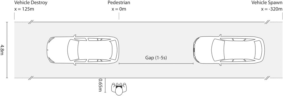
FIGURE 1. Schematic sketch of the experimental setup. The virtual vehicles appear at a distance of 320 m on a 4.8 m wide road, pass by the subject at a predefined speed and distance, and disappear at the end of the road.

The aim of this study is to evaluate a low-cost alternative to current, commonly applied approaches in pedestrian simulators such as consumer grade desktop-based VR HMDs and CAVEs as well as more recent approaches like AR. A simple Cardboard casing was used, without any padding. To limit discomfort while wearing the Cardboard, the duration of exposure to VR was minimized as far as possible. However, the aim was for the experiment to resemble the previous experiments as far as possible. Balancing these two objectives led to the following modifications compared to Maruhn et al. (2020) and Schneider et al. (2021): The number of trials was halved, and each combination of speed and gap size was presented once instead of twice. On the test track, the vehicles had to turn around after each run, drive back to the starting point and reposition themselves. However as in Maruhn et al. (2020), these waiting times were eliminated here. The vehicles disappeared at the end of the virtual road before being re-spawned at the starting point. Before starting their experiment, Maruhn et al. (2020) and Schneider and Bengler (2020) checked visual acuity using a simple paper-based test and determined each individual’s walking speed for the subsequent purpose of calculating safety margins. However, this was omitted in the present study as it was impractical in a remote setting in which there was no experimenter.

The overall experiment lasted about 30 min, including about 10 min of VR exposure. The study design was approved by the university’s ethics committee.

2.2 Apparatus

Participants of both Cardboard conditions were provided with an unassembled Google Cardboard along with instructions and with a QR code for installing the mobile application. Participants were encouraged to install the application on their own smartphone. Participants under the lab condition who did not have their own Android smartphone were provided with a Nexus 5 device.

2.2.1 Cardboard Viewer

A Google Cardboard version 2.0 was used for this experiment (cf. Figure 2A). By pressing a button on the upper right of the Cardboard causes a pillowed hammer covered with conductive strip to be pressed against the smartphone display (Linowes and Schoen, 2016). This enables button presses can be registered as touch events. The Cardboard has two lenses (∅ 37.0 mm). It weighs 140g, has the dimensions (145 × 87 × 87 mm), and supports smartphone display sizes of between 3.7” and 6” (9.4–15.2 cm). The originally introduced Google Cardboards (2015) claimed to have a Field of View (FoV) of 80° and a lens diameter of ∅ 34.0 mm (Linowes and Schoen, 2016) in comparison to 85° in AR (Maruhn et al., 2020) and 110° in the HMD (Schneider et al., 2021). The Cardboard has a printed QR code, which the test persons were asked to scan before they started. This adapts the display to the lenses and dimension parameters of the device [cf. Linowes and Schoen (2016)]. Neither the distance to the display nor between the lenses are adjustable. The Cardboard can be worn hands-free using an adjustable elastic headband. In practice, however, the use of a headband is not recommended. Holding the Cardboard with the hands limits the head’s rotation speed, which can prevent kinetosis (Linowes and Schoen, 2016). But as only a few rotations were to be expected in the present study design, mainly when the vehicles pass by, and as no interaction with the button on the Cardboard was necessary while waiting for the vehicles, the subjects were still provided with a headband. However, the participants were free to decide whether to use it (no instructions were provided for the headband) or to hold the Cardboard in place with their hands.

FIGURE 2

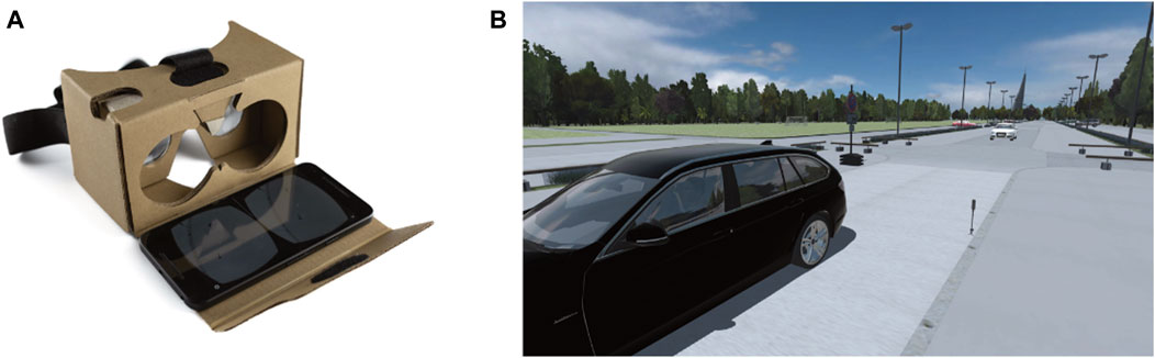
FIGURE 2. (A) Google Cardboard Version 2.0 Viewer with a Google Nexis 5 Smartphone. (B) View from the subject’s perspective during the experiment. Shown here is a 3-second gap at 30 km/h.

2.2.2 Mobile Application

The virtual environment from Maruhn et al. (2020) and Schneider et al. (2021) was transferred to an Android app (cf. Figure 2B), and the virtual environment was created in Unity 2019.3 and Google VR SDK 2.0. The experimental data was stored in an online database (Google Firebase). The app was distributed via Google Play Store.

On running the app, users stated whether they were working under the CBLab or the CBRemote conditions. They then had to confirm the subject information and informed consent. Users were asked to scan the QR code on the Cardboard. Since difficulties were observed when assembling the Cardboard under the lab condition, an explanatory stop motion animation was added for use under the remote condition. Finally, users entered their body height and the app switched to Cardboard mode. The virtual camera height was then adjusted to the subject’s body height. To reduce the number of draw calls and thus increase the performance, the virtual parking lot environment was converted into a 360° image from this camera position. This meant that no translational movements were possible (however, only rotations can currently be reliably tracked in Cardboards anyway). The two vehicles remaining as the sole dynamic objects featured 3D spatial sound. Upon entering the virtual environment, text boxes were displayed to introduce participants to the experimental task.

2.3 Experimental Task

Participants were told that they could interact with the virtual buttons in the VR by pressing the physical button in the Cardboard and using a gaze pointer to select a virtual button. The gaze pointer is a small white circle in the middle of the screen, that is only visible while the instructions are being displayed. The subjects were informed that the two vehicles would always approach from the right, with a constant gap and speed. Participants were asked whether they were standing and using headphones for audio output. They were asked to rate only the gap between the two vehicles in terms of whether they considered it safe to cross the road. If so, they were asked to signal their intention to cross the street at the moment that they would commence crossing. Since it was not possible to cross the actual test track for safety reasons, only the intention to cross was assessed. In Maruhn et al. (2020) and Schneider et al. (2021), this was signaled by taking a step forward towards the street. Since it is not possible to reliably track translational movements with Cardboards, this was signaled by pressing a button at the upper right of the Cardboard in the present study. Each press of the button caused an audible beep sound to be emitted. Each button press was recorded in the online database to calculate the objective measurements.

2.4 Objective Measures

Crossing initiation time (CIT) and gap acceptance were recorded as objective dependent measures. Gap acceptance was recorded as a dichotomous measure, indicating whether or not participants deemed a gap large enough to cross. If a participant decided to cross, the CIT was also calculated. CIT describes the time difference from the moment the first vehicle has passed until the subject presses the button. A negative CIT thus means that a crossing was initiated before the preceding vehicle had completely passed by the subject. A button press such as the one shown in the situation in Figure 1 would thus result in a CIT of 0s.

2.5 Subjective Questionnaires

After the trials were completed, the subjective data was recorded using the questionnaires contained in the app and results were also stored in the online database. The questions were the same as in Maruhn et al. (2020) and Schneider et al. (2021) and concerned demographics, how subjects rated the situations in which they did or did not cross the road, how easy they found it to make the decisions, and how likely it was that a collision would have occurred. The exact wordings can be found in Figure 10.

Online surveys or crowd-sourced data are often deemed to produce a low data quality as a result of careless behavior (Brühlmann et al., 2020). In long questionnaires, for example, attention checks are often used to identify deficient data sets. In this study, however, the focus was not only on the quality of the questionnaire but also on that of the simulator data. Another way of identifying careless behavior is to use self-reported single item (SRSI) indicators (Meade and Craig, 2012). At the end, participants were asked the following question, adapted from Meade and Craig (2012), using a continuous slider (extrema labels No–Yes): “It is critical for our study to include data only from individuals who give their full attention to this study. Otherwise, years of effort (by the researchers and other participants’ time) could be wasted. Hand on heart, should we use your data for our analyses in this study?”

2.6 Recruitment

Members of the university (staff and students) were recruited as subjects. They were approached spontaneously on campus, largely without any personal connection. However, this led to considerable data collection problems in the remote setting. To ensure anonymity, no contact information was collected from the participants. They were only provided with the Cardboard and printed instructions on how to install the app. An email contact address was provided in case of any further questions. However, data from the first subjects recruited in this way were for the most part never received. Technical reasons can be excluded here, as continuous monitoring of the app did not indicate any problems. It appeared to be down to a lack of incentive or commitment resulting from the complete anonymity. To circumvent this problem, participants whose contact data was available from the extended social environment of employees and students were recruited for the remote component. One week after the Cardboards were given out, a reminder was sent to the subjects to perform the experiment at home. However, the experimental data remained anonymous. Subjects were only allowed to participate if they had not taken part in a previous study by Maruhn et al. (2020) and Schneider et al. (2021).

2.7 Study Population

Thirty subjects completed the experiment in each of the two test environments CBLab and CBRemote. Male and female participants were equally represented in both settings. The age distributions under the laboratory condition (M = 26.53,  SD = 3.15, N = 30) and under the remote condition (M = 29.13,  SD = 3.60, N = 30) were comparable to the data previously collected in reality (M = 27.50,  SD = 2.08, N = 30), CAVE (M = 27.93,  SD = 3.42, N = 30), HMD (M = 27.73,  SD = 3.00, N = 30), and AR (M = 27.62,  SD = 3.55, N = 13). Although the idea was to be able to recruit more diverse samples for the Cardboards used in a remote setting, this was not done here on grounds of comparability.

2.8 Hardware Performance

The current frame rate, measured in frames per second (fps), was continuously tracked during the trials. So as not to affect the performance, the frame rate was measured with a frequency of 4 Hz. The number of frames was divided by the elapsed time, i.e., the average frame rate of the previous 250 ms. The minimum and maximum frame rates were then logged for each trial. The phone’s display resolution was also logged. The results are presented in Figure 3. Overall, the smartphones used under the remote condition were higher performing. The minimum frame rates measured (Figure 3A) are in many cases well below the frequently recommended level of 60fps (CBLab: M = 25.84fps,  SD = 14.09fps, CBRemote: M = 31.85fps,  SD = 13.29fps). However, it should be noted that these minimum frame rates usually only occur for a very short time, for instance, during a rapid head movement or when rendering complex 3D objects. Unfortunately, this generally happens when the vehicles are going past the test persons, who follow the vehicle movements with their heads. It can therefore not be completely ruled out that it affects the estimation task. In many smartphones, the maximum frame rate is limited to 60 fps (Linowes and Schoen, 2016), or even lower values, particularly in older models. The smartphones used under the remote condition achieved slightly higher maximum frame rates (M = 57.66fps,  SD = 4.59fps) than those in the laboratory (M = 52.90fps,  SD = 9.70fps), see Figure 3B. Regarding the display resolutions, only minimal differences between the smartphones used in the lab (M = 2.15 MP,  SD = 0.62 MP) and those employed at home (M = 2.03 MP,  SD = 0.47 MP) can be determined (Figure 3C).

FIGURE 3

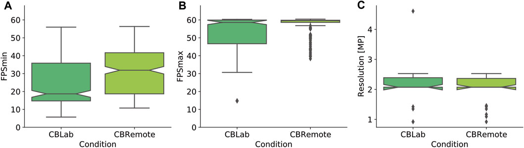
FIGURE 3. Hardware performance indicators for the smartphones used in the two test environments. (A) shows the minimum frame rates that occurred in the test runs, and (B) the maximum frame rates achieved. (C) compares the display resolutions.

2.9 Data Exclusion

If participants wished to mark a trial response as erroneous, for example, if they had clicked by mistake, they were asked to signal this by pressing the button three times. However, this did not happen in any of the trials. But there were several occasions on which a button was pressed well before or after the vehicles had passed. These cases were then deleted (CBLab: 2, CBRemote: 1). A CIT of ± 20s was defined as the threshold value. After this cleanup, a number of duplicate button presses still remained. In such cases (CBLab: 2, CBRemote: 8), the first of the two button presses was used in the onward analysis. Subsequently, there still remained cases in which the CIT was larger than the actual vehicle gap. Furthermore, very late button presses, i.e., those made shortly before the second vehicle passes cannot be considered as representing a time to start crossing. Consequently, CITs larger than half the gap size were excluded (CBLab: 2, CBRemote: 19) in CIT comparisons and only considered as gap acceptance. Under the laboratory condition, these data points were distributed among six subjects, and under the remote condition, among 13 subjects. It is possible that several of these excluded data points might occur for one subject. There was one participant in the remote group for whom five cases of double button presses occurred accompanied by five cases with excessively large CITs. This subject also accepted every gap. However, the cleaned data seemed plausible. Accordingly, it cannot be ruled out that the subject actually found all gaps passable and that the instructions had not been misunderstood. This subject was therefore not excluded from the analysis. The other cases were evenly distributed among the test subjects. Overall, more data points had to be cleaned under the remote condition than in the laboratory.

2.10 Data Analysis

Null hypothesis significance testing (NHST) is the predominant method of data evaluation used in human factors research, which includes driving simulator studies (Körber et al., 2016), although it does have some limitations and problems. NHST is often used to render a dichotomous statement, such as “Does an independent, manipulated variable have a significant effect on a dependent, observed variable?” This decision is then usually based on a previously defined α error level. The p value of a frequentist test indicates how likely the observation was, assuming the manipulated variable has no influence. However, the p value depends on a number of factors that must be taken into account by the researcher, such as sampling stopping rules and test selection (Kruschke, 2015a). Besides this single point estimate in the form of a p value, plausible limits around this estimator, i.e., confidence intervals, are also increasingly used in the social and behavioral sciences (Cumming and Finch, 2001). However, since confidence intervals are based on the same assumptions as p values, they suffer from the same limitations as those described above (Kruschke, 2015a). Moreover, confidence intervals only provide bounds, not a distribution function of the estimator (Kruschke, 2015a). This is in contrast with Bayesian statistics. Here, the outcome is actually a distribution function of the estimator. Bayesian approaches also avoid approximation assumptions (Kruschke, 2015b, p. 722) and allow for equivalence testing. These and other benefits have led to a rapid rise of Bayes methods in a variety of disciplines (Kruschke et al., 2012), but not in social and behavioral research [e.g. Kruschke et al. (2012); Körber et al. (2016)]. This work is a first step in applying Bayes statistics in the context of pedestrian simulator studies. Data analysis and model creation for this work were performed in Python, version 3.8.

3 Results

As stated at the beginning of this work, this study replicates a design that has already been performed in reality, as well as in CAVE, HMD (Schneider et al., 2021), and AR (Maruhn et al., 2020). To better understand the results of this work in the overall context (Research Question 1), the data from previous studies are given in figures and analyses. The number of trials in the present setting was half that used in previous studies, and each combination of gap size and speed was presented only once. Accordingly, only the first 10 trials from the previous studies were considered. The data analysis focuses on two comparisons: the difference compared to the test track and the difference between the two Cardboard conditions (laboratory and remote, Research Question 2).

3.1 Gap Acceptance

In addition to the 300 crossings (10 trials x 30 participants) performed under each of the two Cardboard conditions (lab and remote), the analysis also includes crossings made in previous studies: REAL (300), CAVE (300), HMD (298, whereby 2 data points were excluded because the subjects were too far in front of the virtual light barriers) and AR (130, as there were only 13 subjects). Figure 4 presents a summary of acceptance rates isolated for the variables: test environment (Figure 4C), gap size (Figure 4D), and speed (Figure 4E), as well as the combination of test environment and gaps (Figures 4A,B). In total, 654 of the 1,628 crossing opportunities were rated as passable, representing an acceptance rate of 40%. Acceptance rates for each factor were calculated from combinations of the remaining two factors (cf. Figure 4). Acceptance rates were highest in the real environment on the test track (M = 0.48,  SD = 0.5) followed by CAVE (M = 0.43,  SD = 0.5), CBRemote (M = 0.42,  SD = 0.49), CBLab (M = 0.39,  SD = 0.49), HMD (M = 0.34,  SD = 0.47), and AR (M = 0.28,  SD = 0.45). More gaps were accepted overall at 50 km/h (M = 0.43,  SD = 0.5) than at 30 km/h (M = 0.37,  SD = 0.48).

FIGURE 4

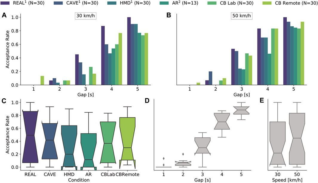
FIGURE 4. Descriptive data of gap acceptance rates. (A,B) show the acceptance rates as a combination of vehicle gap and test environment subdivided for both levels of speed. The bottom three plots each represent one independent variable in isolation. The acceptance rates are shown as a function of (C) the experimental environment, (D) the gap sizes and (E) the levels of speed. The box plots show the distributions based on the other two respective factors. For example, (D) shows that there are combinations of test environment and speed that lead to a gap acceptance of 0 at 3s. In (A) it can be seen that these are AR at 30 km/h. The experimental data in REAL, CAVE and HMD were collected in Schneider et al. (2021). The experimental data in AR were collected in Maruhn et al. (2020).

A mixed logistic regression model was generated to analyze the binary outcome of gap acceptance. The gap sizes were re-centered around 0 to accelerate data processing and simplify model interpretation. To account for this, the factor gap size is referred to as GapC in the model descriptions and summaries. The base model included condition (categorical, 6 levels: REAL, CAVE, HMD, AR, CBLab and CBRremote), speed (categorical, 2 levels: 30 and 50 km/h), gap size centered (continuous, 5 levels: −2, −1, 0, 1, and 2s) and participant as a random factor (ID). The REAL condition served as a baseline. Speed was treated as a categorical variable, since only two velocities were used in the experiment. Two additional models were created by adding random slopes for either gap size or speed as was one more model, in which two fold interactions of the condition with the speed and gap were added to the base model. The models were created with Bambi (Capretto et al., 2020) which is built on top of PyMC3 (Salvatier et al., 2016). Bambi allows for formula-based model specification and automatically generates weakly informative priors (Capretto et al., 2020). The Hamiltonian Monte Carlo algorithm in combination with No-U-Turn Sampler (Homan and Gelman, 2014) is then used to compute the posterior distribution depending on the priors and the likelihood function of the observed data. Each model was created with 4,000 draws and 4 parallel chains. The target accept (sampler step size) was increased to 0.99 to remove any divergences, especially in the more complex model with interactions. ArviZ (Kumar et al., 2019) was used to analyze and compare the Bayesian models created. The results are shown in Table 1. Despite being only ranked second, the base model will be used for further data analysis. Since there is only a marginal difference in the information criterion (loo: leave-one-out cross validation), the base model was chosen due to its simpler model complexity and parameter interpretation. The structure of the base model is illustrated in Figure 5 as a distogram, according to the convention by Kruschke (2015b). The model’s output is summarized in Table 2. No divergences occurred in the model. For none of the fixed effects did a rank normalized R-hat $\widehat{R}>1.00$ occur [cf. Vehtari et al. (2021)]. Visual inspection of the trace plots indicated a sufficient exploration of the parameter space and mixing of the chains.

TABLE 1

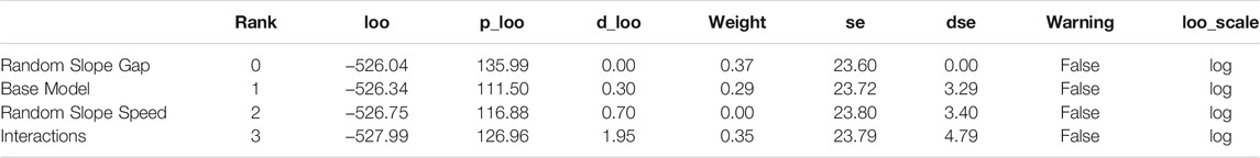
TABLE 1. Model comparison for predicting crossings as a function of condition, gap size, and speed as fixed factors and participant as a random factor. In addition to this base model, the other models include either a random slope for gap or speed, while one model features two-way interactions of gap and speed with condition.

FIGURE 5

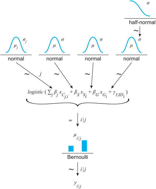
FIGURE 5. Model structure for predicting each binary outcome of a possible crossing (y_i) depending on the simulation environment (j) and based on a Bernoulli distribution. Its μ value results from a linear logistic function with condition (C, 6 categorical levels referenced by index (j), speed (S) and gap size (G) as fixed effects. Due to the repeated measures design, the participants’ ID was treated as a random effect (γ). The estimators were assigned weakly informative priors: normal distribution for the fixed effects and half-normal for the σ of the normal distribution for the random effect.

TABLE 2

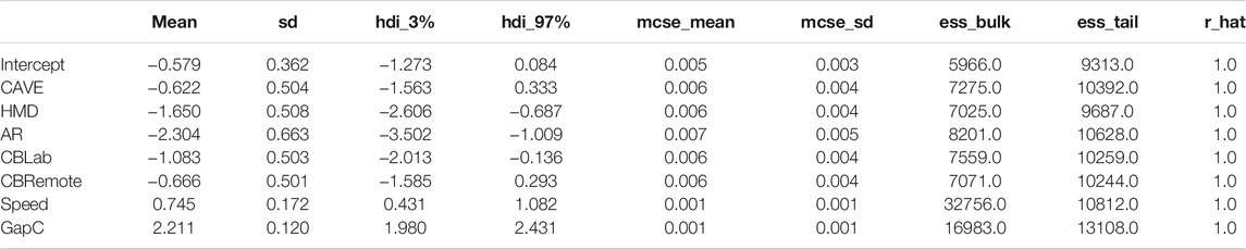
TABLE 2. Summary for crossing model: Crossing ∼ Condition + Speed + GapC +(1|ID). REAL served as a baseline. GapC refers to the centered gap size variable [−2s, 2s] rather than [1s, 5s].

Contrary to NHST, Bayes analysis provides a distribution of estimators instead of a point estimate. The further analyses are limited to the estimators for the different conditions. If the beta estimators for condition are considered in isolation, this corresponds to a model equation in which Gap x_S and Speed x_G are set equal to zero (cf. Figure 5). Since Gap was re-centered, this corresponds to an estimate for 3s gaps at 30 km/h (baseline speed). The distributions of the beta estimators for the different conditions can be subtracted from each other. For example, if the CBLab distribution is subtracted from the CBRemote distribution, a conclusion can be drawn about how the estimation for a crossing differs between the two conditions relative to the REAL condition. The result of a linear combination from a logistic regression are given in logits. By applying an exponential function, the logits can be converted to odds. Dividing the odds by 1 + odds results in probabilities (Equation 1).

$probability=\frac{e^{logit}}{1+e^{logit}}(1)$

Of particular interest are the differences in the crossing probabilities between the simulators and reality (Research Question 1) as well as between the two Cardboard conditions (Research Question 2). Figure 6 contrasts these differences in a ridge plot. The plot shows the respective posterior distributions’ 94% highest density interval (HDI). HDIs are often given as 94% to emphasize their difference to confidence intervals. As with classical NHST, there are now several ways of describing the magnitude of these differences and, in contrast to NHST, about their equivalence as well (Kruschke, 2015b, p. 335 ff.). One way is to define a region of practical equivalence (ROPE). The boundaries of this region can be specified individually, depending on the use case. In this work, a data-driven approach was chosen. Kruschke (2018) defines ROPEs based on the population standard deviation and half the size of a small effect (δ = ±0.1) according to Cohen (1988). Since no standard deviation of the population is available in the present case, the sample standard deviation is used. With a dichotomous outcome variable, no standard deviation can be calculated initially. However, since each subject (i) repeated the experiment 10 times, the mean crossing probability of each subject (${\widehat{p}}_i$ = accepted crossings/number of repetitions) and the mean crossing probability of all subjects (${\widehat{p}}_0$) can be used to calculate the standard deviation of the crossing decisions of all participants (Eq. 2). The ROPE limits were then defined by multiplying σ_crossing by ± 0.1 (Eq. 3). This results in a ROPE of ±0.018. Thus, differences of ±1.8% are treated as practically equivalent.

${\sigma }_{crossing}=\sqrt{\frac{{\mathrm{\Sigma }}_{i=1}^N{({\widehat{p}}_i-{\widehat{p}}_0)}^2}{N-1}}(2)$

$ROPE=\pm 0.1\ast {\sigma }_{crossing}(3)$

FIGURE 6

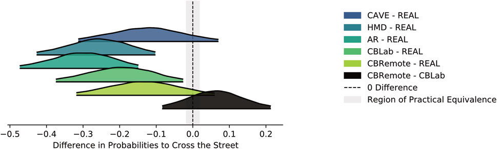
FIGURE 6. Difference in posterior probabilities of crossing the street (for a 3s gap and at 30 km/h) between the simulators and the real-world setting, and between the two Cardboard settings.

As can be seen in Figure 6, the combination of weakly informative priors and a relatively small set of data points results in very broad distributions relative to a narrowly defined ROPE. Accordingly, none of the distributions lies entirely within the ROPE and no practical equivalence can be assumed for any of the comparisons. The HDIs of HMD-REAL (HDI [ − 0.426, −0.103]), AR-REAL (HDI [0.472, −0.149]) and CBLab-REAL (HDI [− 0.374, −0.026]) are completely outside the ROPE. Fewer gaps are accepted in these conditions than on the test track. For the remaining comparisons CAVE-REAL (HDI [− 0.313, 0.069]), CBRemote-REAL (HDI [− 0.318, 0.059]) and CBRemote-CBLab (HDI [− 0.083, 0.213]), no statement can be made, because they are neither completely enclosed by the ROPE nor completely outside the ROPE. Makowski et al. (2019) describe another way of defining ROPEs for logistic models. For completeness, the evaluation is included in the analysis script provided online.

$ROPE=\pm 0.1\ast \frac{\pi }{\sqrt{3}}(4)$

They propose converting the parameters from log odds ratio to standardized difference using Eq. 4, resulting in a ROPE of ±0.181 on the logit scale. This approach yields the same results in this context, except that the CBLab-REAL comparison is just no longer completely outside the ROPE.

3.2 Crossing Initiation

Of the 654 gaps accepted, CITs were calculated for 633 deemed as potential crossings. Twenty-one cases were dismissed for which the CIT was greater than half the gap size (cf. Section 2.9). Since gap acceptance rates varied between the test conditions, so did the number of CITs: REAL (N = 145), CAVE (N = 128), HMD (N = 101), AR (N = 37), CBLab (N = 114) and CBRemote (N = 108). The overall mean CIT was 0.16s (SD = 0.52s), whereas in REAL (M = −0.27s,  SD = 0.45s), distinctly lower CITs were observed than in the simulators: CAVE (M = 0.35s,  SD = 0.51s), HMD (M = 0.16s,  SD = 0.47s), AR (M = 0.38s,  SD = 0.46s), CBLab (M = 0.24s,  SD = 0.34s) and CBRemote (M = 0.34s,  SD = 0.49s). As the gap size increased, CITs also increased slightly: 2s (M = −0.04s,  SD = 0.48s), 3s (M = 0.06s,  SD = 0.47s), 4s (M = 0.15s,  SD = 0.52s) and 5s (M = 0.21s,  SD = 0.52s). At 30 km/h, participants made the decision to cross earlier (M = 0.03s,  SD = 0.55s) than at 50 km/h (M = 0.26s,  SD = 0.46s). Figure 7 shows the CITs as a function of condition (Figure 4C), gap (Figure 4D), speed (Figure 4E) or a combination of condition and gap for the two levels of speed (Figure 4A and Figure 4B).

FIGURE 7

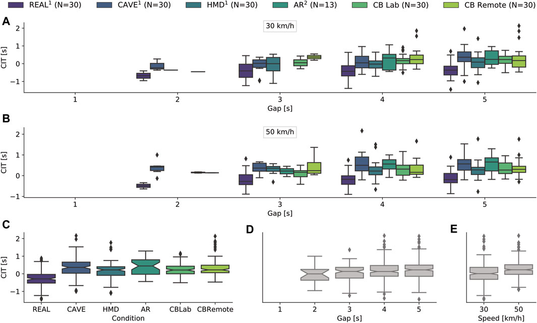
FIGURE 7. Descriptive data of crossing initiation times (CIT). (A) and (B) show CITs as a combination of vehicle gap and test environment, subdivided for both levels of speed. The bottom three plots each represent a single independent variable. The CIT is shown as a function of (C) the experimental environment, (D) the gap sizes and (E) the speed levels. The experimental data in REAL, CAVE and HMD were collected in Schneider et al. (2021). The experimental data in AR were collected in Maruhn et al. (2020).

In a similar way to the gap acceptance analysis above (cf. Section 3.1), different models were created with which to predict CITs. Again, the base model featured condition, speed, gap size centered (GapC) plus the participant as a random factor (ID), while the additional models included either interactions or random slopes. The loo values for the models were again very similar, and therefore, the simple base model was chosen. The exact values can be found in the accompanying data analysis script. It should be noted that warnings appeared in the course of the model comparison [based on loo using Pareto-smoothed importance sampling (Vehtari et al., 2017)] to the effect that the estimated shape parameter of Pareto distribution was greater than 0.7 for some observations. Observations where κ > 0.7 indicate influential data points, and errors in loo estimation (Vehtari et al., 2017). Further analysis of these data points revealed that they are extreme values under the CAVE (N = 6), HMD (N = 6), and CBRemote (N = 3) conditions with comparatively very low or very high CITs. However, since the data points represent plausible CITs, they are not excluded from the model. The visual inspection of trace plots and auto-correlation plots, as well as the posterior predictive checks and the absence of divergences otherwise imply a sufficient model fit. The resulting model summary is presented in Table 3 and the model schema is shown in Figure 8.

TABLE 3

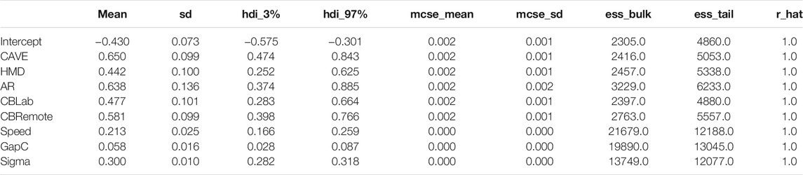
TABLE 3. Summary for CIT model: CIT ∼ Condition + Speed + GapC + (1|ID). REAL served as a baseline. GapC refers to the centered gap size variable [−2s, 2s] rather than [1s, 5s].

FIGURE 8

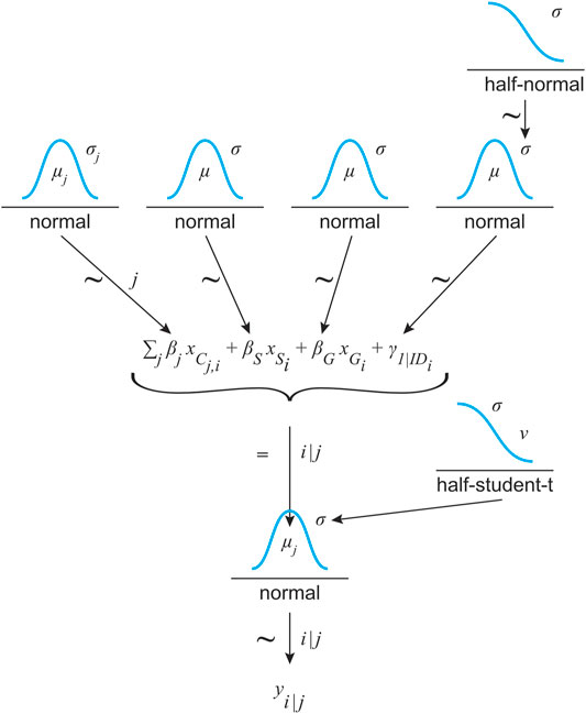
FIGURE 8. Model structure for predicting CIT (y_i) depending on the simulation environment (j) and based on a Gaussian distribution. Its μ value results from a linear function with condition (C, 6 categorical levels referenced by index (j), speed (S) and gap size (G) as fixed effects. The standard deviation of the Gaussian distribution σ is estimated on the basis of a weakly informative normal prior distribution. Due to the repeated measures design, the participants’ ID was treated as a random effect (γ). The estimators were assigned weakly informative priors: normal distribution for the fixed effects and half-normal for the σ of the normal distribution for the random effect.

Here, too, further analysis focuses on the differences in the CITs between the simulation environments and reality and on comparing the two Cardboard conditions. The ROPE was determined on the basis of the standard deviation of all CITs as ± 0.1*σ_CIT. Based on σ_CIT = 0.52s, this results in a ROPE of ±0.052s. Figure 9 plots the difference in posterior distributions. Compared to the test track, the participants indicated their crossing decisions later in all simulated environments: CAVE-REAL (HDI [0.474, 0.843]), HMD-REAL (HDI [0.252, 0.625]), AR-REAL (HDI [0.374, 0.885]), CBLab-REAL (HDI [0.283, 0.664]), CBRemote-REAL (HDI [0.398, 0.766]). No statement can be made regarding a practical equivalence for the comparison between CBRemote and CBLab (HDI [ − 0.090, 0.300]).

FIGURE 9

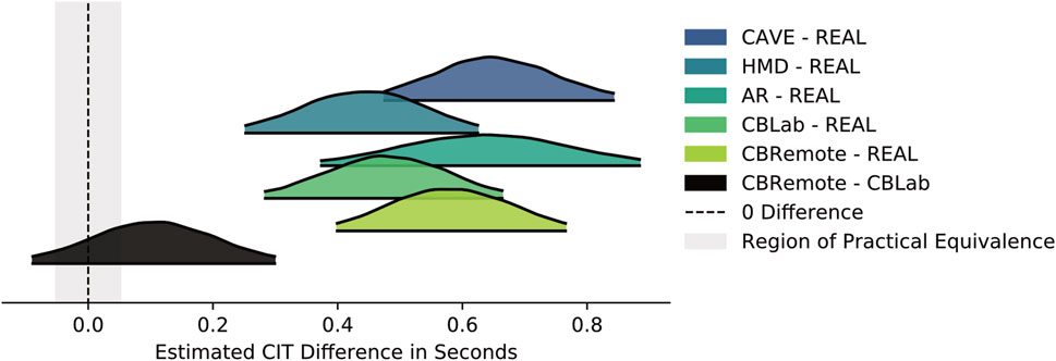
FIGURE 9. Difference in posterior estimates for CIT (for a 3s gap and at 30 km/h) between the simulators and the real setting, and between the two Cardboard settings.

3.3 Subjective Data

Figure 10 presents all the questionnaire’s results along with the wordings of the questions. Table 4 gives an overview of means and standard deviations for each item and experimental setting. Overall, participants rated it quite safe to cross the street (Q1, Likert scale [1, 4]), with the highest scores achieved in reality on the test track, followed by AR, CBRemote, HMD, CAVE and CBLab. Collisions (Q2, Likert scale [1, 4]) were assessed as somewhat unlikely with the lowest values in AR, followed by CBRemote, REAL, CBLab, HMD and CAVE. The severity of collisions (Q3, Likert scale [1, 4]) was rated highest in AR followed by CBLab, REAL, CBRemote, HMD and CAVE. The two questions on similarity of behavior compared to reality (Q4 and Q5, continuous scale) were normalized to obtain values between 0 and 1. Both questions produced similar results. In cases in which the participants crossed the street, behavior was rated the most similar in CBRemote followed by REAL, HMD, AR, CAVE, and CBLab. Again, in cases in which they did not cross, CBRemote scored highest, followed by CAVE, HMD, REAL, CBLab, and AR. This high correspondence to real road traffic situations was also reflected in the following question. The subjects indicated that their decisions were neither particularly safe nor unsafe compared to other situations (Q6, Likert scale [−2, 2]). Deciding to cross the street (Q7, Likert scale [−2,2]) was more difficult than usual, with the highest scores obtained in AR, followed by CBLab, CBRemote, HMD, REAL and CAVE. The participants also reported that taking this decision took longer (Q8, Likert scale [−2, 2]), being the shortest in CBLab, followed by CAVE, REAL, AR and CBRemote, and the longest in HMD.

FIGURE 10

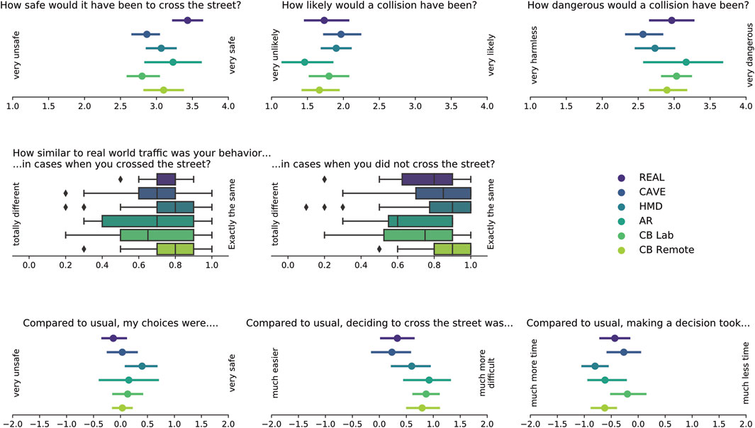
FIGURE 10. Descriptive data from the questionnaires. Questions with Likert response scales are represented by point plots, questions with continuous response scales by box plots. For the Likert-scaled items, only the most extreme response options are indicated at the edges of the X axis in each case.

TABLE 4

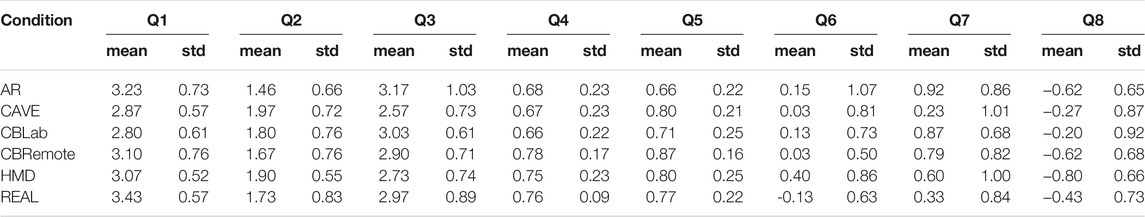
TABLE 4. Summary of questionnaire data. See Figure 10 for questions wordings.

Again, a Bayesian approach was chosen for analysis. For each question, a separate model was set up and fitted. In all models, the test environment served as the fixed (and only) factor, with REAL as the baseline. Likert-scaled items (Q1–3 and Q6–8, cf. Figure 10) were evaluated using ordered logistic regression. Since Bambi (Capretto et al., 2020) does not support ordered logistic regression at the time of writing, it was modeled in PYMC3 (Salvatier et al., 2016). Following McElreath (2020, Chapter 12) and consistent with previous analysis in this paper, weakly informative priors were used. Visual inspection of trace and auto-correlation plots indicated sufficient sampling, and posterior predictive plots evidenced an adequate fitting of the separate models. The two questions with continuous response scales were fitted with Bambi. Again, the test environment served as the sole factor. Here, posterior predictive checks indicated a poor fit between the Gaussian model and the heavily left-skewed data (cf. Figure 10). Data with a range from 0 to 1 was mirrored at 0.5 to obtain a right-skewed distribution and fitted to a Gamma distribution with log link functions to avoid divergences appearing with canonical link functions. Since these distributions do not support the observed values of 0, 1e − 5 was added to these data points. Ideally a truncated distribution that accounts for left-skewed data should be used. However, none is available at the current state of the libraries used. For both questions and the respective models, a model comparison revealed a higher model fit (based on loo values) for the Gamma models. However, the Gamma model for Q4 resulted in implausible posterior distributions under HMD and CBRemote conditions. The Gaussian model was therefore applied. Differences in posterior distributions were calculated to enable comparison of the two Cardboard conditions.

Similar to Figures 6, 9, 11 shows the differences in estimator distributions for the above mentioned comparisons for each question. The outputs for the Likert-scaled items (Q1–3 and Q6–8) are displayed in logits, the results of Q4 on a log scale. In the case of logits, the ROPEs are defined by Eq. 4. The ROPEs’ limits for the continuous items (Q4 and Q5) are again data driven and defined by the standard deviation of each response item: ±0.1*σ_{Question−Item} respectively ±0.1*σ_{log(Question−Item)} to account for the Gamma model’s log link function.

FIGURE 11

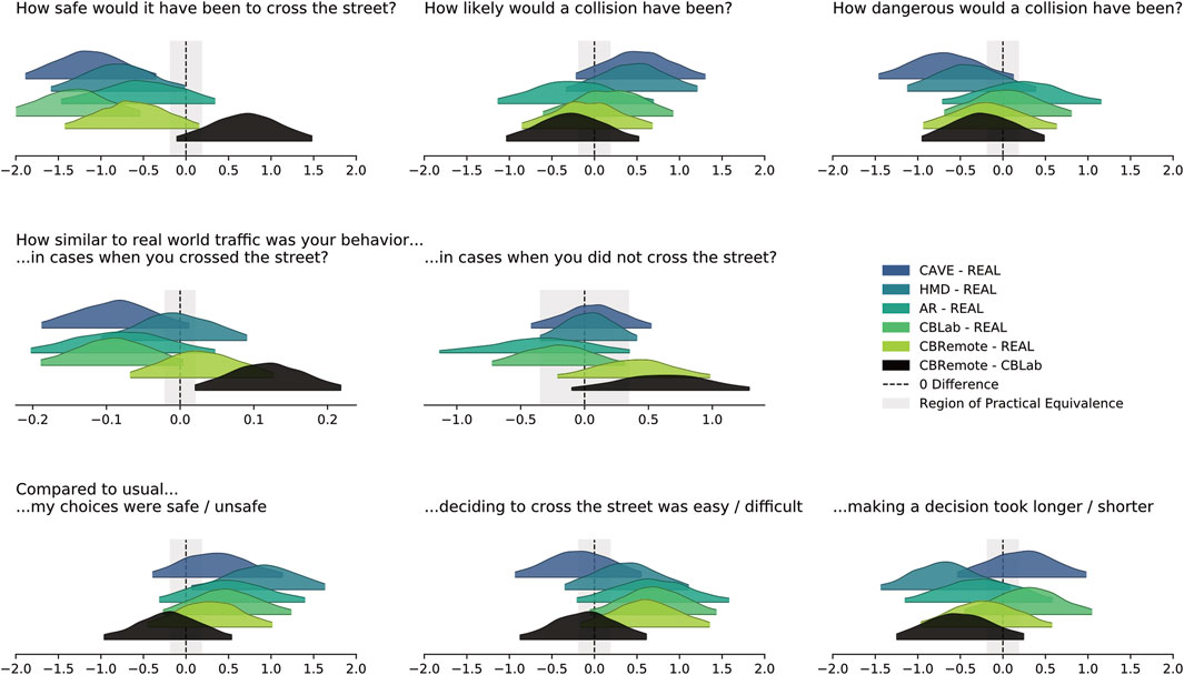
FIGURE 11. Difference in posterior estimates for each of the subjective items in the questionnaire (cf. Figure 10). The results for Q1-3 and Q6-8 in the upper and lower rows are given in logits, the results of Q5 in the center plot on a log scale.

Crossings in CAVE (HDI [ −1.886, −0.353]) and CBLab (HDI [−2.119, −0.539]) were rated unsafer than REAL based on a ROPE with the limits [−0.181, 0.181]. The results for HMD-REAL (HDI [−1.585, −0.013]), AR-REAL (HDI [−1.468, 0.340]), CBRemote-REAL (HDI [−1.419, 0.155]) and between the Cardboard conditions CBRemote-CBLab (HDI [−0.111, 1.481]) were inconclusive. Regarding ratings of how likely a collision would have been, neither differences nor equalities could be reported. The same applies to the questions relating to how dangerous a collision would have been. In cases in which the participants decided to cross, the behavior was rated closer to the real world traffic (HDI [0.020, 0.218]) under the remote Cardboard condition compared to the Cardboard under lab conditions based on ROPE with limits [−0.020, 0.020]. A similar trend could be observed in those cases when it was decided not to cross the street. The results regarding how safe or unsafe the choices were are also inconclusive, although participants tended to rate their crossings safer with the HMD than with REAL (HDI [0.066, 1.631]). Likewise, the results for the last two questions are inconclusive: i.e., 1) rating the decision as to whether to cross the street as easy/difficult and 2) how long it took to make the decision.

Finally, participants under the two Cardboard conditions were asked to rate the quality of their experimental data (SRSI, cf. Section 2.5) on a scale from 0 to 100. Under both conditions, the ratings were comparatively high: CBLab M = 96.57,  SD = 5.16, CBRemote M = 97.25,  SD = 5.73. The overall minimum was 74.88. Again, the distributions were left-skewed and thus mirrored and fitted with a Gamma distribution with log links (again to avoid divergences) and with the test environment as the only factor. The Gamma model performed better (loo = 159.45,  SE = 45.22) showing a great improvement compared to the Gaussian base model (loo = −178.24,  SE = 10.79). Again, 1e − 5 was added to values of 0 to allow the Gamma distribution to be fitted. The ROPE was again (cf. Q5) calculated based on the standard deviation of the observed, log transformed SRSI values. CBLab served as baseline in the model. The HDI for the effect of CBRemote compared to CBLab encompasses [−0.318, 0.281] and is thus completely within the ROPE ([−0.541, 0.541]).

4 Discussion

This research was carried out to answer two research questions, namely, whether low-cost Cardboard headsets are a suitable substitute for high-end pedestrian simulator hardware and, secondly, whether they can be used to conduct studies in a remote setting with no experimenter present.

4.1 Cardboards and Other Simulators

The results observed in terms of gap acceptance were relatively similar to those in the other high-end simulation environments. Here, the two Cardboard conditions rank between the Vive Pro HMD and CAVE. Compared to the high-end HMD, the subjects accepted more gaps with the Cardboards and the results were thus more similar to those on the test track. However, it should be critically mentioned that the mode of signaling a crossing decision differs between Cardboards and other data. Since no translations could be tracked, detecting a step in the direction of the road was not possible, unlike in the other conditions and was instead signaled by pressing a button. Schwebel et al. (2017b) compared Cardboard button presses versus taking a step in a kiosk environment and detected a correlation in the number of missed crossing opportunities but only a correlation trend for CITs. Further studies should investigate the differences between button presses and naturalistic walking so as to render older HMD studies (mostly involving button presses) comparable with newer settings and their larger tracking areas. The need for such methodological comparisons can be clearly seen by comparing the results from these studies with those from Mallaro et al. (2017). In a similar research question, Mallaro et al. (2017) reported that the gaps accepted in an HMD were smaller than with a CAVE. The experimental task may also have had an influence here. In contrast to the study design presented in this work, in Mallaro et al. (2017), the street was crossed by physically walking. A comparison of accepted gaps is also interesting: while the overall rate of acceptance of a 3s gap was 34% here, 3s gaps were accepted much less frequently in Mallaro et al. (2017). The question arises what influence the range of the presented gaps have on the test person. Even if only smaller gaps are presented, the participant might feel compelled to accept gaps that he or she would actually consider too small just to fulfill the experimental task or expectations. However, another reason could be that participants receive feedback when they actually walk, so they might not cross the next time if they know that the time was not enough in a previous trial. It should be noted that the participants cannot see their own bodies in the Cardboards of any form. This is, however, possible in REAL, CAVE and AR as well as with a virtual avatar in HMD, by means of trackers positioned on their extremities, but this is not immediately feasible using a phone-based approach. However, the representation of one’s own body seems to have an impact on the gap sizes accepted (Maruhn and Hurst, 2022).

Turning our attention to the CITs, the two Cardboard conditions fit in with the rest of the simulators. Particularly striking are the similarities of the two Cardboard distributions with the HMD distribution (cf. Figure 9). The Bayesian analysis confirmed that in all simulated environments, the crossing was initiated later than in the real-world setting on the test track. These results call into question the transfer of measured absolute values from simulation to reality [absolute validity, (Wynne et al., 2019)]. This is of particular relevance when determining safety-relevant measurements in road traffic, for example. Currently, this does not seem possible on the basis of virtual scenarios. The evaluation in Schneider et al. (2021) even questions relative validity: an influence of vehicle speed on gap acceptance could only be demonstrated in the two simulator environments (CAVE and HMD), but not on the test track (REAL). Not only the distorted distance perception in VR (Renner et al., 2013) but also the lack of resolution could still be a problem. Especially at large distances, the display of vehicles is reduced to a few pixels. Although this problem would be even more drastic under the Cardboard conditions, the differences in gap acceptance compared to the test track (Figure 6) and CIT (Figure 9) are similar to those in the other simulators. Other factors besides display resolution also seem to play a role.

Similarities were not only found with the objective data but also between Cardboards and the other simulators in the subjective ratings. In all simulators, participants indicated that it would have been less safe to cross the street than participants in REAL. This could explain why, overall, fewer crossings were accepted in the simulators and they were initiated later. The Bayesian analysis confirmed this difference for CAVE and CBLab. The fact that this was not confirmed for the remaining simulators is mainly due to the very broad distributions. There seems to be a trend that collisions were rated as being more likely to happen in CAVE and HMD but, at the same time, they would have been less dangerous. However, the results of the Bayes analysis do not allow for definitive differences. As for the first question, participants in all simulators rated their decisions as unsafer, even tough, this is only a trend. The participants seemed to have slightly greater problems making a decision with AR, HMD and the two Cardboard conditions, even though no definitive statements can be made. This can probably be seen as an effect of wearing an HMD.

4.2 Laboratory and Remote Setting

Approximately the same number of gaps were accepted under both Cardboard conditions with slightly more under the remote condition (cf. Figure 6), whereby the decisions were also taken slightly later (cf. Figure 9). However, the data quality from the remote setting must be viewed critically. More data points had to be treated than in the laboratory setting (cf. Section 2.9). The chosen criteria led to the exclusion of a large proportion of the implausible data, but some 1s gap acceptances from the remote setting remained (cf. Figure 4A). It was not certain whether a crossing was actually desired. For the evaluation of the CIT, however, these cases were excluded according to the defined rules. This is also one of the major disadvantages of a remote setting. Informal interviews after an experiment, which can help to check the plausibility of data, are no longer possible. Thus, it is not possible to determine in the remote condition whether the cause was misunderstood instructions, the uncontrolled setting, or, indeed, other effects.

Based on the Bayes analysis, no definitive conclusions can be drawn between the two Cardboard conditions regarding possible differences in objective measures. No differences occurred, but no practical equivalence could be demonstrated either. In particular, the combination of weakly informed priors, small amounts of data, and narrowly defined ROPEs meant that in none of the cases, neither for the objective nor for the subjective measures, does the ROPE completely enclose the distributions of differences between CBLab and CBRemote. Nevertheless, the results may be of value for future studies, for instance, for defining more informed priors or evaluating the data using other, practically dedicated, ROPEs.

While no data equivalences were demonstrated, there were some differences in the subjective measures. There seemed to be a trend that participants felt it was safer to cross the street in the remote setting. The differences between CBLab and CBRemote with the two continuous questionnaire items are worth highlighting. In both cases (when the participants crossed or did not cross the street), participants reported a high level of agreement with their everyday behavior, but this was even higher in the remote condition. Although no differences in objective data could be found, subjects in a home setting with no experimenter present seemed to subjectively perceive a higher degree of consistency with their everyday behavior. Even though more data points had to be treated in the remote setting (13 subjects vs 6 subjects in the lab), subjectively, participants rate their data quality as being equally high. Even if it was not subjectively perceived that way, the subjects may have performed the experiment with less accuracy or attention in the remote setting. It is also not possible to ensure whether participants in the remote setting were more distracted by external influences at home. Overall, however, it should be noted that the data in the two settings are very similar, and a remote setting can be considered comparable to a laboratory one and can even induce more subjectively realistic behavior. This again demonstrates how low cost, mobile-VR headsets can be seen as a suitable hardware device for experiencing virtual traffic scenes from a pedestrian perspective (Schwebel et al., 2017a; Schwebel et al., 2017b), even if it comes with some limitations.

5 Limitations and Implications

This work marks a first attempt at conducting pedestrian simulator studies in a remote setting. Naturally, there are also limitations. The young age group across all experiments does not allow a generalization of the results to children or older adults. However, limitation to one age group was necessary to control for inter-individual differences in this between-subjects design (Schneider et al., 2021). A within-subject design would have increased the statistical power, but this was not possible and could have induced new effects (learning effects, comparative judgments) and it can limit comparison with previously collected data. Many optimizations were made to achieve a sufficiently high frame rate on mobile devices, but this could not always be ensured. However, it can be assumed that smartphone performance and display resolution will continue to increase over the next few years and that even complex virtual environments can be displayed smoothly. In the future, additional cell phone sensors could enable reliable tracking of translational movements in addition to head rotation, enabling other forms of interaction than button presses. Some participants took the opportunity to provide feedback on the experiment in a text input field in the questionnaire. Five users said that the vehicles started off at too great a distance or that there was too much waiting time between trials. This was also the case in other environments, where the waiting time between trials was even longer, but the vehicles were discernible at greater distances. In contrast, the lower display resolution of some of the smartphones meant that vehicles were not even recognizable at their starting position. In order to minimize the discrepancies with the other studies, these waiting times were nevertheless included. Three participants stated that the image was slightly blurry. This could be due either to low screen resolution or to the presence of screen protectors. Another limitation in imaging is that the lens distance could not be adjusted to the individual interpupillary distance (IPD). In the case of a significant deviation (for example in a child with a very small IPD) this can lead to visual discomfort (Peli, 1999) and it can also potentially affect depth perception (Woldegiorgis et al., 2018; Hibbard et al., 2020). However, in this study, none of the participants reported experiencing artifacts such as double vision. Future studies should evaluate the degree to which distance perception is influenced, whether this can be countered by modifying the virtual image to adjust for stereopsis, the necessity of excluding subjects displaying significant deviations, and the use of Cardboards with adjustable lenses. It should be noted that the use of the test subjects’ own smartphones can itself lead to significant differences. For example, the instructions told participants to set the display brightness to the maximum level, but this was not ensured in any way. Two participants explicitly stated that it was difficult to estimate distance and time in VR. However, this was also stated by two test subjects using the high-end headset (under HMD conditions). In contrast to Schwebel et al. (2017b), two of the Cardboard participants reported simulator sickness symptoms. Two subjects also reported suffering from sensor drift, i.e., the environment continued to rotate slowly even without any head rotation. These two problems seem to be directly linked. In future studies, the sensors should be calibrated before commencing the experiment to minimize this problem.

Most of these limitations, also encountered with the other simulators, are either technical in nature and will potentially be solvable with advances in smartphone technology, else they are due to the nature of the experiment. Using Cardboards in a remote setting appears to be a feasible method of collecting data from otherwise underrepresented study populations (Schneider and Bengler, 2020) and it is also suitable for gathering larger sample sizes. However, it must be ensured that the participants are be able to carry out the experiment independently. This can be done to a certain extent during the development of the experiment, but for specific groups of people who are required to have support, a classic laboratory setting with an experimenter still seems to be more suitable. It has also been shown that the method of subject recruitment is crucial for the success of the data collection. Complete anonymity seems to elicit too little commitment, which, as in this case, can lead to subjects simply not completing the study. Even subjects with whom there was social contact needed continuous reminders to perform the experiment on their own. In this respect, the remote setting is very different from a trial in a laboratory, in which the timing is determined by a fixed appointment. For future trials in remote settings, I would therefore suggest a procedure that combines the advantages of remote and laboratory settings. For example, an appointment can be made directly with anonymously recruited subjects when the trial is conducted at home, or reminders can be sent from the app for this purpose. Furthermore, the recruitment of subjects via social contacts may well have favored the high SRSI values. Considering mechanisms such as social desirability, a completely anonymous setting could well lead to lower SRSI values.

Inevitably, more effort has to be put into the development of a remote test, since no experimenter is available to help and the instructions have to be unambiguous and self-explanatory. However, this yields the benefits of consistent instructions and a standardized test procedure.

Data Availability Statement

The datasets presented in this study can be found in online repositories. The names of the repository/repositories and accession number(s) can be found below: OSF | PedSiVal Mobile: https://osf.io/47nc9/?view_only=b4e5fb884abc43129a911142625cf846.

Ethics Statement

The studies involving human participants were reviewed and approved by Ethics Committee at the Technical University of Munich (TUM). The patients/participants provided their written informed consent to participate in this study.

Author Contributions

PM: Conceptualization, Data curation, Formal analysis, Investigation, Methodology, Project administration, Resources, Software, Validation, Visualization, Writing—original draft, Writing—review and editing.

Funding

This research was funded by the Deutsche Forschungsgemeinschaft (DFG, German Research Foundation)–Projektnummer 317326196. The publication fees were covered by the Technical University of Munich (TUM) in the framework of the Open Access Publishing Program.

Conflict of Interest

The author declares that the research was conducted in the absence of any commercial or financial relationships that could be construed as a potential conflict of interest.

Publisher’s Note

All claims expressed in this article are solely those of the authors and do not necessarily represent those of their affiliated organizations, or those of the publisher, the editors and the reviewers. Any product that may be evaluated in this article, or claim that may be made by its manufacturer, is not guaranteed or endorsed by the publisher.

Acknowledgments

I would like to thank Stephan Haug (TUM|Stat) for advice on the statistical analyses and Sonja Schneider for providing valuable input on conceptualizing the study and for reviewing the manuscript.

References

Anthes, C., Garcia-Hernandez, R. J., Wiedemann, M., and Kranzlmuller, D. (2016). “State of the Art of Virtual Reality Technology,” in 2016 IEEE Aerospace Conference, 1–19. doi:10.1109/AERO.2016.7500674

CrossRef Full Text | Google Scholar

Brühlmann, F., Petralito, S., Aeschbach, L. F., and Opwis, K. (2020). The Quality of Data Collected Online: An Investigation of Careless Responding in a Crowdsourced Sample. Methods Psychol. 2, 100022. doi:10.1016/j.metip.2020.100022

CrossRef Full Text | Google Scholar

Capretto, T., Piho, C., Kumar, R., Westfall, J., Yarkoni, T., and Martin, O. A. (2020). Bambi: A Simple Interface for Fitting Bayesian Linear Models in python. Available at: https://bambinos.github.io/bambi/main/index.html#citation.

Google Scholar

Cavallo, V., Dommes, A., Dang, N.-T., and Vienne, F. (2019). A Street-Crossing Simulator for Studying and Training Pedestrians, Special TRF issue: Driving simulation. Transportation Res. F: Traffic Psychol. Behav. 61, 217–228. doi:10.1016/j.trf.2017.04.012

CrossRef Full Text | Google Scholar

Cohen, J. (1988). Statistical Power Analysis for the Behavioral Sciences. Lawrence Erlbaum Associates.

Google Scholar

Cumming, G., and Finch, S. (2001). A Primer on the Understanding, Use, and Calculation of Confidence Intervals that Are Based on central and Noncentral Distributions. Educ. Psychol. Meas. 61, 532–574. doi:10.1177/0013164401614002

CrossRef Full Text | Google Scholar

Deb, S., Carruth, D. W., Sween, R., Strawderman, L., and Garrison, T. M. (2017). Efficacy of Virtual Reality in Pedestrian Safety Research. Appl. Ergon. 65, 449–460. doi:10.1016/j.apergo.2017.03.007

PubMed Abstract | CrossRef Full Text | Google Scholar

Feldstein, I. T., and Dyszak, G. N. (2020). Road Crossing Decisions in Real and Virtual Environments: A Comparative Study on Simulator Validity. Accid. Anal. Prev. 137, 105356. doi:10.1016/j.aap.2019.105356

PubMed Abstract | CrossRef Full Text | Google Scholar

Feldstein, I. T. (2019). Impending Collision Judgment from an Egocentric Perspective in Real and Virtual Environments: A Review. Perception 48, 769–795. doi:10.1177/0301006619861892

PubMed Abstract | CrossRef Full Text | Google Scholar

Feldstein, I. T., and Peli, E. (2020). Pedestrians Accept Shorter Distances to Light Vehicles Than Dark Ones when Crossing the Street. Perception 49, 558–566. doi:10.1177/0301006620914789

PubMed Abstract | CrossRef Full Text | Google Scholar

Hibbard, P. B., van Dam, L. C. J., and Scarfe, P. (2020). “The Implications of Interpupillary Distance Variability for Virtual Reality,” in 2020 International Conference on 3D Immersion (IC3D), 1–7. doi:10.1109/IC3D51119.2020.9376369

CrossRef Full Text | Google Scholar

Homan, M. D., and Gelman, A. (2014). The No-U-Turn Sampler: Adaptively Setting Path Lengths in Hamiltonian Monte Carlo. J. Mach. Learn. Res. 15 (1), 1593–1623. doi:10.5555/2627435.2638586

CrossRef Full Text | Google Scholar

Josman, N., Ben-Chaim, H. M., Friedrich, S., and Weiss, P. L. (2008). Effectiveness of Virtual Reality for Teaching Street-Crossing Skills to Children and Adolescents with Autism. Int. J. Disabil. Hum. Develop. 7, 49–56. doi:10.1515/ijdhd.2008.7.1.49

CrossRef Full Text | Google Scholar

Kaleefathullah, A. A., Merat, N., Lee, Y. M., Eisma, Y. B., Madigan, R., Garcia, J., et al. (2020). External Human-Machine Interfaces Can Be Misleading: An Examination of Trust Development and Misuse in a CAVE-Based Pedestrian Simulation Environment. Hum. Factors 0, 18720820970751. doi:10.1177/0018720820970751

PubMed Abstract | CrossRef Full Text | Google Scholar

Kaptein, N. A., Theeuwes, J., and van der Horst, R. (1996). Driving Simulator Validity: Some Considerations. Transportation Res. Rec. 1550, 30–36. doi:10.1177/0361198196155000105

CrossRef Full Text | Google Scholar

Knapper, A., Christoph, M., Hagenzieker, M., and Brookhuis, K. (2015). Comparing a Driving Simulator to the Real Road Regarding Distracted Driving Speed. Eur. J. Transport Infrastructure Res. 15, 205–225. doi:10.18757/EJTIR.2015.15.2.3069

CrossRef Full Text | Google Scholar

Körber, M., Radlmayr, J., and Bengler, K. (2016). Bayesian Highest Density Intervals of Take-Over Times for Highly Automated Driving in Different Traffic Densities. Proc. Hum. Factors Ergon. Soc. Annu. Meet. 60, 2009–2013. doi:10.1177/1541931213601457

CrossRef Full Text | Google Scholar

Kruschke, J. K., Aguinis, H., and Joo, H. (2012). The Time Has Come. Organizational Res. Methods 15, 722–752. doi:10.1177/1094428112457829

CrossRef Full Text | Google Scholar

Kruschke, J. K. (2015a). “Null Hypothesis Significance Testing,” in Doing Bayesian Data Analysis. Editor J. K. Kruschke. Second EditionSecond edition edn (Boston: Academic Press), 297–333. doi:10.1016/B978-0-12-405888-0.00011-8

CrossRef Full Text | Google Scholar

Kruschke, J. K. (2018). Rejecting or Accepting Parameter Values in Bayesian Estimation. Adv. Methods Practices Psychol. Sci. 1, 270–280. doi:10.1177/2515245918771304

CrossRef Full Text | Google Scholar

Kruschke, J. K. (2015b). “Tools in the Trunk,” in Doing Bayesian Data Analysis. Editor J. K. Kruschke. Second EditionSecond edition edn (Boston: Academic Press), 721–736. doi:10.1016/B978-0-12-405888-0.00025-8

CrossRef Full Text | Google Scholar

Kumar, R., Carroll, C., Hartikainen, A., and Martin, O. (2019). Arviz a Unified Library for Exploratory Analysis of Bayesian Models in python. Joss 4, 1143. doi:10.21105/joss.01143

CrossRef Full Text | Google Scholar

Lelkes, Y., Krosnick, J. A., Marx, D. M., Judd, C. M., and Park, B. (2012). Complete Anonymity Compromises the Accuracy of Self-Reports. J. Exp. Soc. Psychol. 48, 1291–1299. doi:10.1016/j.jesp.2012.07.002

CrossRef Full Text | Google Scholar

Linowes, J., and Schoen, M. (2016). Cardboard VR Projects for Android. Birmingham, United Kingdom: Packt Publishing Ltd.

Google Scholar

Makowski, D., Ben-Shachar, M., and Lüdecke, D. (2019). bayestestR: Describing Effects and Their Uncertainty, Existence and Significance within the Bayesian Framework. Joss 4, 1541. doi:10.21105/joss.01541

CrossRef Full Text | Google Scholar

Mallaro, S., Rahimian, P., O'Neal, E. E., Plumert, J. M., and Kearney, J. K. (2017). “A Comparison of Head-Mounted Displays vs. Large-Screen Displays for an Interactive Pedestrian Simulator,” in Proceedings of the 23rd ACM Symposium on Virtual Reality Software and Technology (New York, NY, USA: Association for Computing Machinery), 1–4. doi:10.1145/3139131.3139171VRST’17

PubMed Abstract | CrossRef Full Text | Google Scholar

Maruhn, P., Dietrich, A., Prasch, L., and Schneider, S. (2020). “Analyzing Pedestrian Behavior in Augmented Reality - Proof of Concept,” in 2020 IEEE Conference on Virtual Reality and 3D User Interfaces (VR), 313–321. doi:10.1109/VR46266.2020.00051

CrossRef Full Text | Google Scholar

Maruhn, P., and Hurst, S. (2022). “Effects of Avatars on Street Crossing Tasks in Virtual Reality,” in Proceedings of the 21st Congress of the International Ergonomics Association (IEA 2021). Editors N. L. Black, P. W. Neumann, and I. Noy (Cham: Springer International Publishing). doi:10.1007/978-3-030-74614-8_26

CrossRef Full Text | Google Scholar

McComas, J., MacKay, M., and Pivik, J. (2002). Effectiveness of Virtual Reality for Teaching Pedestrian Safety. CyberPsychology Behav. 5, 185–190. doi:10.1089/109493102760147150

CrossRef Full Text | Google Scholar

McElreath, R. (2020). Statistical Rethinking : A Bayesian Course with Examples in R and Stan. Boca Raton: Chapman & Hall/CRC.

Google Scholar

Meade, A. W., and Craig, S. B. (2012). Identifying Careless Responses in Survey Data. Psychol. Methods 17, 437–455. doi:10.1037/a0028085

PubMed Abstract | CrossRef Full Text | Google Scholar

Oswald, D., Sherratt, F., and Smith, S. (2014). Handling the hawthorne Effect: The Challenges Surrounding a Participant Observer. Rev. Soc. Stud. 1, 53–74. doi:10.21586/ross0000004

CrossRef Full Text | Google Scholar

Peli, E. (1999). “Optometric and Perceptual Issues with Head-Mounted Displays,” in Visual Instrumentation: Optical Design and Engineering Principles. Editor P. Mouroulis (New York: McGraw-Hill), 205–276. Available at: https://pelilab.partners.org/papers/Peli_Chapter%206_OptometricPercept_1999.pdf.

Google Scholar

Prattico, F. G., Lamberti, F., Cannavo, A., Morra, L., and Montuschi, P. (2021). Comparing State-Of-The-Art and Emerging Augmented Reality Interfaces for Autonomous Vehicle-To-Pedestrian Communication. IEEE Trans. Veh. Technol., 70, 1157–1168. doi:10.1109/TVT.2021.3054312

CrossRef Full Text | Google Scholar

Renner, R. S., Velichkovsky, B. M., and Helmert, J. R. (2013). The Perception of Egocentric Distances in Virtual Environments - a Review. ACM Comput. Surv. 46, 1–40. doi:10.1145/2543581.2543590

CrossRef Full Text | Google Scholar

Salvatier, J., Wiecki, T. V., and Fonnesbeck, C. (2016). Probabilistic Programming in python Using Pymc3. PeerJ Comp. Sci. 2, e55. doi:10.7717/peerj-cs.55

CrossRef Full Text | Google Scholar

Schneider, S., and Bengler, K. (2020). Virtually the Same? Analysing Pedestrian Behaviour by Means of Virtual Reality. Transportation Res. Part F: Traffic Psychol. Behav. 68, 231–256. doi:10.1016/j.trf.2019.11.005

CrossRef Full Text | Google Scholar

Schneider, S., Maruhn, P., Dang, N.-T., Pala, P., Cavallo, V., and Bengler, K. (2021). Pedestrian Crossing Decisions in Virtual Environments: Behavioral Validity in Caves and Head-Mounted Displays. Hum. Factors 0, 0018720820987446. doi:10.1177/0018720820987446

CrossRef Full Text | Google Scholar

Schwebel, D. C., Gaines, J., and Severson, J. (2008). Validation of Virtual Reality as a Tool to Understand and Prevent Child Pedestrian Injury. Accid. Anal. Prev. 40, 1394–1400. doi:10.1016/j.aap.2008.03.005

PubMed Abstract | CrossRef Full Text | Google Scholar

Schwebel, D. C., Severson, J., He, Y., and McClure, L. A. (2017b). Virtual Reality by mobile Smartphone: Improving Child Pedestrian Safety. Inj. Prev. 23, 357. doi:10.1136/injuryprev-2016-042168

CrossRef Full Text | Google Scholar

Schwebel, D. C., Severson, J., and He, Y. (2017a). Using Smartphone Technology to Deliver a Virtual Pedestrian Environment: Usability and Validation. Virtual Reality 21, 145–152. doi:10.1007/s10055-016-0304-x

PubMed Abstract | CrossRef Full Text | Google Scholar

Simpson, G., Johnston, L., and Richardson, M. (2003). An Investigation of Road Crossing in a Virtual Environment. Accid. Anal. Prev. 35, 787–796. doi:10.1016/S0001-4575(02)00081-7

PubMed Abstract | CrossRef Full Text | Google Scholar

Sobhani, A., Farooq, B., and Zhong, Z. (2017). “Distracted Pedestrians Crossing Behaviour: Application of Immersive Head Mounted Virtual Reality,” in 2017 IEEE 20th International Conference on Intelligent Transportation Systems (ITSC), 1–6. doi:10.1109/ITSC.2017.8317769

CrossRef Full Text | Google Scholar

Vehtari, A., Gelman, A., and Gabry, J. (2017). Practical Bayesian Model Evaluation Using Leave-One-Out Cross-Validation and Waic. Stat. Comput. 27, 1413–1432. doi:10.1007/s11222-016-9696-4

CrossRef Full Text | Google Scholar

Vehtari, A., Gelman, A., Simpson, D., Carpenter, B., and Bürkner, P.-C. (2021). Rank-Normalization, Folding, and Localization: An Improved Rˆ for Assessing Convergence of MCMC (With Discussion). Bayesian Anal. 16, 1. doi:10.1214/20-ba1221

CrossRef Full Text | Google Scholar

Woldegiorgis, B. H., Lin, C. J., and Liang, W.-Z. (2018). Impact of Parallax and Interpupillary Distance on Size Judgment Performances of Virtual Objects in Stereoscopic Displays. Ergonomics 62, 76–87. doi:10.1080/00140139.2018.1526328

PubMed Abstract | CrossRef Full Text | Google Scholar

Wynne, R. A., Beanland, V., and Salmon, P. M. (2019). Systematic Review of Driving Simulator Validation Studies. Saf. Sci. 117, 138–151. doi:10.1016/j.ssci.2019.04.004

CrossRef Full Text | Google Scholar