Application of Machine Learning Models to Predict Maximum Event Water Fractions in Streamflow

Estimating the maximum event water fraction, at which the event water contribution to streamflow reaches its peak value during a precipitation event, gives insight into runoff generation mechanisms and hydrological response characteristics of a catchment. Stable isotopes of water are ideal tracers for accurate estimation of maximum event water fractions using isotopic hydrograph separation techniques. However, sampling and measuring of stable isotopes of water is laborious, cost intensive, and often not conceivable under difficult spatiotemporal conditions. Therefore, there is a need for a proper predictive model to predict maximum event water fractions even at times when no direct sampling and measurements of stable isotopes of water are available. The behavior of maximum event water fraction at the event scale is highly dynamic and its relationships with the catchment drivers are complex and non-linear. In last two decades, machine learning algorithms have become increasingly popular in the various branches of hydrology due to their ability to represent complex and non-linear systems without any a priori assumption about the structure of the data and knowledge about the underlying physical processes. Despite advantages of machine learning, its potential in the field of isotope hydrology has rarely been investigated. Present study investigates the applicability of Artificial Neural Network (ANN) and Support Vector Machine (SVM) algorithms to predict maximum event water fractions in streamflow using precipitation, soil moisture, and air temperature as a set of explanatory input features that are more straightforward and less expensive to measure compared to stable isotopes of water, in the Schwingbach Environmental Observatory (SEO), Germany. The influence of hyperparameter configurations on the model performance and the comparison of prediction performance between optimized ANN and optimized SVM are further investigated in this study. The performances of the models are evaluated using mean absolute error (MAE), root mean squared error (RMSE), coefficient of determination (R²), and Nash-Sutcliffe Efficiency (NSE). For the ANN, the results showed that an appropriate number of hidden nodes and a proper activation function enhanced the model performance, whereas changes of the learning rate did not have a major impact on the model performance. For the SVM, Polynomial kernel achieved the best performance, whereas Linear yielded the weakest performance among the kernel functions. The result showed that maximum event water fraction could be successfully predicted using only precipitation, soil moisture, and air temperature. The optimized ANN showed a satisfactory prediction performance with MAE of 10.27%, RMSE of 12.91%, R² of 0.70, and NSE of 0.63. The optimized SVM was superior to that of ANN with MAE of 7.89%, RMSE of 9.43%, R² of 0.83, and NSE of 0.78. SVM could better capture the dynamics of maximum event water fractions across the events and the predictions were generally closer to the corresponding observed values. ANN tended to underestimate the events with high maximum event water fractions and to overestimate the events with low maximum event water fractions. Machine learning can prove to be a promising approach to predict variables that are not always possible to be estimated due to the lack of routine measurements.

Introduction

Estimating how runoff reacts to precipitation events is fundamental to understand the runoff generation mechanisms and hydrological response characteristics of a catchment (Klaus and McDonnell, 2013). For this, the total runoff can be partitioned into event and pre-event water components during a precipitation event. The event water is referred to the “new” water from incoming precipitation and pre-event water is referred to the “old” water stored in the catchment prior to the onset of precipitation. Stable isotopes of water (δ¹⁸O and δ²H) are ideal tracers of these water components, since they are naturally occurring constituents of water, they preserve hydrological information and they characterize basin-scale hydrological responses (Stadnyk et al., 2013). Many studies have utilized stable isotopes of water in hydrograph separation techniques to differentiate the event and pre-event water during precipitation events (Kong and Pang, 2010; Klaus and McDonnell, 2013). Particularly in responsive catchments, the “maximum event water fraction,” at which the event water contribution to streamflow reaches its peak value during a precipitation event, can provide valuable information on the runoff generation mechanisms and response behavior for better selection and implementation of water management strategies. The maximum event water fraction (or vice versa, the minimum pre-event water fraction) mainly occurs at the peak streamflow and hence provides information to what extend the event and pre-event water components dominate the runoff during the peak streamflow (Buttle, 1994). This fraction can be used as a proxy to indicate overall contribution of event and pre-event water during a precipitation event and can be related to hydroclimatic variables such as precipitation, antecedent wetness conditions, land use or catchment size (Klaus and McDonnell, 2013; Fischer et al., 2017a). Many studies have used the maximum event water fraction to better comprehend runoff generation mechanisms and catchment hydrological responses to precipitation events (Sklash et al., 1976; Eshleman et al., 1993; Buttle, 1994; Genereux and Hooper, 1998; Brown et al., 1999; Hoeg et al., 2000; Renshaw et al., 2003; Carey and Quinton, 2005; Brielmann, 2008; Pellerin et al., 2008; Penna et al., 2015, 2016; Fischer et al., 2017a,b; von Freyberg et al., 2017; Sahraei et al., 2020).

The most accurate way to separate event water from pre-event water is to use isotopic hydrograph separation techniques (Klaus and McDonnell, 2013). If the two end-members (i.e., streamflow and precipitation) have a distinct difference in their isotopic signature, the stormflow hydrograph can be separated in their contributions based on a mass balance approach. Unlike the graphical techniques, isotopic hydrograph separation is measureable, objective, and based on components of the water itself, rather than the pressure response in the channel (Klaus and McDonnell, 2013). Isotopic hydrograph separation techniques have been widely used in previous studies to accurately differentiate event and pre-event water components of flow in a wide range of climate, geology, and land use conditions (Klaus and McDonnell, 2013). However, estimation of maximum event water fractions derived from isotopic hydrograph separation techniques is not always conceivable owing to the fact that sampling and measuring of stable isotopes of water is laborious, cost intensive, and often not feasible under difficult spatiotemporal conditions. Although the advent of laser spectroscopy technology has significantly reduced analytical costs of these isotopes (Lis et al., 2008), routine measurements are still far from being common. A proper predictive model based on a set of hydroclimatic variables would allow the estimation of maximum event water fractions in streamflow even at times when no direct sampling and measurements of stable isotopes of water are available.

In the last two decades, machine learning algorithms have been widely applied for efficient simulations of non-linear systems and capturing noise complexity in respective datasets. The behavior of maximum event water fraction at the event scale is highly dynamic, which is derived from interaction of various catchment drivers such as precipitation, antecedent wetness conditions, topography, land use, and catchment size (Klaus and McDonnell, 2013). The relationships between maximum event water fraction and the catchment drivers are complex and non-linear. It is difficult to model these relationships accurately using process-based models. Process-based models are often limited by strict assumptions of normality, linearity, boundary conditions, and variable independence (Tapoglou et al., 2014). One of the main advantages that has increased the application of machine learning algorithms is their ability to represent complex and non-linear systems without any a priori assumption about the structure of the data and knowledge about the underlying physical processes (Liu and Lu, 2014). Nevertheless, machine learning is not a substitute for process-based models that provide valuable insights into the underlying physical processes (Windhorst et al., 2014; Kuppel et al., 2018; Zhang et al., 2019). In recent years, machine learning algorithms have been widely employed for efficient simulations of high dimensional and non-linear relationships of various hydrological variables in surface and subsurface hydrology. They have been employed to predict streamflow (Wu and Chau, 2010; Rasouli et al., 2012; Senthil Kumar et al., 2013; He et al., 2014; Shortridge et al., 2016; Abdollahi et al., 2017; Singh et al., 2018; Yuan et al., 2018; Adnan et al., 2019b, 2021b; Duan et al., 2020), groundwater and lake water level (Yoon et al., 2011; Tapoglou et al., 2014; Li et al., 2016; Sahoo et al., 2017; Sattari et al., 2018; Malekzadeh et al., 2019; Sahu et al., 2020; Yaseen et al., 2020; Kardan Moghaddam et al., 2021), water quality parameters such as nitrogen, phosphorus, and dissolved oxygen (Chen et al., 2010; Singh et al., 2011; Liu and Lu, 2014; Kisi and Parmar, 2016; Granata et al., 2017; Sajedi-Hosseini et al., 2018; Najah Ahmed et al., 2019; Knoll et al., 2020), soil hydraulic conductivity (Agyare et al., 2007; Das et al., 2012; Elbisy, 2015; Sihag, 2018; Araya and Ghezzehei, 2019; Adnan et al., 2021a), soil moisture (Gill et al., 2006; Ahmad et al., 2010; Coopersmith et al., 2014; Matei et al., 2017; Adeyemi et al., 2018), water temperature in rivers (Piotrowski et al., 2015; Zhu et al., 2018, 2019; Qiu et al., 2020; Quan et al., 2020), and many other hydrological variables. Comprehensive reviews have been published for the application of machine learning algorithms in hydrology and earth system science (Lange and Sippel, 2020; Zounemat-Kermani et al., 2020).

Artificial Neural Network (ANN) is an extremely popular algorithm for the prediction of water resources variables (Maier and Dandy, 2000; Maier et al., 2010). ANN is a parallel-distributed information processing system, which has been basically inspired by the biological neural network, consisting of a myriad of interconnected neurons in the human brain (Haykin, 1994). One of the main advantages of ANN models is that they are universal function approximators (Khashei and Bijari, 2010). This means that they can automatically approximate a large class of functions with a high degree of accuracy. Their power comes from the parallel processing of the information from the data. Furthermore, ANN is developed through learning rather than programming. This means that no prior specification of fitting function is required in the model building process. Instead, the network function is determined by the patterns and characteristics of the data through the learning process (Khashei and Bijari, 2010). Another main advantage of ANNs is that they possess an inherent generalization ability. This means that they can identify and respond to patterns that are similar, but not identical to the ones with which they have been trained (Benardos and Vosniakos, 2007). Minns and Hall (1996) successfully applied ANNs in earlier years to simulate streamflow responses to precipitation inputs. Chen et al. (2010) used an ANN with backpropagation training algorithm to forecast concentrations of total nitrogen, total phosphorus, and dissolved oxygen in response to agricultural non-point source pollution for any month and location in Changle River, southeast China. They concluded that ANN is an easy-to-use modeling tool for managers to obtain rapid preliminary identification of spatiotemporal water quality variations in response to natural and artificial modifications of an agricultural drainage river. Wu and Chau (2010) compared the performance of ANN with that of Auto-Regressive Moving Average (ARMA) and K-Nearest-Neighbors (KNN) for predication of monthly streamflow. The result revealed that ANN outperformed the two other models. Coopersmith et al. (2014) investigated the application of ANN, classification trees and KNN in order to simulate the soil drying and wetting process at a site located in Urbana, Illinois, the USA. They reported that reasonably accurate predictions of soil conditions are possible with only precipitation and potential evaporation data using ANN model. Tapoglou et al. (2014) tested the performance of an ANN model using cross-validation technique to predict dynamic of groundwater level in Bavaria, Germany. They concluded that ANN can be successfully employed in aquifers where geological characteristics are obscure, but variety of other, easily accessible data, such as meteorological data can be easily found. Piotrowski et al. (2015) examined different types of ANNs such as Multilayer Perceptron (MLP), product-units, Adaptive Neuro Fuzzy Inference System (ANFIS) and wavelet neural networks to predict water temperature in rivers based on various meteorological and hydrological variables. The result showed that simple MLP neural networks were in most cases not outperformed by more complex and advanced models. Sihag (2018) successfully applied ANN to simulate unsaturated hydraulic conductivity. Yuan et al. (2018) utilized the long short-term memory (LSTM) neural network for monthly streamflow prediction in comparison with backpropagation and Radial Basis Neural Network (RBNN). They found that the LSTM neural network performed better than the other ANN models. Sahu et al. (2020) analyzed the accuracy and variability of groundwater level predictions obtained from a MLP model with optimized hyperparameters for different amounts and types of available training data. Yaseen et al. (2020) developed a MLP with Whale optimization algorithm for Lake water level forecasting. The result indicated that the proposed model was superior to other comparable models such as Cascade-Correlation Neural Network Model (CCNNM), Self-Organizing Map (SOM), Decision Tree Regression (DTR), and Random Forest Regression (RFR). Comprehensive reviews have been published for the application of ANN (ASCE Task Committee on Application of Artificial Neural Networks in Hydrology, 2000; Maier and Dandy, 2000; Dawson and Wilby, 2001; Maier et al., 2010) in the field of hydrology.

With increased ANN model research, the limitations of ANN have been highlighted, such as local optimal solutions and gradient disappearance, which limit the application of the model (Yang et al., 2017; Zhang et al., 2018). Therefore, SVMs were introduced (Cortes and Vapnik, 1995) as a relatively new structure in the field of machine learning. The main advantage of SVM is that it is based on the structural risk minimization principle that aims to minimize an upper bound to the generalization error instead of the training error, from which SVM is able to achieve good generalization capability (Liu and Lu, 2014). Furthermore, for the implementation of SVM, a convex quadratic constrained optimization problem must be solved so that its solution is always unique and globally optimal (Schölkopf et al., 2002). Another main advantage of SVM is that it automatically identifies and incorporates support vectors during the training process and prevents the influence of the non-support vectors over the model. This causes the model to cope well with noisy conditions (Han et al., 2007). Lin et al. (2006) investigated the potential of SVM in comparison with ANN and ARMA models to predict streamflow. They found that prediction performance of SVM was superior to that of ANN and ARMA models. Ahmad et al. (2010) explored application of SVM to simulate soil moisture in the Lower Colorado River Basin, the USA. Results from the SVM were compared with the estimates obtained from ANN and Multivariate Linear Regression model (MLR); and showed that SVM model performed better for soil moisture estimation than ANN and MLR models. Behzad et al. (2010) optimized SVM using cross-validation technique and compared its performance to that of ANN in order to predict transient groundwater levels in a complex groundwater system under variable pumping and weather conditions. It was found that even though modeling performance for both approaches was generally comparable, SVM outperformed ANN particularly for longer prediction horizons when fewer data events were available for model development. They concluded that SVM has the potential to be a useful and practical tool for cases where less measured data are available for future prediction. Yoon et al. (2011) successfully applied SVM to forecast groundwater level fluctuations at a coastal aquifer in Korea. Das et al. (2012) examined the application of SVM and ANN for prediction of field hydraulic conductivity of clay liners. The reported that the developed SVM model was more efficient compared with the ANN model. Jain (2012) found that SVM is also suitable to model the relationship between the river stage, discharge, and sediment concentration. Liu and Lu (2014) compared the optimized SVM with optimized ANN for forecasting total nitrogen and total phosphorus concentrations for any location of the river polluted by agricultural pollution in eastern China. The results revealed that even for the small sample size, SVM model still achieves good prediction performance. He et al. (2014) investigated the potential of ANN, ANFIS, and SVM models to forecast river flow in the semiarid mountain region, northwestern China. A detailed comparison of the overall performance indicated that the SVM performed better than ANN and ANFIS in river flow forecasting. The results also suggest that ANN, ANFIS, and SVM method can be successfully applied to establish river flow with complicated topography forecasting models in the semiarid mountain regions. Mohammadpour et al. (2015) employed SVM, ANN, and RBNN to predict the water quality index. The research highlights that the SVM and ANN can be successfully applied for the prediction of water quality in a free surface constructed wetland environment. Adnan et al. (2019a) compared the prediction accuracy of Optimally Pruned Extreme Learning Machine (OP-ELM), Least Square Support Vector Machine (LSSVM), Multivariate Adaptive Regression Splines (MARS), and M5 model Tree (M5Tree) in modeling monthly streamflow using precipitation and temperature inputs. The test results showed that the LSSVM and MARS-based models provide more accurate prediction results compared to OP-ELM and M5Tree models. Malik et al. (2020) optimized SVM by six meta-heuristic algorithms to predict daily streamflow in Naula watershed, India. They reported that SVM optimized by Harris Hawks optimization algorithm showed superior performance to the other optimized SVM models. Quan et al. (2020) proposed SVM for predicting water temperature in a reservoir in western China. They found that the prediction performance of optimized SVM was superior to that of ANN model. Comprehensive reviews have been published for the application of SVM (Raghavendra and Deka, 2014) in the field of hydrology.

So far, the potential of machine learning in the field of isotope hydrology has rarely been explored. Cerar et al. (2018) compared the performance of MLP with that of ordinary kriging, simple and multiple linear regression to predict isotope composition of oxygen (δ¹⁸O) in groundwater in Slovenia. Based on validation data sets, the MLP model proved to be the most suitable method for predicting δ¹⁸O in the groundwater. However, they did not optimize the employed MLP model to enhance the prediction performance. Most of the machine learning algorithms have several settings that govern the entire training process (Goodfellow et al., 2016). These settings are called “hyperparameters.” The hyperparameters are external to the model that are not learned from the data and must be set prior to the training process (Shahinfar and Kahn, 2018; Géron, 2019). The performance and computational complexity of ANN and SVM models are heavily dependent on configuration of their hyperparameters (Smithson et al., 2016; Zhang et al., 2018). Hence, it is necessary to optimize the hyperparameters in order to enhance the model performance. However, investigations of different hyperparameters and comparison of their influence on the model performance are rarely reported in the field of hydrology.

To the best of our knowledge, there is no study that applies machine learning algorithms for prediction of maximum event water fractions at the event scale. The novelty of this research is: (1) to investigate for the first time the applicability of two widely used machine learning algorithms, namely ANN and SVM, to predict maximum event water fractions in streamflow on independent precipitation events using precipitation, soil moisture and air temperature as a set of explanatory input features that are more straightforward and less expensive to measure compared to stable isotopes of water; (2) to summarize the influence of hyperparameter configurations on model performance; and (3) to compare the prediction performance of optimized ANN with optimized SVM.

Materials and Methods

Study Area and Data Set

The study area is located in the headwater catchment (Area = 1.03 km²) of the Schwingbach Environmental Observatory (SEO) (50°28′40″N, 8°32′40″E) in Hesse, Germany (Figure 1). The elevation ranges from 310 m in the north to 415 m a.s.l. in the south. The climate is classified as temperate oceanic, with a mean annual air temperature of 9.6°C and mean annual precipitation of 618 mm obtained from the German Weather Service (Deutscher Wetterdienst, Giessen-Wettenberg station, period 1969-2019). The catchment area is dominated by 76% of forest that is mainly located in east and south, 15% of arable land in the north and west, and 7% of meadows along the stream. The soil is classified as Cambisol mainly covered by forest and Stagnosols under arable land. The soil texture is dominated by silt and fine sand with low clay content. For more details refer to Orlowski et al. (2016).

FIGURE 1

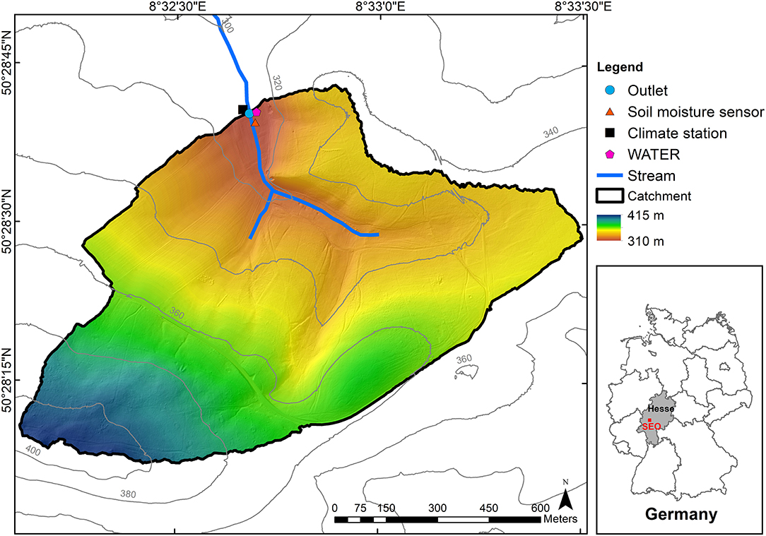
Figure 1. Location of the Schwingbach Environmental Observatory (SEO) in Hesse, Germany (red square, right panel) and a map of the study area in the headwater catchment of the SEO including the measuring network.

Precipitation depth and air temperature were recorded at 5 min intervals with an automated climate station (AQ5, Campbell Scientific Inc., Shepshed, UK) operated with a CR1000 data logger. Soil moisture was measured at 5, 30, and 70 cm depths at the toeslope at 5 min intervals with a remote telemetry logger (A753, Adcon, Klosterneuburg, Austria) equipped with capacitance sensors (ECH2O 5TE, METER Environment, Pullman, USA). Stream water at the outlet of the catchment and precipitation were automatically sampled for stable isotopes of water in situ using an automated mobile laboratory, the Water Analysis Trailer for Environmental Research (WATER), from August 8th until December 9th in 2018 and from April 12th until October 10th in 2019. If no precipitation occurred, stream water was sampled approximately every 90 min. Precipitation was automatically sampled if its depth exceeded 0.3 mm. It should be noticed that the SEO is not a snow-driven catchment. The precipitation events were all in form of rainfall with no snow included over the sampling period. After sampling, the precipitation sampler was blocked for 60 min. Isotopic composition of stream water and precipitation were measured using a continuous water sampler (CWS) (A0217, Picarro Inc., Santa Clara, USA), coupled to a wavelength-scanned cavity ring-down spectrometer (WS-CRDS) (L2130-i, Picarro Inc., Santa Clara, USA) inside the mobile laboratory. For detailed description of the WATER and the sampling procedures see Sahraei et al. (2020). The SEO was chosen in this study because of its responsive characteristic to precipitation inputs as well as the available extensive hydrological knowledge and data on the catchment (Lauer et al., 2013; Orlowski et al., 2014, 2016; Aubert et al., 2016; Sahraei et al., 2020). The runoff generation processes of the Schwingbach are characterized by a rapid mixing of streamflow with event water through shallow subsurface flow pathways. The high-resolution sampling of isotope concentrations and hydroclimatic data employed in this study allowed the detection of fine-scale, short-term responses, and mixing processes, which in turn provided the opportunity to capture a wide range of maximum event water fractions under different flow regimes and hydroclimatic conditions. The mean, standard deviation, Kurtosis and Skewness of the maximum event water fraction data are 32.4%, 24.2%, −0.4, and 0.8, respectively. These statistical values imply that the maximum event water fractions are highly dynamic in the SEO, which in turn provides the opportunity to test the capability and effectiveness of the ANN and SVM models for the prediction of maximum event water fractions at the event scale.

In this work, the precipitation events were defined as independent if the inter-event time exceeded 6 h, similar to the separation made by Sahraei et al. (2020). The dry period between two wet periods is known as the inter-event time, and if the dry period is equal to or longer than the desired inter-event time, the two wet periods are considered as two independent events (Balistrocchi and Bacchi, 2011; Chin et al., 2016). In total, 40 events were selected over the sampling period (Figure 2), for which the application of isotopic hydrograph separation was possible. The isotopic hydrograph separation was not possible for other events because either the isotopic compositions of stream water and precipitation were not available or because the difference between the isotopic composition of stream water and precipitation was too small. For the selected events, the beginning of the event was defined as the onset of precipitation and the end of the event as the time when either the event water fraction declined to 5% of its peak value or another precipitation event began, whichever first occurred.

FIGURE 2

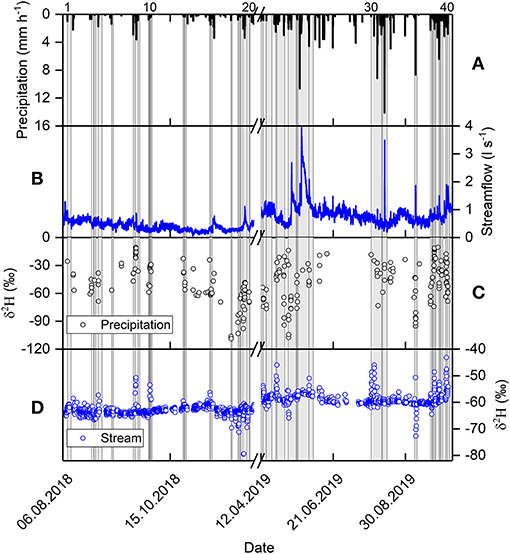
Figure 2. Time series of (A) precipitation, (B) streamflow, (C) δ²H in precipitation and (D) δ²H in streamflow. The vertical gray bars indicate the 40 events. The numbers on top of panel (A) represent the event ID.

The event water fractions F_E was quantified for each event at ~90 min intervals using a two-component isotopic hydrograph separation according to Equation (1):

$\begin{array}{ll}{F}_E=\frac{C_S-C_P}{C_E-C_P}& (1)\end{array}$

where C_S, C_E, and C_P are the isotopic concentrations (δ²H) in the stream water, event water (i.e., precipitation) and pre-event water, respectively. C_S was measured at ~90 min intervals. C_E is the incremental weighted mean of precipitation samples (Mcdonnell et al., 1990), which were measured if the precipitation depth exceeded 0.3 mm. After sampling, the precipitation sampler was blocked for 60 min. C_P was calculated as the average of the last five samples, which were measured at ~90 min intervals before the onset of precipitation. The maximum event water fraction F_Emax, at which the event water contribution to streamflow reaches its peak value during the precipitation event, was obtained from maximum of F_E values over each of the 40 events. The F_Emax was the target variable predicted by the ANN and SVM models. Sahraei et al. (2020) reported that higher precipitation amounts generally lead to an increase of the maximum event water fraction in the streamflow as can be observed in Figure 3. This behavior is consistent with previous studies, which also reported growing maximum event water fractions with rising precipitation amounts (Pellerin et al., 2008; Penna et al., 2015; von Freyberg et al., 2017). This suggests that the Schwingbach is highly responsive to precipitation inputs and precipitation is a main driver of hydrological response behavior in the stream.

FIGURE 3

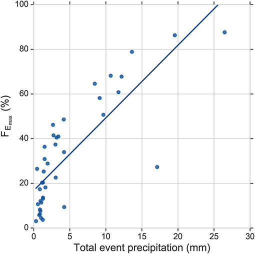
Figure 3. Maximum event water fraction F_Emax vs. total event precipitation.

The uncertainty of maximum event water fraction W_FEmax was quantified according to the Gaussian error propagation technique (Genereux, 1998):

$\begin{array}{l}{W}_{F_{E_{\max }}}=\{{\left[\frac{C_E-C_S}{{\left(C_E-C_P\right)}^2}{W}_{C_P}\right]}^2+{\left[\frac{C_S-C_P}{{\left(C_E-C_P\right)}^2}{W}_{C_E}\right]}^2\hfill \\ +{{\left[\frac{-1}{\left(C_E-C_P\right)}{W}_{C_S}\right]}^2\}}^{1/2}\hfill & (2)\end{array}$

W_CP, the uncertainty in pre-event water, was estimated using the standard deviation of the last five measurements before the onset of precipitation. W_CE, the uncertainty of the event water, is the standard deviation of the incremental weighted mean of precipitation. W_CS, the uncertainty of the stream water measurements, is the measurement precision of the CWS coupled to the WS-CRDS (0.57‰ for δ²H), which we derived from the standard deviation of the measurements during the last 3 min of the sampling period of stream water. The uncertainty of maximum event water fractions ranged from 1.2 to 28.3% with a mean of 6.7 ± 7.2% (mean ± standard deviation). The quantified uncertainty for maximum event water fractions of all 40 events are reported in Supplementary Table 1.

As the inputs for the models, a set of hydroclimatic variables representing the precipitation and antecedent wetness characteristics of the Schwingbach catchment was selected. Total event precipitation (P, mm), precipitation duration (D, h), 3-day antecedent precipitation defined as the accumulated precipitation over a 3-day window before the onset of a precipitation event (AP3, mm), 1 h averaged soil moisture before onset of precipitation at 5, 30, and 70 cm depths (SM, %), and mean daily air temperature (T, °C) were selected for each of the 40 events. The selection of input variables was based on the combination of a priori knowledge obtained from Sahraei et al. (2020) and expert knowledge. The values of input and output variables are presented in the Supplementary Table 1.

Machine Learning Algorithms

Artificial Neural Network (ANN) Theoretical Background

In this study, the Multilayer Perceptron (MLP) feedforward neural network was applied, which is one of the most widely used ANNs in hydrology (Tanty and Desmukh, 2015; Oyebode and Stretch, 2018). The MLP network consists of a set of nodes organized into three different types of layers, i.e., input, hidden, and output layers (Figure 4). The input layer includes nodes, through which the input data is incorporated into the network. In the hidden layers, the nodes receive signals from the nodes in the previous layer via weighted connections, at which the weights determine the strength of the signals. The weighted values from the previous layer are summed together with a bias associated with the nodes. The result is then passed through an activation function to generate a signal (i.e., activation level) for each node. Next, the signals are transmitted to the subsequent layer and the process is continued until the information reaches the output layer. The signals, which are generated in the output layer are the model outputs. In general, the mathematical operation of a MLP feedforward neural network is given by Equation (3):

$\begin{array}{ll}{y}_j=f\left({\displaystyle \sum _{i=1}^n}\left(w_{ij}{x}_i\right)+b_j\right)& (3)\end{array}$

where x_i is the ith nodal value in the previous layer, y_j is the jth nodal value in the present layer, b_j is the bias of the jth node in the present layer, w_ij is a weight connecting x_i and y_j, n is the number of nodes in the previous layer, and f denotes the activation function in the present layer.

FIGURE 4

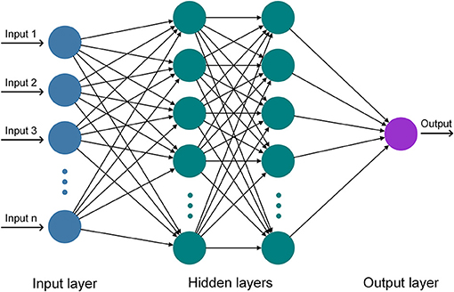
Figure 4. Schematic diagram of an Artificial Neural Network (ANN).

The backpropagation algorithm (Lecun et al., 2015) was used to train the network, in which the outputs produced in the output layer for the given inputs, are compared to the target values (i.e., observations) and the error is calculated through a loss function. If the output layer does not produce the desired values, the output errors are propagated backwards through the network, while the parameters of nodes (i.e., weights and bias) in each layer are updated along the way with an optimizer. The learning process repeats in this way for several rounds (i.e., epochs) until the loss function reaches an optimal value.

ANN Setup

The performance of the ANN model is strongly dependent on the configuration of its hyperparameters. Among the hyperparameters, the number of nodes in hidden layers, learning rate, and activation functions in hidden layers have the greatest influence on the model performance and its robustness (Smithson et al., 2016; Klein and Hutter, 2019). Therefore, a set of the aforementioned hyperparameters was defined to evaluate performance of 45 ANN model configurations resulting from discretizing the hyperparameters shown in Table 1. As the base architecture, an ANN model with seven nodes in the input layer, two hidden layers followed by a linear output layer with one node was defined. Previous studies have reported that networks with two hidden layers generally outperform those with a single hidden layer, since they are more stable, flexible, and also sufficient to approximate complex non-linear functions (Sontag, 1992; Flood and Kartam, 1994; Heaton, 2015; Thomas et al., 2017). The most challenging and time consuming aspect of neural network design is choosing the optimal number of hidden nodes (Thomas et al., 2016b). Too few hidden nodes implies that the network does not have enough capacity to solve the problem. Conversely, too many hidden nodes implies that the network memorizes noise within training data, leading to poor generalization capability (Maier and Dandy, 2000; Thomas et al., 2016b). The number of hidden nodes in the first and second hidden layers should be kept nearly equal to yield better generalization capability (Karsoliya, 2012). Given that, five different configurations shown in Table 1 were used for the number of hidden nodes according to Equations (4) and (5) expressed by Thomas et al. (2016a):

$\begin{array}{ll}{n}_h=n_1+n_2& (4)\end{array}$

$\begin{array}{ll}{n}_1=int\left(0.5n_h+1\right)& (5)\end{array}$

where n_h represents total number of hidden nodes, n₁ and n₂ represent number of nodes in the first and second hidden layer, respectively. The upper bound on the total number of hidden nodes was considered as half of the total number of samples (i.e., n_h = 20) suggested by previous studies (Tamura and Tateishi, 1997; Huang, 2003). The “Adam” optimizer was used for the optimization of the learning process, which is effective for dealing with non-linear problems, including outliers (Kingma and Ba, 2014). Learning rate is a positive number below 1 that scales the magnitude of the steps taken in the weight space in order to minimize the loss function of the network (Maier and Dandy, 2000; Heaton, 2015; Goodfellow et al., 2016). Too small learning rates slow down the learning process and may cause the learning to become stuck with a high learning error. On the other hand, too large learning rates can lead the network to go through large oscillations during the learning process or that the network may never converge (Maier and Dandy, 1998; Goodfellow et al., 2016). The default learning rate of the Adam optimizer is set to 0.001. The smaller (0.0001) and larger (0.01) learning rates were also tested. Sigmoid and hyperbolic tangent (Tanh) are the most common activation functions used in the feedforward networks (Maier and Dandy, 2000). However, Rectified Linear Unit (ReLU) is usually a more suitable choice (Heaton, 2015). Sigmoid, Tanh and ReLU as the activation functions of hidden layers were therefore tested. Each network was trained for a maximum of 10,000 epochs to minimize the mean absolute error (MAE).

TABLE 1

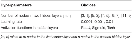
Table 1. Hyperparameter set for the ANN model.

Support Vector Machine (SVM) Theoretical Background

The Support Vector Machine (SVM) was first proposed by Cortes and Vapnik (1995). It is based on statistical learning theory and is derived from the structural risk minimization hypothesis to minimize both empirical risk and the confidence interval of the learning machine in order to achieve good generalization capability. In this study, the Support Vector Regression (SVR) was used, which is an adaptation of the SVM algorithm for regression problems (Vapnik et al., 1997; Smola and Schölkopf, 2004). The basic concept of the SVR is to non-linearly map the original data in a higher dimensional feature space and to solve a linear regression problem in the feature space (Figure 5). Suppose a series of data points ${\left\{x_i,y_i\right\}}_i^n$, where n is the data size, x_i is the input vector and y_i represents the target value, the SVR function is as follows:

$\begin{array}{ll}f\left(x_i\right)=w·\varphi \left(x_i\right)+b& (6)\end{array}$

where w is a weight vector and b is a bias. ϕ(x_i) denotes a non-linear mapping function that maps the inputs vectors to a high-dimensional feature space. w and b are estimated by minimizing the regularized risk function, as shown in Equation (7):

$\begin{array}{ll}R\left(w\right)=\frac{1}{2}{\Vert w\Vert }^2+C{\displaystyle \sum _{i=1}^n}{L}_{\epsilon }\left(y_i,f\left(x_i\right)\right)& (7)\end{array}$

where 1/2||w||² is a regularization term, C is the penalty coefficient, which is considered to specify the trade-off between the empirical risk and the model flatness and L_ε(y_i, f(x_i)) is called the ε-insensitive loss function, which is defined according to Equation (8):

$\begin{array}{ll}{L}_{\epsilon }\left(y_i,f\left(x_i\right)\right)=max\left\{0,|y_i-f\left(x_i\right)|-\epsilon \right\}& (8)\end{array}$

where ε denotes the permitted error threshold. ε will be ignored if the predicted value is within the threshold; otherwise, the loss equals a value greater than ε. In order to represent the distance from actual values to the corresponding boundary values of the ε-tube, two positive slack variables ξ and ξ^* are introduced. Then Equation (7) is transformed into the following constrained form:

$\begin{array}{ll}minf\left(w,\xi ,{\xi }^{*}\right)=\frac{1}{2}{\Vert w\Vert }^2+C{\displaystyle \sum _{i=1}^n}\left(\xi +{\xi }^{*}\right)& (9)\end{array}$

Subject to:

$\begin{array}{ll}\{\begin{array}{c}{y}_i-\left[w·\varphi \left(x_i\right)\right]-b\le \epsilon +\xi ,\xi \ge 0\\ \left[w·\varphi \left(x_i\right)\right]+b-y_i\le \epsilon +{\xi }^{*},{\xi }^{*}\ge 0\end{array}& (10)\end{array}$

This constrained optimization problem can be solved by the following Lagrangian function:

$\begin{array}{l}maxH\left({\partial }_i,{\partial }_i^{*}\right)=-\frac{1}{2}{\displaystyle \sum _{i=1}^n}{\displaystyle \sum _{j=1}^n}\left({\partial }_i-{\partial }_i^{*}\right)\left({\partial }_j-{\partial }_j^{*}\right)K\left(x_i,x_j\right)\\ +{\displaystyle \sum _{i=1}^n}{y}_i\left({\partial }_i-{\partial }_i^{*}\right)-\epsilon {\displaystyle \sum _{i=1}^n}{y}_i\left({\partial }_i+{\partial }_i^{*}\right)& (11)\end{array}$

Subject to:

$\begin{array}{ll}{\displaystyle \sum _{i=1}^n}\left({\partial }_i-{\partial }_i^{*}\right)=0,{\partial }_i,{\partial }_i^{*}\in \left[0,C\right]& (12)\end{array}$

Therefore, the regression function is as follows:

$\begin{array}{ll}f\left(x\right)={\displaystyle \sum _{i=1}^n}\left({\partial }_i-{\partial }_i^{*}\right)K(x_i,x_j)+b& (13)\end{array}$

where K(x_i, x_j) is the kernel function and ∂_i and ${\partial }_i^{*}$ are the non-negative Lagrangian multipliers, respectively. The kernel function can non-linearly map the original data into a higher dimensional feature space in an implicit manner and solve a linear regression problem in the feature space.

FIGURE 5

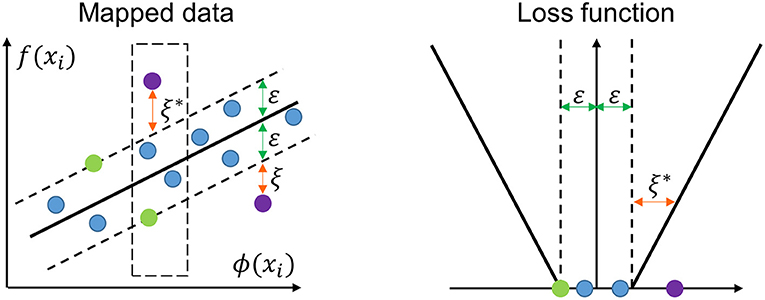
Figure 5. Schematic diagram of a Support Vector Regression (SVR).

SVM Setup

The performance of the SVM model is directly related to the selection of the kernel function (Raghavendra and Deka, 2014; Zhang et al., 2018). In this study, the performances of four commonly employed kernels in SVM studies including the Linear, Sigmoid, Radial Basis Function (RBF), and Polynomial kernels combined with their optimal hyperparameters were tested. The Linear kernel has two hyperparameters (C, ε), the Sigmoid and RBF kernels have three hyperparameters (C, ε, γ), and the Polynomial kernel has four hyperparameters (C, ε, γ, d) to be optimized. The penalty coefficient C, determines the tolerance of deviations larger than ε from the real value; i.e., smaller deviations are tolerable for larger values of C. The permitted error threshold ε, affects the number of support vectors used in the regression function, i.e., the smaller the value of ε, the greater the number of support vectors that will be selected. The kernel coefficient γ, controls the influence radius of the support vectors, i.e., for high values of gamma, the radius of the influence area of the support vectors only includes the support vector itself. The degree of the polynomial function d, is the largest of the degrees of polynomial's monomials with non-zero coefficient. Twenty values for each of C, ε, and γ based on geometric progression and 3 values for d were tested according to the set of hyperparameters shown in Table 2. Therefore, 400 configurations for the Linear kernel, 8,000 configurations for the Sigmoid and RBF kernels and 24,000 configurations for the Polynomial kernel were tested. Finally, the performances between the kernel functions in combination with their optimal hyperparameter configurations were compared.

TABLE 2

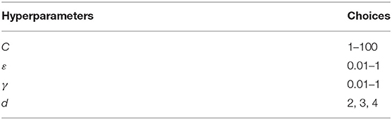
Table 2. Hyperparameter set for the kernel functions of the SVM model.

Model Evaluation

Repeated 10-fold cross-validation was performed to estimate the performance of the ANN and SVM models with different hyperparameter configurations. The data was first randomly shuffled and split into ten folds such that each fold contained four samples. For the ANN model, eight folds were considered for train set, one fold for validation set and one fold for test set. For the SVM model, nine fold were considered for train set and one fold for test set. The procedure was repeated 10 iterations so that in the end, every instance was used exactly once in the test set. Within each iteration of the cross-validation, the train set was normalized to be in the range [0-1]. To avoid data leakage, the test and validation sets were normalized using the parameters derived from train set normalization (Hastie et al., 2009). The train set was used to learn the internal parameters (i.e., weights and bias) of the network. The validation set was used for the hyperparameter optimization and the test set was used to estimate the generalization capability of the model (Goodfellow et al., 2016). The ANN model was first trained on the train set for 10,000 epochs to minimize the MAE on the validation set. The number of epochs, at which MAE of the validation set reached its minimum value, was saved. The validation set was then added to the train set and the whole data set was used to train the model for the fixed number of epochs derived from previous step. The test set was used to estimate the prediction performance of the ANN and SVM models. The estimation of model performance via one run of k-fold cross-validation might be noisy. This means that for each iteration of cross-validation, a different split of data set into k-folds can be implemented and in turn, the distribution of performance scores can be different, resulting in a different mean estimate of model performance (Brownlee, 2020). In order to reduce the noise and allow a reliable estimate of prediction performance, it is recommended to repeat the cross-validation procedure such that the data is re-shuffled before each round (Refaeilzadeh et al., 2009). The common numbers for repetition of cross-validation procedure are three, five, and ten (Kuhn and Johnson, 2013; Brownlee, 2020). To obtain a robust and reliable estimate for the model performance, the 10-fold cross-validation was repeated ten times with a different seed for the random shuffle generator, resulting in 100 iterations for each configuration. The performance of the ANN and SVM models were evaluated in terms of the MAE, the root mean squared error (RMSE), the coefficient of determination (R²), and Nash-Sutcliffe Efficiency (NSE) according to Equations (14), (15), (16), and (17), respectively. The optimized (i.e., best) configurations of the ANN and SVM were selected based on the average performance over 100 iterations. The performance of the optimized configuration of the ANN was then compared with that of the optimized configuration of the SVM to choose the final predictive model.

$\begin{array}{ll}MAE=\frac{1}{N}{\displaystyle \sum _{i=1}^N}|O_i-P_i|& (14)\end{array}$

$\begin{array}{ll}RMSE=\sqrt{\frac{1}{N}{\displaystyle \sum _{i=1}^N}{\left(O_i-P_i\right)}^2}& (15)\end{array}$

$\begin{array}{ll}{R}^2={\left[\frac{{\displaystyle {\sum }_{i=1}^N}\left(O_i-\overline{O}\right)\left(P_i-\overline{P}\right)}{\sqrt{{\displaystyle {\sum }_{i=1}^N}{\left(O_i-\overline{O}\right)}^2}\sqrt{{{\displaystyle {\sum }_{i=1}^N}\left(P_i-\overline{P}\right)}^2}}\right]}^2& (16)\end{array}$

$\begin{array}{ll}NSE=1-\frac{{\displaystyle {\sum }_{i=1}^N}{\left(O_i-P_i\right)}^2}{{\displaystyle {\sum }_{i=1}^N}{\left(O_i-\overline{O}\right)}^2}& (17)\end{array}$

where N is the number of observations (with N = 4 for the test set in each iteration of the cross-validation), O_i is the observed value, P_i is the predicted value, $\overline{O}$ is the mean of observed values, and $\overline{P}$ is the mean of predicted values. MAE and RMSE describe average deviation of predicted from observed values with smaller values indicating better performance. R² indicates correspondence between predicted and observed values with higher values [0 to 1] indicating stronger correlations. NSE evaluates the model ability to predict values different from the mean and gives the proportion of the initial variance accounted for by the model (Nash and Sutcliffe, 1970). NSE ranges between [–∞ to 1]. The closer the NSE value is to 1, the better is the agreement between predicted and observed values. A negative value of the NSE indicates that the mean of observed values is a better predictor than the proposed model. According to Moriasi et al. (2007), model performance can be evaluated as: very good (0.75 < NSE ≤ 1.00), good (0.65 < NSE ≤ 0.75), satisfactory (0.50 < NSE ≤ 0.65) and unsatisfactory (NSE ≤ 0.50).

Model Implementation

In this research, the numerical experiments were conducted with Python 3.7 programming environment (van Rossum, 1995) on Ubuntu 20.04 with AMD EPYC 7452 32-core processor, 125 GB of random access memory (RAM) and NVIDIA GTX 1050 Ti graphical processing unit (GPU). The ANN model was built with Keras 2.3.1 library (Chollet, 2015) on top of Theano backend 1.0.4 (Al-Rfou et al., 2016). The SVM model was built with Scikit-Learn 0.22.2 library (Pedregosa et al., 2011). Numpy 1.18.1 (Van Der Walt et al., 2011), Pandas 1.0.1 (McKinney, 2010), and Scipy 1.4.1 libraries (Virtanen et al., 2020) were used for preprocessing and data management. The Matplotlib 3.1.3 (Hunter, 2007) and Seaborn 0.9.1 (Waskom et al., 2020) libraries were used for the data visualization.

Results and Discussion

ANN Prediction Performance

The performance of 45 different ANN configurations were evaluated based on the number of nodes in hidden layers, learning rate, and activation functions in hidden layers. Table 3 shows the average prediction performance over 100 iterations of the cross-validation for each configuration in terms of MAE, RMSE, R², and NSE. The best performance was obtained by a combination of five nodes in the first hidden layer and three nodes in the second hidden layer [5, 3], a learning rate of 0.0001 and the Tanh activation function in hidden layers (configuration #12). This configuration resulted in a MAE of 10.27%, RMSE of 12.91%, R² of 0.70, and NSE of 0.63. Figure 6 shows the boxplots of statistical measures for prediction performance of 45 ANN configurations over 100 iterations of the cross-validation. The average is indicated by a black square and the median by the bar separating a box. It is clear from Figure 6 that configuration #1, #4, and #7 with three nodes in the first hidden layer and one node in the second hidden layer and ReLU activation function are the least stable networks, whereas the configuration #12 is the most stable network. Furthermore, it indicates that increasing the complexity of the network not only declines average model performance but also decreases the model stability as can be clearly seen on configurations #43 - #45. Table 3 shows that the performance of the 45 configurations based on the number of hidden nodes showed that increasing the number of nodes in hidden layers from eight [5, 3] to twenty [11, 9] did not have a major impact on the prediction performance and even the network with the highest number of hidden nodes [11, 9] did not yield the best prediction performance, whereas decreasing the number of hidden nodes to less than eight declined the model performance, particularly when the ReLU was used as the activation function. This implies that increasing the number of hidden nodes does not necessarily improve the ability of network to generalize, whereas decreasing the number of hidden nodes below a certain threshold may not be sufficient for the network to learn well. Similar behavior has been reported in the previous studies (Wilby et al., 2003; Yoon et al., 2011; Liu and Lu, 2014; Mohammadpour et al., 2015), emphasizing the importance of choosing an appropriate number of hidden nodes to ensure the model performance. Although the optimal number of hidden nodes depends on the essence and complexity of the problem (Maier and Dandy, 2000), the common challenge is to find an appropriate number of hidden nodes, which is sufficient to attain desired generalization capability in a reasonable training time (Maier and Dandy, 2000; Hagan et al., 2014; Goodfellow et al., 2016; Thomas et al., 2016b). The Adam optimizer is generally robust to the choice of its hyperparameters. However, the learning rate needs to be changed sometimes from the suggested default to improve the model performance (Kingma and Ba, 2014; Goodfellow et al., 2016). The smaller (0.0001) and larger (0.01) learning rates were therefore tested. In general, a change of the learning rate, while the number of hidden nodes and activation function were kept fixed, did not have a remarkable effect on the model performance. Nevertheless, the default learning rate still did not yield the best performance. An increase of the learning rate to 0.01 with fixed hidden nodes and activation function declined the performance, whereas the smaller learning rates (i.e., 0.0001 and 0.001) achieved slightly better performance. This implies that increasing the learning rate may cause the network to converge too quickly to a suboptimal solution, whereas smaller learning rate causes the network to take smaller steps toward minimum of the loss function leading to a better performance (Maier and Dandy, 1998). Smaller learning rates usually guarantee the convergence of the neural network; however, it is a trade-off between the model performance and the time required for the learning process (Heaton, 2015; Liu et al., 2019). It may be possible that our network achieves slightly better performance with the learning rates lower than 0.0001, but too long training time does not justify the use of smaller learning rates. It is almost impossible to make sure that the selected learning rate is the optimal learning rate, since any value falling between 0 and 1 can be considered for the learning rate (Najah Ahmed et al., 2019). However, it is suggested that testing the learning rate between 0.00001 and 0.1 by an order of magnitude usually ensures near-global optimal solution (Larochelle et al., 2007; Goodfellow et al., 2016; Géron, 2019). This range is usually shorter between 0.0001 and 0.01 when using the Adam optimizer (Poornima and Pushpalatha, 2019; Prasetya and Djamal, 2019; Feng et al., 2020). The Adam optimizer uses an adaptive learning rate algorithm leading the network to converge much faster compared to classical stochastic gradient descent (Kingma and Ba, 2014). Stochastic gradient descent maintains a single learning rate for all of its weight updates and the learning rate does not change during the learning process, whereas the Adam optimizer computes individual adaptive learning rates for different parameters from estimates of first and second moments of the gradients (Kingma and Ba, 2014). Among the activation functions, ReLU achieved the weakest performance with fixed hidden nodes and learning rate, whereas Sigmoid and Tanh activation functions yielded better, but nearly similar performances. The significant limitation of ReLU is that it easily overfits compared to the Sigmoid and Tanh activation functions (Nwankpa et al., 2018). ReLU is sometimes fragile during learning process causing some of the gradients to die. This leads to several nodes being dead as well, thereby causing the weight updates not to activate in future data points and hence, hindering a further learning as dead nodes give zero activation (Goodfellow et al., 2016; Nwankpa et al., 2018). Sigmoid and Tanh, both are monotonically increasing functions that asymptote a finite value as ±∞ is approached (LeCun et al., 2012). The only difference is that Sigmoid lies between 0 and 1, whereas Tanh lies between 1 and −1. One of the main advantages of Sigmoid and Tanh activation functions is that the activations (i.e., the values in the nodes of the network, not the gradients) may not explode during the learning process, since their output range is bounded (Feng and Lu, 2019; Szandała, 2020). However, it should be pointed out that each activation function has its own strengths and limitations and its performance may be different based on the network complexity and data structure (Nwankpa et al., 2018; Feng and Lu, 2019). Therefore, choosing a proper activation function should be prioritized to enhance the model performance. ANN model was trained for a maximum of 10,000 epochs to automatically optimize the number of epoch, at which the loss function (i.e., MAE) reaches its minimum on the validation set. Figure 7 shows MAE values over 10,000 training epochs on the normalized train and validation data over 100 iterations of the cross-validation for the optimized ANN model. The model converged within 6,000 epochs. The convergence behavior of the model indicates that the optimized model was robust and efficient in the learning process and that MAE was a proper loss function for the model to learn the problem.

TABLE 3

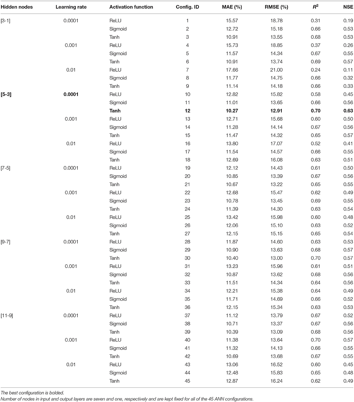
Table 3. Average prediction performance of the ANN model with different hyperparameter configurations over 100 iterations of the cross-validation.

FIGURE 6

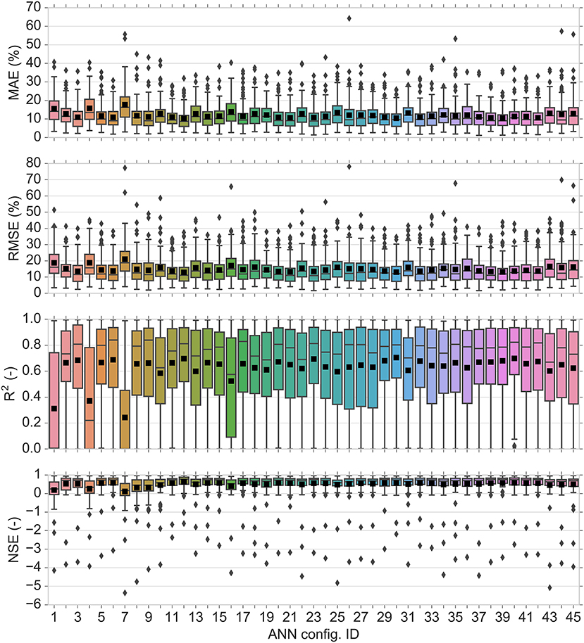
Figure 6. Boxplots of the performance criteria for prediction performance of 45 ANN configurations over 100 iterations derived from the ten times 10-fold cross-validation. The average is indicated by a black square and the median by the bar separating a box.

FIGURE 7

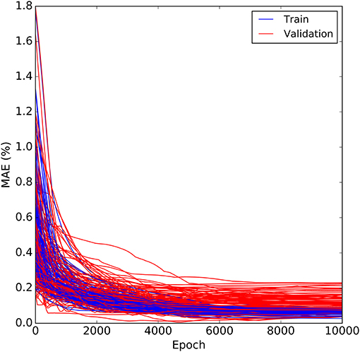
Figure 7. Loss function (MAE) vs. epoch on the normalized train and validation sets over 100 iterations derived from the ten times 10-fold cross-validation for the optimized ANN.

SVM Prediction Performance

The prediction performance of SVM was evaluated using various types of kernel functions in combination with the optimal hyperparameters of the kernel functions. Table 4 shows the average prediction performance over 100 iterations of the cross-validation for each kernel function with its optimal hyperparameters. The best prediction performance was obtained by a Polynomial kernel function with kernel hyperparameters of (C = 8.8587, ε = 0.0162, γ = 0.1833, d = 2). This configuration achieved a MAE of 7.89%, RMSE of 9.43%, R² of 0.83, and NSE of 0.78. The RBF kernel ranked second among the kernel functions. The Linear and Sigmoid kernels performed very similar to each other but slightly weaker than the RBF kernel. Figure 8 shows the boxplots of statistical measures for prediction performance of SVM kernels over 100 iterations of the cross-validation. It is observed that Linear and Sigmoid are the least stable kernels, whereas the Polynomial is the most stable kernel. The RBF kernel is more stable than Linear and Sigmoid kernels but less stable than Polynomial kernel. Our findings are in line with previous studies where Polynomial and RBF were found to be the most appropriate kernel functions that tend to give good performance for the modeling of the non-linear systems (Raghavendra and Deka, 2014). However, the RBF kernel is the mostly used kernel in previous studies (Raghavendra and Deka, 2014), since it has less hyperparameters than the Polynomial kernel that affect the complexity of model selection. Unlike the linear kernel, it can capture the non-linear relation between class labels and attributes and it tends to exhibit satisfactory performance under general smoothness assumptions (Raghavendra and Deka, 2014; Yaseen et al., 2015). The degree of polynomial function d defines the smoothness of the function, which gives the polynomial kernel the advantage of increasing the dimensionality (Raghavendra and Deka, 2014). For d = 2, the separation surfaces correspond to conic surfaces (i.e., an ellipse or hyperbola) in the feature space. Higher degrees can yield more complex decision boundaries, however, it may increase the risk of overfitting and hence, a decline in model performance (Yaman et al., 2012). Polynomial kernel takes the feature combinations implicitly into account instead of combining the features explicitly. By setting d, different numbers of feature conjunctions can be implicitly computed. In this way, Polynomial kernel performs often better than linear kernels, which do not utilize feature conjunctions (Wu et al., 2007).

TABLE 4

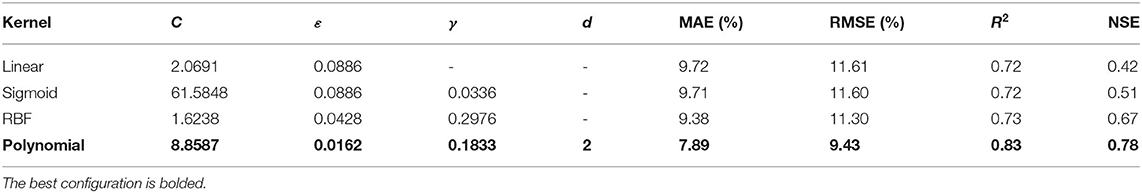
Table 4. Average prediction performance of the SVM model using different kernel functions with their optimal hyperparameters (C, ε, γ, d) over 100 iterations of the cross-validation.

FIGURE 8

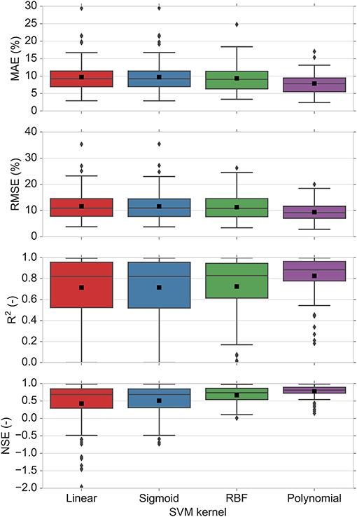
Figure 8. Boxplots of the performance criteria for prediction performance of SVM kernels over 100 iterations derived from the ten times 10-fold cross-validation. The average is indicated by a black square and the median by the bar separating a box.

Comparative Performance of Machine Learning Models

The optimized ANN and SVM models were selected based on the average performance over 100 iterations derived from ten times 10-fold cross-validation for an in-depth comparison of the models' capability in prediction of maximum event water fractions in the Schwingbach. Figure 9 shows the distribution of statistical measures for learning and prediction performance of the optimized ANN and SVM models over 100 iterations of the cross-validation. The optimized SVM outperformed the optimized ANN model in terms of performance and its stability. In terms of performance capability, the SVM achieved better performance in the train as well as in the test sets. The average and median values over the train and test sets were lower in terms of the MAE and RMSE, and higher in terms of the R² and NSE for the SVM compared to those of the ANN. In terms of performance stability, fewer variations were observed for the performance of the SVM model over the 100 iterations of cross-validation indicating that the SVM is a more stable model with respect to different train and test sets.

FIGURE 9

Figure 9. Boxplots of the performance criteria of the optimized ANN and optimized SVM for the train and test sets of 100 iterations derived from the ten times 10-fold cross-validation. The average is indicated by a black square and the median by the bar separating a box.

The 10-fold cross-validation strategy provides the opportunity for each data point to be predicted exactly once. Repeating this procedure ten times, results in ten predicted values for each data point, though over differently shuffled train and test sets. Figure 10 shows the comparison of observed and predicted maximum event water fractions of the 40 events by the optimized ANN and SVM models. The red and blue circles indicate the average of ten predicted values at each event by the optimized ANN and optimized SVM, respectively. The red and blue bands depict the range of all ten predicted values at each event by the optimized ANN and optimized SVM, respectively. Both models were able to reproduce the overall dynamic of maximum event water fractions across the events quite well. However, the optimized SVM model showed superiority over the optimized ANN model for predicting of the maximum event water fractions. Good match between observed and predicted maximum event water fractions was found using SVM model and generally, the predictions were closer to the corresponding observed values than those of the ANN model. The ANN tended to underestimate the events with high maximum event water fractions (e.g., events 4, 19, 32, and 37) and to overestimate the events with low maximum event water fractions (e.g., events 3, 6, 7, and 36). The main reason that the ANN may not be able to capture extreme values is the unavailability of the high number of extreme values in the training data, and hence the ANN cannot adequately learn the process in respect of extremes (Adnan et al., 2019a). The other main reason may be the fact that the ranges of extreme values in the training data are lower than those of the validation and/or test data (Adnan et al., 2019a; Malik et al., 2020). This leads to extrapolation difficulties in machine learning models (Kisi and Aytek, 2013; Kisi and Parmar, 2016). Several researchers have also reported this constraint in the application of the ANN in previous studies (Karunanithi et al., 1994; Minns and Hall, 1996; Dawson and Wilby, 1998; Campolo et al., 1999; Jimeno-Sáez et al., 2018; Singh et al., 2018; Najah Ahmed et al., 2019). It is evident that the range of all ten predicted values at each event was relatively high for the ANN model, particularly for the events with high maximum event water fractions. In contrast, this range was relatively low for the SVM model. It indicates that the performance of the SVM model for the prediction of maximum event water fraction is more reliable under randomly shuffled data compared to that of the ANN model.

FIGURE 10

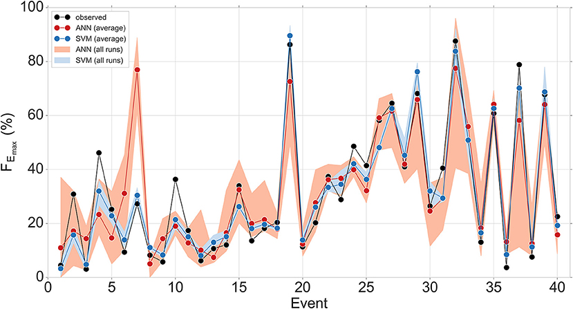
Figure 10. Comparison of observed and predicted maximum event water fractions F_Emax of the 40 events predicted by the optimized ANN and optimized SVM models. The red and blue circles indicate the average of ten predicted values at each event derived from ten times 10-fold cross-validation by the optimized ANN and SVM models, respectively. The red and blue bands indicate the range of all ten predicted values (i.e., all runs) at each event derived from ten times 10-fold cross-validation by the optimized ANN and SVM models, respectively.

The overall prediction ability of the SVM model was superior to that of the ANN model in this study. SVM implements the structural risk minimization principle, which gives it superior generalization ability in the situation of small sample size, whereas the ANN implements empirical risk minimization principle, which makes it more vulnerable to overfitting and susceptible to consider noise in the data as a pattern (Wu et al., 2008; Behzad et al., 2010; Yoon et al., 2011; Liu and Lu, 2014).

Application of Machine Learning on Small Data Set: Challenges and Strategies

Generally, the performance of machine learning models excels when having more training data available (Schmidhuber, 2015). Machine learning has exhibited promising performance in many fields such as natural language processing and image recognition where big data set is employed in training procedure (Feng et al., 2019). However, collecting training data set that is large enough is a challenge for some research fields such as medical, material, and natural sciences due to the complexity and high costs of data collection (Feng et al., 2019; Brigato and Iocchi, 2020). Compared to other areas of hydrological research, the available data is still limited in the field of isotope hydrology likely due to the laborious and cost intensive measurements of water isotopes. This lack of data is even more pronounced in case of high-resolution isotopic hydrographs at the event scale.

The key challenge on the application of machine learning on small data sets is that the model generalizes patterns in training data such that it correctly predicts unseen data on the test data set. The other main challenge is to ensure a reliable estimation for the generalization ability of the machine learning model. With the advance of machine learning during recent years, several strategies have been established to tackle data limitations that may affect the performance of the machine learning models. Resampling strategies like repeated k-fold cross-validation are the most appropriate for a small sample size (Kim, 2009; Refaeilzadeh et al., 2009; Beleites et al., 2013; Goodfellow et al., 2016). This strategy estimates the model performance by repeating the k-fold cross-validation procedure for number of times, where each time the data is shuffled randomly and subsequently the average performance over all iterations is reported. This is not only an unbiased estimate of model performance but also a reliable estimate of model performance and its stability with respect to different train and test sets (Kohavi, 1995; Beleites et al., 2013; Géron, 2019). Previous studies have successfully utilized cross-validation technique on small sample size ranging from 35 to 60 instances using SVM and ANN models (Behzad et al., 2010; Das et al., 2012; Khovanova et al., 2015; Shaikhina et al., 2015).

Model complexity is a critical factor when only limited data set is available. Using too complex models increases the likelihood of overfitting (Maier et al., 2010). Overfitting occurs when the model learns the details and noises in the training data to the extent that it fails to generalize on new data. On the other hand, using too simple models may lead to underfitting. Underfitting occurs when the model is too simple and does not have enough capacity to learn the patterns in the training data set. Ideally, it is desired to select a model at the sweet spot between underfitting and overfitting. In order to reduce the risk of underfitting and overfitting, a validation set was used to optimize the complexity of the models. Figure 6 shows that increasing the complexity of the ANN architecture does not enhance the performance of the model, whereas using too simple architectures does not lead to a promising performance too. This implies the importance and necessity of model complexity optimization in order to enhance the model performance especially in situation of small data set, for which the risk of underfitting and overfitting is even higher compared to larger data sets.

The choice of machine learning algorithm is another important factor that needs additional attention when dealing with limited data sets. SVM has shown to be a more suitable algorithm compared to ANN in the case of small sample sizes (Wu et al., 2008; Behzad et al., 2010; Das et al., 2012; Liu and Lu, 2014). Structural risk minimization and statistical machine learning process are the bases of SVM. The structural risk minimization aims to minimize the upper bound to the generalization error instead of traditional local training error. Moreover, SVM offers a unique and globally optimal solution towing to the convex characteristic of the ideal problem and employs high-dimensional spaced set of kernel functions that subtly includes non-linear transformation. Therefore, it has no hypothesis in functional transformation, which makes it essential to have linearly divisible data. At the same time, overfitting is unlikely to occur with the SVM, if the parameters are properly selected. Contrasting, ANN implements empirical risk minimization principle, which makes it more vulnerable to overfitting and falling into a local solution. The results showed that ANN was less stable compared to SVM (Figure 9). This might be due to the sensitivity of ANN to the initialization parameter values and training order (Bowden et al., 2002). ANN initialization and backpropagation training algorithms commonly contain deliberate degrees of randomness in order to improve convergence to the global optimal of the associated loss function (Wasserman, 1989; LeBaron and Weigend, 1998). Moreover, the order with which the training data is fed to the ANN may affect the level of convergence and produce erratic outcomes (LeBaron and Weigend, 1998). Such ANN volatilities limit the reproducibility of the results. The success of k-fold cross-validation to reduce the stability problems in ANNs has been discussed in previous studies (Maier and Dandy, 1998, 2000; Bowden et al., 2002). Nevertheless, additional care for optimization of hyperparameters and complexity of network needs to be taken when applying ANN to small sample size.

Conclusion

Estimating maximum event water fractions in streamflow based on the isotopic hydrograph separation gives valuable insight into runoff generation mechanisms and hydrological response characteristics of a catchment. However, such estimation is not always possible due to the spatiotemporal difficulties in sampling and measuring of stable isotopes of water. Therefore, there is a need for a proper predictive model to predict maximum event water fractions in streamflow even at times when no direct sampling and measurements of stable isotopes of water are available. As the relationships between the maximum event water fraction and its drivers are complex and non-linear, predictions using process-based models are difficult. Recently, machine learning algorithms have become increasingly popular in the field of hydrology due to their ability in representing complex and non-linear systems without any a priori assumption about the structure of the data and knowledge about the underlying physical processes. However, the potential of machine learning in the field of isotope hydrology has rarely been investigated. This study investigates the applicability of ANN and SVM algorithms to predict maximum event water fractions on independent events in the Schwingbach Environmental Observatory (SEO), Germany. The result showed that maximum event water fraction could be successfully predicted using only precipitation, soil moisture, and air temperature. This is very important in practice because sampling and measuring of stable isotopes of water are cost intensive, laborious, and often not feasible under difficult spatiotemporal conditions. It is concluded that SVM is superior to the ANN in the prediction of maximum event water fractions on independent precipitation events. SVM could better capture the dynamics of maximum event water fractions across the events and the predictions were generally closer to the corresponding observed values. ANN tended to underestimate the events with high maximum event water fractions and to overestimate the events with low maximum event water fractions. Detailed discussion is provided with respect to the influence of hyperparameters on the model performance.

Directions of future research include benchmarking the performance of the proposed machine learning models against process-based models in the field of isotope hydrology. Applying the proposed machine learning models with more training data and to other catchments in other parts of the world would allow assessing how well our method is transferable to catchments with different characteristics (e.g., weather patterns, topography, land use, and catchment size). Further, the proposed algorithms could be compared to other machine learning algorithms using different input scenarios of hydroclimatic data.

Using machine learning algorithms for the prediction of target variables that are difficult, expensive, or cumbersome to measure provides a valuable tool for future applications. Such algorithms can also be of great value for gap filling procedures. Our study focuses on machine learning in the field of isotope hydrology, but further applications in hydro-chemistry, e.g., for the prediction of pesticides or antibiotics have great potential for future research.

Machine learning does not substitute monitoring efforts as the model development is based on the robust data that covers diverse flow situations. However, machine learning is seen as a promising supplement for the establishment of long-term monitoring strategies of hydrological systems.

Data Availability Statement

The datasets presented in this study can be found in online repositories. The names of the repository/repositories and accession number(s) can be found at: The Zenodo repository, http://doi.org/10.5281/zenodo.4275329.

Author Contributions

AS, AC, and LB conceptualized the research. AS performed data acquisition, data analysis, and model development. PK established the requirements for the use of the graphic processing unit. AS prepared the manuscript with contribution from all authors. LB, AC, and PK reviewed and revised the manuscript. LB supervised the project. All authors have read and approved the content of the manuscript.

Conflict of Interest

The authors declare that the research was conducted in the absence of any commercial or financial relationships that could be construed as a potential conflict of interest.

Supplementary Material

The Supplementary Material for this article can be found online at: https://www.frontiersin.org/articles/10.3389/frwa.2021.652100/full#supplementary-material

References

Abdollahi, S., Raeisi, J., Khalilianpour, M., Ahmadi, F., and Kisi, O. (2017). Daily mean streamflow prediction in perennial and non-perennial rivers using four data driven techniques. Water Resour. Manage. 31, 4855–4874. doi: 10.1007/s11269-017-1782-7

CrossRef Full Text | Google Scholar

Adeyemi, O., Grove, I., Peets, S., Domun, Y., and Norton, T. (2018). Dynamic neural network modelling of soil moisture content for predictive irrigation scheduling. Sensors 18:3408. doi: 10.3390/s18103408

PubMed Abstract | CrossRef Full Text | Google Scholar

Adnan, R. M., Khosravinia, P., Karimi, B., and Kisi, O. (2021a). Prediction of hydraulics performance in drain envelopes using Kmeans based multivariate adaptive regression spline. Appl. Soft Comput. 100:107008. doi: 10.1016/j.asoc.2020.107008

CrossRef Full Text | Google Scholar

Adnan, R. M., Liang, Z., Heddam, S., Zounemat-Kermani, M., Kisi, O., and Li, B. (2019a). Least square support vector machine and multivariate adaptive regression splines for streamflow prediction in mountainous basin using hydro-meteorological data as inputs. J. Hydrol. 586:124371. doi: 10.1016/j.jhydrol.2019.124371

CrossRef Full Text | Google Scholar

Adnan, R. M., Liang, Z., Parmar, K. S., Soni, K., and Kisi, O. (2021b). Modeling monthly streamflow in mountainous basin by MARS, GMDH-NN and DENFIS using hydroclimatic data. Neural Comput. Appl. 33, 2853–2871. doi: 10.1007/s00521-020-05164-3

CrossRef Full Text | Google Scholar

Adnan, R. M., Liang, Z., Trajkovic, S., Zounemat-Kermani, M., Li, B., and Kisi, O. (2019b). Daily streamflow prediction using optimally pruned extreme learning machine. J. Hydrol. 577:123981. doi: 10.1016/j.jhydrol.2019.123981

CrossRef Full Text | Google Scholar

Agyare, W. A., Park, S. J., and Vlek, P. L. G. (2007). Artificial neural network estimation of saturated hydraulic conductivity. Vadose Zoo. J. 6, 423–431. doi: 10.2136/vzj2006.0131

CrossRef Full Text | Google Scholar

Ahmad, S., Kalra, A., and Stephen, H. (2010). Estimating soil moisture using remote sensing data: a machine learning approach. Adv. Water Resour. 33, 69–80. doi: 10.1016/j.advwatres.2009.10.008

CrossRef Full Text | Google Scholar

Al-Rfou, R., Alain, G., Almahairi, A., Angermueller, C., Bahdanau, D., Ballas, N., et al. (2016). Theano: a Python framework for fast computation of mathematical expressions. arXiv Preprint arXiv1605.02688v1.

Google Scholar

Araya, S. N., and Ghezzehei, T. A. (2019). Using machine learning for prediction of saturated hydraulic conductivity and its sensitivity to soil structural perturbations. Water Resour. Res. 55, 5715–5737. doi: 10.1029/2018WR024357

CrossRef Full Text | Google Scholar

ASCE Task Committee on Application of Artificial Neural Networks in Hydrology (2000). Artificial neural networks in hydrology. I: preliminary concepts. J. Hydrol. Eng. 5, 115–123. doi: 10.1061/(ASCE)1084-0699(2000)5:2(115)

CrossRef Full Text | Google Scholar

Aubert, A. H., Thrun, M. C., Breuer, L., and Ultsch, A. (2016). Knowledge discovery from high-frequency stream nitrate concentrations: hydrology and biology contributions. Sci. Rep. 6:31536. doi: 10.1038/srep31536

PubMed Abstract | CrossRef Full Text | Google Scholar

Balistrocchi, M., and Bacchi, B. (2011). Modelling the statistical dependence of rainfall event variables through copula functions. Hydrol. Earth Syst. Sci. 15, 1959–1977. doi: 10.5194/hess-15-1959-2011

CrossRef Full Text | Google Scholar

Behzad, M., Asghari, K., and Coppola, E. A. (2010). Comparative study of SVMs and ANNs in aquifer water level prediction. J. Comput. Civ. Eng. 24, 408–413. doi: 10.1061/(ASCE)CP.1943-5487.0000043

CrossRef Full Text | Google Scholar

Beleites, C., Neugebauer, U., Bocklitz, T., Krafft, C., and Popp, J. (2013). Sample size planning for classification models. Anal. Chim. Acta 760, 25–33. doi: 10.1016/j.aca.2012.11.007

PubMed Abstract | CrossRef Full Text | Google Scholar

Benardos, P. G., and Vosniakos, G. C. (2007). Optimizing feedforward artificial neural network architecture. Eng. Appl. Artif. Intell. 20, 365–382. doi: 10.1016/j.engappai.2006.06.005

CrossRef Full Text | Google Scholar

Bowden, G. J., Maier, H. R., and Dandy, G. C. (2002). Optimal division of data for neural network models in water resources applications. Water Resour. Res. 38, 2-1–2-11. doi: 10.1029/2001wr000266

CrossRef Full Text | Google Scholar

Brielmann, H. (2008). Recharge and Discharge Mechanism and Dynamics in the Mountainous Northern Upper Jordan River Catchment, Israel. Available online at: https://edoc.ub.uni-muenchen.de/9972/1/Brielmann_Heike.pdf

Google Scholar

Brigato, L., and Iocchi, L. (2020). A Close Look at deep learning with small data. arXiv Preprint arXiv2003.12843.

Google Scholar

Brown, V. A., McDonnell, J. J., Burns, D. A., and Kendall, C. (1999). The role of event water, a rapid shallow flow component, and catchment size in summer stormflow. J. Hydrol. 217, 171–190. doi: 10.1016/S0022-1694(98)00247-9

CrossRef Full Text | Google Scholar

Brownlee, J. (2020). Repeated k-Fold Cross-Validation for Model Evaluation in Python. Available online at: https://machinelearningmastery.com/repeated-k-fold-cross-validation-with-python/ (accessed March 19, 2021).

Google Scholar

Buttle, J. M. (1994). Isotope hydrograph separations and rapid delivery of pre-event water from drainage basins. Prog. Phys. Geogr. 18, 16–41. doi: 10.1177/030913339401800102

CrossRef Full Text | Google Scholar

Campolo, M., Andreussi, P., and Soldati, A. (1999). River flood forecasting with a neural network model. Water Resour. Res. 35, 1191–1197. doi: 10.1029/1998WR900086

CrossRef Full Text | Google Scholar

Carey, S. K., and Quinton, W. L. (2005). Evaluating runoff generation during summer using hydrometric, stable isotope and hydrochemical methods in a discontinuous permafrost alpine catchment. Hydrol. Process. 19, 95–114. doi: 10.1002/hyp.5764

CrossRef Full Text | Google Scholar

Cerar, S., Mezga, K., Žibret, G., Urbanc, J., and Komac, M. (2018). Comparison of prediction methods for oxygen-18 isotope composition in shallow groundwater. Sci. Total Environ. 631–632, 358–368. doi: 10.1016/j.scitotenv.2018.03.033

PubMed Abstract | CrossRef Full Text | Google Scholar

Chen, D., Lu, J., and Shen, Y. (2010). Artificial neural network modelling of concentrations of nitrogen, phosphorus and dissolved oxygen in a non-point source polluted river in Zhejiang Province, southeast China. Hydrol. Process. 24, 290–299. doi: 10.1002/hyp.7482

CrossRef Full Text | Google Scholar

Chin, R. J., Lai, S. H., Chang, K. B., Jaafar, W. Z. W., and Othman, F. (2016). Relationship between minimum inter-event time and the number of rainfall events in Peninsular Malaysia. Weather 71, 213–218. doi: 10.1002/wea.2766

CrossRef Full Text | Google Scholar

Chollet, F. (2015). Keras. Available online at: https://keras.io

Google Scholar

Coopersmith, E. J., Minsker, B. S., Wenzel, C. E., and Gilmore, B. J. (2014). Machine learning assessments of soil drying for agricultural planning. Comput. Electron. Agric. 104, 93–104. doi: 10.1016/j.compag.2014.04.004

CrossRef Full Text | Google Scholar

Cortes, C., and Vapnik, V. (1995). Support-vector networks. Mach. Learn. 20, 273–297. doi: 10.1007/BF00994018

CrossRef Full Text | Google Scholar

Das, S. K., Samui, P., and Sabat, A. K. (2012). Prediction of field hydraulic conductivity of clay liners using an artificial neural network and support vector machine. Int. J. Geomech. 12, 606–611. doi: 10.1061/(asce)gm.1943-5622.0000129

CrossRef Full Text | Google Scholar

Dawson, C. W., and Wilby, R. (1998). An artificial neural network approach to rainfall-runoff modelling. Hydrol. Sci. J. 43, 47–66. doi: 10.1080/02626669809492102

CrossRef Full Text | Google Scholar

Dawson, C. W., and Wilby, R. L. (2001). Hydrological modelling using artificial neural networks. Prog. Phys. Geogr. 25, 80–108. doi: 10.1177/030913330102500104

CrossRef Full Text | Google Scholar

Duan, S., Ullrich, P., and Shu, L. (2020). Using convolutional neural networks for streamflow projection in California. Front. Water 2:28. doi: 10.3389/frwa.2020.00028

CrossRef Full Text | Google Scholar

Elbisy, M. S. (2015). Support Vector Machine and regression analysis to predict the field hydraulic conductivity of sandy soil. KSCE J. Civ. Eng. 19, 2307–2316. doi: 10.1007/s12205-015-0210-x

CrossRef Full Text | Google Scholar

Eshleman, K. N., Pollard, J. S., and O'Brien, A. K. (1993). Determination of contributing areas for saturation overland flow from chemical hydrograph separations. Water Resour. Res. 29, 3577–3587. doi: 10.1029/93WR01811

CrossRef Full Text | Google Scholar

Feng, J., and Lu, S. (2019). Performance analysis of various activation functions in artificial neural networks. J. Phys. Conf. Ser. 1237:022030. doi: 10.1088/1742-6596/1237/2/022030

CrossRef Full Text | Google Scholar

Feng, S., Zhou, H., and Dong, H. (2019). Using deep neural network with small dataset to predict material defects. Mater. Des. 162, 300–310. doi: 10.1016/j.matdes.2018.11.060

CrossRef Full Text | Google Scholar

Feng, X., Ma, G., Su, S. F., Huang, C., Boswell, M. K., and Xue, P. (2020). A multi-layer perceptron approach for accelerated wave forecasting in Lake Michigan. Ocean Eng. 211:107526. doi: 10.1016/j.oceaneng.2020.107526

CrossRef Full Text | Google Scholar

Fischer, B. M. C., Stähli, M., and Seibert, J. (2017a). Pre-event water contributions to runoff events of different magnitude in pre-alpine headwaters. Hydrol. Res. 48, 28–47. doi: 10.2166/nh.2016.176

CrossRef Full Text | Google Scholar

Fischer, B. M. C., van Meerveld, H. J., and Seibert, J. (2017b). Spatial variability in the isotopic composition of rainfall in a small headwater catchment and its effect on hydrograph separation. J. Hydrol. 547, 755–769. doi: 10.1016/j.jhydrol.2017.01.045

CrossRef Full Text | Google Scholar

Flood, I., and Kartam, N. (1994). Neural networks in civil engineering. I: principles and understanding. J. Comput. Civ. Eng. 8, 131–148. doi: 10.1061/(ASCE)0887-3801(1994)8:2(131)

CrossRef Full Text | Google Scholar

Genereux, D. (1998). Quantifying uncertainty in tracer-based hydrograph separations. Water Resour. Res. 34, 915–919. doi: 10.1029/98WR00010

CrossRef Full Text | Google Scholar

Genereux, D. P., and Hooper, R. P. (1998). “Oxygen and hydrogen isotopes in rainfall-runoff studies,” in Isotope Tracers in Catchment Hydrology, eds C. Kendall and J. J. McDonnell (Amsterdam: Elsevier), 319–346.

Google Scholar

Géron, A. (2019). Hands-On Machine Learning With Scikit-Learn, Keras, and TensorFlow: Concepts, Tools, and Techniques to Build Intelligent Systems. Sebastopol, CA: O'Reilly Media.

Google Scholar

Gill, M. K., Asefa, T., Kemblowski, M. W., and McKee, M. (2006). Soil moisture prediction using support vector machines. J. Am. Water Resour. Assoc. 42, 1033–1046. doi: 10.1111/j.1752-1688.2006.tb04512.x

CrossRef Full Text | Google Scholar

Goodfellow, I., Bengio, Y., and Courville, A. (2016). Deep Learning. Cambridge: MIT Press.

Google Scholar

Granata, F., Papirio, S., Esposito, G., Gargano, R., and de Marinis, G. (2017). Machine learning algorithms for the forecasting of wastewater quality indicators. Water 9:105. doi: 10.3390/w9020105

CrossRef Full Text | Google Scholar

Hagan, M. T., Demuth, H. B., and Beale, M. H. (2014). Neural Network Design. Stillwater, OK: Martin Hagan.

Google Scholar

Han, D., Chan, L., and Zhu, N. (2007). Flood forecasting using support vector machines. J. Hydroinformatics 9, 267–276. doi: 10.2166/hydro.2007.027

CrossRef Full Text | Google Scholar

Hastie, T., Tibshirani, R., and Friedman, J. (2009). The Elements of Statistical Learning: Data Mining, Inference, and Prediction. New York, NY: Springer Science and Business Media.

Google Scholar

Haykin, S. (1994). Neural Networks: A Comprehensive Foundation. Hoboken, NY: Prentice Hall PTR.

He, Z., Wen, X., Liu, H., and Du, J. (2014). A comparative study of artificial neural network, adaptive neuro fuzzy inference system and support vector machine for forecasting river flow in the semiarid mountain region. J. Hydrol. 509, 379–386. doi: 10.1016/j.jhydrol.2013.11.054

CrossRef Full Text | Google Scholar

Heaton, J. (2015). Artificial Intelligence for Humans, Volume 3: Deep Learning and Neural Networks. Chesterfield, MO: Heaton Research, Inc.

Google Scholar

Hoeg, S., Uhlenbrook, S., and Leibundgut, C. (2000). Hydrograph separation in a mountainous catchment — combining hydrochemical and isotopic tracers. Hydrol. Process. 14, 1199–1216. doi: 10.1002/(SICI)1099-1085(200005)14:7<1199::AID-HYP35>3.0.CO;2-K

CrossRef Full Text | Google Scholar

Huang, G., Bin (2003). Learning capability and storage capacity of two-hidden-layer feedforward networks. IEEE Trans. Neural Netw. 14, 274–281. doi: 10.1109/TNN.2003.809401

PubMed Abstract | CrossRef Full Text | Google Scholar

Hunter, J. D. (2007). Matplotlib: a 2D graphics environment. IEEE Ann. Hist. Comput. 9, 90–95. doi: 10.1109/MCSE.2007.55

CrossRef Full Text | Google Scholar

Jain, S. K. (2012). Modeling river stage-discharge-sediment rating relation using support vector regression. Hydrol. Res. 43, 851–861. doi: 10.2166/nh.2011.101

CrossRef Full Text | Google Scholar

Jimeno-Sáez, P., Senent-Aparicio, J., Pérez-Sánchez, J., and Pulido-Velazquez, D. (2018). A comparison of SWAT and ANN models for daily runoff simulation in different climatic zones of Peninsular Spain. Water 10:192. doi: 10.3390/w10020192

CrossRef Full Text | Google Scholar

Kardan Moghaddam, H., Ghordoyee Milan, S., Kayhomayoon, Z., Rahimzadeh kivi, Z., and Arya Azar, N. (2021). The prediction of aquifer groundwater level based on spatial clustering approach using machine learning. Environ. Monit. Assess. 193:173. doi: 10.1007/s10661-021-08961-y

PubMed Abstract | CrossRef Full Text | Google Scholar

Karsoliya, S. (2012). Approximating number of hidden layer neurons in multiple hidden layer BPNN architecture. Int. J. Eng. Trends Technol. 3, 714–717.

Google Scholar

Karunanithi, N., Grenney, W. J., Whitley, D., and Bovee, K. (1994). Neural networks for river flow prediction. J. Comput. Civ. Eng. 8, 201–220. doi: 10.1061/(ASCE)0887-3801(1994)8:2(201)

CrossRef Full Text | Google Scholar

Khashei, M., and Bijari, M. (2010). An artificial neural network (p, d, q) model for timeseries forecasting. Expert Syst. Appl. 37, 479–489. doi: 10.1016/j.eswa.2009.05.044

CrossRef Full Text | Google Scholar

Khovanova, N. A., Shaikhina, T., and Mallick, K. K. (2015). Neural networks for analysis of trabecular bone in osteoarthritis. Bioinspir. Biomim. Nanobiomater. 4, 90–100. doi: 10.1680/bbn.14.00006

CrossRef Full Text | Google Scholar

Kim, J. H. (2009). Estimating classification error rate: repeated cross-validation, repeated hold-out and bootstrap. Comput. Stat. Data Anal. 53, 3735–3745. doi: 10.1016/j.csda.2009.04.009

CrossRef Full Text | Google Scholar

Kingma, D. P., and Ba, J. L. (2014). Adam: a method for stochastic optimization. arXiv Preprint arXiv1412.6980.

Google Scholar

Kisi, O., and Aytek, A. (2013). Explicit neural network in suspended sediment load estimation. Neural Netw. World 23, 587–607. doi: 10.14311/NNW.2013.23.035

CrossRef Full Text | Google Scholar

Kisi, O., and Parmar, K. S. (2016). Application of least square support vector machine and multivariate adaptive regression spline models in long term prediction of river water pollution. J. Hydrol. 534, 104–112. doi: 10.1016/j.jhydrol.2015.12.014

CrossRef Full Text | Google Scholar

Klaus, J., and McDonnell, J. J. (2013). Hydrograph separation using stable isotopes: review and evaluation. J. Hydrol. 505, 47–64. doi: 10.1016/j.jhydrol.2013.09.006

CrossRef Full Text | Google Scholar

Klein, A., and Hutter, F. (2019). Tabular benchmarks for joint architecture and hyperparameter optimization. arXiv Preprint arXiv1905.04970.

Google Scholar

Knoll, L., Breuer, L., and Bach, M. (2020). Nation-wide estimation of groundwater redox conditions and nitrate concentrations through machine learning. Environ. Res. Lett. 15:064004. doi: 10.1088/1748-9326/ab7d5c

CrossRef Full Text | Google Scholar

Kohavi, R. (1995). A Study of cross-validation and bootstrap for accuracy estimation and model selection. Int. Jt. Conf. Artif. Intell. 14, 1137–1145.

Google Scholar

Kong, Y., and Pang, Z. (2010). Isotope hydrograph separation in alpine catchments: a review. J. Glaciol. Geocryol. 32, 619–625. doi: 10.3724/SP.J.1226.2011.00086

CrossRef Full Text | Google Scholar

Kuhn, M., and Johnson, K. (2013). Applied Predictive Modeling. New York, NY: Springer. Available online at: http://appliedpredictivemodeling.com/s/Applied_Predictive_Modeling_in_R.pdf

Google Scholar

Kuppel, S., Tetzlaff, D., Maneta, M. P., and Soulsby, C. (2018). EcH2O-iso 1.0: water isotopes and age tracking in a process-based, distributed ecohydrological model. Geosci. Model Dev. 11, 3045–3069. doi: 10.5194/gmd-11-3045-2018

CrossRef Full Text | Google Scholar

Lange, H., and Sippel, S. (2020). “Machine learning applications in hydrology,” in Forest-Water Interactions, eds D. F. Levia, D. E. Carlyle-Moses, S. Iida, and B. Michalzik (Cham: Springer), 233–257.

Google Scholar

Larochelle, H., Erhan, D., Courville, A., Bergstra, J., and Bengio, Y. (2007). “An empirical evaluation of deep architectures on problems with many factors of variation,” in Proceedings of the 24th International Conference on Machine Learning (Corvallis, OR), 473–480.

Google Scholar

Lauer, F., Frede, H. G., and Breuer, L. (2013). Uncertainty assessment of quantifying spatially concentrated groundwater discharge to small streams by distributed temperature sensing. Water Resour. Res. 49, 400–407. doi: 10.1029/2012WR012537

CrossRef Full Text | Google Scholar

LeBaron, B., and Weigend, A. S. (1998). A bootstrap evaluation of the effect of data splitting on financial time series. IEEE Trans. Neural Netw. 9, 213–220. doi: 10.1109/72.655043

PubMed Abstract | CrossRef Full Text | Google Scholar

Lecun, Y., Bengio, Y., and Hinton, G. (2015). Deep learning. Nature 521, 436–444. doi: 10.1038/nature14539

CrossRef Full Text | Google Scholar

LeCun, Y., Bottou, L., Orr, G. B., and Müller, K. R. (2012). “Efficient Backpro,” in Neural Networks: Tricks of the Trade, eds G. Montavon, G. B. Orr, and K.-R. Müller (Berlin; Heidelberg: Springer), 9–48.

Google Scholar

Li, B., Yang, G., Wan, R., Dai, X., and Zhang, Y. (2016). Comparison of random forests and other statistical methods for the prediction of lake water level: A case study of the Poyang Lake in China. Hydrol. Res. 47, 69–83. doi: 10.2166/nh.2016.264

CrossRef Full Text | Google Scholar

Lin, J. Y., Cheng, C. T., and Chau, K. W. (2006). Using support vector machines for long-term discharge prediction. Hydrol. Sci. J. 51, 599–612. doi: 10.1623/hysj.51.4.599

CrossRef Full Text | Google Scholar

Lis, G., Wassenaar, L. I., and Hendry, M. J. (2008). High-precision laser spectroscopy D/H and 18O/16O measurements of microliter natural water samples. Anal. Chem. 80, 287–293. doi: 10.1021/ac701716q

PubMed Abstract | CrossRef Full Text | Google Scholar

Liu, M., and Lu, J. (2014). Support vector machine—an alternative to artificial neuron network for water quality forecasting in an agricultural nonpoint source polluted river? Environ. Sci. Pollut. Res. 21, 11036–11053. doi: 10.1007/s11356-014-3046-x

PubMed Abstract | CrossRef Full Text | Google Scholar

Liu, Y., Zhao, Q., Yao, W., Ma, X., Yao, Y., and Liu, L. (2019). Short-term rainfall forecast model based on the improved BP–NN algorithm. Sci. Rep. 9, 1–12. doi: 10.1038/s41598-019-56452-5

PubMed Abstract | CrossRef Full Text | Google Scholar

Maier, H. R., and Dandy, G. C. (1998). The effect of internal parameters and geometry on the performance of back-propagation neural networks: an empirical study. Environ. Model. Softw. 13, 193–209. doi: 10.1016/S1364-8152(98)00020-6

CrossRef Full Text | Google Scholar

Maier, H. R., and Dandy, G. C. (2000). Neural networks for the prediction and forecasting of water resources variables: a review of modelling issues and applications. Environ. Model. Softw. 15, 101–124. doi: 10.1016/S1364-8152(99)00007-9

CrossRef Full Text | Google Scholar

Maier, H. R., Jain, A., Dandy, G. C., and Sudheer, K. P. (2010). Methods used for the development of neural networks for the prediction of water resource variables in river systems: current status and future directions. Environ. Model. Softw. 25, 891–909. doi: 10.1016/j.envsoft.2010.02.003

CrossRef Full Text | Google Scholar

Malekzadeh, M., Kardar, S., and Shabanlou, S. (2019). Simulation of groundwater level using MODFLOW, extreme learning machine and Wavelet-Extreme Learning Machine models. Groundw. Sustain. Dev. 9:100279. doi: 10.1016/j.gsd.2019.100279

CrossRef Full Text | Google Scholar

Malik, A., Tikhamarine, Y., Souag-Gamane, D., Kisi, O., and Pham, Q. B. (2020). Support vector regression optimized by meta-heuristic algorithms for daily streamflow prediction. Stoch. Environ. Res. Risk Assess. 34, 1755–1773. doi: 10.1007/s00477-020-01874-1

CrossRef Full Text | Google Scholar

Matei, O., Rusu, T., Petrovan, A., and Mihut, G. (2017). A data mining system for real time soil moisture prediction. Procedia Eng. 181, 837–844. doi: 10.1016/j.proeng.2017.02.475

CrossRef Full Text | Google Scholar

Mcdonnell, J. J., Bonell, M., Stewart, M. K., and Pearce, A. J. (1990). Deuterium variations in storm rainfall: implications for stream hydrograph separation. Water Resour. Res. 26, 455–458. doi: 10.1029/WR026i003p00455

CrossRef Full Text | Google Scholar

McKinney, W. (2010). “Data structures for statistical computing in Python,” in Proceedings of the 9th Python in Science Conference (Austin, TX), 56–61.

Google Scholar

Minns, A. W., and Hall, M. J. (1996). Artificial neural networks as rainfall-runoff models. Hydrol. Sci. J. 41, 399–417. doi: 10.1080/02626669609491511

CrossRef Full Text | Google Scholar

Mohammadpour, R., Shaharuddin, S., Chang, C. K., Zakaria, N. A., Ghani, A. A., and Chan, N. W. (2015). Prediction of water quality index in constructed wetlands using support vector machine. Environ. Sci. Pollut. Res. 22, 6208–6219. doi: 10.1007/s11356-014-3806-7

PubMed Abstract | CrossRef Full Text | Google Scholar

Moriasi, D. N., Arnold, J. G., Van Liew, M. W., Bingner, R. L., Harmel, R. D., and Veith, T. L. (2007). Model evaluation guidelines for systematic quantification of accuracy in watershed simulations. Trans. Am. Soc. Agric. Biol. Eng. 50, 885–900. doi: 10.13031/2013.23153

CrossRef Full Text | Google Scholar

Najah Ahmed, A., Binti Othman, F., Abdulmohsin Afan, H., Khaleel Ibrahim, R., Ming Fai, C., Shabbir Hossain, M., et al. (2019). Machine learning methods for better water quality prediction. J. Hydrol. 578:124084. doi: 10.1016/j.jhydrol.2019.124084

PubMed Abstract | CrossRef Full Text | Google Scholar

Nash, J. E., and Sutcliffe, J. V. (1970). River flow forecasting through conceptual models part I—A discussion of principles. J. Hydrol. 10, 282–290. doi: 10.1016/0022-1694(70)90255-6

CrossRef Full Text | Google Scholar

Nwankpa, C., Ijomah, W., Gachagan, A., and Marshall, S. (2018). Activation functions: comparison of trends in practice and research for deep learning. arXiv Preprint arXiv1811.03378.

Google Scholar

Orlowski, N., Kraft, P., Pferdmenges, J., and Breuer, L. (2016). Exploring water cycle dynamics by sampling multiple stable water isotope pools in a developed landscape in Germany. Hydrol. Earth Syst. Sci. 20, 3873–3894. doi: 10.5194/hess-20-3873-2016

CrossRef Full Text | Google Scholar

Orlowski, N., Lauer, F., Kraft, P., Frede, H. G., and Breuer, L. (2014). Linking spatial patterns of groundwater table dynamics and streamflow generation processes in a small developed catchment. Water 6, 3085–3117. doi: 10.3390/w6103085

CrossRef Full Text | Google Scholar

Oyebode, O., and Stretch, D. S. (2018). Neural network modeling of hydrological systems: a review of implementation techniques. Nat. Resour. Model. 32:e12189. doi: 10.1002/nrm.12189

CrossRef Full Text | Google Scholar

Pedregosa, F., Varoquaux, G., Gramfort, A., Michel, V., Thirion, B., Grisel, O., et al. (2011). Scikit-learn: machine learning in Python. J. Mach. Learn. Res. 12, 2825–2830. doi: 10.5555/1953048.2078195

CrossRef Full Text | Google Scholar

Pellerin, B. A., Wollheim, W. M., Feng, X., and Vörösmarty, C. J. (2008). The application of electrical conductivity as a tracer for hydrograph separation in urban catchments. Hydrol. Process. 22, 1810–1818. doi: 10.1002/hyp.6786

CrossRef Full Text | Google Scholar

Penna, D., van Meerveld, H. J., Oliviero, O., Zuecco, G., Assendelft, R. S., Dalla Fontana, G., et al. (2015). Seasonal changes in runoff generation in a small forested mountain catchment. Hydrol. Process. 29, 2027–2042. doi: 10.1002/hyp.10347

CrossRef Full Text | Google Scholar

Penna, D., van Meerveld, H. J., Zuecco, G., Dalla Fontana, G., and Borga, M. (2016). Hydrological response of an Alpine catchment to rainfall and snowmelt events. J. Hydrol. 537, 382–397. doi: 10.1016/j.jhydrol.2016.03.040

CrossRef Full Text | Google Scholar

Piotrowski, A. P., Napiorkowski, M. J., Napiorkowski, J. J., and Osuch, M. (2015). Comparing various artificial neural network types for water temperature prediction in rivers. J. Hydrol. 529, 302–315. doi: 10.1016/j.jhydrol.2015.07.044

CrossRef Full Text | Google Scholar

Poornima, S., and Pushpalatha, M. (2019). Prediction of rainfall using intensified LSTM based recurrent neural network with weighted linear units. Atmosphere. 10:668. doi: 10.3390/atmos10110668

CrossRef Full Text | Google Scholar

Prasetya, E. P., and Djamal, E. C. (2019). “Rainfall forecasting for the natural disasters preparation using recurrent neural networks,” in International Conference on Electrical Engineering and Informatics (ICEEI) (Bandung), 52–57.

Google Scholar

Qiu, R., Wang, Y., Wang, D., Qiu, W., Wu, J., and Tao, Y. (2020). Water temperature forecasting based on modified artificial neural network methods: two cases of the Yangtze River. Sci. Total Environ. 737:139729. doi: 10.1016/j.scitotenv.2020.139729

PubMed Abstract | CrossRef Full Text | Google Scholar

Quan, Q., Hao, Z., Xifeng, H., and Jingchun, L. (2020). Research on water temperature prediction based on improved support vector regression. Neural Comput. Appl. 1–10. doi: 10.1007/s00521-020-04836-4

CrossRef Full Text | Google Scholar

Raghavendra, S., and Deka, P. C. (2014). Support vector machine applications in the field of hydrology: a review. Appl. Soft Comput. 19, 372–386. doi: 10.1016/j.asoc.2014.02.002

CrossRef Full Text | Google Scholar

Rasouli, K., Hsieh, W. W., and Cannon, A. J. (2012). Daily streamflow forecasting by machine learning methods with weather and climate inputs. J. Hydrol. 414–415, 284–293. doi: 10.1016/j.jhydrol.2011.10.039

CrossRef Full Text | Google Scholar

Refaeilzadeh, P., Lei, T., and Liu, H. (2009). “Cross-validation,” in Encyclopedia of Database Systems, eds L. Liu and M. T. Özsu (Boston, MA: Springer). doi: 10.1007/978-0-387-39940-9_565

CrossRef Full Text | Google Scholar

Renshaw, C. E., Feng, X., Sinclair, K. J., and Dums, R. H. (2003). The use of stream flow routing for direct channel precipitation with isotopically-based hydrograph separations: the role of new water in stormflow generation. J. Hydrol. 273, 205–216. doi: 10.1016/S0022-1694(02)00392-X

CrossRef Full Text | Google Scholar

Sahoo, S., Russo, T. A., Elliott, J., and Foster, I. (2017). Machine learning algorithms for modeling groundwater level changes in agricultural regions of the U.S. Water Resour. Res. 53, 3878–3895. doi: 10.1002/2016WR019933

CrossRef Full Text | Google Scholar

Sahraei, A., Kraft, P., Windhorst, D., and Breuer, L. (2020). High-resolution, in situ monitoring of stable isotopes of water revealed insight into hydrological behavior. Water 12:565. doi: 10.3390/w12020565

CrossRef Full Text | Google Scholar

Sahu, R. K., Müller, J., Park, J., Varadharajan, C., Arora, B., Faybishenko, B., et al. (2020). Impact of input feature selection on groundwater level prediction from a multi-layer perceptron neural network. Front. Water 2:573034. doi: 10.3389/frwa.2020.573034

CrossRef Full Text | Google Scholar

Sajedi-Hosseini, F., Malekian, A., Choubin, B., Rahmati, O., Cipullo, S., Coulon, F., et al. (2018). A novel machine learning-based approach for the risk assessment of nitrate groundwater contamination. Sci. Total Environ. 644, 954–962. doi: 10.1016/j.scitotenv.2018.07.054

PubMed Abstract | CrossRef Full Text | Google Scholar

Sattari, M. T., Mirabbasi, R., Sushab, R. S., and Abraham, J. (2018). Prediction of groundwater level in ardebil plain using support vector regression and M5 tree model. Groundwater 56, 636–646. doi: 10.1111/gwat.12620

PubMed Abstract | CrossRef Full Text | Google Scholar

Schmidhuber, J. (2015). Deep learning in neural networks: an overview. Neural Netw. 61, 85–117. doi: 10.1016/j.neunet.2014.09.003

PubMed Abstract | CrossRef Full Text | Google Scholar

Schölkopf, B., Smola, A. J., and Bach, F. (2002). Learning With Kernels: Support Vector Machines, Regularization, Optimization, and Beyond. Cambridge, MA: MIT Press.

Google Scholar

Senthil Kumar, A. R., Goyal, M. K., Ojha, C. S. P., Singh, R. D., and Swamee, P. K. (2013). Application of artificial neural network, fuzzylogic and decision tree algorithms for modelling of streamflow at Kasol in India. Water Sci. Technol. 68, 2521–2526. doi: 10.2166/wst.2013.491

PubMed Abstract | CrossRef Full Text | Google Scholar

Shahinfar, S., and Kahn, L. (2018). Machine learning approaches for early prediction of adult wool growth and quality in Australian Merino sheep. Comput. Electron. Agric. 148, 72–81. doi: 10.1016/j.compag.2018.03.001

CrossRef Full Text | Google Scholar

Shaikhina, T., Lowe, D., Daga, S., Briggs, D., Higgins, R., and Khovanova, N. (2015). Machine learning for predictive modelling based on small data in biomedical engineering. IFAC PapersOnLine 48, 469–474. doi: 10.1016/j.ifacol.2015.10.185

CrossRef Full Text | Google Scholar

Shortridge, J. E., Guikema, S. D., and Zaitchik, B. F. (2016). Machine learning methods for empirical streamflow simulation: a comparison of model accuracy, interpretability, and uncertainty in seasonal watersheds. Hydrol. Earth Syst. Sci. 20, 2611–2628. doi: 10.5194/hess-20-2611-2016

CrossRef Full Text | Google Scholar

Sihag, P. (2018). Prediction of unsaturated hydraulic conductivity using fuzzy logic and artificial neural network. Model. Earth Syst. Environ. 4, 189–198. doi: 10.1007/s40808-018-0434-0

CrossRef Full Text | Google Scholar

Singh, A., Malik, A., Kumar, A., and Kisi, O. (2018). Rainfall-runoff modeling in hilly watershed using heuristic approaches with gamma test. Arab. J. Geosci. 11:261. doi: 10.1007/s12517-018-3614-3

CrossRef Full Text | Google Scholar

Singh, K. P., Basant, N., and Gupta, S. (2011). Support vector machines in water quality management. Anal. Chim. Acta 703, 152–162. doi: 10.1016/j.aca.2011.07.027

PubMed Abstract | CrossRef Full Text | Google Scholar

Sklash, M. G., Farvolden, R. N., and Fritz, P. (1976). A conceptual model of watershed response to rainfall, developed through the use of oxygen-18 as a natural tracer. Can. J. Earth Sci. 13, 271–283. doi: 10.1139/e76-029

CrossRef Full Text | Google Scholar

Smithson, S. C., Yang, G., Gross, W. J., and Meyer, B. H. (2016). “Neural networks designing neural networks: multi-objective hyper-parameter optimization,” in Proceedings of the 35th International Conference on Computer-Aided Design (Austin, TX), 1–8.

Google Scholar

Smola, A. J., and Schölkopf, B. (2004). A tutorial on support vector regression. Stat. Comput. 14, 199–222. doi: 10.1023/B:STCO.0000035301.49549.88

CrossRef Full Text | Google Scholar

Sontag, E. D. (1992). Feedback stabilization using two-hidden-layer nets. IEEE Trans. Neural Netw. 3, 981–990. doi: 10.1109/72.165599

CrossRef Full Text | Google Scholar

Stadnyk, T. A., Delavau, C., Kouwen, N., and Edwards, T. W. D. (2013). Towards hydrological model calibration and validation: simulation of stable water isotopes using the isoWATFLOOD model. Hydrol. Process. 27, 3791–3810. doi: 10.1002/hyp.9695

CrossRef Full Text | Google Scholar

Szandała, T. (2020). “Review and comparison of commonly used activation functions for deep neural networks,” in Bio-inspired Neurocomputing (Singapore: Springer), 203–224.

Google Scholar

Tamura, S., and Tateishi, M. (1997). Capabilities of a four-layered feedforward neural network: four layers versus three. IEEE Trans. Neural Netw. 8, 251–255. doi: 10.1109/72.557662

PubMed Abstract | CrossRef Full Text | Google Scholar

Tanty, R., and Desmukh, T. S. (2015). Application of artificial neural network in hydrology- a review. Int. J. Eng. Res. Technol. 4, 184–188. doi: 10.17577/ijertv4is060247

CrossRef Full Text | Google Scholar

Tapoglou, E., Karatzas, G. P., Trichakis, I. C., and Varouchakis, E. A. (2014). A spatio-temporal hybrid neural network-Kriging model for groundwater level simulation. J. Hydrol. 519, 3193–3203. doi: 10.1016/j.jhydrol.2014.10.040

CrossRef Full Text | Google Scholar

Thomas, A. J., Petridis, M., Walters, S. D., Gheytassi, S. M., and Morgan, R. E. (2017). “Two hidden layers are usually better than one,” in International Conference on Engineering Applications of Neural Networks (Cham: Springer). doi: 10.1007/978-3-319-65172-9_24

CrossRef Full Text | Google Scholar

Thomas, A. J., Walters, S. D., Gheytassi, S. M., Morgan, R. E., and Petridis, M. (2016a). On the Optimal node ratio between hidden layers: a probabilistic study. Int. J. Mach. Learn. Comput. 6, 241–247. doi: 10.18178/ijmlc.2016.6.5.605

CrossRef Full Text | Google Scholar

Thomas, A. J., Walters, S. D., Petridis, M., Gheytassi, S. M., and Morgan, R. E. (2016b). “Accelerated optimal topology search for two-hidden- layer feedforward neural networks,” in International Conference on Engineering Applications of Neural Networks (Cham: Springer), 253–266. doi: 10.1007/978-3-319-44188-7_19

CrossRef Full Text | Google Scholar

Van Der Walt, S., Colbert, S. C., and Varoquaux, G. (2011). The NumPy array: a structure for efficient numerical computation. Comput. Sci. Eng. 13, 22–30. doi: 10.1109/MCSE.2011.37

CrossRef Full Text | Google Scholar

van Rossum, G. (1995). Python Tutorial. Amsterdam: Centrum voor Wiskunde en Informatica (CWI).

Google Scholar

Vapnik, V., Golowich, S. E., and Smola, A. (1997). “Support vector method for function approximation, regression estimation, and signal processing,” in Adv. Neural Inf. Process. Syst. (Cambridge, MA), 281–287.

Google Scholar

Virtanen, P., Gommers, R., Oliphant, T. E., Haberland, M., Reddy, T., Cournapeau, D., et al. (2020). SciPy 1.0: fundamental algorithms for scientific computing in Python. Nat. Methods 17, 261–272. doi: 10.1038/s41592-019-0686-2

PubMed Abstract | CrossRef Full Text | Google Scholar

von Freyberg, J., Studer, B., and Kirchner, J. W. (2017). A lab in the field: high-frequency analysis of water quality and stable isotopes in stream water and precipitation. Hydrol. Earth Syst. Sci. 21, 1721–1739. doi: 10.5194/hess-21-1721-2017

CrossRef Full Text | Google Scholar

Waskom, M., Botvinnik, O., Gelbart, M., Ostblom, J., Hobson, P., Lukauskas, S., et al. (2020). Seaborn: Statistical Data Visualization. Astrophys. Source Code Libr. ascl-2012.

Google Scholar

Wasserman, P. D. (1989). Neural Computing: Theory and Practice. New York, NY: Van Nostrand Reinhold Co.

Google Scholar

Wilby, R. L., Abrahart, R. J., and Dawson, C. W. (2003). Detection of conceptual model rainfall-runoff processes inside an artificial neural network. Hydrol. Sci. J. 48, 163–181. doi: 10.1623/hysj.48.2.163.44699

CrossRef Full Text | Google Scholar

Windhorst, D., Kraft, P., Timbe, E., Frede, H. G., and Breuer, L. (2014). Stable water isotope tracing through hydrological models for disentangling runoff generation processes at the hillslope scale. Hydrol. Earth Syst. Sci. 18, 4113–4127. doi: 10.5194/hess-18-4113-2014

CrossRef Full Text | Google Scholar

Wu, C. L., and Chau, K. W. (2010). Data-driven models for monthly streamflow time series prediction. Eng. Appl. Artif. Intell. 23, 1350–1367. doi: 10.1016/j.engappai.2010.04.003

CrossRef Full Text | Google Scholar

Wu, C. L., Chau, K. W., and Li, Y. S. (2008). River stage prediction based on a distributed support vector regression. J. Hydrol. 358, 96–111. doi: 10.1016/j.jhydrol.2008.05.028

CrossRef Full Text | Google Scholar

Wu, Y.-C., Yang, J.-C., and Lee, Y.-S. (2007). “An approximate approach for training polynomial kernel SVMs in linear time,” in Proceedings of the 45th Annual Meeting of the Association for Computational Linguistics Companion Volume Proceedings of the Demo and Poster Sessions (Prague), 65–68.

Google Scholar

Yaman, S., Pelecanos, J., and Omar, M. K. (2012). “On the use of nonlinear polynomial kernel SVMs in language recognition,” in 13th Annual Conference of the International Speech Communication Association (Portland, OR).

Google Scholar

Yang, T., Asanjan, A. A., Faridzad, M., Hayatbini, N., Gao, X., and Sorooshian, S. (2017). An enhanced artificial neural network with a shuffled complex evolutionary global optimization with principal component analysis. Inf. Sci. 418, 302–316. doi: 10.1016/j.ins.2017.08.003

CrossRef Full Text | Google Scholar

Yaseen, Z. M., El-shafie, A., Jaafar, O., Afan, H. A., and Sayl, K. N. (2015). Artificial intelligence based models for stream-flow forecasting: 2000-2015. J. Hydrol. 530, 829–844. doi: 10.1016/j.jhydrol.2015.10.038

CrossRef Full Text | Google Scholar

Yaseen, Z. M., Naghshara, S., Salih, S. Q., Kim, S., Malik, A., and Ghorbani, M. A. (2020). Lake water level modeling using newly developed hybrid data intelligence model. Theor. Appl. Climatol. 141, 1285–1300. doi: 10.1007/s00704-020-03263-8

CrossRef Full Text | Google Scholar

Yoon, H., Jun, S., Hyun, Y., Bae, G., and Lee, K. (2011). A comparative study of artificial neural networks and support vector machines for predicting groundwater levels in a coastal aquifer. J. Hydrol. 396, 128–138. doi: 10.1016/j.jhydrol.2010.11.002

CrossRef Full Text | Google Scholar

Yuan, X., Chen, C., Lei, X., Yuan, Y., and Adnan, R. M. (2018). Monthly runoff forecasting based on LSTM–ALO model. Stoch. Environ. Res. Risk Assess. 32, 2199–2212. doi: 10.1007/s00477-018-1560-y

CrossRef Full Text | Google Scholar

Zhang, D., Lin, J., Peng, Q., Wang, D., Yang, T., Sorooshian, S., et al. (2018). Modeling and simulating of reservoir operation using the artificial neural network, support vector regression, deep learning algorithm. J. Hydrol. 565, 720–736. doi: 10.1016/j.jhydrol.2018.08.050

CrossRef Full Text | Google Scholar

Zhang, Z., Chen, X., Cheng, Q., and Soulsby, C. (2019). Storage dynamics, hydrological connectivity and flux ages in a karst catchment: conceptual modelling using stable isotopes. Hydrol. Earth Syst. Sci. 23, 51–71. doi: 10.5194/hess-23-51-2019

CrossRef Full Text | Google Scholar

Zhu, S., Heddam, S., Wu, S., Dai, J., and Jia, B. (2019). Extreme learning machine-based prediction of daily water temperature for rivers. Environ. Earth Sci. 78, 1–17. doi: 10.1007/s12665-019-8202-7

CrossRef Full Text | Google Scholar

Zhu, S., Nyarko, E. K., and Hadzima-Nyarko, M. (2018). Modelling daily water temperature from air temperature for the Missouri River. PeerJ 6:e4894. doi: 10.7717/peerj.4894

PubMed Abstract | CrossRef Full Text | Google Scholar

Zounemat-Kermani, M., Matta, E., Cominola, A., Xia, X., Zhang, Q., Liang, Q., et al. (2020). Neurocomputing in surface water hydrology and hydraulics: a review of two decades retrospective, current status and future prospects. J. Hydrol. 588:125085. doi: 10.1016/j.jhydrol.2020.125085

CrossRef Full Text | Google Scholar