How Important Are Those Fracture Zones? Scale Dependent Characteristics Revealed Through Field Studies and an Integrated Hydrological Model of a Mountain Headwater Catchment

Allen, Diana M.; Nott, Alexandre H.

doi:10.3389/frwa.2021.767399

ORIGINAL RESEARCH article

Front. Water, 02 December 2021

Sec. Water and Hydrocomplexity

Volume 3 - 2021 | https://doi.org/10.3389/frwa.2021.767399

This article is part of the Research Topic Uncertainty in Groundwater Modeling Across Scales View all 5 articles

How Important Are Those Fracture Zones? Scale Dependent Characteristics Revealed Through Field Studies and an Integrated Hydrological Model of a Mountain Headwater Catchment

$\nDiana M. Allen$ Diana M. Allen^*

Alexandre H. Nott

Department of Earth Sciences, Simon Fraser University, Burnaby, BC, Canada

Modeling groundwater flow in bedrock can be particularly challenging due to heterogeneities associated with fracture zones. However, fracture zones can be difficult to map, particularly in forested areas where tree cover obscures land surface features. This study presents the evidence of fracture zones in a small, snowmelt-dominated mountain headwater catchment and explores the significance of these fracture zones on groundwater flow in the catchment. A newly acquired bare earth image acquired using LiDAR identifies a previously undetected linear erosion zone that passes near a deep bedrock well at low elevation in the catchment. Borehole geophysical logs indicate more intense fracturing in this well compared to two wells at higher elevation. The well also exhibited a linear flow response during a pumping test, which is interpreted to reflect the influence of a nearby vertical fracture zone. The major ion chemistry and stable isotope composition reveal a slightly different chemical composition and a more depleted isotopic signature for this well compared to other groundwaters and surface waters sampled throughout the catchment. With this evidence of fracturing at the well scale, an integrated land surface – subsurface hydrologic model is used to explore four different model structures at the catchment scale. The model is refined in steps, beginning with a single homogeneous bedrock layer, and progressively adding 1) a network of large-scale fracture zones within the bedrock, 2) a weathered bedrock zone, and 3) an updated LiDAR-derived digital elevation model, to gain insight into how increasing subsurface geological complexity and land surface topography influence model fit to observed data and the various water balance components. Ultimately, all of the models are considered plausible, with similar overall fit to observed data (snow, streamflow, pressure heads in piezometers, and groundwater levels) and water balance results. However, the models with fracture zones and a weathered zone had better fits for the low elevation well. These models contributed slightly more baseflow (~14% of streamflow) compared to models without a weathered zone (~1%). Thus, in the watershed scale model, including a weathered bedrock zone appears to more strongly influence the hydrology than only including fracture zones.

Introduction

Deep groundwater flow through fractured bedrock in mountainous or steep topography is widely recognized as an important hydrological process (e.g., Kosugi et al., 2006; Gleeson and Manning, 2008; Winter et al., 2008; Banks et al., 2009; Boutt et al., 2010; Andermann et al., 2012; Gabrielli et al., 2012; Oda et al., 2012; Welch and Allen, 2012; Lovill et al., 2018; Markovich et al., 2019). Deep groundwater flow entering the valley bottom as mountain front recharge (MFR) replenishes valley bottom aquifer systems either as infiltration from mountain-sourced perennial streams (surface MFR) or through the mountain front as diffuse mountain block recharge (MBR) or focused MBR (Wilson and Guan, 2004; Markovich et al., 2019). While diffuse MBR is broadly distributed and occurs widely across the mountain front, focused MBR occurs through discrete, steeply dipping permeable fault and fracture zones (Markovich et al., 2019). Within the mountain block, these discrete geologic features may extend to high elevation and are superimposed on the fractured rock mass. These features are typically larger in scale (comprised of numerous side-by-side fractures) and often can be mapped as lineaments on air photos. At the scale of the mountain block, these fracture zones have the potential to act as conduits for groundwater flow over significant distances, although they have also been associated with hydraulic barriers (e.g., Caine et al., 1996; Gleeson and Novakowski, 2009; Scibek, 2020). Thus, the capacity of a mountain block to transmit subsurface water depends on the hydrogeological characteristics of both the fractured matrix and larger-scale structural elements (Caine et al., 1996; Ohlmacher, 1999; Voeckler and Allen, 2012; Welch and Allen, 2014).

However, fracture zones can be difficult to map, particularly in forested areas where tree cover obscures land surface features. The locations of mountain streams can sometimes be used to infer the location of fracture zones because preferential erosion allows the stream to more deeply incise the bedrock. Remote sensing methods have been used since the early 1990s to detect large scale features (lineaments) associated with fracture zones for the development of groundwater resources (e.g., Mabee et al., 1994; Sree Devi et al., 2001; among numerous papers since given readily-available remote sensing data). In recent years, the availability of LiDAR (Light Detection and Ranging) data in remote areas has made is possible to detect fracture zones by stripping away the vegetation to create bare earth digital elevation models (DEMs) (Cassidy et al., 2014; Webster et al., 2014). Such data have the potential to significantly enhance our ability to characterize the structural heterogeneity of bedrock regions for groundwater studies.

Groundwater flow in mountain catchment systems can be conceptualized as flow through a thin soil layer, overlying a highly weathered bedrock and/or saprolite zone, which in turn overlies fractured bedrock and finally unfractured bedrock (Welch and Allen, 2014). The soil layer (absent where bedrock outcrops) typically has a thickness of 10s of centimeters to approximately a few meters, and the highly weathered bedrock/saprolite zone can be 10s to 100s of meters thick (e.g., Anderson et al., 2002; Dethier and Lazarus, 2006; Riebe et al., 2017). The upper part of the bedrock underlying the weathered/saprolite zone tends to be highly fractured (Marechal et al., 2004; Caine, 2006; Dewandel et al., 2011; Lachassagne et al., 2011; Guihéneuf et al., 2014; Boisson et al., 2015), with higher permeabilities relative to deeper bedrock, due to greater fracture apertures, densities or connectivity, lower vertical stresses and/or minimal fracture in-filling (Gleeson et al., 2011). Thus, the effective permeability in the fractured bedrock is influenced mainly by fracture characteristics because the bedrock matrix permeability is very low (Marechal et al., 2004). At greater depths, the bedrock permeability decreases, although not uniformly in different lithologies or tectonic settings (Ranjram et al., 2011).

This study builds on previous research in a small snowmelt-dominated headwater catchment in granitic mountainous terrain (Voeckler et al., 2014). In that previous study, four lineaments, interpreted as fracture zones, had been mapped at high elevation in the catchment, but none appeared to pass in close proximity to the three bedrock wells and so these fracture zones were essentially disregarded. However, a recently acquired bare earth image derived from LiDAR data reveals one and perhaps two linear erosion zones passing nearby the well at low elevation in the catchment. The potential importance of these fracture zones as conveyors of groundwater within the catchment, motivated this study. In this paper, we present geophysical logs, geochemical and isotopic data, and hydraulic test data, and use of a sequence of integrated hydrological models that represent different model structures to explore the relative significance of the fracture zones on groundwater flow in the catchment.

The Study Area

The Upper Penticton Creek 241 (UPC 241) is a small (4.74 km²) headwater catchment situated 26 km northeast of the City of Penticton on the eastern edge of the Okanagan Basin in British Columbia, Canada (Figure 1). The catchment ranges in elevation from approximately 1,600 to 2,025 m above sea level (masl). The majority of the catchment has slopes <30%, while the lower 1.5 km² area has slopes less than 7%. The catchment has been part of the Upper Penticton Creek (UPC) Watershed Experiment for close to four decades. Three catchments have been studied (two treatment catchments with different clearcut logging stages, and one control catchment with no logging). The main goal of this long-term experiment is to characterize hydrological responses in snowmelt-dominated headwater catchments and determine how they change in response to clearcut logging (Winkler et al., 2021).

FIGURE 1

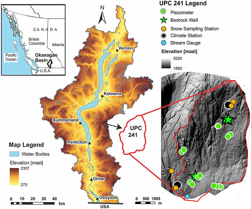
Figure 1. Okanagan Basin in British Columbia, Canada. The instrumentation at the Upper Penticton Creek (UPC) 241 watershed is shown overtop a LiDAR-derived bare earth image.

Mean daily temperatures in the catchment vary from −11.3°C in December to 19.2°C in July. Mean annual precipitation is 770 mm of which approximately 60% falls as snow. Late winter snow depths range between 1 and 1.5 m, and April 1 snow water equivalent (SWE) observed at a nearby long-term snow station, at 1,550 m asl, averaged 230 mm over the 1984–2018 period of record at UPC (Winkler et al., 2021). The snow disappears between the beginning of May and mid-June, depending on year and location at high vs. low elevation and in forested vs. clearcut sites. Peak streamflow occurs in May or June during snowmelt (April–June). Streamflow then declines through late summer and into the fall. The baseflow period is relatively long, extending from late fall through the winter until the onset of spring snowmelt.

Two long-term weather stations (Figure 1) have monitored rainfall, air temperature, surface and soil temperature, relative humidity, incident and reflected solar radiation, wind speed, snow depth and snow temperature year-round since August 1991 (Winkler et al., 2017). Snow surveys in 30-point grids have also been carried out at low (~1650 m asl) and high elevation (~1900 m asl) every 2 weeks from mid-March until the end of snowmelt. Streamflow has been measured at the Water Survey of Canada gauge site (08NM241; Figure 1) since 1984. A network of soil piezometers (Figure 1) measured shallow groundwater levels throughout the ice-free seasons of 2005–2010. Nine of the shallow piezometers were originally installed in 2005 as part of a study reported by Kuras et al. (2008), and six were added in 2007 (Voeckler et al., 2014). Moore et al. (2021) describes the instrumentation and datasets within the catchment.

In July 2007, three deep wells (two 30 m wells and one 50 m well) were drilled at UPC 241. Two of these wells are situated at high elevation and are ~3 m apart (wells W1 and W2), and one is at lower elevation (well W3) near the catchment outlet about ~2 km downgradient from the upper wells (Figure 1). No core was available as air rotary was used to drill the wells. Chip samples were collected and possible fracture locations were identified based on drilling resistance and changes in flow. The bedrock surface was within 0.5 m of the ground surface in W1 and W2. Granodiorite was encountered throughout the full well depth, with several small fractures intersected in both wells between approximately 6 and 24 m depth. Flow accumulated gradually down the boreholes, with the deepest fracture yielding the most water; the estimated yield of both wells is approximately 0.13–0.19 L/s. The bedrock was encountered at 4.5 m in W3 (also granodiorite over the full well depth) and cuttings at this depth were granular as opposed to competent chips, suggesting less competent rock. While some water was produced from several fractures (similar to W1 and W2), a major water-bearing fracture zone was encountered between 20 and 25 m; the estimated yield of this well is 0.76 L/s. The wells were completed as open boreholes with the exception of a cased interval that extends from the surface to ~1 m into the bedrock. Water levels in the three wells were monitored from 2007 to 2010; water levels continue to be monitored in W2 as this well is part of the BC Observation Well Network [OBS 387: (Province of BC., 2021)].

Materials and Methods

Lineament Data and LiDAR Data

Regional-scale lineaments were mapped throughout the Okanagan Basin using detailed aerial (ortho) photos and LANDSAT7 Thematic Mapper multispectral panchromatic imagery (near-infrared band 4). Additional details on how the data were processed are provided in Voeckler and Allen (2012).

Airborne LiDAR digital elevation data were acquired in August 2016 (zero snow cover) using a Reigl Q1560 scanner. The average point density for last returns was 10.33 m⁻², with a horizontal accuracy of 0.3 m and a vertical accuracy of 0.15 m, both reported at a 95% confidence interval. The DEM was delivered as a GeoTIFF file at a 1-m resolution.

Well Logging

A suite of borehole geophysical logs, including capacitive resistivity and normal resistivity, single point resistance, magnetic susceptibility, temperature, and full wave form sonic (tube wave amplitude and variable density), was acquired over a 2-day period in June 2009. Two logging runs were acquired; a down run (logging while the probe is going down the drillhole) and an up run (logging while the probe is coming up the drillhole). This procedure provided a means of evaluating the data quality and repeatability, while also acting as a check on any drift characteristics of the sensors. Measurements were acquired as frequencies and were converted into their respective quantitative units during subsequent processing. Selected logging results for W1 and W2 are discussed in Section Evidence of Fracture Zones From Lineament Mapping and LiDAR Data.

Pumping Tests

Short duration, constant discharge pumping tests were conducted at W1 and W3; step tests were done prior to determine optimum pumping rates for the constant discharge tests and are not discussed further herein. W1 was pumped at a constant rate of 0.06 L/s for 8 h (480 min). Then, the pump was turned off and the recovery response was monitored for 30 min (achieving ~ 90% recovery). Water levels were measured both in the pumping well, W1, and in the adjacent well observation well, W2. W3 was pumped at a slightly higher pumping rate of 0.08 L/s for ~8 h (480 min), with a 30-min recovery period. As there is no other well close to W3, no observation well data were obtained for this test. Drawdown was measured in each well using a pressure transducer datalogger as well as manually with a water level tape.

The pumping test data were analyzed using different analytical methods (e.g., Theis, 1935; Cooper and Jacob, 1946; Gringarten et al., 1975), and recovery data were analyzed using the Theis Recovery method (Theis, 1935) in order to calculate the hydraulic properties of the aquifer. The software AquiferTest Pro (Waterloo Hydrogeologic Inc., 2021) was used for the analysis.

Water Chemistry and Stable Isotopes

Water samples were collected from the groundwater wells (using a bailer at different depths), the soil piezometers, the stream at different locations, as well as from rainfall in summer 2007 and snow in winter 2008 (Figure 2). Temperature, pH, electrical conductivity (EC) and redox potential (Eh) were measured in the field. Half of each sample was filtered and acidified to a pH of 2 for cation analysis, while an un-acidified portion of sample was set aside for alkalinity titrations (average of 2–3 titrations), and the analysis of anions and δ²H and δ¹⁸O isotopes in water. Chemical analysis was done in the Geochemistry Lab in the Department of Earth Sciences at Simon Fraser University. Anion concentrations were measured using Ion Chromatography (IC) and major and minor cations using an Inductively Couple Plasma Atomic Emission Spectroscopy instrument (ICP-AES). Stable isotopes of oxygen and hydrogen in water were analyzed using a mass spectrometer at the Environmental Isotope Lab at the University of Waterloo.

FIGURE 2

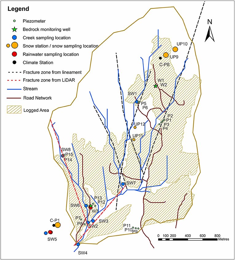
Figure 2. UPC catchment showing climate stations, snow stations, stream network, soil piezometers and groundwater wells where both physical water measurements were made as well as samples collected for water chemistry and stable isotope analysis. Logged areas shown in hatched brown. Also shown are presumed fracture zones mapped from lineaments (black dashed lines) and from the LiDAR-derived DEM hillshade (red dashed lines).

Numerical Modeling

MIKE SHE (Danish Hydraulic Institute (DHI), 2007) was used to simulate the hydrology of UPC 241. MIKE SHE is a fully distributed hydrologic modeling code that can simulate actual evapotranspiration (AET), overland flow, one-dimensional (1D) unsaturated flow, and three-dimensional (3D) variably saturated groundwater flow. Rivers, lakes, and other channels are simulated using the MIKE HYDRO River module (1D hydraulic model), formerly MIKE 11, which is coupled to the MIKE SHE model via link nodes. Further details on the comprehensive modeling capabilities of MIKE SHE can be found in the user manual (Danish Hydraulic Institute (DHI), 2007).

Conceptual Models

Four different conceptual models were developed for implementation in the numerical hydrological model (Figure 3). The base model (Model A) is essentially the same as that used by Voeckler et al. (2014), with some minor modifications as described below. This model consists of two soil layers overlying homogeneous fractured bedrock. The fractured bedrock is represented as an equivalent porous medium and extends to a depth of 220 m below ground surface. Model B introduces a network of large-scale vertical fracture zones within the bedrock, with a distribution as shown in Figure 2 (both the red and black fracture zones are included in the model). Model C introduces a 10-m thick weathered zone. Each of Models A, B and C use the original 30-m DEM to represent ground surface. Model D is identical to Model C, with the exception that the surface DEM is replaced by the LiDAR-derived DEM. All models, except Model B, have bedrock extending to a depth of 220 m. Model B has a greater depth (300 m) because if a shallower depth was used, the model dewatered; discussed further in Section Numerical Modeling.

FIGURE 3

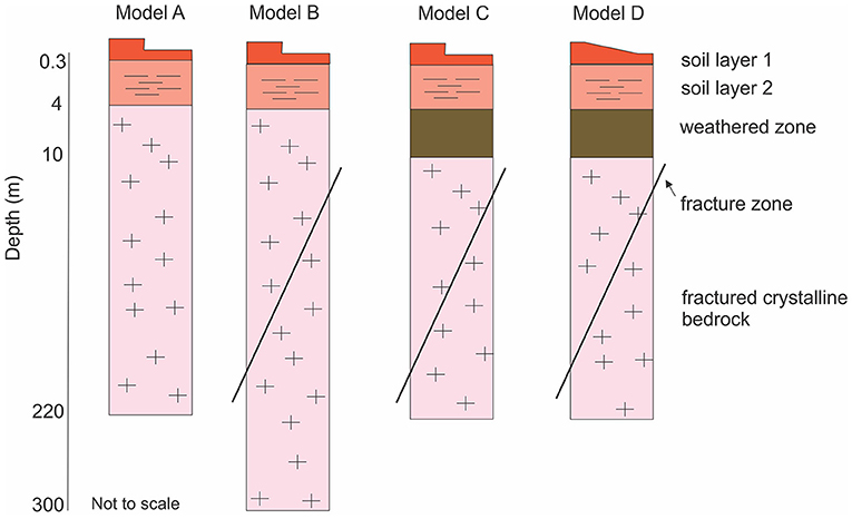
Figure 3. Schematic of the four conceptual models explored using a numerical hydrological model. (Model A) 2-layer soil zone overlying homogeneous bedrock to a depth of 250 m; (Model B) 2-layer soil zone, overlying heterogeneous bedrock (with fracture zones) to a depth of 300 m; (Model C) 2-layer soil zone, 10-m thick weathered zone, heterogeneous bedrock (with fracture zones); (Model D) 2-layer soil zone, 10-m thick weathered zone, heterogeneous bedrock (with fracture zones) with the ground surface based on the LiDAR-derived DEM.

Model Setup

The MIKE SHE model grid cells are discretized at a spatial resolution of 30 m. The model subsurface is divided into an unsaturated zone (UZ) and a saturated zone (SZ). The bedrock, weathered bedrock and fracture zones comprise the SZ. The UZ includes the various soil classes, bedrock and the weathered zone. The UZ and SZ overlap, so that the water table is free to move. In total, ten UZ soil profiles are defined based on soil class. Supplementary Figure 1A shows the soil zone map. The thickness of the upper soil layer (L1) is 0.3 m, and the thickness of the lower soil layer (L2) is variable (ranging from 1 to 4 m) as in Supplementary Table 1. The deepest soils (up to 4 m depth) are in the riparian zones at low elevation close to the stream outlet, while at higher elevations and where slopes are steep, the soils become thinner (Supplementary Figure 1B). One or two soil layers may be present above the bedrock (and weathered zone), depending on location in the watershed. If bedrock is exposed at surface, then no soil layers are defined, but a weathered zone is defined. The upper soil layers are discretized vertically into 0.2 m cells, and the bedrock into 0.5 m cells. In Models C and D, the weathered zone is also discretized into 0.5 m cells.

The model domain is the watershed boundary, which is defined as a closed boundary except at the stream outflow where it is open. The base of the model is assigned as a no flow (zero flux) boundary. Voeckler et al. (2014) simulated the exit of deep groundwater from the catchment using a specified flux equivalent to 2% of the catchment water balance, but they determined through sensitivity analysis that a flux of 1 or 0% did not appreciably affect the water balance. Therefore, for these models, a closed catchment (i.e., zero outward flux) is used. The hydraulic properties of the soils, bedrock, the fracture zones and the weathered zone are described below.

Hourly air temperature and precipitation (rain and snow) from the two climate stations (C-P1 and C-PB; Figure 2), over the period from October 1, 1990 to July 1, 2019, are used as input. Two climate zones are defined, with the border between them placed at roughly mid elevation within the watershed (Supplementary Figure 1C). A temperature lapse rate of −0.24°C/100 m is used to correct air temperature for elevation within each climate zone. The degree day method (Danish Hydraulic Institute (DHI), 2007) is used to simulate snowmelt with a melting temperature set to 0°C. The snow parameters are provided in Supplementary Table 3. Potential evapotranspiration (PET) was calculated using the Penman–Monteith method (Allen et al., 1998) in the software AWSET (Cranfield University., 2002) at daily time steps from the three meteorological data time series (precipitation, temperature and solar radiation) plus two additional time series data (hourly wind speed and humidity).

Land surface data includes seven different vegetation classes, representing the latest stage of logging in 2007 (47% of the watershed was clearcut logged) (Supplementary Figure 1D). Each vegetation class is assigned a representative leaf area index (LAI) and rooting depth. Supplementary Table 2 gives a description of the overstory, dominant height, LAI and rooting depth for each vegetation class (after Kuras et al., 2011). Where bedrock is exposed, the LAI is assigned a zero value.

The stream network and the channel cross sections are based on the DEM and survey data as described by Kuras (2006). The upstream ends of the stream branches are assigned as closed boundaries, whereas a water level boundary is assigned at the main outlet of the watershed using measured stream stage data. All other hydrodynamic parameters associated with overland flow and channel flow are provided in Supplementary Table 3.

Hydraulic Properties

The unsaturated zone hydraulic properties are provided in Supplementary Table 1. The values for the soils are the same values used by Voeckler et al. (2014). The weathered bedrock is included as a new soil class. The unsaturated hydraulic properties of weathered bedrock were estimated from literature values (Katsura et al., 2006) for weathered granite.

The saturated zone hydraulic properties include the bedrock, the weathered bedrock and the fracture zones (Supplementary Table 3). The bedrock properties were varied slightly from those used in the original calibrated model by Voeckler et al. (2014). In that original model, hydraulic conductivity (K) was assigned a K_horizontal = 3.2 × 10⁻⁷ m/s, with a K_vertical = 2.2 x 10⁻⁷ m/s, while in these models, K is isotropic with a value of 3.2 × 10⁻⁷ m/s because the anisotropy did not affect the model calibration and for granitic rock vertical anisotropy is unlikely. Specific storage (Ss = 1 × 10⁻⁵ m⁻¹) and specific yield (Sy = 0.01) were unchanged. The weathered zone was assigned K = 3.2 × 10⁻⁶ m/s, Ss = 1 × 10⁻³ m⁻¹ and Sy = 0.2.

The hydraulic properties of the fracture zones were estimated based on Voeckler and Allen (2012), who used inverse modeling to identify plausible parameter combinations of fracture zone properties to derive an estimate of “effective” fracture zone K that could be used in a watershed-scale model. They used the software FRED (Golder Associates Ltd., 2006) to set up a discrete fracture network (DFN) model to simulate the constant discharge pumping test at W3 (described above). They placed a discrete fracture in a cube domain (30 × 30 × 30 m) so that it would intersect W3 at a depth of 20 m. They noted that different simulations showed that changing the angle of the intersecting feature had no effect on the shape of the simulated drawdown curve. Thus, the fracture was given a nearly vertical dip and fully penetrated the model domain. Voeckler and Allen (2012) explored different combinations of fracture zone properties including the width, effective K, and compressibility. The matrix was assigned zero K (although non-zero values did not appear to change the simulation results). The overall tendency was that as the width was increased, the effective K and compressibility had to be lowered to maintain the model fit. The “best” match between the simulated drawdown and the measured drawdown in W3 was achieved using a fracture zone width of 5 m, K_effective = 1.1 × 10⁻⁶ m/s, and compressibility of 4.4 × 10⁻⁶ m²/N (Ss~0.04 m⁻¹).

Based on the DEM hillshade imagery, the fracture zones at UPC are definitely wider than 5 m; the damage zones appear to extend at least 30 m. Therefore, the K value from Voeckler and Allen (2012) was adjusted to 9.0 × 10⁻⁷ m/s and assigned to each 30-m wide fracture zone in the model. Specific storage and specific yield were the same as for the bedrock. We acknowledge that there is considerable uncertainty in the estimates of the fracture zone widths and their hydraulic properties. There is an unlimited combination of width and K_effective values that will lead to the same overall response. This is because, K_effective and effective width play off against each other in such a way as to maintain the effective fracture transmissivity (T_effective = K_effective × effective width).

Simulation Approach

The original model by Voeckler et al. (2014) was run at a daily timestep from 1994 to 2010. The initial groundwater levels in the saturated zone were set to ground surface, and so a model spin up period of roughly 10 years was needed for the groundwater levels to stop dropping and attain a dynamic equilibrium. Voeckler et al. (2014) calibrated the model using various datasets spanning 2005 to 2008: snow water equivalent, streamflow, pressure heads in the shallow piezometers, and groundwater levels in the wells. Data from 2009 to 2010 were reserved for model validation. For this study, the climate time series was lengthened, to start in 1990 and end in 2019, to allow for a longer streamflow and groundwater level (in W2) timeseries to be used for comparison with the simulated values. The observed data for snow water equivalent, pressure heads in piezometers and groundwater levels in W1 and W3 were the same as used by Voeckler et al. (2014) because monitoring ended in 2010. Climate, streamflow and groundwater levels in W2 continue to be monitored.

The four models were not re-calibrated. All parameters were maintained at the same values, with the exception of bedrock depth in Model B which had to be deepened to 300 m (rather than 220 m) because the model dewatered. This dewatering phenomenon is described in Section Numerical Modeling and in the Discussion.

Results

Evidence of Fracture Zones From Lineament Mapping and LiDAR Data

Figure 2 shows the location of four lineaments (black dashed lines) within UPC 241 that were mapped using orthophotos and Landsat imagery. These lineaments are inferred to be related to fracture zones. It is noted that UPC 241 is located in a region with relatively low lineament density within the Okanagan Basin; lineament density increases toward the central Okanagan valley (Voeckler and Allen, 2012), where the trace of the Okanagan Valley Fault Zone (a detachment fault), is under the Okanagan Lake and Okanagan Valley (Figure 1). The dips of these fracture zones cannot be determined based on the lineament data alone given that lineaments are visible as two-dimensional features on the landscape. The strike directions of the lineaments at UPC 241 are consistent with those mapped across the basin, and four different sets of lineaments were found to be statistically related to the four sets of fractures mapped in outcrop (Voeckler and Allen, 2012). Average dips for each of the four sets range from 11° to 58°.

Figure 4 shows the hillshade image for UPC 241 from the LiDAR data. Clearly evident is a network of elongated troughs (Figure 4A), which are interpreted to correspond to fracture zones (Figure 4B) where preferential erosion has taken place. Several of these troughs were identified in the lineament mapping (blue lines in Figure 4B), while two additional fracture zones in proximity to W3 (pink lines in Figure 4B), which were not detected by the lineament mapping, were subsequently identified in the hillshade image.

FIGURE 4

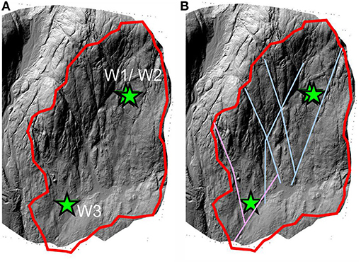
Figure 4. Hillshade image for UPC 241 showing (A) the location of the bedrock wells (green stars) and (B) the interpreted network of fracture zones (also shown in Figure 2).

Well Logging

Figure 5 shows selected geophysical logs for W1 and W3: magnetic susceptibility, capacitive resistivity, tube wave amplitude and full waveform log presented as variable density log (VDL). The magnetic susceptibility log is primarily used for lithology identification, but it can also be used to map alteration zones where magnetic minerals have been altered to non-magnetic minerals. If fluid flow occurs in porous or fractured rocks, it offers an oxidizing environment which may alter magnetic minerals to non-magnetic minerals and, therefore, show as lower magnetic susceptibility zones. Lower resistivity within a rock formation is often an indicator of a discrete fracture or fracture zone, since fracture are more porous (if open) and hence exhibit low resistivity (if water-filled). Variations in resistivity in crystalline rocks are primarily a function of pore water content and salinity. Low tube wave amplitudes are often exhibited by porous fractured rocks given their low density compared to unfractured rock.

FIGURE 5

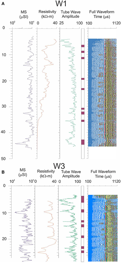
Figure 5. Magnetic susceptibility (MS), capacitive resistivity, tube wave amplitude and full waveform log presented as a variable density log for (A) bedrock well W1 and (B) bedrock well W2. The purple horizontal bars in the second last column represent interpreted fractures/fracture zones. Note that the logs for W2 are essentially identical to those for W1 given the close proximity of these wells (~3 m separation).

In W1, the zones of low resistivity, especially the ones below 30 m correlate well with the tube wave amplitude log and are indicated as low amplitude blue color zones in the VDL on the right of Figure 5A. The horizontal purple bars (second last column) indicate the fracture zones whose characteristics are depicted in the resistivity, susceptibility, and tube wave amplitude logs. At around 28 m, the resistivity is very low, but it is not indicated on the tube wave amplitude. The decrease of the tube wave amplitude in crystalline rocks has been correlated to permeable fractures, which suggests that the fracture zone around 28 m is not permeable. Note that the logs for W2 are essentially identical to those for W1 (not shown) given the close proximity of these wells (~3 m separation).

In W3, most of all the lower resistivity zones (Figure 5B) correlate very well with the tube wave amplitude log and are indicated as low amplitude, blue color zones in the VDL. Several fractures are identified (see fracture zone column). At shallow depth around 6 m, there is a large fracture zone about 4 m wide. In general, the fracture zones in W3 seem to have lower tube wave amplitudes than those in W1 (and W2), suggesting that the bedrock around W3 is more permeable. The differences in fracturing between the wells likely accounts for the variations in well yield. W3 has a relatively high yield at 0.761 L/s compared to W1 and W2 (0.13 and 0.19 L/s, respectively). If fracture intensity, as observed in these borehole logs, is assumed to be associated with proximity to a major fracture zone, then the low flow rates and the few fractures in W1 and W2 suggest that neither well is close to a major fracture zone, while W3, which appears to have wider and more frequent fracture zones, may be located closer to a major fracture zone.

Further evidence of the influence of significant fracturing at W3 compared to W1 and W2 is the borehole temperature logs (Figure 6). The temperature-depth profiles for W1 and W2 are virtually identical due to their close proximity, and the temperatures are virtually isothermal between 23 and 30 m, suggesting high vertical fluid flow rates in this zone, as illustrated by the orange inflow and outflow arrows on the graph. Temperature decreases slowly below 33 m depth. It is noted that fluid conductivity was relatively constant (20 μS/cm) above a depth of 32 m, but increased steadily with depth below 32 m, reaching 120 μS/cm at approximately 40 m depth. In W3, temperatures are significantly warmer than those in W1 and W2. W3 was flowing at the time of logging. This suggests there is at least one fracture zone at depth that has sufficient head to generate the flowing conditions, as represented by the green vertical arrow in the graph. However, there may be additional entry and exit intervals along this borehole.

FIGURE 6

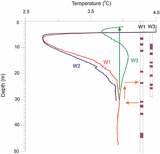
Figure 6. Temperature logs for W1, W2 and W3. Arrows indicate fluid flow (entry, upward flow, and exit). At the time of logging, W3 was flowing artesian, as represented by the vertical green arrow extending to surface. The purple horizontal bars represent the fractures/fracture zones interpreted from the resistivity and full waveform logs for each well as shown in Figure 5.

Pumping Tests

Figure 7 shows the log-log graphs of the head drawdown vs. time and the first derivative of drawdown with time for the two constant discharge tests conducted at UPC 241: one test at W1 with observations for W1 (Figure 7A) and W2 (Figure 7B), and the other test at W3 with observations for W3 (Figure 7C). Derivative plots, commonly referred to as diagnostic plots, were used to distinguish between different response types: 1) radial flow (flow is horizontal and radial toward the well) and 2) linear (flow is one dimensional and linear in a vertical plane toward the well) (Renard et al., 2009). Derivative plots can also be used to identify spherical flow and borehole storage.

FIGURE 7

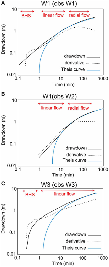
Figure 7. Log-log graphs showing the drawdown curve and the first derivative of drawdown with time along with the Theis curve for comparison for (A) the constant discharge test carried out in W1 with observations in W1; (B) the constant discharge test carried out in W1 with observations in W2 (3 m away); (C) the constant discharge test carried out in W3 with observations in W3. (BHS, Borehole Storage).

A uniformly fractured aquifer often has a radial flow response that can be represented by a classic This curve on a log-log plot (shown as the blue curves in Figure 7 for comparison) and the derivative of drawdown is constant (horizontal line) under radial flow conditions. A linear response is indicated by a more rapid initial response compared to Theis and the drawdown and its derivative are represented with straight lines on a log-log plot (Gringarten et al., 1975). Linear flow commonly occurs due to the presence of a vertical to sub-vertical discrete fracture (Gringarten et al., 1975) or wider fracture zone or dyke (Boehmer and Boonstra, 1987) that intersects, or is in close proximity to, the well (Allen and Michel, 1998). Borehole storage (BHS), which often occurs during pumping in low yielding rock units, is commonly identified on a log-log plot for the pumping well as a hump in the derivative plot at early time, and the drawdown curve has a slope of 1.

The analysis of pumping test data requires a conceptual model be identified based on the subsurface geological and the boundary conditions so that an appropriate analytical method can be selected for the analysis of the test data. The conceptual model for this study includes a network of vertical to sub-vertical fracture zones passing through a fractured bedrock unit. Based on the lineament mapping/LiDAR data and the borehole geophysics, one of these fracture zones is thought to pass close to W3. Accordingly, the possibility of linear flow influencing the pumping test at W3 was anticipated. Nevertheless, there may be other explanations for the responses to pumping at W1 and W3. The following is one interpretation. Other possibilities are explored later.

For the test at W1, drawdown data suggest a short period of BHS in the first min of the test (Figure 7A). During this time water is removed mostly from the borehole and not from the formation. Flow appears to be linear from 1 min to ~20 min. From 20 min to the end of the test at 480 min, the response appears radial (approximately a horizontal line in the derivative plot).

Figure 7B shows the test data for the observation well W2 during the pumping test in W1. Since W2 was not pumped, there is no BHS. The response is delayed slightly (by ~ 1 min) due to the 3 m separation of the wells. W2 also shows a brief period of linear flow from 1 to 20 min. Compared to W1, the radial flow period is much better defined in W2; the derivative curve is nearly horizontal.

Figure 7C shows the test data for the pumping test in W3. The drawdown curve and its derivative suggest BHS at the beginning of the test up to about one min. After that, linear flow dominates until the end of the test at 480 min.

The classical radial flow methods, Theis (1935) and Cooper and Jacob, 1946, were used to analyze the test data over the radial flow period in W1 and W2, and for the later portion of the test data in W3 despite radial flow not being observed in that test. Estimates of the hydraulic properties from both methods are shown in Supplementary Table 5. Note that storativity cannot be estimated for the pumping well. Hydraulic conductivity (K) is estimated by dividing transmissivity (T) by the representative aquifer thickness (here, the open hole interval is from the base of the well casing to the bottom of the borehole). Due to the interpreted linear response at W3, a linear flow model for pumping wells (Gringarten et al., 1975) was also used to analyze the pumping test data for W3. The entire curve was used in this analysis because it fit the data very well. The estimated properties from the Gringarten et al. methods represent the aquifer, not the fracture zone, so they can be compared with the Theis and Cooper-Jacob estimates.

The hydraulic properties from the pumping test results are very similar for W1 and W2, regardless of the analytical method used to analyze the data (Supplementary Table 5). K values range from 1.1 × 10⁻⁷ to 1.4 × 10⁻⁷ m/s. The K values calculated for W3 using the radial flow models range from 9.8 × 10⁻⁷ to 2.2 × 10⁻⁶ m/s. The Gringarten et al. (1975) method gave a K value of 1.1 × 10⁻⁶ m/s for W3. The recovery graphs are not shown, but the estimates of the hydraulic properties using the Theis Recovery method can be found in Supplementary Table 5. The results for the recovery tests are generally consistent, although the K values are very slightly higher in W1 and W2, and intermediate in W3 compared to the values from the pumping tests. Across all tests, the geometric mean K for W1 and W2 is 1.3 × 10⁻⁷ m/s and for W3 is 9.8 × 10⁻⁶ m/s.

The interpretation of pumping test data is often ambiguous because multiple conceptual models can give the same response. Uncertainties in our interpretation include 1) whether BHS occurs in the first min at both W1 and W3; 2) whether the linear response observed in W1 and W2 is due to a vertical/sub-vertical fracture intersecting those wells, or whether the response was influenced by the presence of W2 itself; and 3) whether the linear response at W3 is due to a nearby fracture zone or whether aquifer heterogeneity (e.g. a gradual decrease in K away from W3) causes the linear response. Ultimately, uncertainty in the interpretation of the pumping test data does not allow us to confirm that there are vertical / sub-vertical fractures influencing the tests; however, the high fracture intensity observed in the geophysical logs for W3 and the proximity of lineaments suggest that the conceptual model is reasonable.

Water Chemistry and Stable Isotopes

Supplementary Table 6 provides the water chemistry analysis results. Water chemistry parameters vary within a relatively small range as might be expected in this headwater catchment. The pH (2008 values) ranges from 5.8–7.3 (ave. 6.5). The redox potential (Eh) ranges from 337–602 mV (ave. 445 mV), even in the deep groundwater wells, suggesting contact with the atmosphere. The low electrical conductivity (EC) ranges from 34–144 μS/cm (ave. 59 μS/cm), reflecting the low total dissolved solids (TDS) of the waters, which ranges from 27–106 mg/L (ave. 51 mg/L).

Figure 8 shows a Piper plot of select water chemistry data for 2008, as well as for the bedrock wells in 2007. Most waters have a Ca-Mg-HCO₃ or Ca-Na-HCO₃ water type. Almost all samples plot in a close cluster on the Piper plot, except a few. For example, snow samples from UP9 and UP10 located at high elevation in the catchment have elevated SO₄ compared to CP-1 at low elevation. Although the TDS values are low for all snow samples so small differences in concentrations can be accentuated. P3 has elevated Na relative to the other soil piezometers. While P3 is among the deepest piezometers (~ 100 cm), it is not substantially deeper than the other ones (depths range from 55–119.5 cm). Piezometer P11, sampled on three consecutive days in summer 2008 (P11-1,−2,−3), showed increasing relative Na concentrations. Bedrock wells W1 and W2 sampled in summer 2007 shortly after drilling have slightly higher relative Na concentrations than the same wells sampled in 2008. Samples from W3 (depths of 21 m and 30 m) have a higher relative Na concentration as well as a higher EC (Ca and total alkalinity are the highest of all samples) compared to all wells and compared to the same well in 2008. Despite the varied sampling locations within the stream network (SW1-6), the water chemistry is very similar. Sites SW1, 2, 4 and 6 have a Ca-Na-HCO3 water type, while SW3 and SW5 have a Na-Ca-HCO3 water type.

FIGURE 8

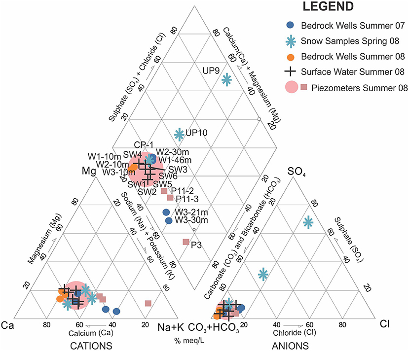
Figure 8. Piper plot showing major ion chemistry for waters sampled in the UPC241 catchment in 2007 and 2008. The locations of sampling points are shown in Figure 2.

Figure 9 shows a plot of δ¹⁸O vs. δ²H for samples collected in 2007 and 2008. Rain and snow samples were used to construct a local meteoric water line (LMWL). Three rain samples (shown on the inset plot in Figure 9) have less depleted values ranging from −6 to −10 ⁰/₀₀ for δ¹⁸O and −62 to −86 ⁰/₀₀ for δ²H (Supplementary Table 6), reflecting the higher temperature during summer. Snow samples have more depleted values (shown on both the main plot and the inset plot in Figure 9). In summer 2007, samples from W1 at three depths (12 m, 27 m and 46 m) plot close to each other, slightly above the LMWL, the single sample from W2 (30 m) is more enriched (and possibly affected by evaporation), and the samples from W3 at 30 m and W3 at 21 m have a more depleted isotopic composition. In summer 2008, W1 and W2 have similar isotopic compositions, while the sample collected from W3 when it was flowing artesian in 2008 is more depleted. There is some minor deviation of the isotopic composition of all three wells between 2007 and 2008. W1 and W2 were also sampled in winter 2008 (data not shown) and plot among the main cluster of samples on the graph, so, there does not appear to be a strong seasonal effect on the isotopic composition of the bedrock wells.

FIGURE 9

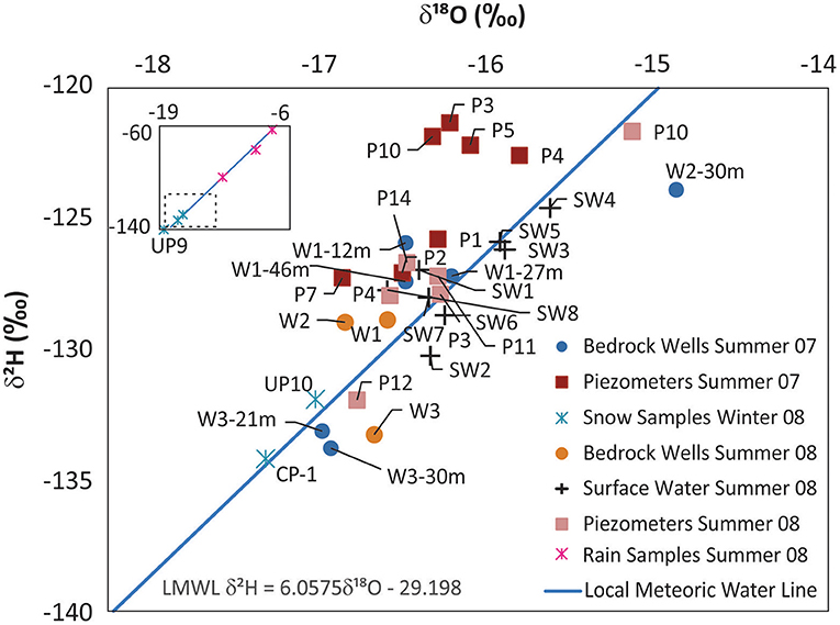
Figure 9. Plot showing δ¹⁸O versus δ²H for water samples collected at UPC241. The local meteoric water line (LMWL) was constructed from all snow and rain samples (shown in the inset plot; the main plot area is shown as a dashed rectangle on the inset plot).

The stream samples (SW1 to SW8) plot mostly along the LMWL, with SW4, SW5 and SW8 having slightly more depleted values despite their location at lower elevation in the catchment. SW5 is from the adjacent catchment UPC240 (see Figure 2). Soil piezometers P3, P4, P5 and P10 sampled in 2007 plot as a cluster above the LMWL with less depleted isotope concentrations compared to P1, P2 and P7. The variation in the isotopic composition does not appear to reflect logged vs. unlogged areas, elevation difference, or piezometer depth. Soil piezometers P3, P4 and P11 sampled in 2008 plot in the main cluster, while P12 plots lower on the line and P10 higher on the line. Interestingly, P12 is located nearby W3 in the valley at low elevation, and P10 is at moderate elevation (Figure 2).

Numerical Modeling

Figure 10 compares the observed and simulated groundwater levels in W2 and W3 over the full simulation period (October 1, 1990 to July 1, 2019). As mentioned in previously, W2 continues to be monitored, while data are only available for W3 from 2007 to 2010. Considering first the results for W2 (Figure 10A), the model spin up period is very different among the four models: Model A (1999), Model B (2009), Model C (1992), and Model C (1992). Models A, C and D are dynamically stable for a much longer period compared to Model B, which took a long time to spin up and arguably may not be dynamically stable even at the end of the simulation. The long spin up period for Model B is discussed later. Comparing the model fits for W2 near the end of the simulation (from 2014–2019), the simulated seasonal amplitude of the groundwater level is slightly overestimated in Models A, C and D. The average observed amplitude is approximately 7 m, while simulated amplitudes are slightly lower. The timing of peak and low groundwater levels is rather poorly simulated by all models. Observed groundwater levels rise rapidly in October due to fall rains, continue to rise gradually until peaking in June, and then decline over the summer, while the simulated groundwater levels begin rising in late July and peak in January. All of the models produce a visually good fit for W2, although less so for Model B.

FIGURE 10

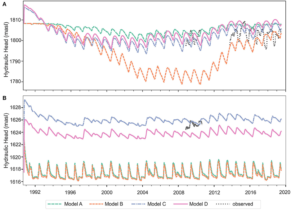
Figure 10. Observed and simulated groundwater levels in (A) W2 and (B) W3 for the period October 1, 1990 to July 1, 2019.

At W3 (Figure 10B), the simulated groundwater levels attain dynamic equilibrium very quickly, within about 5 years. This is because W3 is located at low elevation in the catchment where the water table is relatively shallow year-round. The four models, however, show very different average groundwater levels. Average annual groundwater levels are overestimated slightly in Model C, slightly underestimated in Model D, and greatly underestimated in Models A and B. The overall simulated seasonal amplitudes are similar among the four models, with slightly higher amplitudes compared to observed in Models A and B, and nearly identical amplitudes in Models C and D. The timing of the groundwater level responses is very close to observed for all models; however, the overall shape of the response in Models A and B is very peaked compared to the smoother observed response. Overall, Models C and D are much better at reproducing the groundwater level response in W3 than Models A and B, suggesting that the inclusion of the fractured zone and/or a weathered zone is important.

The model fit statistics for the period October 7, 2004 to October 6, 2019 for all observed data (W1, W2, W3, P1-P15, 4 snow stations, and streamflow) are provided in Supplementary Table 7. Four measures of fit are provided: root mean squared error (RMSE), normalized root mean squared error (NRMSE), R correlation, and Nash-Sutcliffe R², equivalently, the Nash-Sutcliffe Efficiency (NSE). The statistical fits for the various piezometers are mixed, varying from model to model for different piezometers. Total snow storage is very well fit at all four snow stations as is streamflow. Streamflow is overestimated by all models compared to observed streamflow by approximately 4% on an average annual basis. However, the model overestimation is primarily associated with peak flow overestimation in the months of April to June (or July). For the remainder of the months, streamflow is underestimated (as illustrated for Model D in Supplementary Figure 2). Overall, Models C and D are better at predicting the observed data than Models A and B.

Figure 11 compares the simulated depth to the top of the saturated zone (or water table) on June 18, 2010. Streamflow peaks in May or June at UPC 241, thus, June 18 represents a date when groundwater recharge would be high. The year 2010 was chosen because it is roughly midway between the end of the model spin up period and the end of the simulation. Positive numbers indicate that the water table lies above the top of the bedrock (i.e. within the soil zone), and negative numbers indicate that the water table lies at some depth in the bedrock. In all models, the depth to the water table is shallower along the streams at mid- to low elevation and surrounding the permeable vertical fractures. Presumably, because the fracture zones are closely associated with the stream network, the fractures zones may be important for maintaining baseflow in the streams during the summer. However, the water chemistry and stable isotope results for W3 are distinct from the stream samples, suggesting that a primary function of the fracture zones is the conveyance of water (i.e. snowmelt) from high elevation areas to lower elevation areas.

FIGURE 11

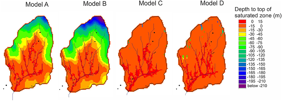
Figure 11. Simulated depth to the top of saturated zone on June 18, 2010 for Model A, Model B, Model C, and Model D.

The daily water balance values from MIKE SHE were summarized and output every 30 days, and then averaged annually according to water year (WY), which starts October 1 and ends September 30. The annual water balance results over a 5-year period (2005–06 to 2009–10) for all models are shown in Table 1. Only the main water balance components are reported; changes in canopy, snow, overland, unsaturated and saturated zone storage, river to groundwater, and error are excluded as the average values are generally low (< ~ 1%) compared to the other components, although they do account for discrepancies on an annual basis. Consequently, the water balance items do not necessarily total the precipitation. Precipitation (P) varied annually, from 690 mm in WY 2006-07 to 802 mm in WY 2005-06. Similarly, evapotranspiration (ET) varied interannually between the four models, but not substantially so, with average values ranging from 338 mm (45% of P) to 364 mm (49% of P). Overland flow (OL) flow to rivers also varied interannually and between models, with average values ranging from 299 mm (40% of P) to 363 mm (49% of P).

TABLE 1

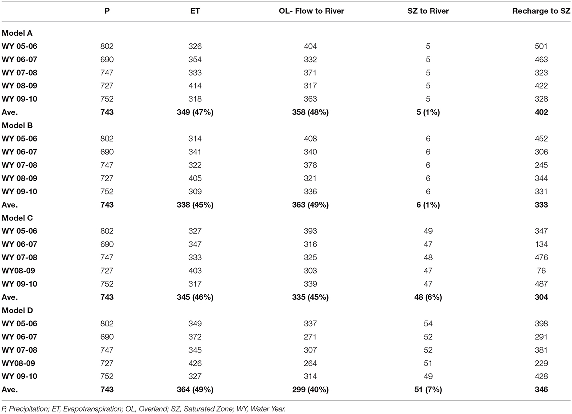
Table 1. Main water balance components (mm/year) for each individual water year (WY) and the WY average (Ave.) for 2005–06 to 2009–10. Values in brackets represent % of precipitation.

In the water balance, saturated zone (SZ) to river transfer, which is the groundwater contribution to baseflow, showed almost no interannual variability, but there was a significant difference between Models A and B with a SZ to river transfer of ~1% of P compared to Models C and D with 6–7% of P; Models C and D are the two with the weathered zone. In Models A and B, the simulated baseflow is ~1% of simulated streamflow, while in Models C and D, the baseflow is 14%. Thus, the weathered zone plays an important role in maintaining baseflow in the streams. Overall, the only significant difference between models was the groundwater contribution to baseflow.

Recharge is defined as the transfer of water from the unsaturated zone (UZ) to the SZ. Recharge is not included as part of the total water balance, but rather is included in the detailed water balance results for each of the UZ (reported as a loss of water) and the SZ (reported as a gain of water). Transfers occur daily and are summed for every cell of the watershed. So, if groundwater seeps at a cell where the water table intersects the ground surface, and then water flows overland, only to enter the unsaturated zone at another cell, this would be counted as recharge. Consequently, the annual recharge numbers are misleading. Shown in Table 1 is the net annual recharge (the sum of the positive and negative numbers); the average recharge for all water years ranges from 304 mm (Model C) to 402 mm (Model A). Clearly, the numbers far exceed plausible recharge because the sum of ET, OL flow to river and SZ to river together make up 95–97% of the water balance. Thus, OL flow to river and recharge to SZ interact and cannot be clearly distinguished from each other.

Figure 12 compares monthly recharge for the year 2010 for the four models; also shown is total monthly precipitation. Positive recharge numbers indicate that water is transferred from the UZ to the SZ (true recharge), while negative numbers indicate a transfer from the SZ to the UZ. All models have consistent timing of recharge, initiating in either May or June, reaching a peak in July or August, and then declining, such that by October or November, recharge is negative. Models A and B (with no weathered zone) have high negative recharge through the late fall and winter, suggesting that there is significant transfer of water from the SZ to the UZ during this time. Once a weathered zone is introduced (Models C and D), significantly much less water is transferred back to the UZ. The abrupt change in hydraulic properties at the weathered zone – bedrock boundary, which is anywhere from 10 m to 14 m depth depending on soil thickness, likely accounts for the lower transfer. Interestingly, the weathered zone – bedrock contact depth coincides with the minimum historical groundwater level in W2 (~ 13 m). Therefore, the transition between the SZ and UZ, at least a higher elevation in the watershed, is occurring near this contact. Additionally, the high precipitation rates in November, December and January do not translate into any recharge, although water is being added to subsurface storage during these months (not shown in the annual water balance). This means that water is infiltrating the UZ and adding water to storage, but the water has not yet percolated deep enough to reach the water table; therefore, no recharge is recorded in the model.

FIGURE 12

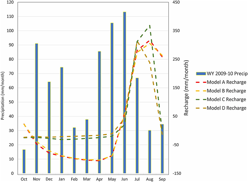
Figure 12. Precipitation and simulated recharge for Models A, B, C and D for water year (WY) 2009–2010.

Discussion

So, how important are the fracture zones? To answer this question requires some clarification of which fracture zones? Our original interpretation of the presence of fracture zones was inferred from lineaments mapped from LANDSAT data and orthophotos. Because approximately 50% of the watershed was tree covered at the time the lineament mapping was done, it was difficult to identify lineaments in heavily treed areas. The lineament mapping identified four fracture zones (black dashed lines in Figure 2), but none are in close proximity to any of the wells. Only recently did the LiDAR bare earth imagery become available (Figure 1). Several of the linear features on that image coincide with the mapped lineaments, but two dominant features passing through the lower catchment do not, and thus, these two features were added to the fracture zone map (red dashed lines in Figure 2). Neither fracture zone passes through W3, but they intersect south of the well.

At the outset of the field study, there was some evidence of well W3 being located in proximity to a fracture zone. The well is located at low elevation in catchment, within the valley bottom, and is fairly close to the main stream channel. These two conditions alone would suggest that W3 might be influenced by a fracture zone, because stream channels in mountainous terrain commonly follow zones of weakness in the bedrock, which have eroded over time to create the stream channels themselves. During drilling, water was produced at relatively shallow depth and the estimated well yield was much higher compared to W1 and W2. The borehole geophysical data confirmed that W3 is more intensely fractured compared to W1 and W2. However, this alone does not necessarily suggest that a fracture zone may be nearby. The linear flow response in W3 is interpreted to be due to a vertical to sub-vertical fracture zone in proximity to the well, but there may be alternative interpretations of the test data, such as a gradual decrease in fracture intensity away from the well. The dominantly radial flow conditions for the test at W1 suggest that the bedrock near W1 and W2 (and presumably across the catchment) can be approximated by an equivalent porous medium with properties that reflect a reasonably uniform distribution of fractures. It is for this reason that a homogeneous bedrock layer was used in Model A. Models B, C and D also assume the bedrock can be represented as an equivalent porous medium, and likewise the fracture zone themselves, although the bedrock as a whole would be conceptualized as heterogeneous.

The water chemistry and stable isotope data hint at a potentially different flow path for water entering W3. In 2007, the Na and Ca and total alkalinity concentrations were higher in W3 (W3-21 m and W3-30 m) compared to W1-46 m and W2-30 m, as was the relative Na concentration (Figure 8). One could speculate that the higher relative Na might be due to cation exchange, which could be taking place on clay minerals formed during weathering of the granitic rock. Additionally, the Na, Ca and total alkalinity were also higher in the W3 samples than in any other sample, suggesting that more weathering is taking place near W3 compared to other locations in the watershed. Enhanced weathering would likely occur within the fracture zones. The isotope results indicate a meteoric origin for all waters in the catchment, with most samples plotting as a cluster closer to the isotopic composition of the snow rather than rain, suggesting a dominantly snowmelt origin (Figure 9. However, the rain samples were collected during the summer – hence their more enriched composition. Fall or spring rains may not be as enriched due to cooler temperatures. Interestingly, samples collected in the valley (W3 and P12) consistently have more depleted values, suggesting a higher relative snowmelt contribution compared to the other samples. Because the valley receives water from the entire catchment and the catchment hydrology is snowmelt dominated, the depleted isotopic composition at W3 might be anticipated. Whether the isotopic composition is evidence of a fracture zone influencing this well is uncertain.

Varying the model structure highlighted some differences in both model performance and the catchment water balance. No single model outperformed the others, although Models C and D (with fracture zones and a weathered zone) are considered to be more robust, due to their shorter spin up times and generally better fit statistics, particularly for W3. The streamflow fit statistics were very similar as were the snow fits. The fits for the piezometers varied considerably among the models, pointing to the challenges of reproducing hydraulic responses at discrete point in a landscape with varying soils, vegetation type, vegetation presence, etc.

One interesting outcome was the need to deepen the bedrock depth in Model B. This is the model that introduced only the fracture zones (no weathered zone). Because the initial condition has the water table at ground surface, some spin up period is needed for the model to reach some dynamic equilibrium, whereby the water table is no longer dropping. The original model by Voeckler et al. (2014) required approximately 10 years for the model to spin up. In this study, Model A similarly required approximately 10 years (dynamically stable conditions attained in 1999) because it is essentially the same as the model by Voeckler et al. (2014). Model B required a long spin up time (until 2009), and Models C and D required relatively short model spin up times (until 1992). Model B could not be run with a bedrock depth of 220 m because the water level continuously dropped, causing the simulation to terminate. A depth of 300 m was the minimum depth required for a successful run. The cause of dewatering is assumed to be related to the high hydraulic conductivity of the fracture zones, which likely causes the water to drain from the fracture zones more rapidly than the water can be replenished; if the water level drops to the base of the model anywhere in the domain, the model terminates. The addition of a weathered zone above the fractured bedrock eliminated the need to deepen the model to avoid dewatering. Thus, the weathered zone is considered to be an important element of the model structure.

There was not much difference in the water balance between Models C and D. Model D, with the LiDAR-derived DEM used for ground surface, had slightly higher evapotranspiration (49% of precipitation) compared to Model C (46% of precipitation); lower overland flow to river (40% compared to 45%), slightly more saturated zone to river transfer (7% compared to 6%), and an overall higher transfer of water from the unsaturated zone to the saturated zone on an average annual basis. Thus, the LiDAR-derived DEM generated slightly more recharge. The greater spatial resolution in topography in Model D, compared to the coarser 30-m DEM used in Models A to C), potentially allows more water to collect in small topographic depressions, causing ponding and then infiltration.

All of the models carry uncertainty, both in terms of overall model structure (e.g. Beven, 2005; Gupta and Govindaraju, 2019; Moges et al., 2021) and the parameters themselves (Beven and Binley, 1992). However, only four variations of the model structure were explored in this study. Additional variations in model structure / parameterization could include: 1) varying the widths and hydraulic properties of the fracture zones. In this study the fracture zones were all assigned the same width (30 m) and uniform hydraulic properties based on estimates from Voeckler and Allen (2012); 2) varying the depths of the fracture zones. In this study the fracture zones were modeled as fully penetrating the bedrock (to the base of the model domain); however, they may terminate variably at shallower depths; 3) including other possible fracture zones. In this study, not all of the potential fracture zones visible in the DEM hillshade imagery (Figure 1) were included; 4) varying the thickness of the weathered zone and its properties. The weathered zone was assigned a uniform depth of 10 m and hydraulic properties estimated from the literature; however, the weathered zone can be expected to be variable across the catchment; and 5) representing the bedrock as a discretely fractured medium. In this study the bedrock was assumed to be an equivalent porous medium, when in reality there are discrete fractures that may or may not be uniformly distributed and connected.

Ultimately, all of the models are considered plausible and gave reasonable results in terms of similarity in overall fit to observed data (snow, streamflow, pressure heads in piezometers, and groundwater levels) and water balance results. Models C and D, which included both a weathered zone and fracture zones, are considered the “best” models. A more rigorous uncertainty analysis to explore finer scale variations in model structure and fracture zone parameterization may provide greater insight into the relative significance of fracture zones in catchment scale groundwater flow processes.

Conclusions

The main goal of the study was to determine the hydrological importance of fracture zones, recently identified in a LiDAR-derived DEM hillshade, that pass close to a deep groundwater well (W3) located in the valley bottom of a small snowmelt-dominated mountain headwater catchment. More intense fracturing in W3, compared to two wells at higher elevation (W1 and W2), was revealed in a suite of borehole geophysical logs. W3 also exhibited a linear flow response during a pumping test, which was interpreted to be related to the presence of a nearby sub-vertical fracture zone. The major ion chemistry and stable isotope composition reveal only a slightly different chemical composition and a more depleted isotopic signature for W3 compared to other groundwaters and surface waters sampled throughout the catchment. To explore the potential role of these fracture zones on the catchment hydrology, an integrated land surface – subsurface hydrologic model was refined in steps, beginning with a single homogeneous bedrock layer, and progressively adding 1) a network of large-scale fracture zones within the bedrock, 2) a weathered bedrock zone, and 3) an updated digital elevation model based on the LiDAR.

Collectively, there is evidence of a fracture zone(s) near W3. However, the catchment scale modeling results (model fit and water balance) for the sequence of four models are relatively similar, suggesting that all models are plausible. However, the models with a weathered zone appear to perform better. Unfortunately, the model including only the fracture zones was difficult to spin up due to dewatering, which may have influenced the results. Additional simulations to vary the model structure and parameterization may provide greater insight into the relative role of the fracture zones and the weathered zone.

Data Availability Statement

Publicly available datasets were analyzed in this study. This data can be found here: Zenodo repository, https://doi.org/10.5281/zenodo.4456139. Water chemistry and stable isotope data are provided in Supplementary Materials.

Author Contributions

DA: conceptualization, methodology, writing-original draft preparation, supervision, and funding acquisition. DA and AN: formal analysis, investigation, and writing-review and editing.

Funding

This research was supported by a Natural Sciences and Engineering Research Council of Canada (NSERC) Discovery Grant to DA.

Conflict of Interest

The authors declare that the research was conducted in the absence of any commercial or financial relationships that could be construed as a potential conflict of interest.

Publisher's Note

All claims expressed in this article are solely those of the authors and do not necessarily represent those of their affiliated organizations, or those of the publisher, the editors and the reviewers. Any product that may be evaluated in this article, or claim that may be made by its manufacturer, is not guaranteed or endorsed by the publisher.

Acknowledgments

We acknowledge the following individuals: CJ and AL Mwenifumbo from the Geological Survey of Canada, who carried out the borehole geophysical logging and processed the data; Natural Resources Canada who provided the lineament data; H. Voeckler who undertook the original hydrological modeling as part of his Ph.D. research at the University of British Columbia; R. Winkler formerly at the BC Ministry of Forests, Lands, Natural Resource Operations and Rural Development (FLNRORD) for collecting the snow samples for isotopic analysis and providing access to the LiDAR data; D. Kirste from Simon Fraser University who assisted with the field chemistry sampling program.

Supplementary Material

The Supplementary Material for this article can be found online at: https://www.frontiersin.org/articles/10.3389/frwa.2021.767399/full#supplementary-material

References

Allen, D. M., and Michel, F. A. (1998). Evaluation of multi-well test data in a faulted aquifer using linear and radial flow models. Ground Water. 36, 938–948. doi: 10.1111/j.1745-6584.1998.tb02100.x