 Alexander VanDeWeghe
 Victor Lin2
 Jennani Jayaram
 Andrew D. Gronewold
- 1Department of Civil and Environmental Engineering, College of Engineering, University of Michigan, Ann Arbor, MI, United States
- 2Department of Electrical Engineering and Computer Science, College of Engineering, University of Michigan, Ann Arbor, MI, United States
- 3Department of Mathematics, College of Literature, Science, and the Arts, Ann Arbor, MI, United States
- 4School for Environment and Sustainability, University of Michigan, Ann Arbor, MI, United States
Understanding impacts of climate change on water level fluctuations across Earth's large lakes has critical implications for commercial and recreational boating and navigation, coastal planning, and ecological function and management. A common approach to advancing this understanding is the propagation of climate change scenarios (often from global circulation models) through regional hydrological models. We find, however, that this approach does not always fully capture water supply spatiotemporal features evolving from complex relationships between hydrologic variables. Here, we present a statistical approach for projecting plausible climate-related regional water supply scenarios into localized net basin supply sequences utilizing a parametric vine copula. This approach preserves spatial and temporal correlations between hydrologic components and allows for explicit representation and manipulation of component marginal and conditional probability distributions. We demonstrate the capabilities of our new modeling framework on the Laurentian Great Lakes by coupling our copula-derived net basin supply simulations with a newly-formulated monthly lake-to-lake routing model. This coupled system projects monthly average water levels on Lake Superior, Michigan-Huron, and Erie (we omit Lake Ontario from our study due to complications associated with simulating strict regulatory controls on its outflow). We find that our new method faithfully replicates marginal and conditional probability distributions, as well as serial autocorrelation, within and among historical net basin supply sequences. We find that our new method also reproduces seasonal and interannual water level dynamics. Using readily-available climate change simulations for the Great Lakes region, we then identified two plausible, transient, water supply scenarios and propagated them through our model to understand potential impacts on future water levels. Both scenarios result in an average water level increase of <10 cm on Lake Superior and Erie, with slightly larger increases on Michigan-Huron, as well as elevated variability of monthly water levels and a shift in seasonal water level modality. Our study contributes new insights into plausible impacts of future climate change on Great Lakes water levels, and supports the application and advancement of statistical modeling tools to forecast water supplies and water levels on not just the Great Lakes, but on other large lakes around the world as well.
1. Introduction
The Laurentian Great Lakes watershed is home to more than 40 million inhabitants (MacKay and Seglenieks, 2013) and has a surface area of roughly 244,000 km2 (Moukomla and Blanken, 2016), the largest of any lake system on Earth (Gronewold et al., 2013b). Regional ecological health and economic security are closely interwoven with this system, in large part because of the capacity of the Great Lakes to support diverse habitats (Cvetkovic and Chow-Fraser, 2011), commerce (Millerd, 2011; Meyer et al., 2016), and recreation (Nevers and Whitman, 2011; Gronewold et al., 2013c). The capacity of the Great Lakes to support these activities is, in turn, dependent on historical and future water quantity and quality dynamics (Mortsch and Quinn, 1996), including (but not limited to) those associated with coastal water level variability (Mortsch and Quinn, 1996; Gronewold and Stow, 2014a). Given the great economic and ecological value of the Great Lakes, and recognizing the potential risks associated with ongoing climate change (Pryor et al., 2014), understanding plausible future water level dynamics on the Great Lakes is paramount. Indeed, Great Lakes scientists have undertaken this very endeavor for decades (Quinn, 1978; Croley, 1990; Angel and Kunkel, 2010).
Previous attempts to quantify shifts in the Great Lakes hydrologic cycle reflect the role that climate change has already been playing across the region (Marchand et al., 1988; Quinn, 2002). Some of these historical projects, many of which have come under scrutiny (Lofgren and Gronewold, 2013), focused on translating that understanding into seasonal and interannual water supply forecasting systems using a “change-factor” method (Croley, 1990) based on output from a chain of lake thermodynamics and rainfall-runoff models collectively known as the Advanced Hydrologic Prediction System, or AHPS (Gronewold et al., 2011). This modeling framework (Croley, 1990) was subsequently adopted in a range of climate impact studies (Hartmann, 1990; Hayhoe et al., 2010). Importantly, some of these studies employed a perturbed time series of historical data (using either a multiplication factor, or ratio, based on separate climate modeling results) as future forcings. These forcings were intended to be representative of a future climate.
The perturbed climate data became input for the AHPS, which translated climate variables such as daily temperatures, precipitation, and humidity into water supply components (also commonly referred to as a “net basin supply,” or NBS). More specifically, NBS in the Great Lakes is typically defined as the sum of terrestrial runoff into each lake, and net atmospheric water supply (precipitation minus evaporation) over the surface of each lake (Mailhot et al., 2019). This value is typically expressed as a height of water over each lake surface (Music et al., 2015). Due to the large surface area of the Great Lakes relative to basin size, overlake precipitation, overlake evaporation, and runoff have similar annual magnitudes, but very different seasonal dynamics (Lenters, 2001; Gronewold et al., 2013a).
Despite variation in emission scenarios considered across previous studies (Music et al., 2015), those (most of which were published prior to 2010) that employed the Croley (1990) methodology predicted substantial decreases in both NBS and water levels on the Great Lakes (Lofgren, 2004). Lofgren et al. (2011) and Lofgren and Rouhana (2016) subsequently identified methodological flaws in the estimation of evapotranspiration in the AHPS core runoff model (the large basin runoff model, or LBRM), leading to arguably biased formulations of runoff and NBS resulting from the use of near-surface air temperature as a proxy for potential evapotranspiration (Milly and Dunne, 2017). Furthermore, application of the change-factor method only represents shifts in mean, and later variance, of hydrological components. This method does not fully account for the full probability distribution underlying each water balance component (Music et al., 2015). Correctly representing evolving solar radiation dynamics in relatively simple models that simulate the hydrologic impacts of climate change (Lofgren et al., 2013) is just one challenge facing the Great Lakes water resources planning community.
There are other challenges, however, associated with more contemporary methods that utilize hydrological output directly from global circulation models (GCMs). Manabe et al. (2004), for example, utilized a GCM to demonstrate that water rich regions of North America, such as the Great Lakes basin, would experience a significant increase in runoff and outflow, suggesting a parallel increase in water level. However, GCMs typically lack the regional specificity necessary to reflect climate interactions at the scale of a lake system (Music et al., 2015; Briley et al., 2021); some models grossly misrepresent or even simply don't include critical lake-atmosphere interactions that affect the regional climate and propagate into meteorological phenomena (Wright et al., 2013; Bryan et al., 2015; Fujisaki-Manome et al., 2017). Other regional processes such as soil and vegetation interactions and rainfall over small watersheds can have a significant cumulative effect on water availability, but are similarly misrepresented, or even neglected, in GCMs (MacKay and Seglenieks, 2013).
An alternative approach that has gained popularity in recent years is downscaling GCM results with regional climate models (RCMs), often coupled to a lake-atmosphere model (Gula and Peltier, 2012; MacKay and Seglenieks, 2013; Music et al., 2015; Notaro et al., 2015; Mailhot et al., 2019). Studies utilizing RCMs have demonstrated the possibility for much more varied results than had previously been considered under the “change-factor” method (Winkler, 2015). MacKay and Seglenieks (2013), for example, projected single digit centimeter declines in water levels, while Notaro et al. (2015) projected both large increases in water level (+42 cm on Michigan-Huron) using one regional model (RCM-CNRM), as well as significant decreases (−29.6 cm on Michigan-Huron) using a different regional model (RCM-MICROC5). These findings underscore the substantial variability that either different RCMs, or that different parameterizations within a given RCM, can introduce. In contrast, studies using ensembles of multiple RCMs to project hydroclimate scenarios resulted in less extreme changes in average water supply. Most recently, a study of 28 climate simulations under five RCMs predicted only small increases in average NBS across the basin, but projected an amplification of the seasonal NBS cycle driven by increases in both precipitation and evaporation (Bartolai et al., 2015; Mailhot et al., 2019).
To provide more robust simulations of plausible NBS time series under climate change scenarios, we introduce a methodology utilizing a parametric regular vine copula to predict monthly NBS component values given a hypothesized change or trend in each component. Copulas are multidimensional cumulative distribution functions (CDFs) that originate from marginal CDFs (Schölzel and Friederichs, 2008; Laux et al., 2011; Lee and Salas, 2011; Maity, 2018). More specifically, copulas encode relationships between some number (e.g., d) of marginal probability distributions (in our case, for d hydrological variables) and a new d-dimensional joint probability distribution that preserves serial and cross-correlation.
As such, copulas represent an efficient tool for simulating long-term environmental variables that are highly correlated across space and time. Previous studies have shown that copula models have the potential to successfully represent these dependencies (Pouliasis et al., 2021). Other conventional (and perhaps more common) statistical models in water resources research, such as autoregressive, fractional Gaussian noise, and non-parametric models, have the potential to misrepresent (or even not represent at all) them (Lee and Salas, 2011). Here, we utilize a specific type of copula, referred to as a “vine” copula, which constructs the multivariate joint distribution using a series of bivariate relationships (rather than a single dependence structure across all variables simultaneously).
Prior studies have also, more specifically, evaluated the efficacy of copulas in capturing hydroclimate phenomena on other large bodies of water, suggesting that hydrologic behavior can plausibly be modeled using copulas (Lee and Salas, 2011; Latif and Mustafa, 2020; Pouliasis et al., 2021; Zaerpour et al., 2021). However, many conventional copulas (such as Frank, Clayton, and Gumbel) are prohibitively complex at higher dimensions (Lee and Salas, 2011). While Gaussian and student's-t copulas can accommodate joint distributions of many dimensions, we focus our attention on vine copulas to allow for uniquely structured bivariate dependencies such as heavy tail weighting, multimodality, and physical boundary conditions.
Likewise, it is advisable to use regular vines under certain circumstances in which the dependence structure of the variables is unclear, a condition reflected in the high number of monthly NBS component variables across the Great Lakes (Latif and Mustafa, 2020). With this in mind, we are able to use vine copulas to capture overarching variable interactions while simultaneously managing all constituent pairwise dependencies.
Therefore, the approach we introduce intends to leverage the strength of regular vine copulas to capture spatial and temporal distributional dependencies between monthly NBS components for large lakes and, in particular, for each of the Laurentian Great Lakes. We couple these statistically robust NBS simulations with a lake-to-lake routing model utilizing monthly stage-fall discharge equations. Monthly outflow models (as opposed to annual-scale models often used in multi-decadal simulations) allow us to represent seasonal variability in water supplies evolving from factors such as ice cover and vegetation. We demonstrate the utility of this methodology by simulating historical and future water levels under two plausible hydroclimate scenarios that represent a continuation of observed NBS component trends, and a blending of existing trends with RCM NBS change projections. We use these water level simulations to assess three metrics of water level behavior: long-term average, seasonality, and frequency of extreme values.
2. Methods
2.1. Copula Calibration
We began by extracting historical water balance data for the Great Lakes using archived output (Do et al., 2020a) from the Large Lake Statistical Water Balance Model (L2SWBM) (Gronewold et al., 2020). The L2SWBM utilizes a Bayesian framework (Press, 2003; Gelman et al., 2004) to assimilate independent hydrological data products across the Great Lakes and subsequently infer the “true” monthly value for each water balance component. Although these monthly values are ultimately unknown, the L2SWBM is constrained by a traditional water balance equation, and uses multiple data sources to develop prior and likelihood functions for each component. Thus, the posterior estimates of the L2SWBM reconcile observed (or simulated) values from independent data products to close the water balance of the entire hydrologic system (Gronewold et al., 2016).
For this study, we specifically extracted median NBS component values from the L2SWBM to calibrate the copula. We calibrated the copula model as a “Regular Vine” copula within the RVineStructureSelect() function in the VineCopula package (Nagler et al., 2021) in the R statistical software program (R Core Team, 2017). We converted our 70 year NBS component observations into pseudo-observations which are both readable by the RVineStructureSelect() function, and rank-normalized to the interval [0,1]. The RVineStructureSelect() function then optimally generates a maximum spanning tree with edge weights as the correlation of pairs of variables amongst the 108 variables (3 lake systems × 3 water balance components × 12 months). Likewise, the RVineStructureSelect() function assigns them to the most appropriate bivariate copula family.
We then used the RVineSim() function to generate simulated values for each lake water balance component. We used quantile functions to map component values from [0,1] space into “real” values. The marginal distributions for each water balance component were, following previous protocols established in developing the L2SWBM (Gronewold et al., 2016, 2020; Do et al., 2020b), prescribed as three-parameter gamma, Gaussian, and log-normal for precipitation, evaporation and runoff, respectively. The three-parameter gamma distribution is parameterized using the same shape and scale parameters as a conventional gamma distribution along with an additional shift parameter. As described in the following sections, this approach allows us to propagate plausible climate change scenarios through changes in the parameters of each probability distribution.
2.2. Outflow and Routing Model
To propagate the monthly water balance components generated by the copula into simulated monthly water levels, we developed an outflow model to capture flow dynamics between the lakes. Specifically, we encoded a conventional stage-fall discharge (SFD) equation, which simulates lake outflow as a function of water surface elevation in an upstream and (in some cases, depending on the extent of backwater effects) downstream lake (Gessler et al., 1998; Schmidt and Yen, 2008; Westerberg et al., 2011; Apps et al., 2020). SFD models are particularly prevalent in the Laurentian Great Lakes, where they have been used for decades in long-term water level simulation studies and operational forecasting systems (Brunk, 1968; Quinn, 1978; Labuhn et al., 2020; Quinn et al., 2020; Thompson et al., 2020).
To simulate outflow (Q) from Lake Michigan-Huron, we used the following SFD formulation with both stage and fall components to accommodate the effects of backflow through the Detroit and St. Clair Rivers.
where z2 and z1 represent upstream and downstream lake elevations, respectively, and zsill represents a constant lake “sill” elevation (roughly analogous to the elevation of the channel bottom). Model coefficients are represented by a, b, and c, where a subscript m indicates that a coefficient is allowed to vary seasonally. This approach allows our models to account for monthly changes in the relationship between water levels and channel flow which result from factors such as channel vegetation and ice cover (Derecki and Quinn, 1986; Lu et al., 1999).
To simulate outflow from Lake Superior and Lake Erie, we used (following conventional protocols) the following simplified SFD model (superscripts are added to differentiate flow values and coefficients derived from the simplified SFD model; subscripts differentiating models for Lake Superior and Lake Erie are removed for clarity):
Taking the logarithm of each formulation leads to the following linear models:
where ϵ and ϵ′ are model error terms.
We then conducted a Bayesian analysis to estimate model coefficients using historical Great Lakes beginning-of-month water level measurements, and monthly average flow measurements, as data (i.e., for z2, z1, and Q). We obtained this data from publicly-available archives maintained by the National Oceanic and Atmospheric Administration (NOAA) Great Lakes Environmental Research Laboratory (Smith et al., 2016), and originally developed by the Coordinating Committee on Great Lakes Basic Hydraulic and Hydrologic Data (Gronewold et al., 2018).
2.3. Climate Scenario Selection
To demonstrate the utility of our water level forecasting framework, we evaluated three 50-year water supply scenarios. The first scenario is a “baseline” scenario, executed without any perturbation of the original copula water balance component parameters. We then developed and evaluated two additional 50-year water supply projections, each developed under different climate-perturbed water supply conditions. The historical baseline simulation will hereafter be referred to as SC1. After comparing our baseline scenarios and historical observations to ensure a minimal bias, we then base our analysis on an intercomparison between our three model simulations. This approach minimizes the impacts of any potential biases (which we attempt to minimize through model calibration) in our historical simulations (Frigon et al., 2010).
While most multidecadal Great Lakes water level forecasts acknowledge the impact of climate change on future water level regimes, there has not been a focus on identifying and propagating existing climate change signals directly into future water supply scenarios (Notaro et al., 2013, 2015; Lofgren and Rouhana, 2016). Instead, water levels are typically simulated under future emissions or temperature change scenarios, but those scenarios are sometimes inconsistent with observed trends in NBS components. To address this shortcoming in conventional regional water supply forecasting, we identify significant trends in NBS components from 1950 to 2019 to inform our first plausible climate scenario. This approach, in effect, reflects a continuation of existing water supply trends.
More specifically, we identified and quantified trends in monthly L2SWBM NBS component data from 1950 to 2019 for Lake Superior, Michigan-Huron, and Erie. For each combination of month, lake, and component (108 total), we developed a linear model to represent historical trends. Following similar climate studies (Hu et al., 2019; Daba et al., 2020; Banda et al., 2021), the linear model was developed using the conventional Theil-Sen statistical test (Sen, 1968). To simplify our prescription of a linear trend, we did not utilize seasonal decomposition that might reflect impacts of teleconnections such as El Niño, the Pacific Decadal Oscillation, or the Arctic Oscillation (Trenberth, 1997; Ghanbari and Bravo, 2008) that could impose a cyclical effect. We calculated model residuals using the Sen slope linear model, and analyzed them for trends that might reflect either model bias or heterostochasticity (Cook and Weisberg, 1983).
We utilized the Theil-Sen test to quantify existing trends in all components without regard to the significance of the trend. However, we only incorporated the linear model for components with trends that were significant at p < 0.05 for either a sieve bootstrapped student's t-test or Mann-Kendall test of significance. Sieve bootstrapping (Bühlmann, 1997) allowed us to correct for the possibility of serially correlated or non-normally distributed data in these significance tests, and has been previously employed for detection of hydrometeorological trends (Noguchi et al., 2011; Wang et al., 2020). Miller and Piechota (2008) demonstrate the utility of using multiple tests of significance to more robustly capture trends in hydroclimate data. The Mann-Kendall test, in particular, has been widely coupled with Theil-Sen slope estimations (Chen and Grasby, 2009; Gyamfi et al., 2016; Banda et al., 2021). Given a detection of significance by either test, the Theil-Sen slope (mm*month-1*year-1) was retrieved and incorporated into our first transient climate scenario, hereafter referred to as SC2.
While few historical monthly NBS components exhibit statistically significant trends, Lake Superior's historical water balance can be characterized by increased precipitation and runoff throughout the winter months. Evaporation demonstrated much weaker and often slightly negative trends across the hydrologic year and lake system. These observed trends (summarized in the Supplementary Figure 1) depict a tendency toward a “wet” future that are ultimately reflected in SC2.
We then evaluated existing literature to inform a second transient climate scenario (SC3) that represents a blend of our observed trends with RCM predictions of NBS component supply. Mailhot et al. (2019), for example, utilize an ensemble of five NA-CORDEX RCMs to simulate NBS components under two emissions scenarios and identify trends in the components using the Theil-Sen test. We utilized statistically significant biweekly trends, propagated to a monthly time frame, from the RCP-8.5 emissions scenario in this study, which represents high greenhouse gas emissions and, consequently, comparatively high mean temperature increase (Van Vuuren et al., 2011). The trends derived from Mailhot et al. (2019) were then added to a baseline trend, which we calculated as a fractional (0.3) proportion of observed trends. It is informative to note that SC3 is characterized by much greater increases in evaporation, and moderate increases in precipitation and runoff, relative to SC2. Both SC2 and SC3 are plausible, transient water supply scenarios represented by slope factors (mm/month*year) for each combination of month, lake, and NBS component. A summary of the changes in water balance components encoded in both SC2 and SC3 can be found in Supplementary Figure 1.
2.4. Developing and Evaluating Water Level Projections
For each of our three scenarios (i.e., SC1, SC2, and SC3), we generated 1,000 water level sequences across a 50-year horizon with SC1 beginning in 1951, and SC2 and SC3 each beginning in 2000. Using observed initial water levels in each time period as a starting point, we iteratively simulated outflow for each subsequent month from each lake using the previously described SFD outflow models (Quinn et al., 2020; Thompson et al., 2020). We combined simulated outflows and water balance components for each month to calculate the total monthly change in water level on each lake. This change in water level consists of four parts: inflow, NBS, diversions, and outflow. Inflow was determined using the outflow from the upstream lake which, in our case, applies only to Lakes Michigan-Huron and Erie. We generated NBS component predictions using our copula. Our simulations also include average monthly interbasin water supplies into Lake Superior from the Long Lac and Ogoki diversions, out of Lake Michigan-Huron through the Chicago canal system, and out of Lake Erie through the Welland Canal (Quinn and Edstrom, 2000; Hunter et al., 2015).
2.4.1. Change Analysis and Validation
We analyzed long-term average, seasonality, and frequency of extreme values in water levels in our 1,000 50-year sequences from each model simulation. Given the probabilistic nature of our model, each plausible sequence (i.e., ensemble member) has a different mean water level. These long term averages were aggregated to one simulation average. We also analyzed probability distributions to fully illustrate any shift in mean water level outcomes.
We captured potential changes in the seasonal water level cycle by measuring the likelihood that the annual water level peak or trough falls within a given month. Therefore, any shift in the timing of yearly water level highs and lows was reflected in a shift in the probability distribution of highs and lows across months. Seasonal trends were quantified by comparing the average day that an annual high or low occurs. We compared the zero centered probability density function of all future water levels to historical water levels to identify if any change in the likelihood of extreme values has occurred, which would be reflected by variations in the tails of a distribution. Changes in occurrence patterns of these extreme values is quantified by measuring the percent of occurrences that fall outside of two standard deviations from the zero-centered mean of the baseline simulation.
3. Results
3.1. Validation
3.1.1. Copula-Simulated Historical NBS Sequences
We find that the marginal distributions simulated by the copula for each lake and component reasonably match observational distributions in both mean and shape (Supplementary Figures 5–7). We do find, however, that bimodality of some water balance components is not reflected clearly in the copula simulations. This result is not particularly surprising, given that our copula simulates a large number of samples (1,000) from a parametric and smoothed joint distribution, while the historical data is based on 50 values.
We also find that the copula simulations also capture autocorrelation in each water balance component (see Supplementary Figures 2–4). Minor disparities between simulated and observed autocorrelation could be the result of our selected parameterization of component distributions. Similarly, spatial correlation among different components and lakes is sufficiently reproduced in our copula (see Supplementary Figures 8–13). These findings collectively suggest that our long-term simulations of NBS components for the Great Lakes, using a newly-developed copula, are relatively robust. Aggregating monthly NBS component values to lakewide NBS totals, we find that bias in long term NBS is roughly 2%.
3.1.2. SFD Historical Outflow Simulations
A comparison between simulated and observed historical monthly water levels on, and outflows from, Lakes Superior, Michigan-Huron, and Erie (Figure 1) indicates that our simulation framework provides a reasonable representation not only of marginal and multivariate distributions for precipitation, evaporation, and runoff, but also of the water level and flow water balance components as well. More specifically, we find that our simulated water levels have a long-term bias of roughly 1 cm for Lake Superior, 4 cm for Lake Michigan-Huron, and about 12 cm for Lake Erie. The bias in simulated outflows is roughly 2% for Lake Superior, 1% for Lake Michigan-Huron, and 4% for Lake Erie. These values are well within the range of reasonable tolerance for historical simulations, particularly in light of the fact that most historical RCM-based simulations have biases that are either not reported, or well-exceed those presented here.
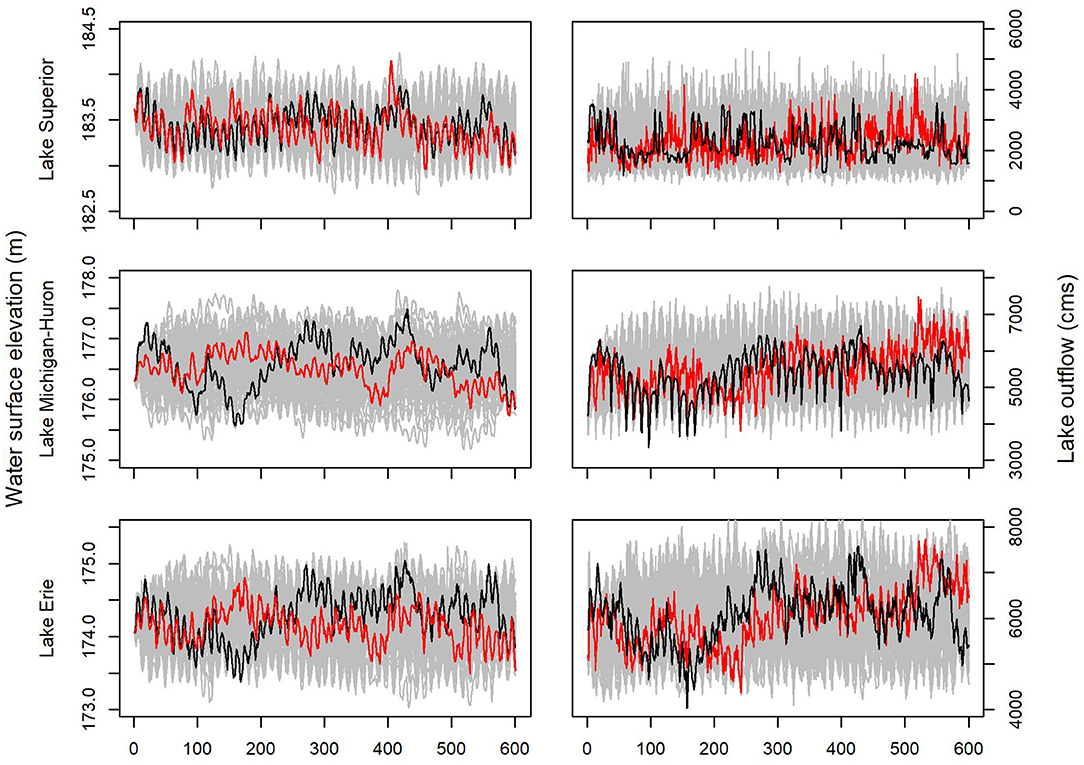
Figure 1. Comparison between simulated and observed historical time series of water levels (left) and lake outflows (right) for Lakes Superior (top), Michigan-Huron (middle), and Erie (bottom) from January 1951 through December 2000. Gray lines represent 100 ensemble members from our model simulation (randomly sampled from 1,000 to facilitate reproducibility and clarity). Black lines represent observed values, and red lines represent a single ensemble member (same member for all panels) to reflect individual simulation variability.
3.1.3. Water Level Change Analysis
Mean water levels for observed data, our historical model run, and two future water supply scenarios are summarized in Table 1.
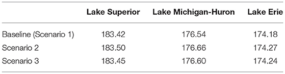
Table 1. Comparison of long-term average water levels (in meters) for each lake based on a historical simulation of the observed data period, and two future climate change scenarios.
Scenarios SC2 and SC3 indicate a slight net increase in average water level on Lake Superior, with increases of 8 cm (SC2) and 3 cm (SC3), respectively. Similar changes are expected on Lake Michigan-Huron (increases of 12 and 6 cm for SC2 and SC3, respectively) and on Lake Erie (increases of 9 and 6 cm for SC2 and SC3, respectively). Importantly, both future scenarios suggest an increase in long-term average water levels across all of the Great Lakes. These findings are consistent with the RCM-CNRM mid-century water level projections in Notaro et al. (2015) and are a plausible consequence of slight to moderate NBS increases projected by Mailhot et al. (2019) and Music et al. (2015).
All three of our model runs yield comparable marginal distributions for mean water level, as shown in Figure 2. Overlapping distributions between the baseline simulation and future scenarios indicate that any individual model run (i.e., ensemble member) may fall within the range of simulated historical values and, in some cases, even indicate a decline in water levels. Therefore, our findings indicate that while an increase in water levels is likely across the Great Lakes, our range of plausible water supply scenarios includes both the possibility of a rise or fall in long-term water levels. We notably find that continuation of observational trends in NBS components alone, via scenario SC2, results in greater water level rise than is demonstrated when RCM-based NBS component projections are incorporated via scenario SC3.
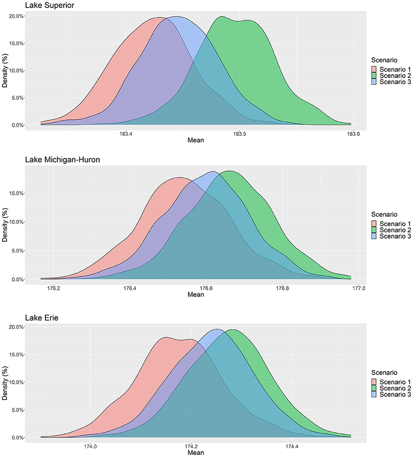
Figure 2. Probability distribution of all (600) simulated water level sequences for SC1 (red), SC2 (green), and SC3 (blue) for Lakes Superior (top), Michigan-Huron (middle), and Erie (bottom).
The seasonality of annual water level highs and lows is included in Figure 3. Scenario SC2 causes only slight shifts in the timing of annual maximum and minimum water levels, with changes of <1 week across all lakes. Peak water levels occurred an average of 3 days earlier on Lake Superior and Michigan-Huron relative to the baseline simulation, while water levels on Lake Erie peaked an average of 7 days later. The average date of annual minimum water levels did not change significantly for any lake under scenario SC2. In contrast, scenario SC3 results in a more significant shift in the seasonality of water levels across all three lakes. Water levels peak an average of 14 and 24 days sooner on Lake Superior, and Michigan-Huron, respectively, while Lake Erie remains unchanged. Lake Michigan-Huron displays the greatest shift in timing of the annual low water level, with this trough occurring an average of 11 days earlier under scenario SC3 than baseline simulations indicate.
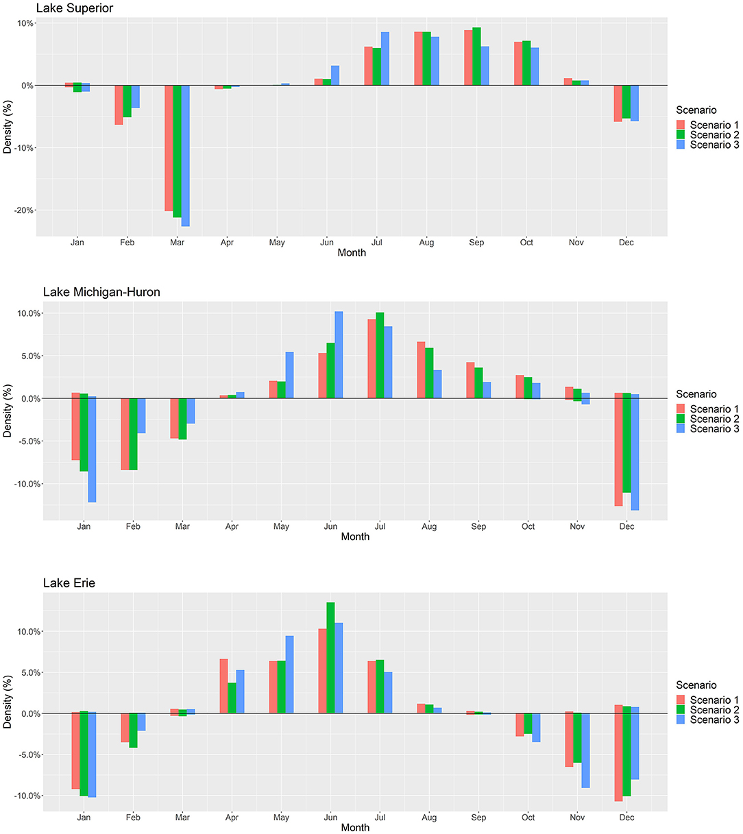
Figure 3. Frequency of occurrences of annual water level maximums (above the x-axis) and minimums (below the x-axis) for SC1 (red), SC2 (green), and SC3 (blue) for Lakes Superior (top), Michigan-Huron (middle), and Erie (bottom).
While experiencing an insignificant shift in overall timing, Lake Superior does undergo an intensification of annual lows that occur during the month of March, indicating that a temporal concentration of this seasonal inflection point may occur. Our findings are consistent with both observational trends and climate projections that annual water level rises and falls are occurring earlier, particularly annual maximum levels on Lake Superior (Lenters, 2001; Gronewold and Stow, 2014a). However, we find this shift in water level seasonality to be significantly greater in annual maximums than in annual minimums. The most apparent plausible change in the seasonal cycle of water levels is a shift earlier in the year, while there is relatively little compelling evidence for amplification or dampening effects.
Figure 4 displays the zero-centered probability density function of water levels for each simulation. While all three model simulations yield similar water level distributions, differences are evident in the tails of the distributions, representing a change in the occurrence of extreme water levels. Two standard deviations from the zero-centered mean of the historical simulation on each lake is used as a threshold to measure the frequency of extreme values. This results in a threshold of 0.3, 0.47, and 0.45 m deviations from the mean for Lake Superior, Michigan-Huron, and Erie, respectively. Water levels fall outside of these thresholds an average of 3.0% more frequently across lakes under scenario SC2 than is historically simulated, while frequency increases by an average of 2.1% under scenario SC3. Our findings also demonstrate that the increased frequency of extreme water levels is of comparable magnitude at both the high and low ends of the distribution, and that water levels are less concentrated around the mean under both scenarios. This indicates that future water levels may demonstrate greater dispersion from the mean in both directions relative to the historical record, supporting ongoing speculation about future increased variability of Great Lakes water levels (Gronewold and Rood, 2019). Increased dispersion of water levels is also consistent with the possibility of an enhancement in the annual cycle of water supply (Manabe et al., 2004; Mailhot et al., 2019), though we do not find compelling evidence of an overall amplification of seasonal water level dynamics in this study. Increasing magnitudes of both precipitation and evaporation provide another plausible explanation for greater water level variability, as imbalances in these competing hydrologic forces can result in significant water level deviations from the long-term average (Gronewold et al., 2021).
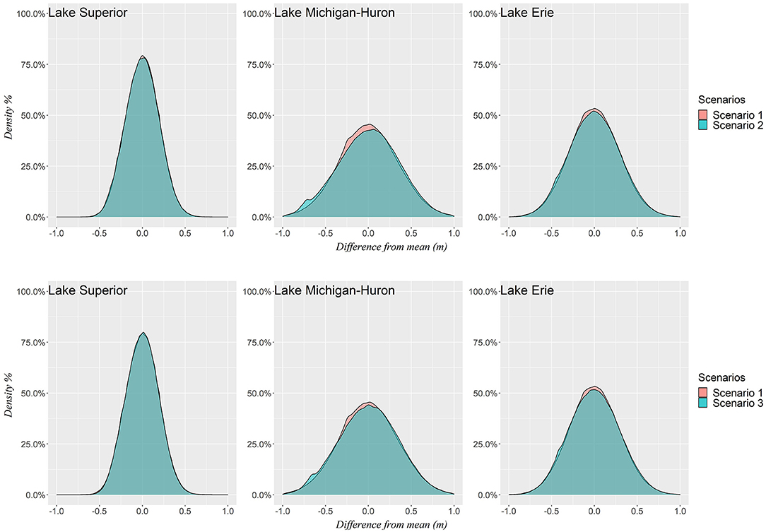
Figure 4. Comparison of zero-centered probability distributions of all simulated water levels between SC1 and SC2 (top) and SC1 and SC3 (bottom) for Lakes Superior, Michigan-Huron, and Erie.
4. Concluding Remarks
Great Lakes hydroclimate studies prior to 2011 widely used the “change-factor” method and consistently simulated significant declines in future water levels (Croley, 1990; Hartmann, 1990; Angel and Kunkel, 2010; Hayhoe et al., 2010). These findings led to a regional narrative reflecting a future of drought, aridity, and chronic low water levels (Gronewold and Stow, 2014b). The low water levels in many of these simulations, however, was a consequence of misguided modeling assumptions based on the use of air temperature as a proxy for solar radiation (Lofgren et al., 2013). A response to this narrative was catalyzed through a shift to the use of state-of-the-art downscaled RCM outputs to drive NBS and water level simulations. We have built upon this body of research by using a statistical model that maintains spatial and temporal correlation among water balance components, while allowing manipulation of the water balance component marginal distributions to reflect plausible climate change scenarios. Our results indicate that this approach (based primarily on the use of copulas) presents a promising alternative to regional water supply forecasting.
Our results indicate a slight to moderate increase in average water levels on all lakes under both plausible water supply scenarios. SC2 demonstrates greater increases than SC3, indicating that current trends in NBS components alone, if continued, could result in greater water level rise than would occur if RCM-predicted climate trends also take place. In contrast, SC3 results in greater shifts in the timing of the annual water level cycle, most notably demonstrated by the annual maximum occurring earlier in the year on Lake Superior and Michigan-Huron. Both plausible future water supply scenarios indicate an increased dispersion of water levels from the long term average. This finding indicates that, despite a rise in average levels, extreme low water levels are still likely to occur in the future.
Data Availability Statement
The raw data supporting the conclusions of this article will be made available by the authors, without undue reservation.
Author Contributions
AV contributed text and conceptualization of the study along with VL. VL encoded the copula model and ran the simulations. JJ also encoded preliminary versions of the copula and contributed text. AG oversaw all aspects of the manuscript preparation and contributed text. All authors contributed to the article and approved the submitted version.
Funding
This work was funded by the University of Michigan through the University of Michigan Undergraduate Research Opportunity Program (UROP).
Conflict of Interest
The authors declare that the research was conducted in the absence of any commercial or financial relationships that could be construed as a potential conflict of interest.
Publisher's Note
All claims expressed in this article are solely those of the authors and do not necessarily represent those of their affiliated organizations, or those of the publisher, the editors and the reviewers. Any product that may be evaluated in this article, or claim that may be made by its manufacturer, is not guaranteed or endorsed by the publisher.
Acknowledgments
The authors would like to thank Jenna Sherwin for her contributions to encoding preliminary versions of the NBS copula model, Jim Crooks for his review of model code, Ryan Armbrustmacher for his helpful input on outflow modeling and diversions, and Scott Steinschneider for his early feedback on model development.
Supplementary Material
The Supplementary Material for this article can be found online at: https://www.frontiersin.org/articles/10.3389/frwa.2022.805143/full#supplementary-material
References
Angel, J. R., and Kunkel, K. E. (2010). The response of Great Lakes water levels to future climate scenarios with an emphasis on Lake Michigan-Huron. J. Great Lakes Res. 36, 51–58. doi: 10.1016/j.jglr.2009.09.006
Apps, D., Fry, L. M., and Gronewold, A. D. (2020). Operational seasonal water supply and water level forecasting for the Laurentian Great Lakes. J. Water Resour. Plann. Manage. 146:04020072. doi: 10.1061/(ASCE)WR.1943-5452.0001214
Banda, V. D., Dzwairo, R. B., Singh, S. K., and Kanyerere, T. (2021). Trend analysis of selected hydro-meteorological variables for the Rietspruit sub-basin, South Africa. J. Water Clim. Change 12, 3099–3123. doi: 10.2166/wcc.2021.260
Bartolai, A. M., He, L., Hurst, A. E., Mortsch, L. D., Paehlke, R., and Scavia, D. (2015). Climate change as a driver of change in the Great Lakes St. Lawrence River basin. J. Great Lakes Res. 41, 45–58. doi: 10.1016/j.jglr.2014.11.012
Briley, L. J., Rood, R. B., and Notaro, M. (2021). Large lakes in climate models: A Great Lakes case study on the usability of CMIP5. J. Great Lakes Res. 47, 405–418. doi: 10.1016/j.jglr.2021.01.010
Brunk, I. W. (1968). Evaluation of channel changes in St. Clair and Detroit Rivers. Water Resour. Res. 4, 1335–1346. doi: 10.1029/WR004i006p01335
Bryan, A. M., Steiner, A. L., and Posselt, D. J. (2015). Regional modeling of surface-atmosphere interactions and their impact on Great Lakes hydroclimate. J. Geophys. Res. Atmos. 120, 1044–1064. doi: 10.1002/2014JD022316
Chen, Z., and Grasby, S. E. (2009). Impact of decadal and century-scale oscillations on hydroclimate trend analyses. J. Hydrol. 365, 122–133. doi: 10.1016/j.jhydrol.2008.11.031
Cook, R. D., and Weisberg, S. B. (1983). Diagnostics for heteroscedasticity in regrsesion. Biometrika 70, 1–10. doi: 10.1093/biomet/70.1.1
Croley, T. E. II. (1990). Laurentian Great Lakes double-CO2 climate change hydrological impacts. Clim. Change 17, 27–47. doi: 10.1007/BF00148999
Cvetkovic, M., and Chow-Fraser, P. (2011). Use of ecological indicators to assess the quality of Great Lakes coastal wetlands. Ecol. Indic. 11, 1609–1622. doi: 10.1016/j.ecolind.2011.04.005
Daba, M. H., Ayele, G. T., and You, S. (2020). Long-term homogeneity and trends of hydroclimatic variables in upper awash River Basin, Ethiopia. Adv. Meteorol. 2020, e8861959. doi: 10.1155/2020/8861959
Derecki, J. A., and Quinn, F. H. (1986). Record St. Clair River ice jam of 1984. J. Hydraul. Eng. 112, 1182–1193. doi: 10.1061/(ASCE)0733-9429(1986)112:12(1182)
Do, H. X., Mei, Y., and Gronewold, A. D. (2020a). To what extent are changes in flood magnitude related to changes in precipitation extremes? Geophys. Res. Lett. 47, e2020Gl088684. doi: 10.1029/2020GL088684
Do, H. X., Smith, J. P., Fry, L. M., and Gronewold, A. D. (2020b). Seventy-year long record of monthly water balance estimates for Earth's largest lake system. Sci. Data 7, 276. doi: 10.1038/s41597-020-00613-z
Frigon, A., Music, B., and Slivitzky, M. (2010). Sensitivity of runoff and projected changes in runoff over Quebec to the update interval of lateral boundary conditions in the Canadian RCM. Meteorol. Zeitsch. 19, 225. doi: 10.1127/0941-2948/2010/0453
Fujisaki-Manome, A., Fitzpatrick, L., Gronewold, A. D., Anderson, E. J., Lofgren, B. M., Spence, C., et al. (2017). Turbulent heat fluxes during an extreme lake effect snow event. J. Hydrometeorol. 18, 3145–3163. doi: 10.1175/JHM-D-17-0062.1
Gelman, A. J., Carlin, J. B., Stern, H. S., and Rubin, D. B. (2004). Bayesian Data Analysis. Boca Raton, FL: Chapman & Hall; CRC Press. doi: 10.1201/9780429258480
Gessler, D., Gessler, J., and Watson, C. C. (1998). Prediction of discontinuity in stage-discharge rating curves. J. Hydraul. Eng. 124, 243–252. doi: 10.1061/(ASCE)0733-9429(1998)124:3(243)
Ghanbari, R. N., and Bravo, H. R. (2008). Coherence between atmospheric teleconnections, Great Lakes water levels, and regional climate. Adv. Water Resour. 31, 1284–1298. doi: 10.1016/j.advwatres.2008.05.002
Gronewold, A. D., Bruxer, J., Durnford, D., Smith, J. P., Clites, A. H., Seglenieks, F., et al. (2016). Hydrological drivers of record-setting water level rise on Earth's largest lake system. Water Resour. Res. 52, 4026–4042. doi: 10.1002/2015WR018209
Gronewold, A. D., Clites, A. H., Hunter, T. S., and Stow, C. A. (2011). An appraisal of the Great Lakes advanced hydrologic prediction system. J. Great Lakes Res. 37, 577–583. doi: 10.1016/j.jglr.2011.06.010
Gronewold, A. D., Clites, A. H., Smith, J. P., and Hunter, T. S. (2013a). A dynamic graphical interface for visualizing projected, measured, and reconstructed surface water elevations on the earth's largest lakes. Environ. Model. Softw. 49, 34–39. doi: 10.1016/j.envsoft.2013.07.003
Gronewold, A. D., Do, H. X., Mei, Y., and Stow, C. A. (2021). A tug-of-war within the hydrologic cycle of a continental freshwater basin. Geophys. Res. Lett. 48, e2020GL090374. doi: 10.1029/2020GL090374
Gronewold, A. D., Fortin, V., Caldwell, R., and Noel, J. (2018). Resolving hydrometeorological data discontinuities along an international border. Bull. Am. Meteorol. Soc. 99, 899–910. doi: 10.1175/BAMS-D-16-0060.1
Gronewold, A. D., Fortin, V., Lofgren, B. M., Clites, A. H., Stow, C. A., and Quinn, F. H. (2013b). Coasts, water levels, and climate change: a Great Lakes perspective. Clim. Change 120, 697–711. doi: 10.1007/s10584-013-0840-2
Gronewold, A. D., and Rood, R. B. (2019). Recent water level changes across Earth's largest lake system and implications for future variability. J. Great Lakes Res. 45, 1–3. doi: 10.1016/j.jglr.2018.10.012
Gronewold, A. D., Smith, J. P., Read, L. K., and Crooks, J. L. (2020). Reconciling the water balance of large lake systems. Adv. Water Resour. 137, 103505. doi: 10.1016/j.advwatres.2020.103505
Gronewold, A. D., and Stow, C. A. (2014a). Unprecedented seasonal water level dynamics on one of the Earth's largest lakes. Bull. Am. Meteorol. Soc. 95, 15–17. doi: 10.1175/BAMS-D-12-00194.1
Gronewold, A. D., and Stow, C. A. (2014b). Water loss from the Great Lakes. Science 343, 1084–1085. doi: 10.1126/science.1249978
Gronewold, A. D., Stow, C. A., Vijayavel, K., Moynihan, M. A., and Kashian, D. R. (2013c). Differentiating Enterococcus concentration spatial, temporal, and analytical variability in recreational waters. Water Res. 47, 2141–2152. doi: 10.1016/j.watres.2012.12.030
Gula, J., and Peltier, W. R. (2012). Dynamical downscaling over the Great Lakes Basin of North America using the WRF regional climate model: the impact of the Great Lakes system on regional greenhouse warming. J. Clim. 25, 7723–7742. doi: 10.1175/JCLI-D-11-00388.1
Gyamfi, C., Ndambuki, J. M., and Salim, R. W. (2016). A Historical analysis of rainfall trend in the olifants basin in South Africa. Earth Sci. Res. 5, 129. doi: 10.5539/esr.v5n1p129
Hartmann, H. C. (1990). Climate change impacts on Laurentian Great Lakes levels. Clim. Change 17, 49–67. doi: 10.1007/BF00149000
Hayhoe, K., VanDorn, J., Croley II, T. E., Schlegal, N., and Wuebbles, D. (2010). Regional climate change projections for Chicago and the US Great Lakes. J. Great Lakes Res. 36, 7–21. doi: 10.1016/j.jglr.2010.03.012
Hu, M., Sayama, T., Try, S., Takara, K., and Tanaka, K. (2019). Trend analysis of hydroclimatic variables in the Kamo River Basin, Japan. Water 11, 1782. doi: 10.3390/w11091782
Hunter, T. S., Clites, A. H., Campbell, K. B., and Gronewold, A. D. (2015). Development and application of a monthly hydrometeorological database for the North American Great Lakes - Part I: precipitation, evaporation, runoff, and air temperature. J. Great Lakes Res. 41, 65–77. doi: 10.1016/j.jglr.2014.12.006
Labuhn, K., Gronewold, A. D., Calappi, T. J., MacNeil, A., Brown, C., and Anderson, E. J. (2020). Towards an operational flow forecasting system for the Upper Niagara River. J. Hydraul. Eng. 146, 05020006. doi: 10.1061/(ASCE)HY.1943-7900.0001781
Latif, S., and Mustafa, F. (2020). Parametric vine copula construction for flood analysis for Kelantan River Basin in Malaysia. Civil Eng. J. 6, 1470–1491. doi: 10.28991/cej-2020-03091561
Laux, P., Vogl, S., Qiu, W., Knoche, H. R., and Kunstmann, H. (2011). Copula-based statistical refinement of precipitation in RCM simulations over complex terrain. Hydrol. Earth Syst. Sci. 15, 2401–2419. doi: 10.5194/hess-15-2401-2011
Lee, T., and Salas, J. D. (2011). Copula-based stochastic simulation of hydrological data applied to Nile River flows. Hydrol. Res. 42, 318–330. doi: 10.2166/nh.2011.085
Lenters, J. D. (2001). Long-term trends in the seasonal cycle of Great Lakes water levels. J. Great Lakes Res. 27, 342–353. doi: 10.1016/S0380-1330(01)70650-8
Lofgren, B. M. (2004). A model for simulation of the climate and hydrology of the Great Lakes basin. J. Geophys. Res. 109, D18. doi: 10.1029/2004JD004602
Lofgren, B. M., and Gronewold, A. D. (2013). Reconciling alternative approaches to projecting hydrologic impacts of climate change. Bull. Am. Meteorol. Soc. 94, ES133–ES135. doi: 10.1175/BAMS-D-13-00037.1
Lofgren, B. M., Gronewold, A. D., Acciaioli, A., Cherry, J., Steiner, A. L., and Watkins, D. W. (2013). Methodological approaches to projecting the hydrologic impacts of climate change. Earth Interact. 17, 1–19. doi: 10.1175/2013EI000532.1
Lofgren, B. M., Hunter, T. S., and Wilbarger, J. (2011). Effects of using air temperature as a proxy for potential evapotranspiration in climate change scenarios of Great Lakes basin hydrology. J. Great Lakes Res. 37, 744–752. doi: 10.1016/j.jglr.2011.09.006
Lofgren, B. M., and Rouhana, J. (2016). Physically plausible methods for projecting changes in Great Lakes water levels under climate change scenarios. J. Hydrometeorol. 17, 2209–2223. doi: 10.1175/JHM-D-15-0220.1
Lu, S., Shen, H. T., and Crissman, R. D. (1999). Numerical study of ice jam dynamics in upper Niagara River. J. Cold Reg. Eng. 13, 78–102. doi: 10.1061/(ASCE)0887-381X(1999)13:2(78)
MacKay, M., and Seglenieks, F. (2013). On the simulation of Laurentian Great Lakes water levels under projections of global climate change. Clim. Change 117, 55–67. doi: 10.1007/s10584-012-0560-z
Mailhot, E., Music, B., Nadeau, D. F., Frigon, A., and Turcotte, R. (2019). Assessment of the Laurentian Great Lakes' hydrological conditions in a changing climate. Clim. Change 157, 243–259. doi: 10.1007/s10584-019-02530-6
Maity, R. (2018). “Theory of copula in hydrology and hydroclimatology,” in Statistical Methods in Hydrology and Hydroclimatology (Singapore: Springer), 381–424. doi: 10.1007/978-981-10-8779-0_10
Manabe, S., Wetherald, R. T., Milly, P. C., Delworth, T. L., and Stouffer, R. J. (2004). Century-scale change in water availability: CO2 - quadrupling experiment. Clim. Change 64, 59–76. doi: 10.1023/B:CLIM.0000024674.37725.ca
Marchand, D., Sanderson, M., Howe, D., and Alpaugh, C. (1988). Climatic change and Great Lakes levels: the impact on shipping. Clim. Change 12, 107–133. doi: 10.1007/BF00138935
Meyer, E. S., Characklis, G. W., Brown, C., and Moody, P. (2016). Hedging the financial risk from water scarcity for Great Lakes shipping. Water Resour. Res. 52, 227–245. doi: 10.1002/2015WR017855
Miller, W. P., and Piechota, T. C. (2008). Regional analysis of trend and step changes observed in hydroclimatic variables around the Colorado River Basin. J. Hydrometeorol. 9, 1020–1034. doi: 10.1175/2008JHM988.1
Millerd, F. (2011). The potential impact of climate change on Great Lakes international shipping. Clim. Change 104, 629–652. doi: 10.1007/s10584-010-9872-z
Milly, P. C., and Dunne, K. A. (2017). A hydrologic drying bias in water-resource impact analyses of anthropogenic climate change. J. Am. Water Resour. Assoc. 53, 822–838. doi: 10.1111/1752-1688.12538
Mortsch, L. D., and Quinn, F. H. (1996). Climate change scenarios for Great Lakes Basin ecosystem studies. Limnol. Oceanogr. 41, 903–911. doi: 10.4319/lo.1996.41.5.0903
Moukomla, S., and Blanken, P. (2016). Remote sensing of the North American Laurentian Great Lakes' surface temperature. Remote Sensing 8, 286. doi: 10.3390/rs8040286
Music, B., Frigon, A., Lofgren, B., Turcotte, R., and Cyr, J.-F. (2015). Present and future Laurentian Great Lakes hydroclimatic conditions as simulated by regional climate models with an emphasis on Lake Michigan-Huron. Clim. Change 130, 603–618. doi: 10.1007/s10584-015-1348-8
Nagler, T., Schepsmeier, U., Stoeber, J., Brechmann, E. C., Graeler, B., and Erhardt, T. (2021). VineCopula: Statistical Inference of Vine Copulas. Technical report.
Nevers, M. B., and Whitman, R. L. (2011). Efficacy of monitoring and empirical predictive modeling at improving public health protection at Chicago beaches. Water Res. 45, 1659–1668. doi: 10.1016/j.watres.2010.12.010
Noguchi, K., Gel, Y. R., and Duguay, C. R. (2011). Bootstrap-based tests for trends in hydrological time series, with application to ice phenology data. J. Hydrol. 410, 150–161. doi: 10.1016/j.jhydrol.2011.09.008
Notaro, M., Bennington, V., and Lofgren, B. M. (2015). Dynamical downscaling-based projections of Great Lakes water levels. J. Climate 28, 9721–9745. doi: 10.1175/JCLI-D-14-00847.1
Notaro, M., Holman, K. D., Zarrin, A., Fluck, E., Vavrus, S. J., and Bennington, V. (2013). Influence of the Laurentian Great Lakes on regional climate. J. Climate 26, 789–804. doi: 10.1175/JCLI-D-12-00140.1
Pouliasis, G., Torres-Alves, G. A., and Morales-Napoles, O. (2021). Stochastic modeling of hydroclimatic processes using vine copulas. Water 13, 2156. doi: 10.3390/w13162156
Press, S. J. (2003). Subjective and Objective Bayesian Statistics: Principles, Models, and Applications. Hoboken, NJ: Wiley-Interscience.
Pryor, S. C., Scavia, D., Downer, C., Gaden, M., Iverson, L., Nordstrom, R., et al. (2014). “Midwest climate change impacts in the United States: The third national climate assessment,” in National Climate Assessment Report, eds J. M. Melillo, T. C. Richmond, and G. W. Yohe (Washington, DC: US Global Change Research Program), 418–440.
Quinn, F. H. (1978). Hydrologic response model of the North American Great Lakes. J. Hydrol. 37, 295–307. doi: 10.1016/0022-1694(78)90021-5
Quinn, F. H. (2002). Secular changes in Great Lakes water level seasonal cycles. J. Great Lakes Res. 28, 451–465. doi: 10.1016/S0380-1330(02)70597-2
Quinn, F. H., Clites, A. H., and Gronewold, A. D. (2020). Evaluating estimates of channel flow in a continental-scale lake-dominated basin. J. Hydrol. Eng. 146:05019008. doi: 10.1061/(ASCE)HY.1943-7900.0001685
Quinn, F. H., and Edstrom, J. (2000). Great Lakes diversions and other removals. Can. Water Resour. J. 25, 125–151. doi: 10.4296/cwrj2502125
Schmidt, A. R., and Yen, B. C. (2008). Theoretical development of stage-discharge ratings for subcritical open-channel flows. J. Hydraul. Eng. 134, 1245–1256. doi: 10.1061/(ASCE)0733-9429(2008)134:9(1245)
Schölzel, C., and Friederichs, P. (2008). Multivariate non-normally distributed random variables in climate research - introduction to the copula approach. Nonlin. Process. Geophys. 15, 761–772. doi: 10.5194/npg-15-761-2008
Sen, P. K. (1968). Estimates of the regression coefficient based on Kendall's Tau. J. Am. Stat. Assoc. 63, 1379–1389. doi: 10.1080/01621459.1968.10480934
Smith, J. P., Hunter, T. S., Clites, A. H., Stow, C. A., Slawecki, T., Muhr, G. C., et al. (2016). An expandable web-based platform for visually analyzing basin-scale hydro-climate time series data. Environ. Model. Softw. 78, 97–105. doi: 10.1016/j.envsoft.2015.12.005
Thompson, A. F., Rodrigues, S. N., Fooks, J. C., Oberg, K. A., and Calappi, T. J. (2020). Comparing discharge computation methods in Great Lakes connecting channels. J. Hydrol. Eng. 25:05020007. doi: 10.1061/(ASCE)HE.1943-5584.0001904
Trenberth, K. E. (1997). The definition of El Ni no. Bull. Am. Meteorol. Soc. 78, 2771–2777. doi: 10.1175/1520-0477(1997)078<2771:TDOENO>2.0.CO;2
Van Vuuren, D. P., Edmonds, J., Kainuma, M., Riahi, K., Thomson, A., Hibbard, K., et al. (2011). The representative concentration pathways: an overview. Clim. Change 109, 5–31. doi: 10.1007/s10584-011-0148-z
Wang, F., Shao, W., Yu, H., Kan, G., He, X., Zhang, D., et al. (2020). Re-evaluation of the power of the Mann-Kendall test for detecting monotonic trends in hydrometeorological time series. Front. Earth Sci. 8, 14. doi: 10.3389/feart.2020.00014
Westerberg, I., Guerrero, J. L., Seibert, J., Beven, K. J., and Halldin, S. (2011). Stage-discharge uncertainty derived with a non-stationary rating curve in the Choluteca River, Honduras. Hydrol. Process. 25, 603–613. doi: 10.1002/hyp.7848
Winkler, J. A. (2015). Selection of climate information for regional climate change assessments using regionalization techniques: an example for the Upper Great Lakes Region, USA. Int. J. Climatol. 35, 1027–1040. doi: 10.1002/joc.4036
Wright, D. M., Posselt, D. J., and Steiner, A. L. (2013). Sensitivity of lake-effect snowfall to lake ice cover and temperature in the Great Lakes region. Month. Weath. Rev. 141, 670–689. doi: 10.1175/MWR-D-12-00038.1
Keywords: climate change, statistical model, Great Lakes, water supplies, copula
Citation: VanDeWeghe A, Lin V, Jayaram J and Gronewold AD (2022) Changes in Large Lake Water Level Dynamics in Response to Climate Change. Front. Water 4:805143. doi: 10.3389/frwa.2022.805143
Received: 29 October 2021; Accepted: 03 February 2022;
Published: 13 April 2022.
Edited by:
Julie A. Winkler, Michigan State University, United StatesReviewed by:
Simon Papalexiou, University of Saskatchewan, CanadaJim Angel, University of Illinois at Urbana-Champaign, United States
Copyright © 2022 VanDeWeghe, Lin, Jayaram and Gronewold. This is an open-access article distributed under the terms of the Creative Commons Attribution License (CC BY). The use, distribution or reproduction in other forums is permitted, provided the original author(s) and the copyright owner(s) are credited and that the original publication in this journal is cited, in accordance with accepted academic practice. No use, distribution or reproduction is permitted which does not comply with these terms.
*Correspondence: Andrew D. Gronewold, ZHJld2dyb25AdW1pY2guZWR1