Training a hidden Markov model with PMDI and temperature to create climate informed scenarios

Tezcan, Burcu; Garcia, Margaret

doi:10.3389/frwa.2025.1472695

ORIGINAL RESEARCH article

Front. Water, 13 June 2025

Sec. Water and Hydrocomplexity

Volume 7 - 2025 | https://doi.org/10.3389/frwa.2025.1472695

This article is part of the Research TopicAdapting Water Management to Climate Change: Challenges for Vulnerable Regions and Extreme EventsView all 3 articles

Training a hidden Markov model with PMDI and temperature to create climate informed scenarios

Burcu Tezcan^*

Margaret Garcia

School of Sustainable Engineering and the Built Environment, Arizona State University, Tempe, AZ, United States

Understanding the nature of climatic change impacts on spatial and temporal hydroclimatic patterns is important to the development of timely and spatially explicit adaptation options. However, regime-switching behavior of hydroclimatic variables complicates the modelling process as many traditional time series methods do not capture this behavior. Accurately representing spatial correlation across hydroclimatic regimes is particularly important for water resources planning in large watersheds such as the Colorado River, and regions where interbasin transfers and shared demand nodes link multiple watersheds. Here, we developed a hidden Markov model (HMM) with covariates that generates an ensemble of plausible future regional scenarios of the Palmer modified drought index (PMDI) for any projected temperature sequence. The resulting spatially explicit scenarios represent the historical spatial and temporal patterns of the training data while incorporating non-stationarity by conditioning on temperature. These ensembles can aid water resources managers, infrastructure planners, and government policymakers tasked with building of more resilient water systems. Moreover, these ensembles can be used to generate streamflow ensembles, which, in turn, will be a valuable input to study the impact of climate change on regional hydrology.

1 Introduction

Over the last century interbasin water transfers have fulfilled growing demands and facilitated economic growth (Siddik et al., 2023). Linking previously disconnected watersheds has also enabled water suppliers to increase reliability during droughts by balancing multiple supply sources. The Western United States (U.S.) is a key example of this where the Colorado River, is linked to the Rio Grande and California State Water Project via interbasin transfers and shared demand nodes (National Research Council, 2007). This network of supply systems provides a buffer for individual water suppliers in times of stress or change by enabling users to balance a portfolio of water sources (Anderies, 2015). However, gaps in our understanding of spatial correlation of wet and dry conditions across regions, such as the Western U.S., limit our ability to fully characterize the reliability of these systems.

At the regional scale hydroclimatic variables exhibit regimes or recurrent, large scale spatial patterns in one or more hydroclimatic variables. The regime-shifting (e.g., the transition between different regimes) behavior of hydroclimate patterns, influenced by large-scale climatic factors such as El Niño, the Pacific Decadal Oscillation, and the Multi-Decadal Oscillation presents an additional challenge (Cayan, 1996; Ho et al., 2018). These climatic patterns interact to shape hydroclimatic regimes, yet their effects cannot be resolved into a clean variable set (Ho et al., 2018). Hydroclimatic regimes often lead to prolonged periods of high or low water availability, making water management and planning even more complicated (Bracken et al., 2014). However, the ability of large-scale climate factors to explain regional regime-shifting behavior of hydroclimate patterns is limited since hydroclimatic regimes can also be influenced by regional phenomena (Gupta et al., 2023a; Dettinger and Cayan, 2014). Furthermore, hydrological systems are non-stationary (Zhao et al., 2018; Milly et al., 2008) with observed and projected changes in the intensity, duration, and frequency of hydrological extremes (Marvel et al., 2023; Jakob, 2013). The formulation of effective regional water management strategies requires an understanding of spatio-temporal patterns, including regime-shifts, and how these patterns may change in the future.

A variety of statistical methods have been applied to the regionalization of hydrological variables such as regression analysis (Merz and Blöschl, 2004), proximity-based methods (Betterle et al., 2019), geostatistical techniques (e.g., inverse distances, kriging, space–time models) (Adamowski and Bocci, 2001; Bourges et al., 2012), machine learning algorithms (Song et al., 2022; Wang et al., 2023), and combination of time series and spatial statistical methods (Adamowski et al., 2013). Despite the flexibility of statistical methods, they are limited by computational requirements and data availability (Blöschl et al., 2013a). Physically-based classification frameworks also have been used to characterize regional hydrological variables (Doulatyari et al., 2017), yet these too are limited by the availability of observational data.

Building this understanding necessitates quantification of regional spatiotemporal patterns from field measurements, which is challenged by limited observational data (Betterle et al., 2017; Blöschl et al., 2013b; Razavi and Coulibaly, 2013; Sivapalan et al., 2003). The relatively short duration of observational data limits the ability to characterize possible nonstationarity, and regime switching behavior of hydroclimate patterns, particularly when regime lengths extend over a decade or more (Wilhelm et al., 2018). Several studies concluded that developing a reliable model using long time series—spanning at least more than 100 years—that cover a broad range of hydrological variability, from yearly to multidecadal variations, is required to identify persistence structure of hydroclimate patterns, capture non-stationarity, and feed into projections (Thyer et al., 2006; Thyer and Kuczera, 2000; Nasri et al., 2020; Gupta et al., 2023b). Such long time series thereby opens new opportunities to understand regional hydrological patterns to inform decision making, policy, and management practices for networked river systems.

Generating future scenarios that account for climate change is critical for water management but there are difficulties in projecting spatial patterns of hydrological variables across multiple sites using the general circulation models (GCMs) (Vallam and Qin, 2017), as projections are coarse and unsuitable for regional studies (Fowler et al., 2007; Xu, 1999). While the recent generation of models in Coupled Model Intercomparison Project Phase 6 (CMIP6) offers improved resolutions (Liang-Liang et al., 2022), GCMs may still remain inadequate for providing the detailed regional information required for climate change impact studies including hydrological studies at river basin scale (Banda et al., 2022). To overcome this challenge, statistical downscaling methods, including regression modeling, weather generators, and weather typing schemes, machine learning models have been employed to provide finer-resolution data for climate change impact assessments (Vrac and Naveau, 2007; Shen et al., 2018; Guo et al., 2019; Prathom and Champrasert, 2023; Gu et al., 2021). Alternatively, regional climate models (RCMs) which are nested in the GCMs can be employed for deriving climatic variables for a specific region using dynamic downscaling methods which yield spatially distributed fields of climatic variables while preserving certain spatial correlations and maintaining physically realistic relationships between climatic variables (Maurer and Hidalgo, 2008). However, these methods are computationally expensive and only available for limited regions (Salehnia et al., 2019; Sunyer et al., 2012; Tisseuil et al., 2010; Xu et al., 2019). Additionally, outputs from recent GCMs have significantly improved in spatial resolution and wider applicability, closing the gap with RCMs. This advancement is contributing to a decreased reliance on RCMs for policy-making purposes (Tapiador et al., 2020). Moreover, GCMs are limited by the large uncertanities, and large discrepancies in the simulation of hyrological changes (Wu et al., 2024). For example, output of these models poorly represents regional precipitation (Rocheta et al., 2014; Lehner et al., 2020; Zhou et al., 2020; Srivastava et al., 2020), and drought persistence (Moon et al., 2018).

Stochastic modelling provides valuable tools for understanding and managing uncertainty to support decision-making (Hui et al., 2018; Ajami et al., 2008). According to Brekke et al. (2009) stochastic modeling can be useful for developing climate scenarios that include a wide range of potential hydroclimatic conditions. The expanded variability may allow more robust evaluation of planning alternatives. However, regime-switching complicates the modelling process because many traditional stochastic time series models (e.g., autoregressive-moving average) are inadequate in capturing regime-shifting characteristics, leading to a misrepresentation of the risk associated with prolonged wet and dry periods (Bracken et al., 2014). As a result, this misrepresentation can adversely affect management and planning efforts. Bracken et al. (2014) addressed this by developing a climate informed hidden Markov model (HMM) that used information from climate indices (e.g., Niño3 index) to improve the representation of temporal behavior. However, their method does not incorporate GCM outputs and therefore does not address the challenge of creating GCM informed projections. Moreover, investigating regime-switching behavior only through the context of global oscillations will result in incomplete understanding of weather regimes, as they are also influenced by regional phenomena (Gupta et al., 2023a).

Advanced stochastic techniques such as HMMs offer a flexible approach to capture the regime-switching behavior of hydroclimate patterns (Bracken et al., 2014; Ho et al., 2018). HMMs enable the conceptualization of climatic patterns as latent or hidden variables, considering their interconnected influence on hydroclimatic regimes (Ho et al., 2018). Moreover, HMMs provide more useful information to quantify spatiotemporal variabilities while considering climatic states and trends, in comparison to methods that would seek to cluster the time series or find lower dimensional patterns (e.g., wavelet analysis) (Ho et al., 2018). Thus, HMMs have been extensively used in hydroclimatic analysis including studies to quantify spatio-temporal variabilities and trends (Bracken et al., 2014, 2016; Ho et al., 2018; Holsclaw et al., 2017; Hughes and Guttorp, 1994; Prairie et al., 2008; Hernández et al., 2020; Zucchini and Guttorp, 1991), to downscale hydrological variables from GCMs (Jiang et al., 2023), to model paleoreconstruction data (Nasri et al., 2020; Gupta et al., 2023b), weather generation (Paciorek, 2022) and other hydrologic applications (Guilpart et al. 2021; Sun et al. 2023). Covariates can be incorporated into HMMs by including them to the parameters of the state dependent distributions, the transition probability matrix, or a combination of both (Zucchini et al., 2016). Such predictor variables offer one way to link the HMM, which is constructed based on past observations, to future projections.

To address data limitations, paleoreconstruction data offers a promising approach for supplementing relatively short observational records to better understand the long-term climate variability (Cook et al., 1999). These paleoreconstructions have been employed to inform water resources planning and policy especially in the areas which are prone to high levels of spatiotemporal variability or in case of modeling supply systems that span multiple river basins (Carrier et al., 2013; Rice et al., 2009; Woodhouse and Lukas, 2006a, 2006b; Gupta et al., 2023b). Paleoreconstructions of the Palmer modified drought index (PMDI) and temperature across North America are examples of such records (Cook et al., 2010; Wahl and Smerdon, 2012a, 2012b). Recent studies use a gridded paleo-proxy called the Living Blended Drought Atlas (LBDA) (Ho et al., 2018) and standardized precipitation index (SPI) (Gupta et al., 2023a) to reconstruct weather regimes, and LBDA to reconstruct streamflow across the U. S (Ho et al., 2016, 2017). Paleoreconstructions have proven valuable for understading the drought statistics, as well as assesing the probability of co-occurance of wet and dry periods across a regional watershed of multiple interlinked watersheds (Ravindranath et al., 2019; Nasri et al., 2020). While most hydrological data reconstructions are focused on catchment and gauge-specific applications (Bracken et al., 2016; Ravindranath et al., 2019; Woodhouse et al., 2024), limited prior research addressed inter-site and inter-basin dependencies for better water supply management of interconnected networks of watersheds for regional water supply (Littell et al., 2023). For example, Bracken et al. (2016) reconstructed flows at 20 sites in the Upper Colorado River Basin demonstrating the ability to preserve inter-site correlations and dynamic representation of uncertainty in each reconstructed year. Catchment-specific reconstructions provide valuable insights only for local water management practices, yet many catchments are still lacking spatio-temporal coverage of reconstruction of hydrologic variables (Ho et al., 2017; Littell et al., 2023). A variety of methods (e.g., hierarchical clustering method, Bayesian hierarchical non-homogenous HMM) have been used to quantify the spatiotemporal structure of paleoreconstruction data (Chen et al., 2019; Bracken et al., 2016; Carrier et al., 2013; Ho et al., 2016; Rao et al., 2018). However, the high dimensionality of paleoreconstruction data, coupled with its large scale, makes it complex to analyze and manage large datasets. Additionally, given the potential for hydrological change driven by a changing climate, an understanding of future patterns is also needed.

Previous applications demonstrate that HMM can simulate regional hydrological patterns in space and time (Guo et al., 2018; Bracken et al., 2014; Najibi et al., 2021). However, these models without covariates are trained on historic data and do not have the capacity to make projections or create scenarios to explore the future. This gap motivates the following research questions: (1) how to generate an ensemble of future regional climate informed scenarios across the Western U.S. consistent with historic spatio-temporal patterns and future temperature changes? (2) how to cope with the high dimensionality of paleoreconstruction data and thereby enable a computationally efficient model for large regions? In answering these questions, we expand upon prior work (e.g., Steinschneider et al., 2019; Ho et al., 2018) by constructing a HMM with covariates that can both characterize historical spatiotemporal patterns and make projections of PMDI informed by temperature projections. Temperature is selected as the covariates because it is both available in the paleoreconstruction record (Wahl and Smerdon, 2012a, 2012b) and a well vetted output of GCM projections (Woldemeskel et al., 2016).

While both temperature and precipitation influence PMDI, variations in precipitation exhibit significant diversity across different climate models and geographical regions (Bradford et al., 2020). For example, Srivastava et al. (2020) found that most CMIP6 models tend to overestimate both the frequency and variability of wet period durations in the Western U.S. Similarly, Kunkel et al. (2020) showed that the Western U.S. exhibits mixed trends of annual precipitation events for the observed period. This highlights the complex nature of precipitation patterns in the Western U.S., where annual precipitation trends can vary significantly depending on the period of record and spatial location. In contrast significant temperature change is detected in observations (Udall and Overpeck, 2017; Griffin and Anchukaitis, 2014; Marvel et al., 2023), is consistently projected, and is established as a significant driver of aridification in the Western U.S. (Overpeck and Udall, 2020; Williams et al., 2020). Thus, incorporating the effects of temperature change in future hydrological scenarios is critical to capture the dominant impact of climate change on hydrology in the region. We also apply principal component analysis (PCA) to address the challenges posed by the high dimensionality of paleoreconstruction data by effectively capturing its temporal and spatial dependencies, thereby mitigating the computational complexity of HMM. Further, our approach improves upon traditional time series models which are based on short-term memory and stationarity that cause a weak persistence and lower probability of long wet and dry spells due to a weak autocorrelation (Bracken et al., 2014). We address these research questions in the context of the Western U.S. The Western U.S. region is an ideal test case because of its uncertain climate variability which affects water resources planning and management.

2 Materials and methods

2.1 Study area

This study focuses on the Western U.S. watersheds, particularly the Colorado River and interconnected watersheds linked by interbasin transfers and shared demand nodes, such as Rio Grande River Basin, Central Valley Water Project, Southern California, Los Angeles Aqueduct source watersheds, Central Utah and Strawberry water project, Arkansas River, South Platte River, Little Snake River, Imperial and Coachella Valleys, and parts of Mexico (e.g., Baja California and Sonora). The interconnected nature of these watersheds motivates this investigation of regional hydroclimatic patterns, as droughts occur at larger spatiotemporal scales for the western part of U.S., typically spreading over hundreds to thousands of square kilometers. Droughts in the western and most of the central U.S. commonly originate from northwestern direction (Konapala and Mishra, 2017). Hence, the study area is defined as 30–49° N, 97.1–124.9° W (Figure 1). Spatially gridded PMDI and temperature data are extracted based on the study area boundary.

Figure 1

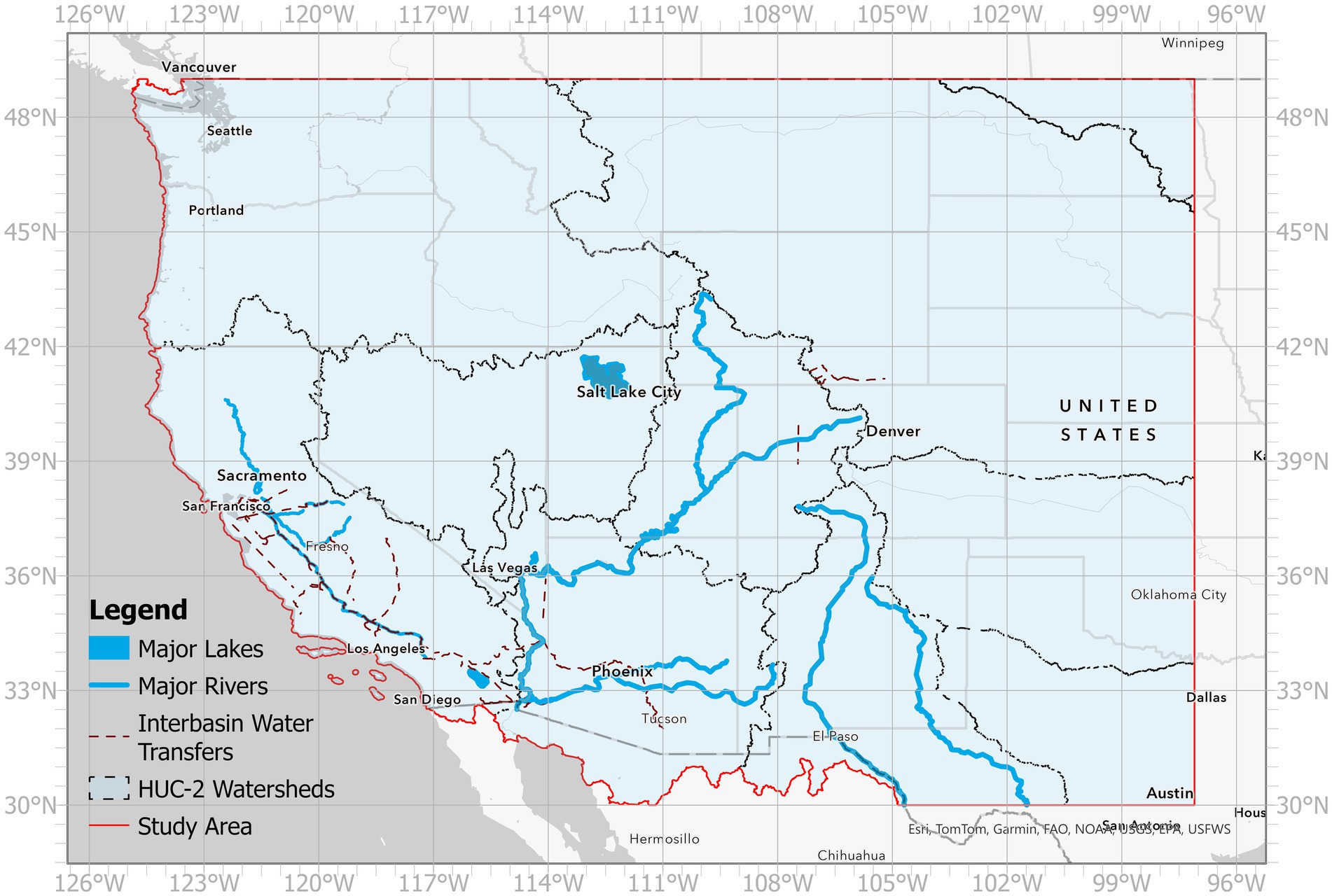
Figure 1. Map of the study area with the HUC-2 hydrologic regions (blue polygons). The study area is defined as 30–49° N, 97.1–124.9° W.

Figure 1 shows the study area along with the 11 U.S. Geological Survey (USGS) HUC-2 (2-digit hydrologic unit code) hydrologic regions.

2.2 Data

Paleo PMDI data and paleo temperature anomalies used in this study are obtained from the National Oceanic and Atmospheric Administration (NOAA) database (Cook et al., 2010; Wahl and Smerdon, 2012a, 2012b). Temperature projections are taken from the bias corrected CMIP6 climate projections with the shared socioecomic pathways (SSP) 245 scenario, which is an update to representative concentration pathway (RCP) 4.5 scenario, with an additional radiative forcing of 4.5 W/m² by the year 2100 (Xu et al., 2021). This scenario is the medium pathway of future greenhouse gas emissions and assumes that climate protection measures are being taken (Böttinger and Kasang, 2024). This scenario was selected to demonstrate the technique but any temperature projections from any scenario could be applied. Resampling is performed with bilinear technique for the reconstructed temperature anomalies and the temperature projections to match the 0.5 × 0.5 paleo PMDI data grid over the study area. The choice of study period is guided by a trade-off between data availability in terms of record length and spatial coverage. Annually resolved paleoreconstruction records and temperature projections are used to test hydroclimatic variability over time scales related to water resources management and planning. The overview of data used in this study is given in Table 1.

Table 1

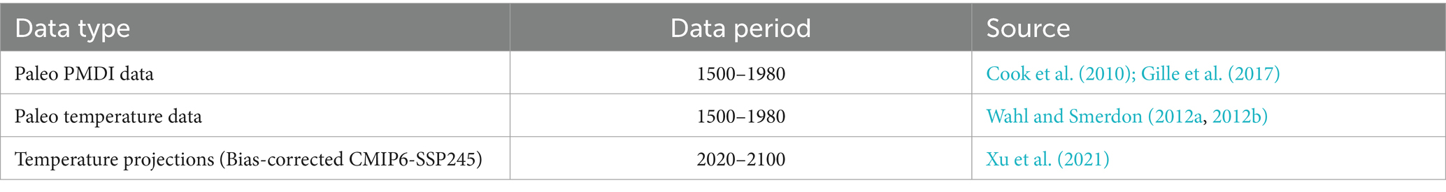
Table 1. Overview of data.

2.2.1 Living blended drought atlas

The PMDI is a modification of the Palmer drought severity index (PDSI), which uses readily available temperature and precipitation data to calculate relative dryness of a region and the severity of wet and dry events (Palmer, 1965). It can reflect the mechanism of drought and can be used to monitor long-term evolution of droughts (Yu et al., 2019). The difference between PMDI and PDSI is in the transition periods between dry and wet conditions. For the PDSI, a dry/wet index is calculated when the probability that a dry/wet spell is 100%, and transition index is assigned when the probability is less than 100%. The PMDI incorporates a weighted average of the wet and dry index by using the probability as the weighting factor. Both the PMDI and PDSI will have the same value during an established drought or wet spell (e.g., when the probability equals to 100%). However, they will have different values during transition periods since PMDI has a more gradual transition from one spell to another. PMDI is the operational version of the PDSI and the best suited index for operational applications (Heddinghaus and Sabol, 1991). The values of PMDI generally range from -6 to +6, where negative values represent dry spells, and positive values are wet spells.

This product is well validated, and versions of the North American Drought Atlas (NADA) have been used extensively in the study of North American drought variability (Cook et al., 1999). The NADA is composed of annually resolved summer (June–August) paleoreconstructions of PDSI from a network of tree-ring chronologies estimated on a 286-point 2.5 × 2.5 PDSI grid over most of North America of PDSI from a network of tree-ring chronologies estimated on a 286-point 2.5 × 2.5 PDSI grid over most of North America (Cook et al., 2007). Here we use the most up to date version, the Living Blended Drought Atlas version 2 (LBDAv2), which recalibrates PDSI based on LBDAv1 data updated until 2017 (Cook et al., 2010), is utilized in multiple studies (Burgdorf et al., 2019; Son et al., 2021) to incorporate 21^st century droughts. LBDA is derived from moisture-limited trees, which are significantly influenced by climatic forcings that drive soil moisture availability (Ho et al., 2016). This type of tree ring series provides annually resolved records that cover a wide spectrum of hydrological variability (Nasri et al., 2020). In this study, the observational and paleo PMDI records from LBDAv2 between 1500 and 1980 are used for the analysis since the availability of observational record is short relative to the time scale of hydrological variability.

2.2.2 Paleo temperature data

Paleo temperature data, like paleo PMDI data, play a significant role in understanding the climate prior to the beginning of the observational records by quantitatively extending the record back in time. A tree ring-based paleoreconstruction of Western North America annual surface temperature anomalies with a 5 × 5-degree grid cell coverage is used in this study for the period of 1500 and 1980. The anomalies are calculated relative to the baseline period of 1904 to 1980 (Wahl and Smerdon, 2012a, 2012b). The spatially explicit paleoreconstructions are calculated based on a truncated empirical orthogonal function method (Wahl and Smerdon, 2012a, 2012b), and have been used in multiple studies (Lehner et al., 2017; PAGES 2k Consortium et al., 2013). The principal components (PCs) of the paleo temperature anomalies are used as covariate in the HMM to enable the model to generate plausible future scenarios by using GCM temperature output PCs.

2.2.3 Temperature projections

This study uses the latest CMIP6 projections developed under the Intergovernmental Panel on Climate Change Fifth Assessment Report (IPCC-AR6) to integrate new climate processes for reliable future climate projections and climate impact studies (Nie et al., 2020; Srivastava et al., 2020; Grose et al., 2020). Despite significant advancements in GCMs over recent decades, they still exhibit notable biases in the model simulations and the resolution of GCMs is still too coarse for regional impact studies (Li and Li, 2023). Therefore, several studies have focused on applying the GCM bias correction methods to improve the accuracy of climate projections (Yildiz et al., 2024; Qiu et al., 2022; Wang and Tian, 2022). In this study, a bias-corrected 1.25 × 1.25 grid spacing CMIP6 surface temperature data with the SSP 245 scenario is used (Xu et al., 2021). The bias-corrected dataset integrates the non-linear trend derived from the ensemble mean of 18 CMIP6 models while incorporates the European Centre for Medium-Range Weather Forecasts Reanalysis 5 (ERA5) based mean climate and interannual variance to correct biases in GCMs. More information about the dataset description can be found in Xu et al. (2021). Annual mean surface temperature anomalies are calculated to be compatible with the historical temperature anomalies in the paleo record. For consistency with the paleo temperature anomaly data, anomalies are calculated using a baseline period of 1904 to 1980.

2.3 Methods

In this study we develop a HMM of PMDI in the Western U.S. with temperature PCs as a covariate. First, we resample paleo temperature anomalies and bias-corrected CMIP6 temperature data to match the paleo PMDI data grid size. To reduce the computational demands, we apply PCA to paleo PMDI and temperature data prior to HMM model fitting. Figure 2 illustrates the sequence of methods applied. More detailed information is provided in the respective sections.

Figure 2

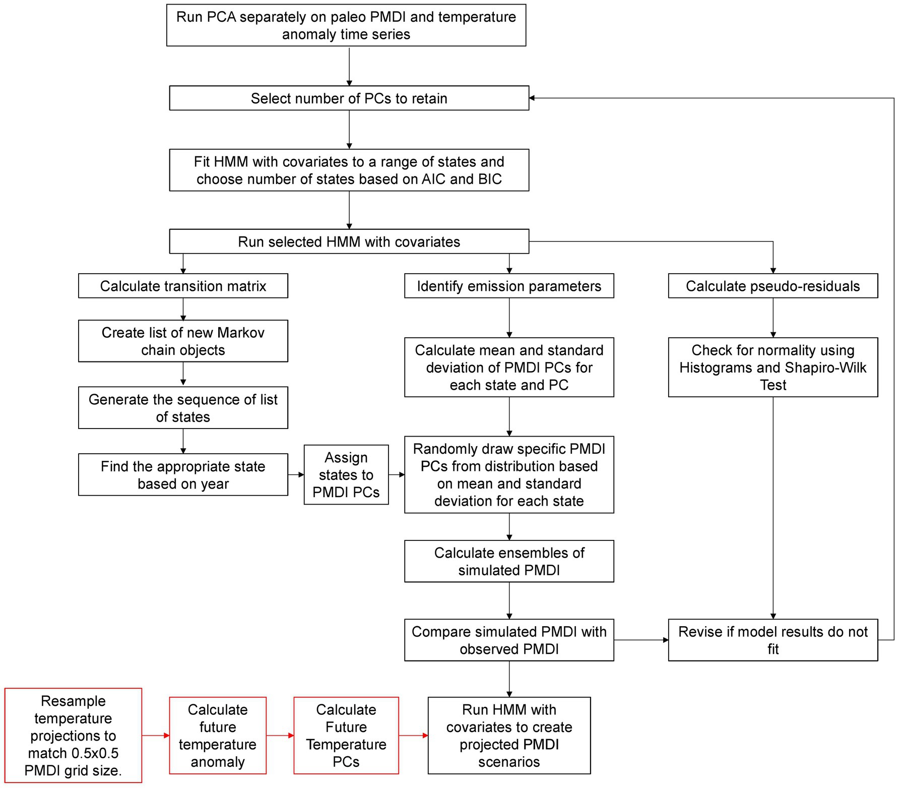
Figure 2. Flow diagram of methodology to fit, test and apply the HMM with covariates to PMDI. Red boxes represent steps involved in calculating future temperature PCs used to generate projections but not to fit and test the model.

2.3.1 Principal component analysis (PCA)

PCA is a multivariate technique that reduces a data set containing many variables to a data set having fewer new variables. These new variables are linear combinations of the original variables, and they have high variance while being uncorrelated with each other. The PCA method can compactly represent variability in atmospheric and other geophysical fields, which exhibit high correlations amongst variables (Wilks, 2019) and has been repeatedly applied in climate and hydrologic sciences to describe dominant patterns (Balling and Goodrich, 2007; Bethere et al., 2017; Lins, 1997). Researchers have used PCA to examine spatial variability of wet and dry periods (Eder et al., 1987; Raziei et al., 2008; Ogunrinde et al., 2020; Huang et al., 2022) while others have applied PCA for dimension reduction (Malmgren and Winter, 1999; Mortensen et al., 2018).

In this study, PCA is used to reduce the dimensionality of large paleo PMDI and paleo temperature records, increasing interpretability while minimizing information loss. The number of PCs is determined by calculating cumulative explained variance ratio, which is a function of the number of components. A scree plot is the common approach to depict this ratio and select number of PCs (Cattell, 1966). It displays the amount of variance captured by each PC in descending order, helping to identify the point where additional components offer diminishing returns in explained variance. To ensure that a sufficient proportion of the variance was captured, we chose to retain enough PCs to meet a minimum of 80% of variance explanation. This decision ensured that we captured sufficient variance while balancing the number of components included.

Figure 3 illustrates the methodological approach used in the study and illustrates how PCA reduces the dimensionality of the spatio-temporal reconstruction data. PCA decomposes spatio-temporal variability (Figure 3A) into temporal components (PC scores, Figure 3C) and their corresponding spatial components (loadings, Figure 3B). Note that while this illustration is generated using actual data, it is presented in a conceptual manner and does not show the specific PCs selected. The paleo PMDI data span from 1500 to 1980 with a matrix grid of 1823 × 481 (e.g., 1823 grid-cells and 481 years). Similarly, paleo temperature data covers the same period, arranged in a matrix grid of 1,637 grid cells by 481 years after resampling. The use of PCs in the HMM ensures that the primary variance in the data is retained while reducing its dimensionality, enabling more efficient analysis and interpretation.

Figure 3

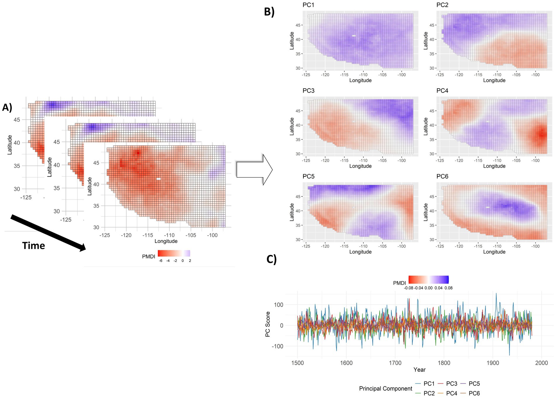
Figure 3. Conceptual illustration of the role of PCA in reducing dimensionality. (A) Spatio-temporal pattern of paleo PMDI data, (B) PC loadings for paleo PMDI data, and (C) Temporal variability in PCs. The gray rectangle area represents missing data.

To apply PCA, we took the set of PMDI time series, x, at locations 1 through M = 1823. We compute the eigenvectors of the data’s covariance matrix by singular value decomposition. The s-th PC (X_S) is then obtained using Equation 1:

\begin{array}{l} X_{s} = e_{s}^{T x'} = \sum_{m = 1}^{M} e_{m, s x m s=1, \dots, S} & (1) \end{array}

where e_s is the s-th eigenvector of the covariance matrix, x is the original data, and M is the number of variables (here locations). We repeated this process with the set of temperature time series y at locations 1 through M = 1,637. Then we retained the number of PMDI PCs, X, and temperature PCs, Y, sufficient to capture 80% of the variability for use in the HMM.

Autocorrelation, common in hydrological data, can lead PCA to detect of spurious spatial patterns (Planque and Arneberg, 2018; Vanhatalo and Kulahci, 2016). To assess whether autocorrelation impacts PCA results in this case, we conducted a comparative analysis of PCA on the PMDI with and without a pre-whitening procedure following Zamprogno et al. (2020). Minimal differences in the loadings and variance explained of the top 10 principal components confirm the acceptability of PCA on the original data in this case (see Supplementary material 1).

2.3.2 Hidden Markov model (HMM) with covariates

Hidden Markov models (HMMs) are statistical models that generate a variable sequence from a distribution based on the state of an underlying and unobserved Markov process (Zucchini et al., 2016). In the classical homogeneous HMMs, a system changes between unobserved or hidden states characterized by transition probabilities and a Markov chain. Each state corresponds to a probability distribution where observed time series are drawn (Bracken et al., 2014).

The time-homogeneity of the classical homogenous HMM can be limiting in practice if observations are non-stationary or have seasonal dependence. One approach to relaxing this assumption is making transition probabilities to be dependent on covariate time series, which is called a nonhomogeneous HMM (Hughes and Guttorp, 1994; Robertson et al., 2003; Bracken et al., 2016; Holsclaw et al., 2017; Steinschneider et al., 2019). Temporal inhomogeneity can also be introduced to the emission component of the model by allowing the parameters of the emission distributions to vary with time and location as a function of covariates (Holsclaw et al., 2017).

HMMs with covariates allow simulation of space–time realizations of a regional hydrologic process conditional on a sequence of atmospheric data. Analogously, we here create space–time realizations of PMDI conditional on temperature, which is physically linked to PMDI through atmospheric water demand. Furthermore, this enables the use of GCM temperature projections from climate scenarios to project the impacts of such climate changes on regional hydrological processes. Here, we adopt a Gaussian HMM with covariate Y (e.g., temperature PCs), which uses the temporal historical data X (e.g., PMDI PCs).

Once the model is fit, it can be applied to create an ensemble of space–time realizations of PMDI conditional on projected temperature changes by linking transition probabilities between states and emission distribution parameters to GCM generated temperature. An ensemble of state sequences is generated based on the transition probabilities by running the fitted HMM multiple times. Then, a unique mean and standard deviation are calculated for each location for a given state based on the projected temperature at that location and time (Figure 3).

Figure 4 shows the modelled dependencies between the PMDI PCs, X, hidden states C, and covariates Y in a graphical form, omitting, for simplicity, details such as relationships between different parameters of the model. Here, the temporal inhomogeneity is introduced in the emission component of the model by allowing the parameters of emission distributions $f (X_{t, s |C t} = k, μ_{t, k}, σ_{t, k})$ to vary with time t and principal components as a function of covariate Y (Holsclaw et al., 2016). In the function, k represents the state while μ and σ denote the emission parameters, which are mean and standard deviation, respectively (Equations 2 and 3).

Figure 4

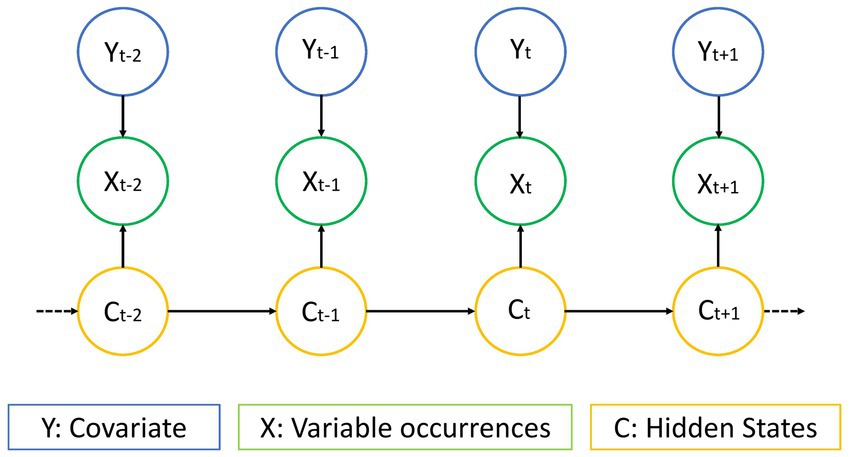
Figure 4. Structure of HMM. Y represents the covariate (additional variable, here temperature), X represents the variable occurrences (here PMDI), and C represents the number of hidden states (adapted from Zucchini et al., 2016).

The value for X for the s-th principal component s = 1, …, S at year t = 1, …., T, conditioned on the hidden state variable C = k, is modelled via independently Gaussian distributed variables with mean and standard deviation:

\begin{array}{l} P (X_{t, s |C t} = k, \dots) = N (X_{t, s} | μ_{t, k, s}, σ_{k, s}) & (2) \end{array}

\begin{array}{l} μ_{t, k, s} = \sum_{i = 1}^{n} δ_{i, k} Y_{i, t} & (3) \end{array}

Where:

• $N (X_{t, s} | μ_{t, k, s}, σ_{k, s})$ represents Gaussian distribution with mean μ and standard deviation σ

• $μ$ is the function of the time-varying covariates $Y_{t}$ (temperature PCs) as well as the state (k) and X (s)

• $δ_{i, k}$ is the coefficient for covariate i at state (k)

• n is the number of covariate variables (here the selected number of temperature PCs)

• σ is function of the state (k) and X (s)

This approach enables the model to account for temporal variations in the emission process, improving its flexibility and accuracy in capturing the dynamics of wet and dry events via PMDI.

The HMM model with covariates is fitted for a specified number of states using the Expectation–Maximization (EM) algorithm (also called the Baum-Welch algorithm). Once the model is fit, the Viterbi algorithm is then employed to identify the most likely sequence of states. Then Bayesian Information Criterion (BIC) and Akaike’s Information Criterion (AIC) are used to select the appropriate number of states. BIC seeks to maximize model consistency while AIC seeks to maximize model efficiency (Celeux and Durand, 2008). There are theoretical questions about the use of BIC and AIC in this context. While BIC tends to underestimate the number of hidden states, AIC demonstrates a tendency to overfit the number of hidden states in an HMM (Celeux and Durand, 2008; Buckby et al., 2020). The appropriate number of hidden states in an HMM can be determined by the minimum BIC or AIC value (Bacci et al., 2014). However, both AIC and BIC can be used to determine a range of plausible model sizes by model averaging (Dziak et al., 2020). Here, we select a mid-point of hidden states of models to balance the goals of efficiency and consistency. If the two metrics disagree, rounding down to the nearest integer can be applied for computational efficiency.

To assess whether the fitted model describes the data well, a comprehensive comparison between model simulations and the observed data for the paleo PMDI data is conducted using both visually (e.g., time series plots, spatial maps, residual plots, and histograms) and statistically by quantifying the goodness-of-fit, such as the root mean square error (RMSE). Furthermore, pseudo-residuals (also known as quantile residuals) are calculated as an additional check on model performance based on the information provided following the procedure detailed by Zucchini et al. (2016). This cannot be done by analyzing only standard residuals because the observations are explained by different distributions depending on the active hidden state. Following Zucchini et al. (2016), we conclude that the observations are modeled well if pseudo-residuals are close to standard normal distribution. We visually assessed the residuals and pseudo-residuals using histograms and statistically using the Shapiro–Wilk normality test (Shapiro et al., 1968).

Following set up and testing, the HMM with covariates is applied to generate an ensemble of spatially explicit PMDI historic simulations and projections. To generate an ensemble, the model is iteratively run, with each run resulting in a sequence of states. Additionally, the emission parameters are identified for each state and year (as temperature, the covariate, is time-varying). The emission parameters define the Gaussian distribution for each state and year. For each time step in each sequence the distribution is sampled for the PMDI PCs. These simulated PMDI PCs are then multiplied by their respective loadings to obtain the spatially explicit simulated PMDI. Importantly, as HMM with covariates is a stochastic model, the results will vary with each run, which reflects the inherent variability and uncertainty in the system. The framework extends to future projections by using temperature projections for the covariate.

3 Results

The results of HMM with covariates after PCA, including model development, selection, pseudo-residuals assessment and application are given in this section.

3.1 PCA

The scree plot and the cumulative variance plot criterion are used to choose the appropriate number of PCs (Supplementary material 3). The scree plot suggests selecting 4 PCs, as the variance explained began to plateau at that point. However, we chose to retain 6 components because they collectively explained a minimum of 80% of the variance. Consequently, the first six PCs are selected both for paleo PMDI and paleo temperature data, as they capture a significant portion of the variance before the curve plateaus. Specifically, the 6 PCs account for 81.4% of the variance in the paleo PMDI data and 84.6% of the variance in the paleo temperature data.

3.2 Hidden Markov model with covariates

Nine HMMs with covariates are fitted to the data with a range of states from two to ten. The minimum BIC is calculated at state two and the minimum AIC is found at state six. The HMM model with four hidden states for the entire study area is selected as the optimal model, representing a balance between efficiency and consistency, as it is the mid-point between the minimum AIC and BIC values (Table 2).

Table 2

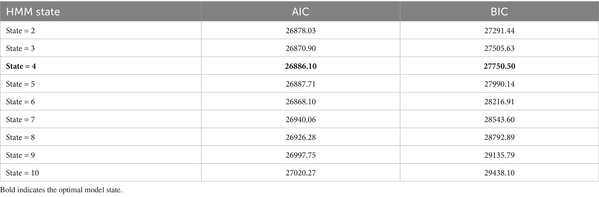
Table 2. HMM with covariates model selection.

For the selected four-state model, Figure 5 shows the paleo PMDI and paleo temperature anomaly time series, averaged across the study area, together with most likely hidden states over the Western U.S. during training period. Positive PMDI represents wet conditions while negative PMDI represents dry conditions. Figure 5 illustrates the connection between observed PMDI, observed temperature anomalies, and the corresponding states identified by the model. Figure 5 further illustrates the value of using the paleo record in this analysis as evidenced a larger range of PMDI than observed over the instrumental record. For example, during the decades 1548–1558 and 1817–1826, PMDI values consistently fell below -1 across several locations in the northern and central Great Plains, which indicates sustained and regionally extensive drought conditions. These prolonged drought conditions emphasize the severity and persistence of naturally occurring hydroclimatic extremes, which are not captured in the shorter instrumental record.

Figure 5

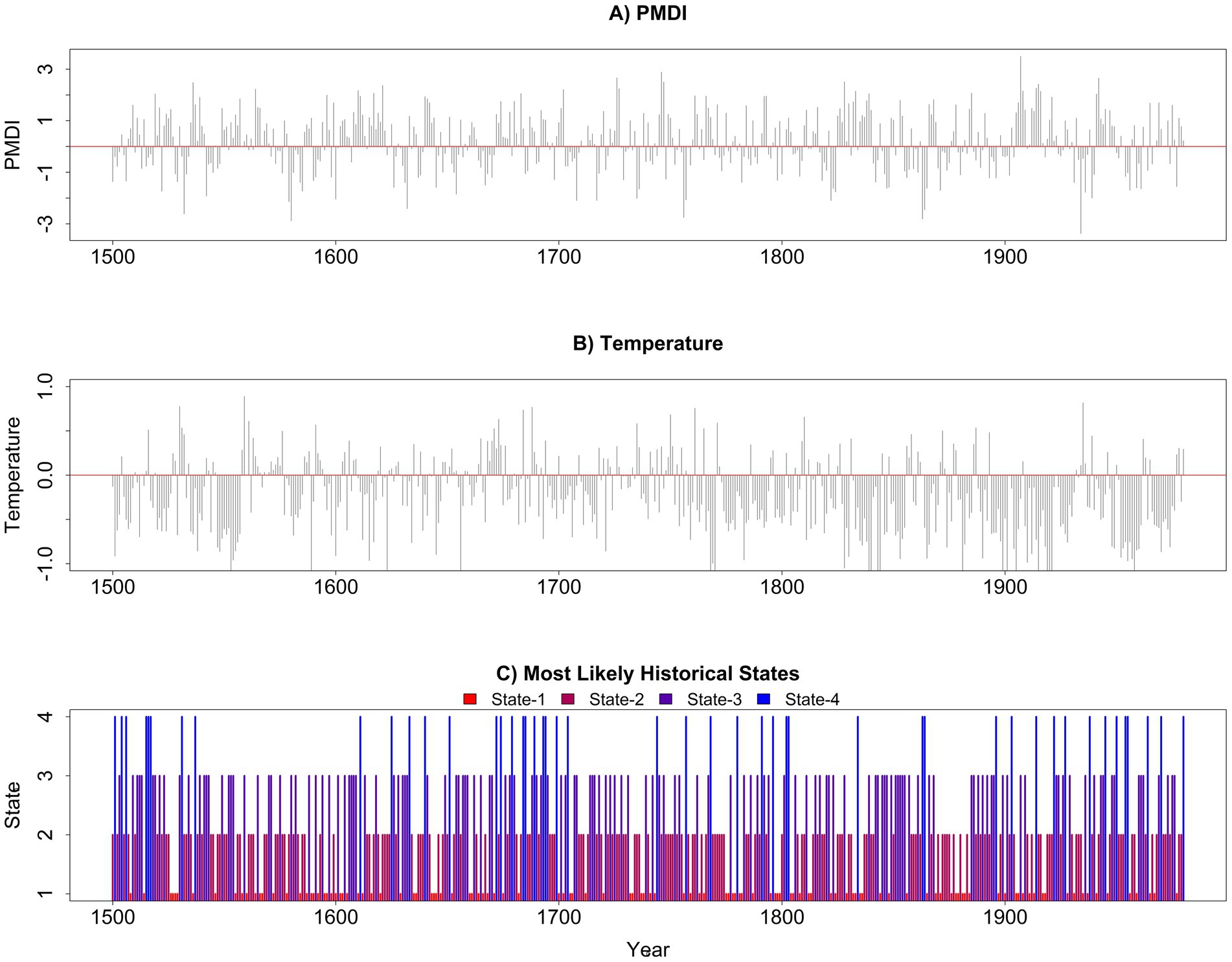
Figure 5. (A) Annual mean paleo PMDI time series over the Western U.S., (B) Annual mean paleo temperature anomaly time series over the Western U.S., and (C) Most likely states over the Western U.S.

Figure 6 shows the comparison of observed mean paleo PMDI and ensembles of simulated mean PMDI over the study area. The observed mean paleo PMDI falls within the range of the simulated ensembles, indicating that the simulations capture the overall variability and trends. The performance of the ensembles is evaluated using the RMSE. The RMSE values of the ensemble models are predominantly concentrated in the range of 1.5 to 1.6. Although the model is stochastic and does not aim to reproduce the specific observed sequence, approximately 65 out of the 100 ensembles fall within this range, indicating a high consistency in model performance. Furthermore, the Shapiro–Wilk test is applied to the pseudo-residuals and p-values for pseudo-residuals are found to be greater than the chosen alpha level of 0.05, which confirms the normality of the pseudo-residuals.

Figure 6

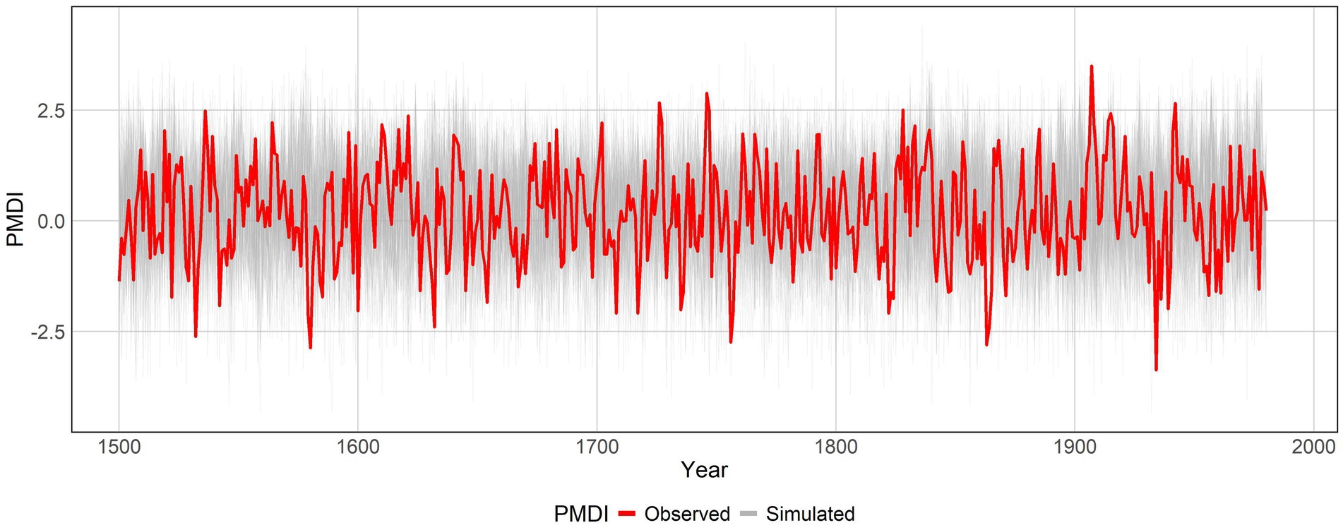
Figure 6. Observed mean paleo PMDI and 100 ensembles of simulated mean PMDI over time.

A traditional HMM approach without a covariate is also applied to simulate ensembles of mean PMDI over the study area. The historical record is divided into two parts: the first 70% (1500–1835) is used to develop both traditional HMM and HMM with covariates generators, while the remaining 30% (1836–1980) is used as a validation period to assess models’ ability to produce synthetic PMDI data. The model results show that the HMM with covariates has a very low mean bias (0.003) for the recent observed period. However, the traditional HMM bias, while still low, shows a higher mean bias (0.09), indicating that including temperature as a covariate reduces the bias. While both models demonstrate high consistency in their simulations, the HMM with covariates is selected in this study since it can incorporate external covariates, such as temperature PCs, into the model. The HMM’s capacity to incorporate covariates enables the generation of future scenarios that are directly informed by projections of those covariates (e.g., CMIP6 surface temperature from GCMs). Details of the traditional HMM approach can be found in the Supplementary material 2.

The model provides insight into hydroclimatic regimes (e.g., recurrent spatial patterns) or states via independently Gaussian distributed variables with mean and standard deviation where both mean and standard deviation are unique to each PC for a given state. Figure 7 illustrates the simulated PMDI reconstruction patterns and state transition probabilities when there is no temperature impact on PMDI (e.g., temperature anomaly is zero). Figure 7 shows the spatial patterns of PMDI associated with the four states, and the likelihood of transition from each state to all other states. The wettest state is identified as state 4 with the highest percentage of wet area (W = 99.5%) and the driest state is determined as state 1 with the highest percentage of dry area (D = 73%). These states represent data-driven patterns derived from the model, captured PMDI variability influenced by global climatic cycles (e.g., El Niño/Southern Oscillation, Pacific Decadal Oscillation) and regional climate dynamics.

Figure 7

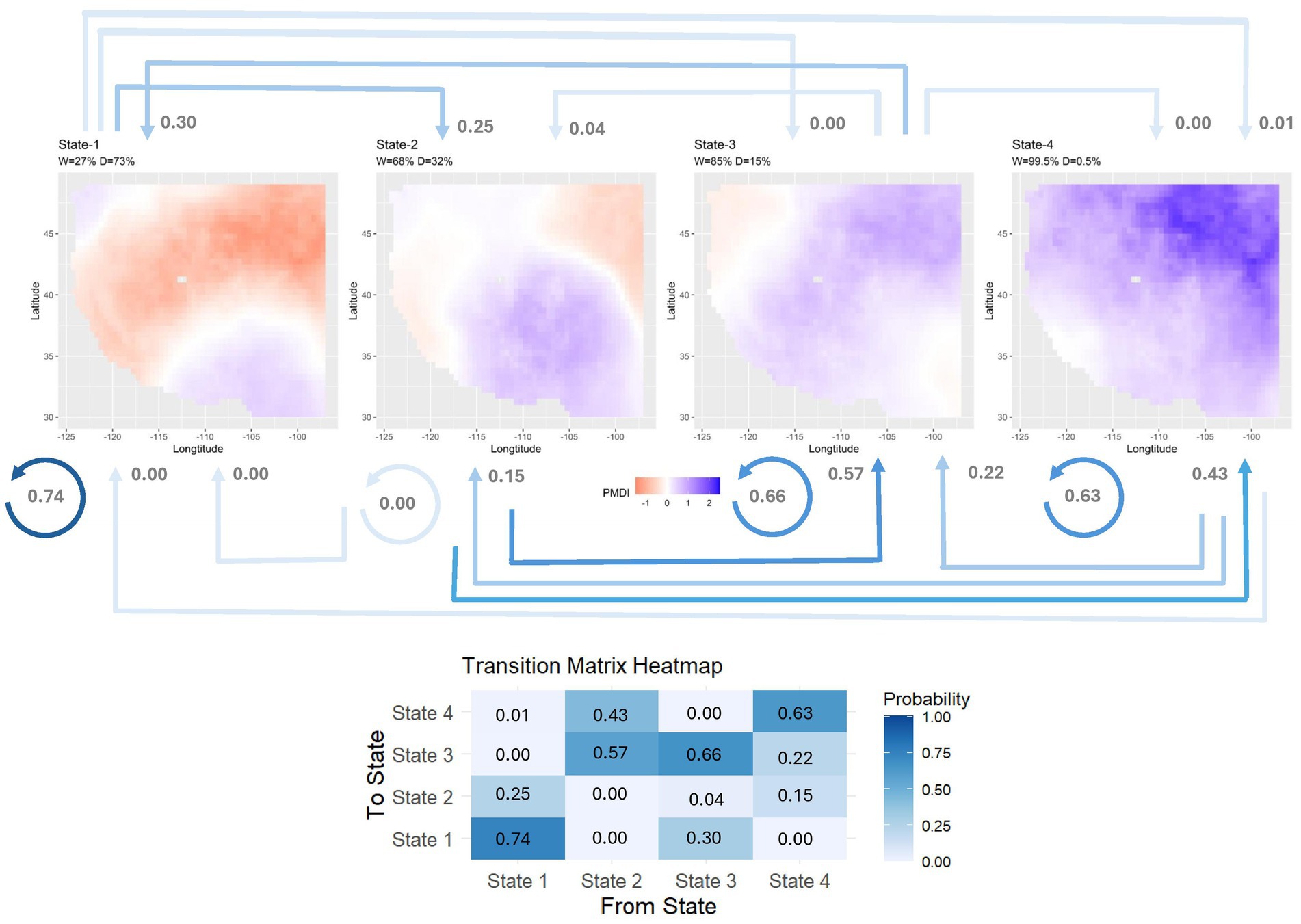
Figure 7. Annual mean PMDI reconstructions in each hidden state when temperature anomaly is zero. Blue represents a positive anomaly (e.g., wet) while red represents a negative anomaly (e.g., dry) of PMDI. “D” (dry) is the percentage of the area where mean PMDI reconstructions are less than zero and “W” (wet) is the percentage of the area where mean PMDI reconstructions are greater than zero. Transition probabilities are shown as a heatmap, arrows represent transition directions and match the colors in the heatmap. The gray rectangle area on the map represents missing data.

The transition probabilities help to identify how states can be expected to shift to either a wet or dry state in the next year. For example, the probability of state 3 occurring the year after state 2 is 0.57. However, state 1 shows the highest persistence with a probability of 0.74 to remain in the same state from year to year. This indicates that the study area is more likely to experience persistent region wide dry conditions. On the other hand, state 4 has a transition probability of 0.63 for remaining in the same state and 0.22 probability of transitioning to the moderately wet state 3 in the next year. This indicates that once the study area is in the wettest state, it is more likely to stay wet rather than shifting to a dry state.

Given the model developed for the historic training period, one can generate plausible sequences of hidden states for the forecast period. Figure 8 illustrates one stochastic scenario of system states (e.g., scenario 1) at each time step during the forecast period. For example, the first scenario shows no single state dominating during the early period (2020–2040). As we moved into the mid and late 21^st century, State-3 is more dominant in this scenario. Moreover, ensemble-based analysis reveals that the persistence of drought events is anticipated to intensify significantly in the future period. While historical droughts lasted an average of 11.5 years, future droughts are expected to persist for an average of 33.18 years, indicating prolonged drought events under the SSP 245 scenario.

Figure 8

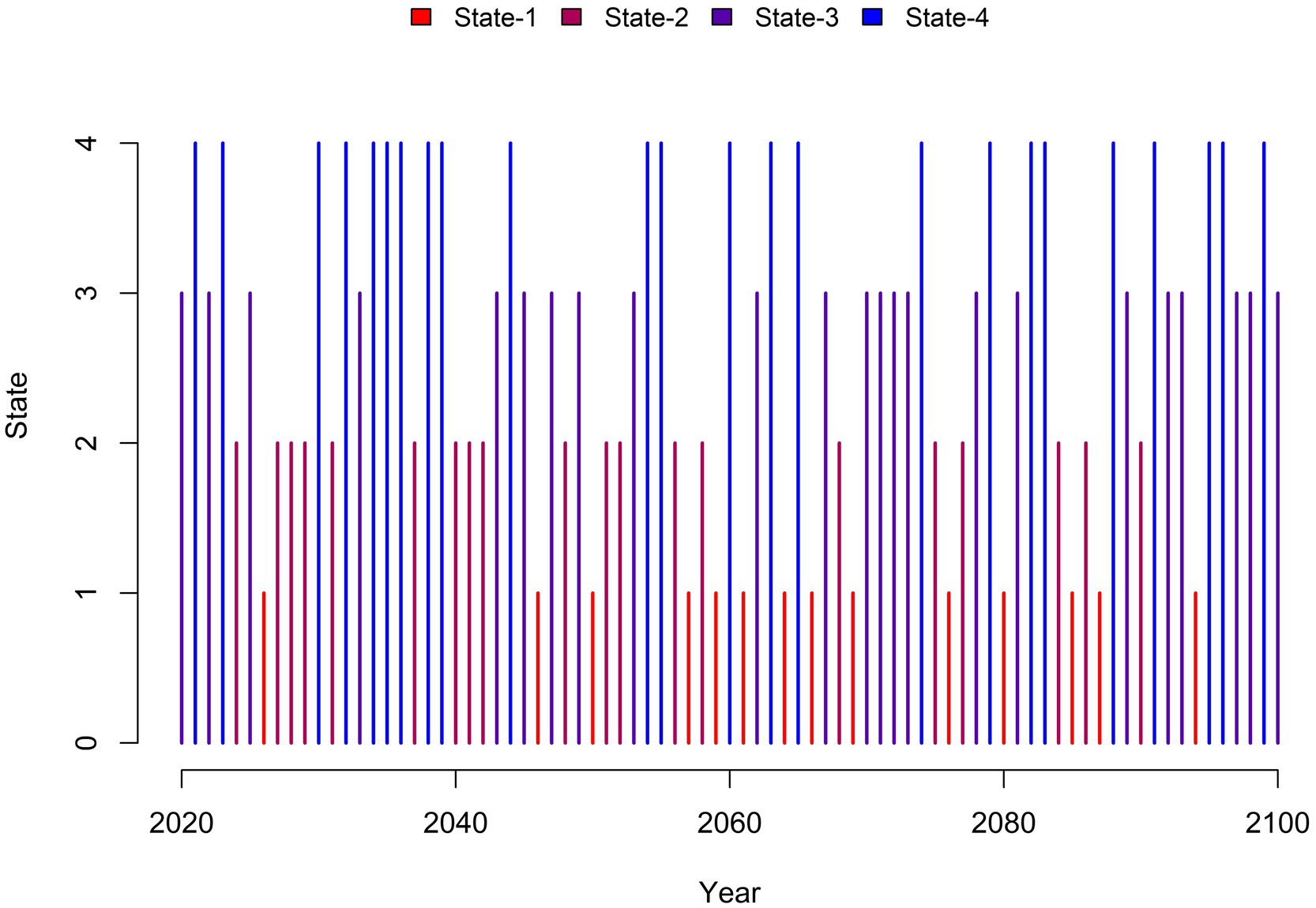
Figure 8. One stochastic scenario of system states in the Western U.S. (Scenario-1).

Future PMDI scenarios, informed by a specific temperature scenario, are created from 2020 to 2100 for the Western U.S. using the model. Figure 9 shows the spatial pattern of annual temperature reconstruction anomalies and simulated median PMDI reconstructions across ensembles in the study area for one historic and one projected year. The annual temperature anomaly significantly rises by the end of the century all over the Western U.S. under the SSP 245 scenario. Corresponding to the temperature increase, the median PMDI reconstructions show a shift from relatively neutral conditions in 1500 to widespread drought conditions in 2100. Analysis of the ensemble results further reveals that the spatial extent of drought is expected to expand dramatically, with the proportion of affected grid cells increasing from 8.84% during the historical period to 51.1% during the future period under SSP 245 scenario. While Figure 9 illustrates just one PMDI scenario from the ensemble, it exemplifies the positive correlation between rising temperatures and dry conditions in the Western U.S.

Figure 9

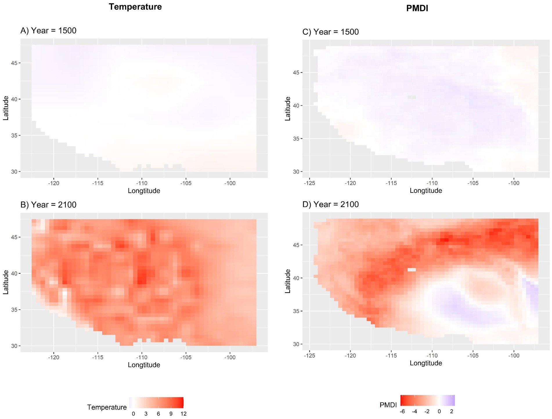
Figure 9. Spatial comparison of (A) Annual paleo temperature anomalies in 1500, (B) Annual temperature anomalies in 2100, (C) Simulated median PMDI reconstructions across ensembles for 1500, and (D) Simulated median PMDI reconstructions across ensembles for 2100 in the Western U.S. The gray rectangle area represents missing data.

Quantile ranges for an ensemble of 100 projected sequences over time for the case study area are shown in Figure 10. The figure shows changes in PMDI variability of each 100 scenarios over time. According to Figure 10, the PMDI variability over the Western U.S. is likely to increase over time under the SSP 245 scenario due to increase in temperature variability. The standard deviation of temperature shows a significant increase from the historical period, ranging from 1.1574 to 1.1989, to the future periods, with values between 1.661 and 1.803 for 2020–2060 and 1.631 to 1.804 for 2060–2100. This increase in temperature variability directly contributes to the rising PMDI variability. The increasing range and decreasing mean of PMDI suggests a significant influence of temperature changes, specifically as we move into the mid to late 21^st century. This variability points to a higher likelihood of more extreme drought events and greater uncertainty in wet and dry conditions. The broader range of PMDI values during this period indicates that the impacts of climate change, particularly rising temperatures, are likely causing more frequent and severe droughts, but also some extreme wet years. For example, only 8.7% of drought events [PMDI<= − 2; National Centers for Environmental Information (NCEI), 2024] were identified between 1500 and 1980. However, projections for the period from 2020 to 2100 indicate a sharp rise, with drought occurrences expected to increase to 50%. This highlights a significant increase in the frequency of drought conditions in the future under SSP 245 scenario. Furthermore, the mean PMDI shows a tendency to decrease over time, indicating regional aridification as we move towards the end of the century. This trend is explained by increasing air temperatures, which enhances evapotranspiration rates and reduces soil moisture, leading to lower PMDI values.

Figure 10

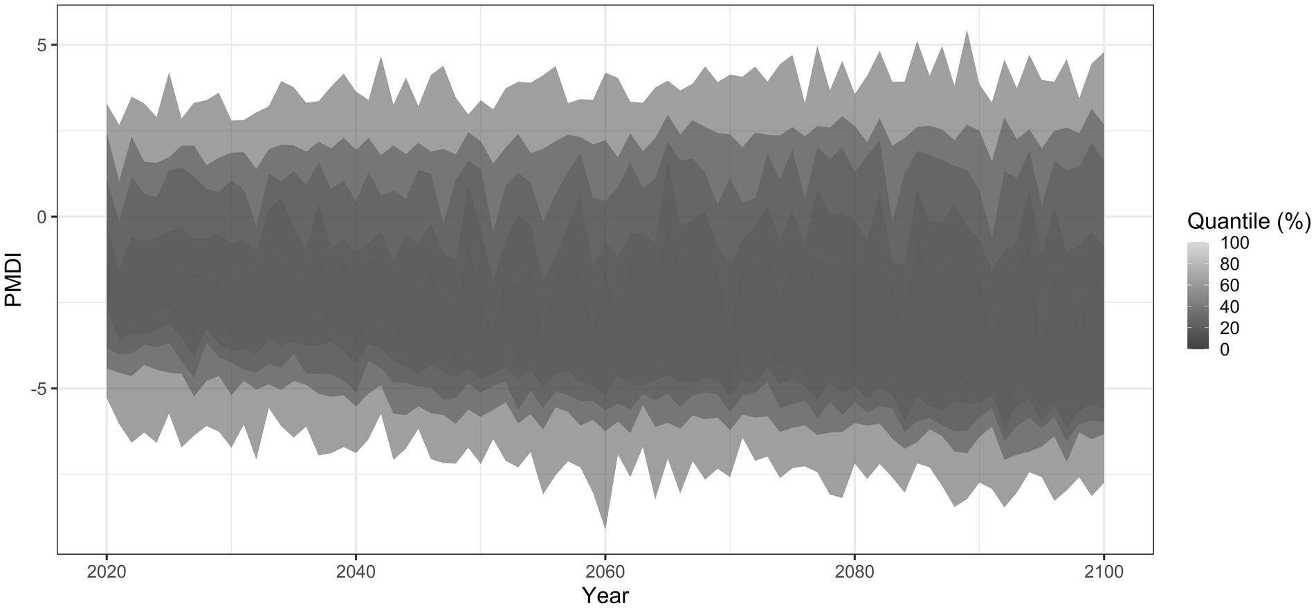
Figure 10. Quantile range for ensemble of 100 sequences of scenarios of PMDI spatially average across the study period the Western U.S. Darker areas represent higher densities of data points, while lighter areas indicate less frequent occurrences.

4 Discussion

This study used a HMM with covariates to create future PMDI scenarios over the Western U.S., incorporating temperature projections as the covariates. The methodology incorporates the integration of HMM with covariates and PCA to efficiently handle high dimensional paleoreconstruction data, enabling the generation of robust future climate informed scenarios. The approach successfully captures the spatiotemporal variability and regime-shifting behavior of climatic patterns, providing critical insights for spatial correlation of wet and dry conditions across the regions of the Western U.S. Key findings from the study highlight several important aspects of climate dynamics in the Western U.S.

The HMM with covariates effectively models the regime-shifting behavior in climatic patterns by identifying wet and dry states. Transition probabilities between these states reveal the likelihood of shifts, aiding in the understanding of the persistence and variability of drought conditions. For example, Figure 7 provide a detailed view of how wet and dry states are distributed, highlighting the persistence and variability of climatic patterns across the Western U.S. The maps reveal that certain climatic conditions, whether wet or dry, can persist over several years, which is critical for understanding long-term water availability and water planning. The insights gained from the model results are valuable for water resource managers and policymakers, enabling better anticipation of periods of water surplus or shortage and informing decisions on water storage, allocation, and conservation measures to ensure a resilient water supply system.

One of the key advantages of this study is that the developed model has the ability to make temperature informed PMDI projections. Using climate-informed variables (e.g., temperature) as covariates can help capture the variations in a hydrological variable (e.g., PMDI) that are influenced by the covariates through physical processes. Thus, utilizing a climate informed covariate increases the model skill in capturing persistence and nonstationary (Ho et al., 2018; Vinnarasi and Dhanya, 2022). In this study, incorporating temperature PCs as a covariate significantly enhances the model’s projections. The decision to use only temperature data as a covariate is supported by the consistent role of temperature in driving drought conditions in our study area; further, precipitation projections from GCMs still exhibit significant biases in climatology and variability, and therefore adding precipitation as a co-variate could add error (Kunkel et al., 2020; Srivastava et al., 2020). Additionally, PMDI already incorporates key climate variables such as precipitation, temperature, soil moisture, and evapotranspiration to assess long-term drought and moisture conditions. Temperature also has well-documented paleo data; it serves as a reliable input for historical period. Conversely, variables like precipitation, soil moisture and evapotranspiration lack corresponding paleo records, making them unavailable for the historical period we analyzed. As shown in Figure 10, the developed model can capture nonstationary by allowing the parameters of the emission distributions to vary with time as a function of a covariate. The wide range of PMDI variability over time shows that the severity of wet and dry events over the Western U.S. is likely to increase by time under the SSP 245 warming scenario applied. Additionally, the findings highlight the critical impact of rising temperatures on regional aridification, with decreasing tendency of mean PMDI over time towards the end of the century under the SSP 245 scenario. These findings enhance our understanding of how uncertainties in air temperature impact PMDI variability, providing valuable insights into the future climate dynamics of the region. Furthermore, the heightened variability underscores the challenges for water resource management, necessitating adaptive strategies to manage extreme conditions.

Having relatively short instrumental records is a key limitation to assess spatial patterns in wet and dry periods in the U.S. for long time scales. Paleoreconstruction data offer a long-term perspective on climatic variability by supplementing relatively short observation data (Ho et al., 2018). Annually resolved paleoclimate records provide a framework for exploring policy and management alternatives to mitigate or adapt the future changes [U.S. Geological Survey (USGS), 2022]. This study effectively utilized long-term paleoreconstructions to overcome the limitations posed by relatively short observational records. As depicted in Figures 5A,B, this study leveraged PMDI and temperature paleoreconstructions to train the HMM, enabling the model to simulate a wide range of spatio-temporal climate informed scenarios (Figure 10), thereby enhancing its reliability and applicability. Utilizing long-term paleoclimate records enables us to better understand the long-term climate variability over time scales relevant to water resources management and planning to mitigate or adapt to future changes by creating ensemble of scenarios.

Given the high dimensionality of the paleoreconstruction data, PCA is applied to reduce the dimensionality of data and thereby enable computationally efficient HMM. Precisely, the computation time is 7 min for the model to generate an ensemble of 100 sequences of scenarios. All experiments are run on a 64-bit computer with Intel(R) Core (TM) i7-8665U CPU @ 1.90GHz 2.11 GHz processor and 32 GB of RAM running Windows 10 Enterprise. The developed model shows a strong performance in simulating paleo PMDI data, as seen in Figure 6 by the alignment of observed and simulated mean PMDI, and the normality of pseudo-residuals. Another advantage of developing the HMM with PCA output in comparison to other dimensional reduction techniques such as clustering, is its grid-based representation, which provides insight into wet and dry events by representing a specific PMDI value at a given time and state. As shown in Figure 9, the ability to have grid-based representation is of interest for local and regional resource managers since it generates realistic and spatially variable scenarios.

Another advantage of our approach is its ability to estimate uncertainty in natural variability via HMM framework, which is more computationally efficient compared to running a single-model initial condition large ensemble (SMILE). While SMILEs involve running multiple ensemble members initialized from slightly different conditions to capture variability, this method is computationally expensive, specifically for large-scale climate projections (Lehner et al., 2020). In contrast, our approach can compare insights by modelling regime-switching behavior through hidden states that represent different climate regimes (e.g., wet and dry periods). Additionally, the model can capture the inherent natural variability without requiring multiple runs of climate models. This efficiency could be particularly beneficial when computational resources are constrained.

Although the recent generation of models in CMIP6 offers improved resolutions (Liang-Liang et al., 2022), GCMs may still be inadequate for providing the detailed regional information required for climate change impact studies, particularly at the river basin scale (Banda et al., 2022). The HMM simplifies the temporal and spatial structures to be parameterized despite its large number of parameters and computational complexities (Mehrotra and Sharma, 2005). As seen in Figures 9D, 10, the study presented here can avoid these issues, creating 0.5 × 0.5-degree grid cell coverage ensemble of future PMDI scenarios from year to year at each grid location by linking the model with covariates (e.g., bias-corrected 1.25 × 1.25 grid spacing CMIP6 surface temperature data) and using computationally efficient model as mentioned above paragraph.

According to GCM outputs and detailed regional studies, streamflow is sensitive to changes in temperature and precipitation but the regional impacts of global warming on future water supplies are uncertain (Frederick and Gleick, 1999; Lehner et al., 2019). For example, McCabe and Wolock (2007) showed that 1°C to 2°C increases in temperature could result in substantial water supply shortages in the Upper Colorado River Basin. They also reported that future warming could increase the probability of failure to meet the water allocation requirements of the Colorado River Compact. Creation of ensembles of regional climate scenarios is necessary for the quantification of climate uncertainty in the influence of global warming to address the potential impacts of climate change and climate variability on future infrastructure planning and water policy (Groves et al., 2008). One of the significant contributions of the paper is that the developed model generates an ensemble of plausible future regional PMDI scenarios for any projected temperature sequence, as presented in Figure 10. These ensembles can be helpful for water resources managers, infrastructure planners, and government policymakers tasked with infrastructure planning and building of more resilient communities. Moreover, streamflow ensembles that preserve long-term spatio-temporal variability can be generated by using these ensembles. Prior research has demonstrated several feasible ways to do this including stepwise multiple linear regression, PCA and canonical correlation analysis (Barnett et al., 2010; Day and Sandifer, 2015). Thereby, these ensembles can play a pivotal role to address creating inter-site and inter-basin streamflow reconstructions (Ho et al., 2016) for better water supply management of interconnected networks of watersheds.

An important limitation of this study is that paleo PMDI and paleo temperature data are based on tree-ring chronologies, and the uncertainty increases with the age of the chronology due to lower tree-ring sample availability. Therefore, the accuracy of the fitted HMM and subsequent state and emissions distributions are affected by the uncertainty of the reconstructed input data. Furthermore, both paleo PMDI and paleo temperature records do not include climate variables like net radiation or wind speed, which may also play a crucial role in influencing future drought occurrences and intensities (Brunner and Gilleland, 2024). However, the advantages of using paleo PMDI and paleo temperature are specifically the ability to train a model on a wider range of hydrological conditions and spatial patterns motivate use of this data despite the limitations.

In future research, the methodology developed here could also be applied using other hydroclimatic metrics, depending on the application of interest. This approach can be used for any region or watershed to better understand the spatio-temporal patterns of drought events. An ensemble of plausible future regional PMDI scenarios can be used to inform watershed or regional planning and decision making. Furthermore, these ensembles can be used to generate streamflow ensembles, which, in turn, will be a valuable input to study the impact of climate change on regional hydrology and water management. Additionally, future work could focus on computing PMDI from climate projections to assess whether the statistics align with those from the non-stationary generator. This comparison would demonstrate the consistency of the analysis with a large ensemble of PMDI values, making it a clearly chosen option.

Data availability statement

Publicly available datasets were analyzed in this study. The paleo data can be accessed at: https://www.ncei.noaa.gov/access/paleo-search/. Temperature projection data is cited within the manuscript. Model code and processed data are available at Tezcan and Garcia (2025).

Author contributions

BT: Conceptualization, Data curation, Formal analysis, Investigation, Methodology, Software, Validation, Visualization, Writing – original draft, Writing – review & editing. MG: Conceptualization, Funding acquisition, Investigation, Methodology, Project administration, Supervision, Writing – review & editing, Writing – original draft.

Funding

The author(s) declare that financial support was received for the research and/or publication of this article. This work is funded by the National Science Foundation (CIS-1942370).

Conflict of interest

The authors declare that the research was conducted in the absence of any commercial or financial relationships that could be construed as a potential conflict of interest.

Publisher’s note

All claims expressed in this article are solely those of the authors and do not necessarily represent those of their affiliated organizations, or those of the publisher, the editors and the reviewers. Any product that may be evaluated in this article, or claim that may be made by its manufacturer, is not guaranteed or endorsed by the publisher.

Supplementary material

The Supplementary material for this article can be found online at: https://www.frontiersin.org/articles/10.3389/frwa.2025.1472695/full#supplementary-material

References

Adamowski, J., Adamowski, K., and Prokoph, A. (2013). Quantifying the spatial temporal variability of annual streamflow and meteorological changes in eastern Ontario and southwestern Quebec using wavelet analysis and GIS. J. Hydrol. 499, 27–40. doi: 10.1016/J.JHYDROL.2013.06.029