Spatial distribution and source identification of metal contaminants in the surface soil of Matehuala, Mexico based on positive matrix factorization model and GIS techniques

1. Introduction

One of the most essential eco-environmental systems for human existence and prosperity is the soil, and soil sustainability is an important assurance of both global food security and the wellbeing of humans (1–4). Soil pollution, particularly soil heavy metal contamination and deposition, has become a severe and environmentally critical issue. Therefore, it’s receiving a lot of public attention due to societal concerns (5–9). Since Mexico is a developing country that has recently considered significant urban development, soil contamination by heavy metals has emerged as a serious environmental issue (10, 11). The Comarca Lagunera area, which covers the northern Mexican states of Coahuila and Durango, first became aware of the issue of arsenic (As) and other heavy metal contamination due to its excessive concentrations in the sedimentary aquifer in 1958 (12–14). In the City of Torreon in Mexico, 40 incidents (including 1 death) of As-related health problems were reported in 1962 (15). Some of these recorded incidents might be thought of as the beginning stages of As and other heavy metals-related environmental, geochemical, and medical investigations in Mexico (14). Heavy metal extraction from various mining waste materials, and exposure through smelting dust and fumes, including its distribution, were all explored at various mining and ore processing sites in the regions of Baja California, Guerrero, Guanajuato, Hidalgo, and San Luis Potosi (16–19). In the San Luis Potosi area, soil contaminated by heavy metals from the dissolution of natural metal sources could be distinguished from various sources with metal contamination originating from tailings by chemometric and isotopic approaches (20–22). Metal contaminants may also rapidly translocate and concentrate in the food chain posing substantial concerns to food security and human wellbeing (23–26). In fact, quantitative evaluations of the properties, toxicity, and origins of heavy metals in soil are essential for public safety. Therefore, metal contamination in soils might be a prominent indication of the influence of anthropogenic activities.

The different techniques were utilised to determine the distinctive distribution patterns and sources of metal contamination in soils, including geographic information system (GIS), positive matrix factorization (PMF), and principal component analysis (PCA) (27–31). To identify the source contributions, standard source apportionment procedures (e.g., PCA and PMF) and contamination monitoring techniques (e.g., contamination indices and ecological risk factors) are often implemented (32–36) and estimate the risk of metal contamination in soils, accordingly (37–40). However, several contamination indices such as the geo-accumulation index (I_geo), contamination factor (C_f), pollution load index (PLI), degree of contamination (C_d), potential ecological risk index, Nemerow’s Pollution Index (PI_N), and human health risk assessment analysis (carcinogenic and non-carcinogenic risks) were used to assess heavy metal contamination in soils systematically (19, 41–44). In general metal contamination in soils is derived from two major sources: natural (e.g., soil mineral and organic components) and anthropogenic sources (e.g., agricultural activities, transportation, mining activities, industrial activities, etc. However, it is critical to differentiate contamination sources qualitatively and quantitatively in order to preserve the soil ecosystem (45–49). A common approach for distributing metal contamination sources is to perform multivariate receptor models, which don’t even require prior information on source characteristics (50). The source identification of metal contamination in soils, various hybrid receptor models, especially partition computing based positive matrix factorization (PC-PMF), absolute principal component score-multiple linear regression (APCS-MLR), GeogDetector models, multivariate curve resolution-weighted alternating least squares (MCR-WALS), and UNMIX have been commonly implemented (4, 50–54). The significant disadvantage of using a receptor model for metal contamination source identification is that the approach does not usually satisfy certain key assumptions (55, 56).

The positive matrix factorization (PMF) model is a mathematical matrix decomposition approach that can manage insufficient and imprecise data by applying non-negative constraint criteria. This model is a common receptor model which has been frequently utilised for the identification of the source of metal contamination in the atmosphere, sediment, and soil (31, 57, 58). However, the PMF model is empirical in identifying sources of contamination and assumes contaminant spreads as a linear process (56, 59). Hence, it discards critical information detailed in the spatial correlation between soil samples. Unfortunately, the PMF model may have uncertainties, which might cause some inaccuracies in the source apportionment results (60, 61). The study by 62 describes that data inconsistency, model structural disintegration, and model parameter accuracy are the three key factors contributing to uncertainty in PMF source identification. In most cases, data inconsistency is related to quantitative measuring errors and sample data inaccuracies. To assess the impact of stochastic errors and a limited small amount of factorization in uncertainty analysis on the PMF result, the essential bootstrap approach can also be applied (61, 63, 64). Therefore, it is relevant to evaluate the variation of uncertainty in PMF models.

This study was designed to ascertain the concentrations of heavy toxic metals (e.g., As, Sr, Mn, and Fe) and light metals (e.g., Ca, Mg, Na, and K) contamination in recreational and agricultural surface soil of Cerrito Blanco area in Matehuala municipality, San Luis Potosi, Mexico and to explore the factors that affect the spatial distribution and source identifications. The previous studies done in this particular region established Cd, Cu, Cr, Zn, or Pb as primary contamination risk factors (19, 22, 65, 66). Therefore, these heavy metals were not repeated for this study. The other reasons for choosing these metals found in this same region are because of historic mining activities and the data availability. Thus the main objectives of this study were as follows: (i) to examine the significant relation between soil-metals concentration and the spatial distribution of contamination sources from hazardous areas; (ii) to evaluate the source apportionment by identifying the different factors of metal contamination in the surface soil using PMF model; (iii) to assess the contamination risk levels based on different types of contamination indices in the surface soil; and (iv) to classify the spatial distribution patterns of metals contamination and pollution source identification factors based on IDW interpolation techniques.

2. Study area

In this study, two locations were selected from the abandoned past mining and smelting areas surrounded by recreational non-cultivated, and agricultural farmland in the northeastern part of Matehuala municipality named Cerrito Blanco, San Luis Potosi, Mexico. This study area is divided into two parts according to soil sample characteristics, study area 1 refers to recreational soil, and study area 2 represents agricultural soil. The study area is located between 23°40′30′′ N latitude and 100°35′27′′ W longitude, having a total geographical area of approx. 4.84 ha (Figure 1). Study area 1 refers to a soccer club, also known as Joya Verde soccer sporting club. This club has been in use for around 18 years and was constructed on land that was communally owned and utilised for farming between 1974 and 2003 (67). It consists of three half-hectare soccer fields surrounded by sparsely vegetated areas identified as non-irrigated undeveloped cultivated land. Study area 2 refers to agricultural land, which is located between 23°40′08′′N latitude and 100°34′44′′ W longitude, having an overall geographic area of approx. 25.28 ha (Figure 1). In this area, farmers would cultivate rain-fed maize. Due to a lack of safe water supply, contaminated water is sometimes used during the cropping season (20). The type of maize farmed in this area needs at least 500 mm of water, of which about 50% comes from precipitation during the crop growing season, from May to August, and the remaining 50% is supplied from the contaminated groundwater source (20). These two study sites are near a mining area where metals have been extracted for more than 240 years (65, 66). According to previous research, the distribution of mining slags and various waste materials also affected the ecosystem over 100 km² (19, 65, 67–69). Overall, the climate in these regions is semi-arid and dry (20). The average annual temperature in this region is 20.3°C, with the coldest and hottest months being January and June (67, 70). This region’s soil types include calcisol and gypsisol, and it only receives a limited amount of precipitation each year - between 300 and 500 mm (20, 22, 70).

FIGURE 1

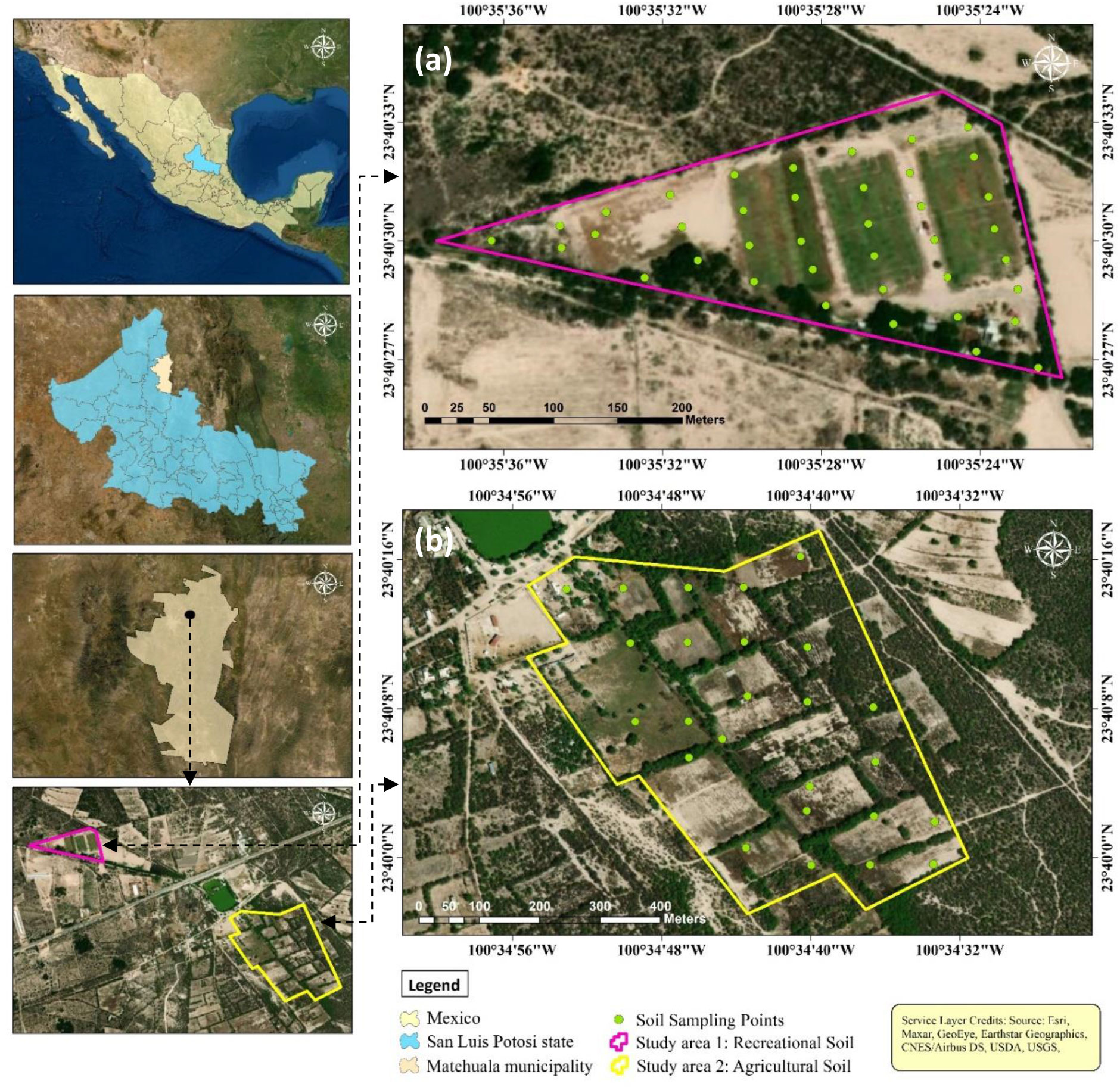
Figure 1 Study area map showing metal concentrated soil sampling locations of (A) recreational soil and (B) agricultural soil.

3. Materials and methods

3.1. Sampling of soil and chemical analysis

A total of 64 surface soil samples (from 0 to 5 cm) were collected from both recreational and agricultural areas, of which 39 samples were from recreational soil sites (study area 1) and 25 samples were collected from agricultural soil sites (study area 2). A depth from 0 to 5 cm is appropriate and mandatory in the Mexican regulations and recommendations for trace metal and metalloid identification and quantification to characterize potentially contaminated soils (71). In this study, a systematic sampling technique was used based on a statistical method (NMX-132-SCFI-2001) (71). These samples were taken with an auger and stainless steel shovel to prevent contamination and cleared of roots and rocks larger than 2 cm, before being placed in a double polyethylene bag. Over the study area, soil samples were distributed uniformly, with an average of 40-50 m for recreational soil area and 80-100 m for agricultural soil area between each sampling point. The agricultural land in the sampling site had calcareous alluvium overlying soil with high gypsum content. During the sampling campaign, the study teams faced a few problems in collecting equidistant samples, such as, consent from the owner of the farm, eroded topsoil, with exposed gypsisol soil, and various forms of obstruction. For the same reason, samples are fewer than the recreational soil. Despite such constraints, a significant number of samples were collected. As a standard procedure, a typical soil sample of 1 kg of fresh surface soil was collected from each sampling site and wrapped in a sealed double polyethylene bag before delivering to the testing centre (22, 67). All soil sampling sites were georeferenced using a GPS tracking device called a Garmin Etrex Personal Navigator. According to a slightly modified version of ISO 11466:1995, soil samples were digested for chemical analysis. For doing so, 10 mL of aqua regia (HNO₃:HCl) with a ratio of 3:1, were added to a beaker containing 1.0 gm of soil sample (20, 67). The beakers were heated to 85°C until the digests had nearly dried out. The resolved residues were added to volumetric flasks, allowed to cool, and then filtered through Whatman filter paper no. 40 before being redissolved in 10 mL of acid and made up to 50 mL with 0.5 M nitric acid. All digested and diluted samples were refrigerated at 4°C for analyses (20, 67). After further diluting with deionized water, aliquots of the digested samples were analysed for As, Ca, Mg, Na, K, Sr, Mn, and Fe by using inductively coupled plasma optical emission spectroscopy (ICP-OES) (67, 72).

3.2. GIS interpolation techniques for spatial distribution mapping

When it is unfeasible, inconvenient, or costly to explore each site within the selected study region, an interpolation technique is applied to estimate unknown parameters for geospatial factors like elevation, slope, concentration levels, rainfall, temperature, and noise levels with a limited range of collected data points (73, 74). For assessing the spatial distribution of contaminants in soils, inverse distance weighting (IDW) is a frequently used interpolation technique because of its easy calculation and convenient data analysis approach (37, 75, 76). The IDW is a type of deterministic interpolation technique that works for data points that are close to one another than distant points. The spatial variability of the metal concentration levels and source distribution factors was simplified using the IDW approach with a weighting power of 2 (19, 37). The distance between the estimated and observed sampling points, increased to the power values has a substantial impact on the weights. The impact of the distant points decreases with an increase in power while weights are distributed across adjacent points more evenly for lower power (77, 78). For this interpolation approach, the following formula is used.

$\begin{array}{ll}\text{Z}={\displaystyle \sum _{i=1}^n(Z_i/d_i^p)}/{\displaystyle \sum _{i=1}^n(1/d_i^p)}& (1)\end{array}$

Where Z is the projected value at an interpolated point, Z_i is the measured value at point i ; n denotes the total amount of measured values used for interpolation; d_i is the distance between interpolated value Z and measured value Z_i ; p indicates the weighting power, which specifies how the weight reduces as the distance rises. A methodological flowchart that illustrates how soil samples are obtained and subsequent methods for identifying the sources of toxic elements in the surface soil are shown in Figure 2.

FIGURE 2

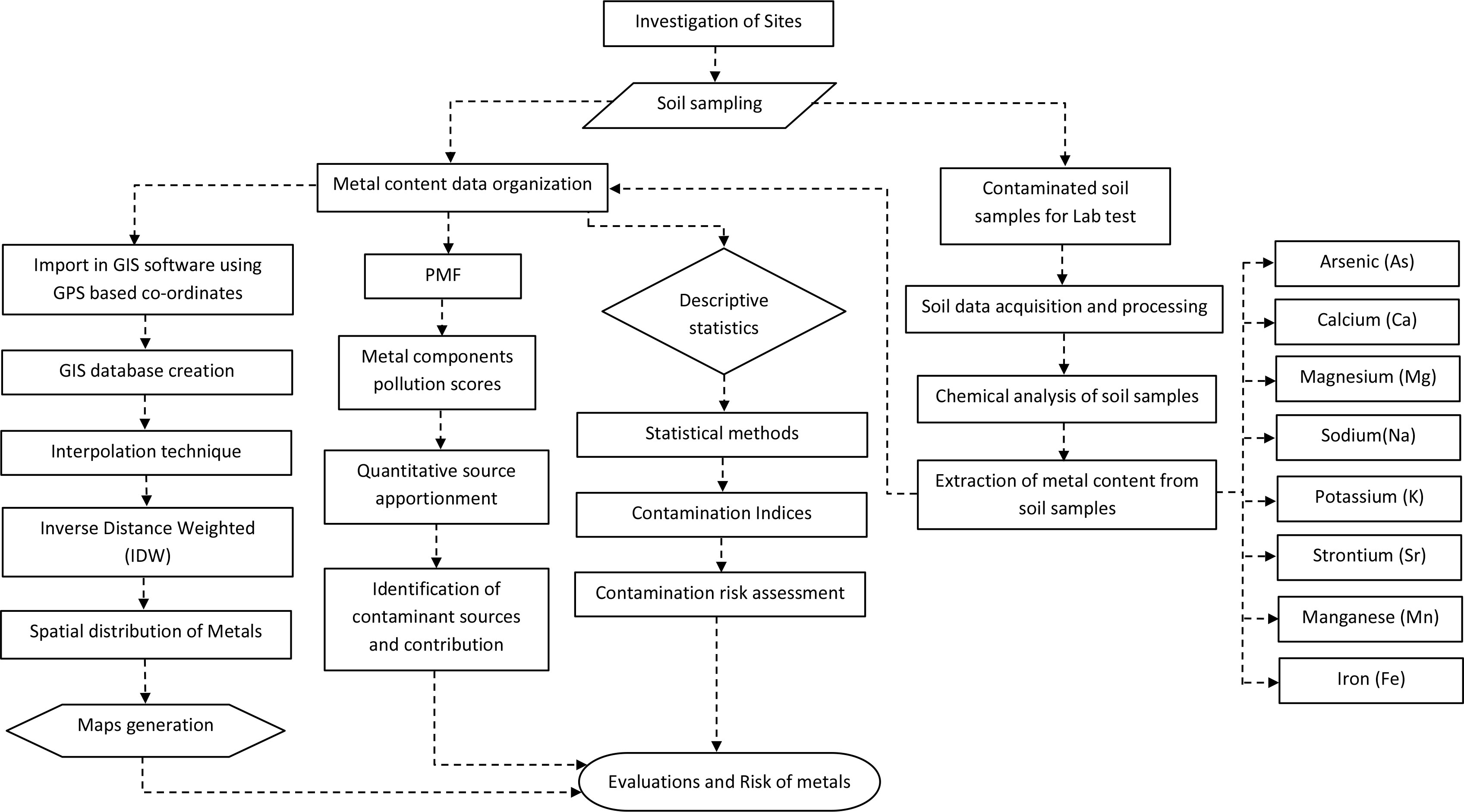
Figure 2 Flowchart illustrating the methodology of this study.

3.3. Risk assessments of metal contamination based on indices

3.3.1. Geo-accumulation index

The geo-accumulation index (I_geo) has been widely used as a biogeochemical criterion to assess the contamination level of a specific metal in environmental soil or sediments since 1969 (44, 79). This index (I_geo) was developed by Muller (80) to determine the contamination level of toxic metal concentration in soil by comparing the total metal components measured to its reference level or background value of concentrations. To assess the level of metal pollution in the soil, I_geo is calculated using the following equation:

$\begin{array}{ll}{I}_{geo}={\log }_2\frac{C_n}{1.5 B_n}& (2)\end{array}$

Where, C_n is the observed metal concentration in the soil sample (mg/kg), B_n indicates the background reference value for n metal in the soil (mg/kg), and the constant factor 1.5 was used to adjust the background matrix for any differences induced by lithospheric influences (44). Table 1 shows the seven different classifications of I_geo according to the contamination levels.

TABLE 1

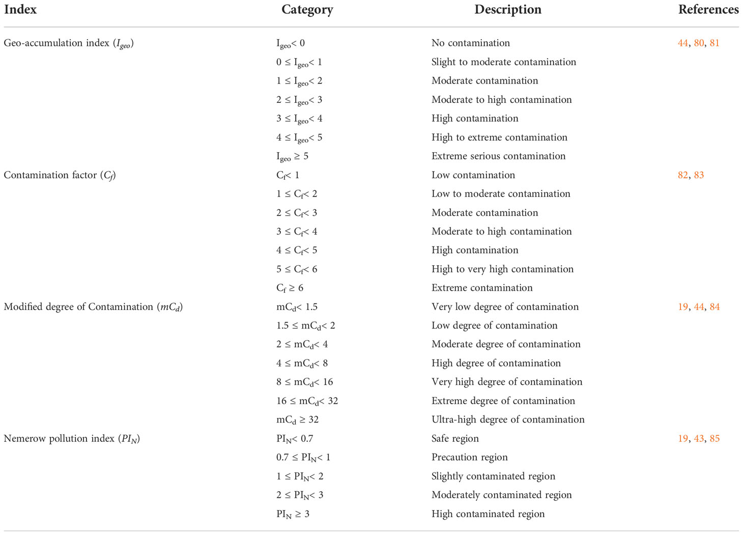
Table 1 Contamination indices based on the classification of soil.

3.3.2. Contamination factor

The contamination factor (C_f) index is considered to be a valuable approach for detecting and identifying hazardous metal contamination over time (86, 87). In order to estimate the amount of contamination for specific metals, the contamination factor is commonly implemented, and it is specified as the proportion of the metal concentration to the mean of background reference level concentrations. This index is also known as the single pollution index (82). The contamination factor (C_f) is determined using the following equation:

$\begin{array}{ll}{C}_f=\frac{C_m}{C_b}& (3)\end{array}$

Where, C_m denotes the observed metal concentration in the soil sample and C_b is the background reference level concentration of the selected metal. The contamination factor (C_f) is divided into seven classes, as indicated in Table 1.

3.3.3. Modified degree of contamination

The modified degree of contamination (mC_d) is the ratio of the sum of the contamination factor of each selected metal to the total number of measured metals in the soil, which is used to calculate the absolute degree of contamination in a specific soil sample (88). The mC_d computation includes the inherent characteristic of providing an average total value for a variety of contaminants (89). The following equation is a modified generalised approach to calculating the degree of contamination:

$\begin{array}{ll}m{C}_d=\frac{{\displaystyle {\sum }_{i=1}^n{C}_f}}{n}& (4)\end{array}$

Where, C_f refers to the contamination factor, i is the i th metal or selected specific metal in the soil sample, and the total number of metals in the soil sample is denoted by n . The modified degree of contamination (mC_d) is divided into seven different classes, as indicated in Table 1.

3.3.4. Nemerow pollution index

The Nemerow Pollution Index (PI_N) is a technique for measuring the comprehensive level of contamination in the surface soil based on contamination factors, and it comprises metal concentration assessments (19, 85, 90). This approach may offer a logical explanation of the heavy metal contamination at each site in its entirety because many contaminants can affect a specific site (91). The following equation is used to compute PI_N:

$\begin{array}{ll}P{I}_N=\sqrt{\frac{{(C{f}_{max})}^2+{(C{f}_{average})}^2}{2}}& (5)\end{array}$

Where, Cf_max is the highest contamination factor value of each metal in the soil samples and Cf_average is the average contamination factor value of all the collected soil samples for each specific metal. The five different classes of metal contamination in soil are shown in Table 1 based on PI_N values.

3.4. Positive matrix factorization model analysis

The PMF receptor model 5.0, which was developed by the US Environmental Protection Agency, was used to identify, and distribute the pollution sources of contaminants (92). Paatero and Tapper (93) introduced the improved factorization technique known as PMF in the early 1990s (50). The PMF is the statistical technique for determining the contribution of sources to sample datasets depending on the patterns of the sources. The identification and classification outcomes of the PMF model offer significant advantages compared with other approaches, such as principal component analysis (PCA) (94). The purpose of this model is to factorise the initial matrix X (i x j) into two-factor computational matrices F (k x j) and G (i x k), and an additional residual matrix E (i x j). The fundamental PMF formula is as follows:

$\begin{array}{ll}{X}_{ij}={\displaystyle \sum _{k=1}^p(G_{ik}\times F_{kj})}+E_{ij}& (6)\end{array}$

Where, X_ij represents the concentration amount of j^th metal observed at the i^th sampling point, G_ik denotes the contribution of the k^th source to i^th sample, F_kj represents the concentration amount of j^th metal from the k^th source, E_ij denotes the residual error matrix, and p indicates the individual sources. The PMF model uses uncertainty in data quality to normalise each element’s prediction error in matrix X. It generates the optimal concentration matrices, G and F, within non-negative ranges that minimise the objective function Q (61). The calculation of Q is as follows:

$\begin{array}{ll}Q={\displaystyle \sum _{i=1}^n{\displaystyle \sum _{j=1}^m\left(\frac{X_{ij}-{\displaystyle {\sum }_{k=1}^p{G}_{ik}\times F_{kj}}}{U_{ij}}\right)}}={\displaystyle \sum _{i=1}^n{\displaystyle \sum _{j=1}^m{\left(\frac{E_{ij}}{U_{ij}}\right)}^2}}& (7)\end{array}$

Where U_ij denotes the uncertainty in the j^th metal for the i^th sample, E_ij indicates the residual error matrix, m refers to the number of metals, and n is the number of samples. The data regarding concentration and uncertainty are necessary for the PMF model. The uncertainty in the Method Detection Limit (MDL) of a specific metal uses its concentration and specified error fraction. If the MDL value is exceeded by the metal concentration, the following formula can be used to determine the uncertainty:

$\begin{array}{ll}{U}_{ij}=\sqrt{{(\sigma \times c)}^2+{(MDL)}^2}& (8)\end{array}$

Where, σ denotes the relative standard deviation of each metal or error fraction and c represents the concentration of metals.

Otherwise, the uncertainty is calculated using the following equation:

$\begin{array}{ll}{U}_{ij}=\frac{5}{6}\times MDL& (9)\end{array}$

The value of the method detection limit (MDL) is calculated as follows (95):

$\begin{array}{ll}MDL=t_{(n=1, 1-\propto =0.99)}{S}_s& (10)\end{array}$

Where, t_{(n=1, 1−∝=0.99)} represents the Student’s t-value, appropriate for a single-tailed 99th percentile t statistic and a standard deviation estimate with n-1 degrees of freedom, and S_s is the sample standard deviation of the replicate spiked sample analyses.

The Bootstrap (BS) approach was used to evaluate the PMF results’ uncertainties and included random errors which reflect variability in the samples, or the disproportionally effect of the observations on the PMF result (37, 96). The uncertainties might be represented by the mean uncertainty, which is the range between the concentration of the base factor and the upper uncertainty limits for the BS. The USEPA PMF 5.0 User Guide (the 92) is followed for all calculations.

3.5. GIS and statistical analysis

The statistical analyses were performed on the data using the SPSS v28.0 statistical package (IBM Inc., USA) and Microsoft Excel 2016 to identify the statistical descriptions of metals in surface soil samples. The observed data were initially assessed using the Kolmogorov-Smirnov test to confirm the normal distribution. The one-way analysis of variance (ANOVA) was performed to assess if there was a statistically significant difference between the means of the different sampling points. The spatial distributions were characterised using a deterministic model and the IDW interpolation technique. The distribution of soil sampling locations and the spatial distribution of metals were analysed and mapped using ArcGIS Pro (ESRI Inc., USA). The PMF model was implemented and the source of the metals in this study was quantitatively identified using the EPA PMF 5.0 software (92).

4. Results and discussion

4.1. Descriptive statistics of metal concentrations in soil

The statistical information of the metal concentrations in surface soil samples is summarized in Table 2. The mean concentrations of As, Ca, Mg, Na, K, Sr, Mn, and Fe in recreational soil were 119.44 mg/kg, 20346.45 mg/kg, 1195.53 mg/kg, 1397.06 mg/kg, 3358.07 mg/kg, 514.10 mg/kg, 137.82 mg/kg, and 3700.52 mg/kg. The mean values of metal concentrations in the agricultural soil were 76.90 mg/kg, 28975.41 mg/kg, 2838.28 mg/kg, 188.78 mg/kg, 5420.28 mg/kg, 352.66 mg/kg, 275.27 mg/kg, and 6933.74 mg/kg, respectively. Overall, in both study areas’ soil, the mean value of metal concentrations exceeded the corresponding permissible limits or reference values for soils, except Na metal. The permissible limits or reference values of metal concentrations in the surface soil were As (22 mg/kg) (97), Ca (500 mg/kg) (98), Mg (60 mg/kg) (98), Na (1550 mg/kg) (98), K (300 mg/kg) (98), Sr (200 mg/kg) (99), Mn (85 mg/kg) (100), and Fe (300 mg/kg) (101). The mean concentrations of As, Ca, Mg, K, Sr, Mn, and Fe were higher than the reference values in the recreational soil by approximately 5.43, 40.69, 19.93, 11.19, 2.57, 1.62, and 12.34 times. And, for the agricultural soil by approximately 3.50, 57.95, 47.30, 18.07, 1.76, 3.24, and 23.11 times, respectively. Compared with the permissible limit values defined by the various researchers for soils, the mean concentrations of heavy metals like As, Sr, Mn, and Fe were all higher than the severe risk screening levels, revealing that the soil poses a health risk for agricultural and recreational uses.

However, the concentration of As in recreational and agricultural soil was around 5.43 and 3.50 times greater than the permissible limit, revealing that As was enhanced in the topsoil through metallurgical activities, irrigated groundwater, and human activities. In addition, there is a major concern for As in Mexican soils with rigorous monitoring in place to restrict potential contamination. The ratio of standard deviation to mean is known as the coefficient of variation (CV), and it can be used to analyse the distribution of metal concentrations in the soil as well as their variability (102). According to the study of Wilding (103), the coefficient of variation is classified into three different levels: low (CV< 0.16), medium (0.16< CV< 0.36), and high (CV > 0.36). The coefficient of variation (CV) of Na in the surface soil of both study areas was the highest (280.20%). However, the CVs of As in the recreational and agricultural topsoil recorded a high variation, 91.71%, and 50.05%, respectively. The CVs of metals in the recreational soil were in the following increasing order: Na (280.20%)< As (91.71%)< Mg (49.67%)< Sr (48.49%)< Ca (35.99%)< Fe (35.32%)< K (29.72%)< Mn (29.60%). Overall, the degree of variation for metals is high for the recreational soil, except for K and Mn, which are in the medium range. The same as the CVs of metals in the agricultural soil were in the following increasing order: As (50.05%)< Na (47.42%)< Sr (36.56%)< Fe (14.36%)< K (14.27%)< Mn (12.55%)< Mg (9.47%)< Ca (4.29%). The findings (Table 2) showed that CVs of As, Na, and Sr indicated a high variability, while those for Fe, K, Mn, Mg, and Ca indicated low variability. Previous studies showed that human influences have a significant impact on the concentration of metals when the mean concentration value of metals in the surface soil is higher than the reference value and the CV is more than 0.2 (102, 104). Overall, there was more variation and spatial dispersion in the concentration of metals in the recreational soil of the study region than in agricultural soil, and it is expected that anthropogenic activities have an impact on this concentration.

TABLE 2

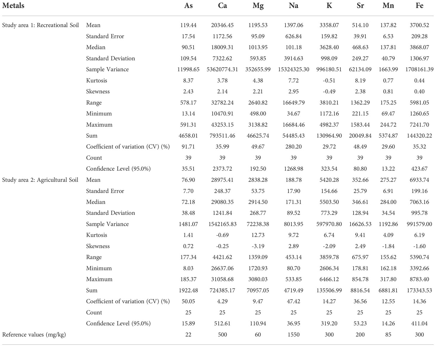
Table 2 Descriptive statistics of metal concentrations for soil physicochemical properties.

4.2. Spatial distributions of metal concentrations in soils

Finding contaminated regions with high metal concentrations and identifying their potential sources can be accomplished by analysing the spatial distribution approach of metal concentration. The spatial distributions of As, Ca, Mg, Na, K, Sr, Mn, and Fe were used to identify the distribution pattern of metals in two study locations. Based on the spatial distribution of metals, the polluted regions with high metal concentrations were mostly found in both study areas and were comparable to recreational and agricultural soil. In order to evaluate the risk assessment and contamination hotspots, Figures 3, 4 show the spatial distribution of the eight selected metals using the IDW interpolation technique. It is considered that the assumptions are quite a linear combination of the accessible data when using the inverse distance weighting (IDW) interpolation technique (50). According to Figures 3, 4, point source contamination can be inferred from the concentrations of As, which were spatially distributed as being relatively high. The highly contaminated areas containing Ca, Mg, K, Sr, Mn, and Fe were found in the south-western part of the recreational soil study area. The spatial distribution of Ca, Mg, Sr, and Fe were similar, and the high-value areas of all metals were quite extensive. The distribution pattern of metals in agricultural soil was clear through spatial analysis. Similar to the recreational soils, the agricultural soil contained higher levels of Ca, Mg, K, Sr, Mn, and Fe, with the highest values located in the northern to southern parts of this area. Mg in the agricultural soil was mainly in the south and south-eastern parts of the study area. The areas with the highest As and Sr values were alongside narrow roads and the waterbody and were mostly in the north-western part. As and Sr had comparable spatial variation features. The As concentration hotspots in both study areas were mainly associated with irrigated groundwater and past mining activities. The significantly related distinction of the parent material during soil formation and other anthropogenic activities may be the reason for the high concentrations of other metals (except Na) in these regions. This indicated that climatic effects like wind and rainfall events may potentially affect the distribution of metals in the area of study. Since the climatic environment in the study areas is semi-arid having limited precipitation, irrigated cultivation is the preferred mode of agriculture. Due to this reason, the concentration levels of heavy metals like As, Mg, Sr, and Fe are high in these study areas. As a result, it may be stated that the study areas’ climate has some impact on the spatial distribution of metal contaminations. On the whole, the metal distribution in both recreational soils and agricultural soils showed similar distribution patterns. Moreover, the high-value range of all metal concentrations exceeded the permissible limits or the reference values, and the cause may be connected to the metallurgic and natural origin of metals, past mining industry, groundwater irrigation, and intense human activities.

FIGURE 3

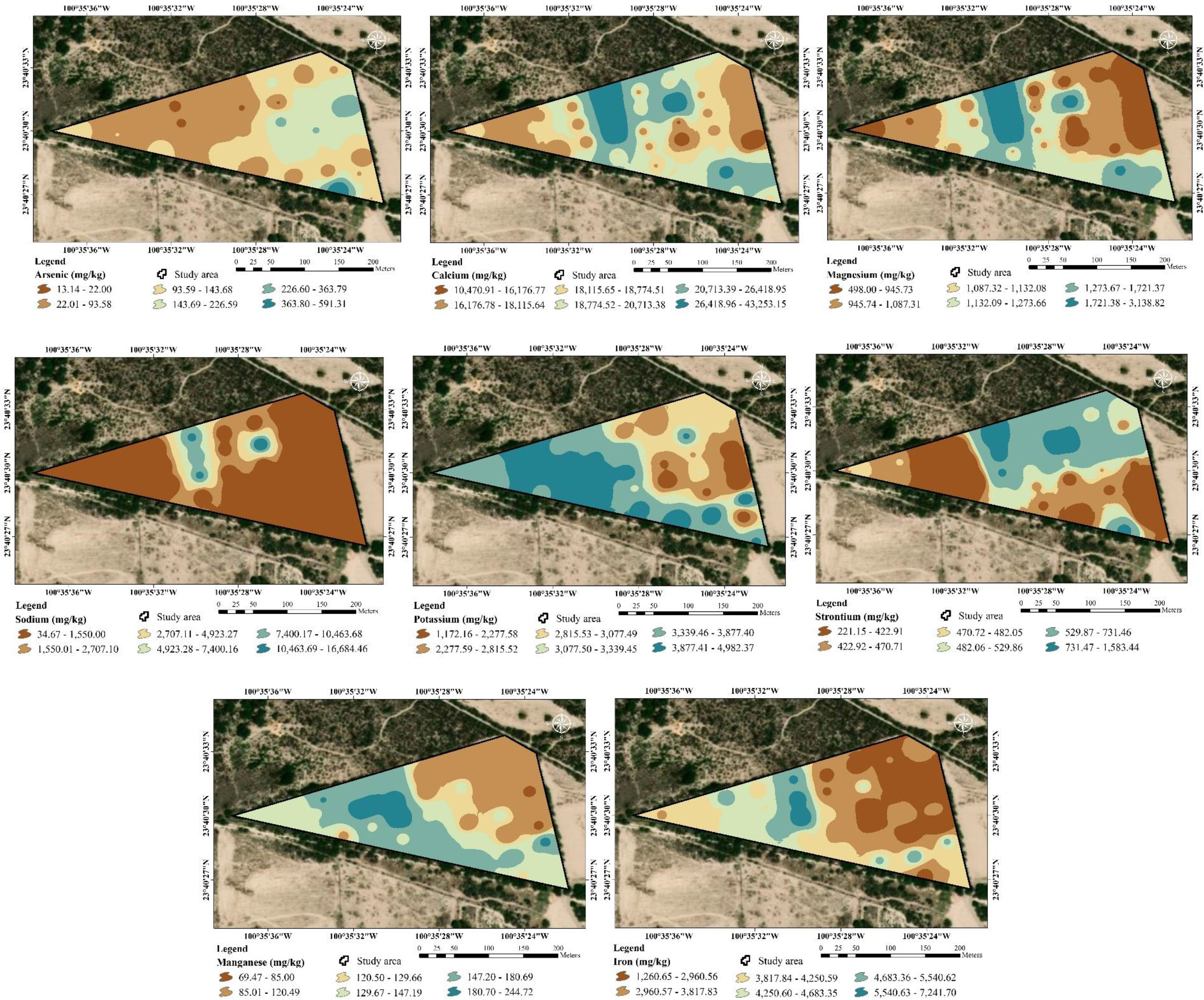
Figure 3 Spatial distribution of metal concentrations in the recreational soil.

FIGURE 4

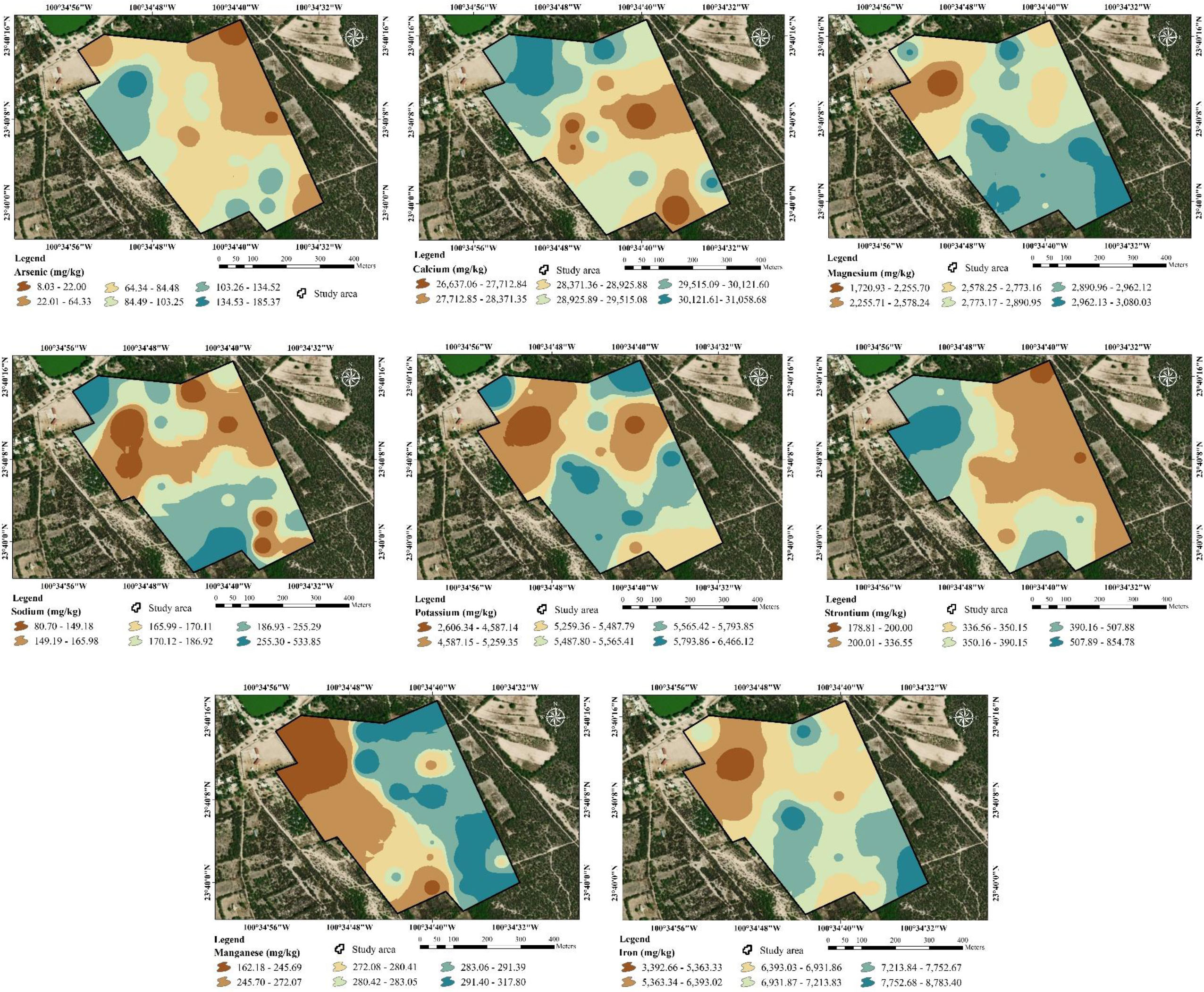
Figure 4 Spatial distribution of metal concentrations in the agricultural soil.

4.3. Contamination risk assessments in soils

The I_geo analysis was utilised to determine the extent of cumulative concentration of metals in the soil along with the amount of heavy metal contamination. Figure 5 shows the box plot diagram of metal contamination assessment based on I_geo index for both recreational and agricultural soil. The descriptive analysis of contamination risk assessment by different types of contamination indices is shown in Table 3.

FIGURE 5

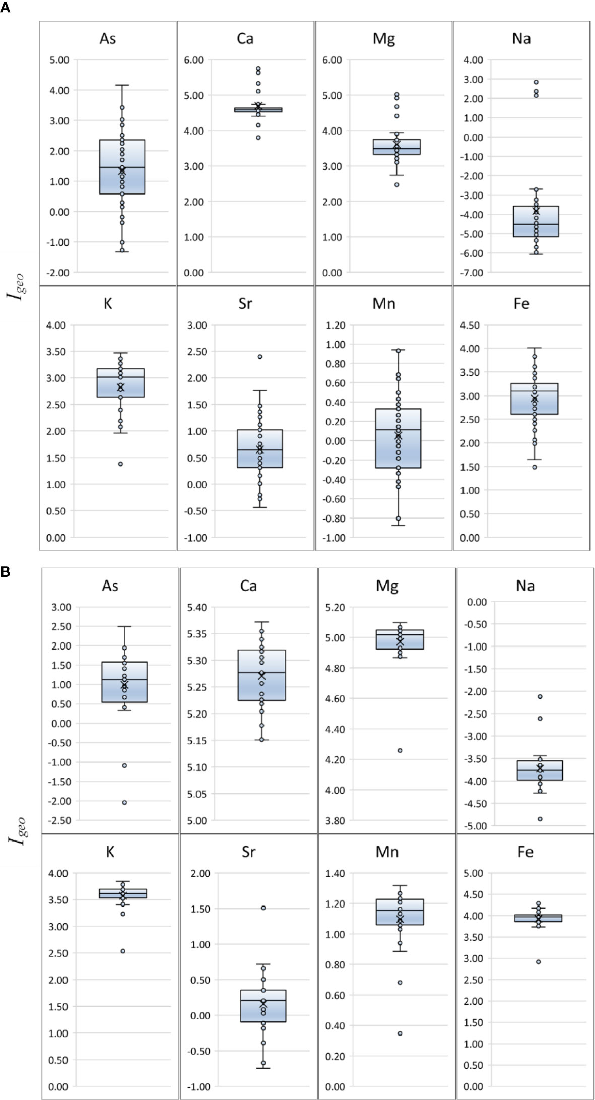
Figure 5 Box plot of metal contamination assessment based on Geo-accumulation index (I_geo) for (A) recreational soil and (B) agricultural soil.

TABLE 3

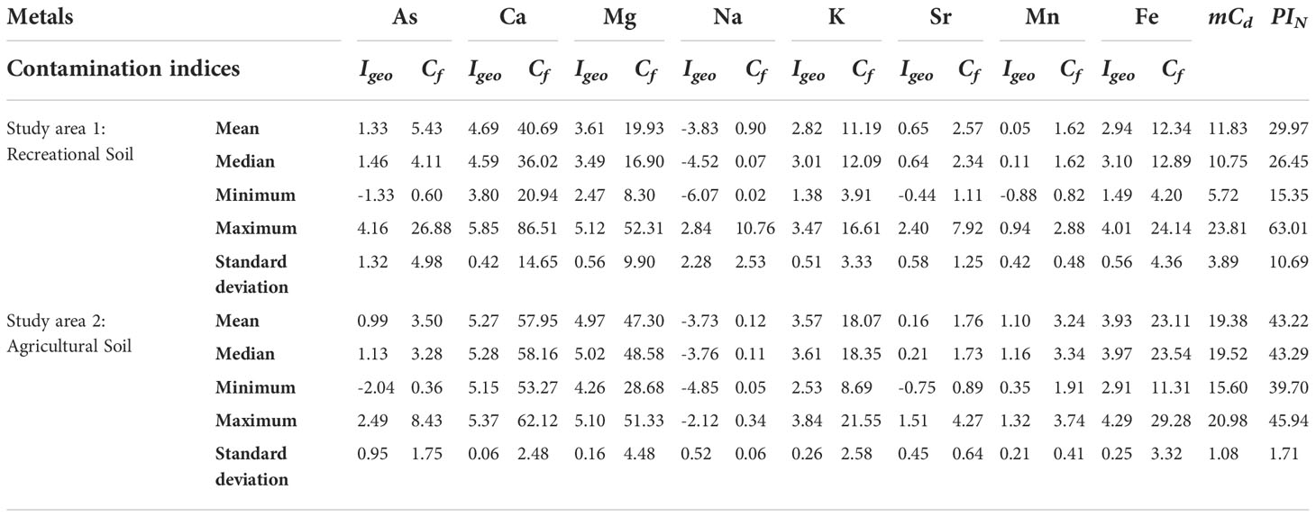
Table 3 The metal contamination and risk assessment by different types of contamination indices.

The mean I_geo index values of metals in recreational soil were arranged in the decreasing order of Ca (4.69)> Na (3.83)> Mg (3.61)> Fe (2.94)> K (2.82)> As (1.33)> Sr (0.65)> Mn (0.05), while the mean I_geo values of metals in the agricultural soil were in the following increasing order of Ca (5.27)> Mg (4.97)> Fe (3.93)> Na (3.73)> K (3.57)> Mn (1.10)> As (0.99)> Sr (0.16). The mean I_geovalues of all metals were greater than zero, indicating that all metals contributed to pollution in the surface soil in both study areas and more than 90% of the soil samples were at polluted levels. In the recreational soil, the mean I_geo values of Ca, Na, and Mg were greater than 3, indicating a polluted condition. The mean I_geo values of Ca, Mg, Fe, Na, and K in the agricultural soil were also more than 3, suggesting contamination. Equally, the study area had high contamination levels of heavy metals like As, Sr, Mn, and Fe.

The computation of the contamination factor assessment for each metal is shown in Figure 6, and the classification criterion for the contamination factor index is listed in Table 3. The mean values of C_f of each metal in the recreational soil were ranked in the decreasing order of Ca> Mg> Fe> K> As> Sr> Mn> Na, with values of 40.69, 19.93, 12.34, 11.19, 5.43, 2.57, 1.62, and 0.90. And for the agricultural soil, the mean values of C_f were ranked in the following decreasing order of Ca> Mg> Fe> K> As> Mn> Sr> Na, with values of 57.95, 47.30, 23.11, 18.07, 3.50, 3.24, 1.76, and 0.12, respectively. The C_f values for As in the recreational soils showed a ‘high to very high contamination’ category, while the C_f values for As in the agricultural soils indicated moderate to high contamination. More than 30% of soil samples of As are in the extremely high level in the recreational soil, while less than 10% of the agricultural soil samples are in the extreme contamination level (Figure 6). Hence, it can be concluded that As contaminants are at a higher level in recreational soil than in agricultural soil. The other heavy metals like Sr, Mn, and Fe fluctuate at low to high levels of contamination in both study soils.

FIGURE 6

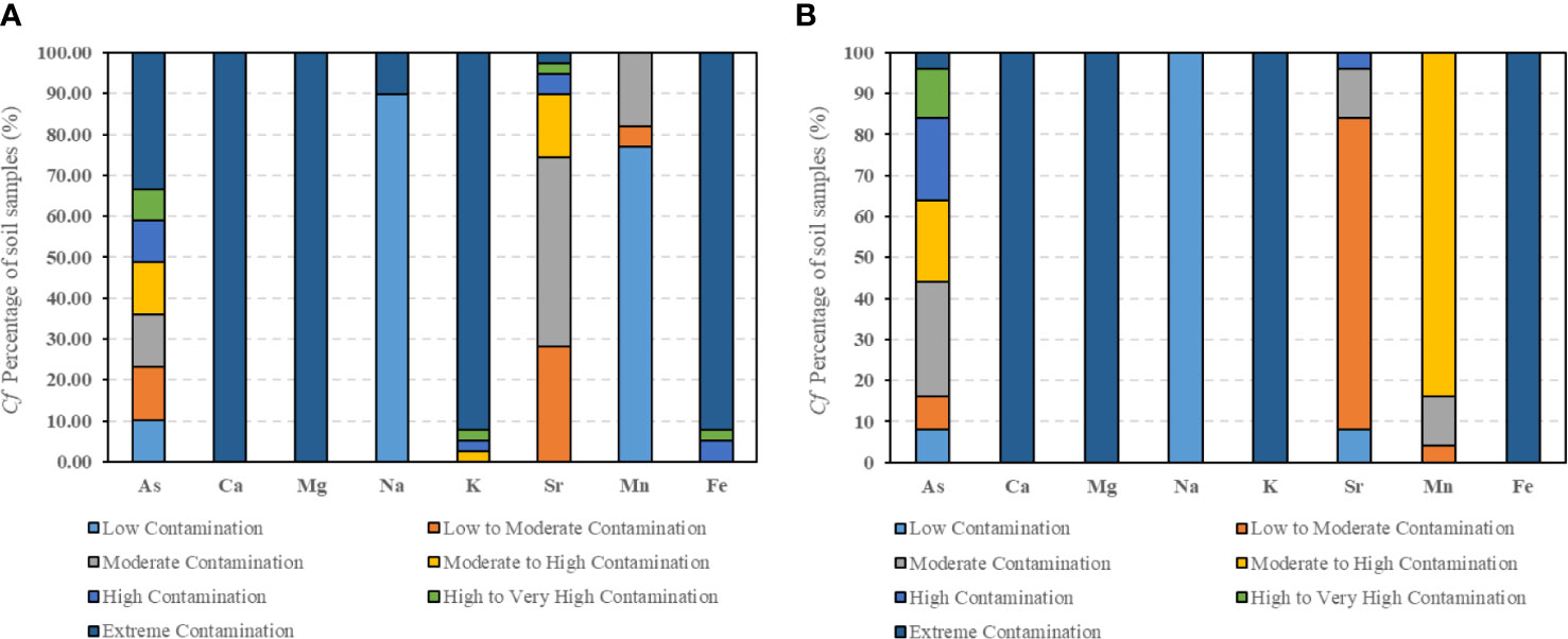
Figure 6 Contamination factor (C_f) percentage of metals for (A) recreational soil and (B) agricultural soil at different contamination level.

Figure 6A showed that the levels of contamination were extremely high for all recreational soil samples of Ca and Mg. And Figure 6B shows that all agricultural soil samples of Ca, Mg, K, and Fe had high levels of contamination. Overall, the mean modified degree of contamination (mC_d) computed for the recreational and agricultural soils was 11.83 and 19.38, respectively. These values indicate that the recreational soils have a very high contamination level while the agricultural soils have an extremely high degree of contamination level. When Nemerow Pollution Index (PI_N) > 3, metal contamination in soil is considered to be high. However, the mean PI_N values for surface soil in the study areas of recreational and agricultural soils were 29.97 and 43.22, respectively, showing that the majority of the soil samples in both soil areas were extremely polluted by metals. However, reports of As pollution and risk for the recreational soil and agricultural soil area have already been published previously (19, 20, 67). The highly contaminated and precautionary stages were observed in both study areas, due to past metalliferous mining and anthropogenic activities. Therefore, it was possible to conclude that the soil in the abandoned metallurgical region had been severely contaminated. And the level of pollution is increasing because of natural soil formation, the use of contaminated groundwater for irrigation, and human activities. It was suggested that specific environmental restoration should be carried out.

4.4. Source apportionment of metals using PMF

The identification of sources and apportionment of metals in the soils were further determined using the PMF model. The model’s starting parameters included 3, 4, and 5 factors, a start seed number chosen at random from 20 iterations. The lowest and most reliable Q true value was used to calculate the ideal number of factors (4, 61). To regulate the residual matrix E, the minimum Q must be found, after which one can determine an acceptable number of factors (105). The least Q value was obtained from the optimum output of the PMF model, which included four factors. The predicted residuals of most soil samples were normally distributed within a range of -4 and 4. The past mining activities as well as industrialization, natural soil formation, groundwater sources, and human activities were identified as the four main sources of metal pollution. Sources were not identified based on one characteristic of a factor but also using the process of evidence by conflict, which involved additional factors. In general, the mean metal concentration values were initially used to determine whether the major sources of the metal contamination were natural or anthropogenic. The relationship between observed and predicted metal concentrations for the recreational and agricultural soil is shown in Figures S1, S2. The R² values of selected metals in recreational soil (Figure S1) were as follows after model fitting: As (0.99), Ca (0.90), Mg (0.94), Na (0.99), K (0.79), Sr (0.99), Mn (0.83), and Fe (0.95); and for the agricultural soil (Figure S2) were as follows: As (0.99), Ca (0.40), Mg (0.94), Na (0.99), K (0.81), Sr (0.99), Mn (0.75), and Fe (0.84). All of these models generated R² values of more than 0.7, indicating a significant correlation between selected metals and the utilisation of a sufficient number of factors obtained from the PMF model.

4.4.1. Identification of source factorization to recreational soil

The results of the source contribution and factorization of metal concentration in recreational soil by PMF analysis are shown in Figure 7. The geographical interpolation method produced the spatial distribution characteristics of four factors. Figure 8 shows four factors whose spatial distribution patterns were formed using the deterministic IDW interpolation approach and which indicated significant spatial correlation with strong outputs. The source profiles in mg/kg and source contribution rates in percentages (%) of each factor to the metals using the PMF model are shown in Table 4.

FIGURE 7

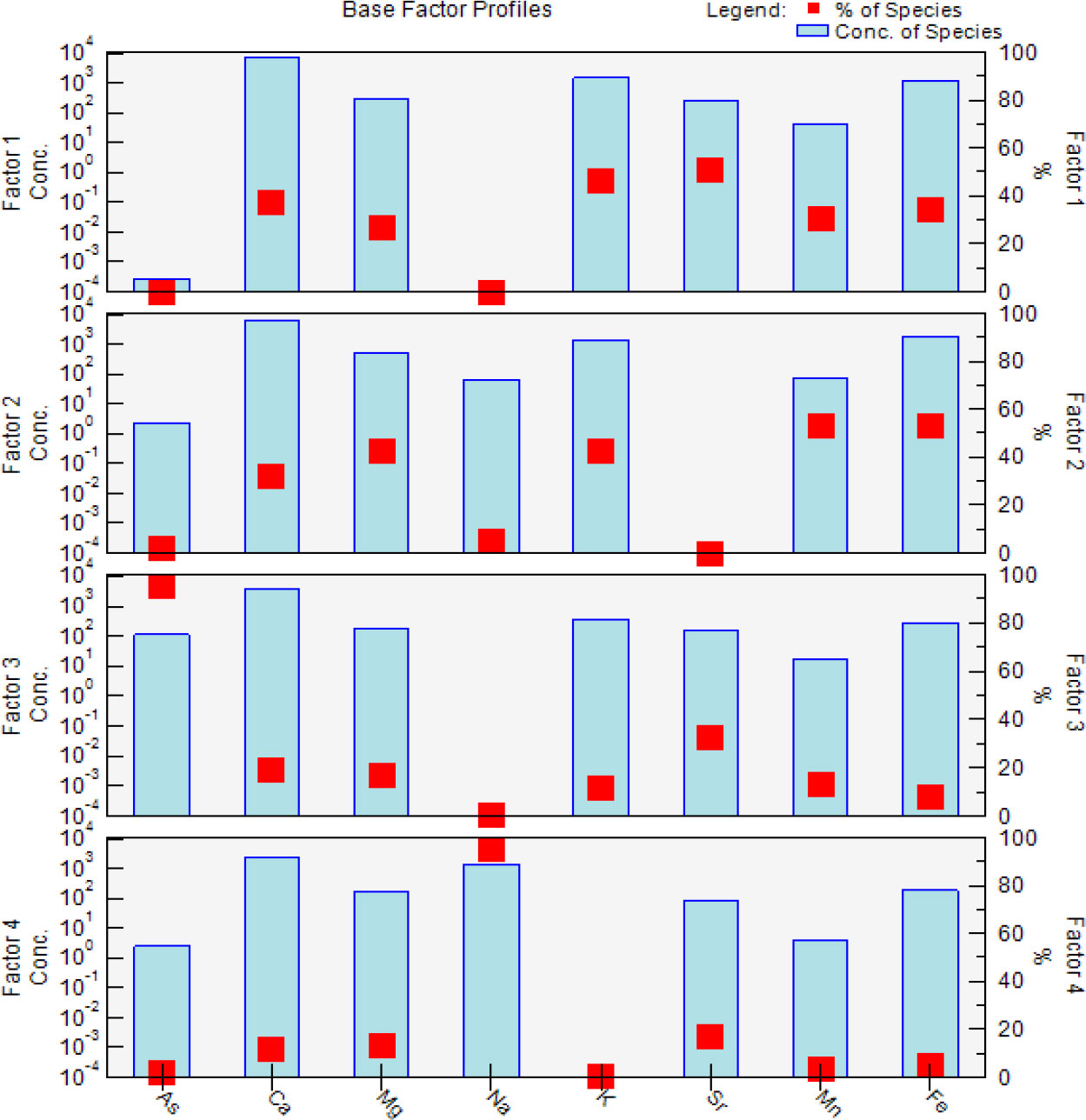
Figure 7 Factor profiles and source contributions of metal concentrations from PMF for recreational soil.

FIGURE 8

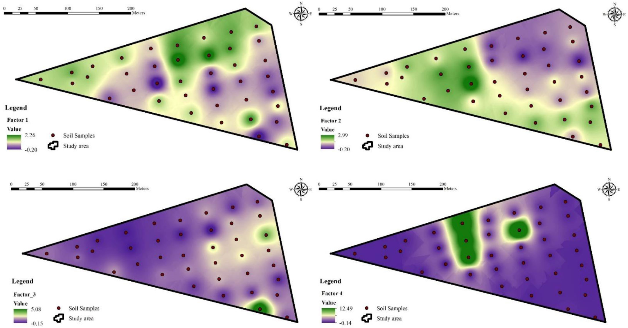
Figure 8 Spatial variations for the normalization from each of the four factors within the recreational soil.

TABLE 4

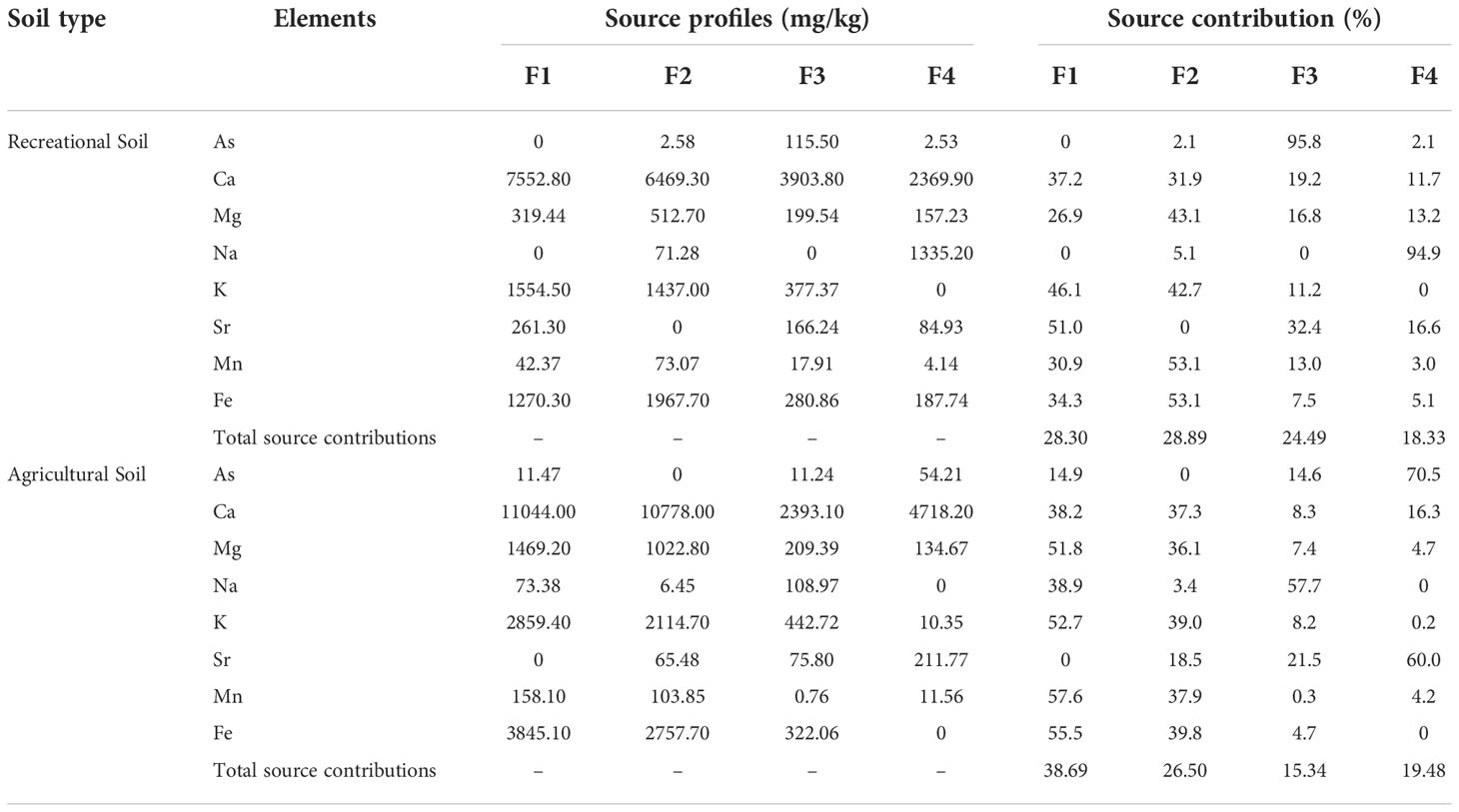
Table 4 Source contribution rates of factors for metal concentrations in the soil.

Factor 1 was mostly affected by K and Sr with source profiles of 1554.50 mg/kg and 261.30 mg.kg^-1, and the contribution rate of 46.1% and 51%, respectively (Table 4). It also contributed 37.2% and 34.3% to Ca and Fe in this factor. The areas with high-level factor 1 values were found in minor quantities at scattered locations. Soil-Sr concentration is typically considered to be a key factor for the deposition of air dust particles that have interacted with strontium ions from industrial operations and may potentially be exacerbated by human activity. The reason behind the increase in K levels in this area were includes the tillage system, soil temperature, soil permeability, oxygen content, and soil moisture. The higher soil moisture often results in more K being generated. As a result, factor 1 could mostly be considered to involve natural activities.

Factor 2 provided an explanation for the high loadings of Mn (53.1%), Fe (53.1%), Mg (43.1%), and K (42.7%) (Table 4). Mn and Fe are widely found at higher acidic levels in soils, increasing alkalinity levels. Metal casting, soil formation by chemical processes, and other industrial activities all have the potential to produce Mg and K in the environment (106). As a result, factor 2 possibly reflected past mining and industrialization activity sources.

Factor 3 described the significant loadings of heavy metals like As (95.8%) and Sr (32.4%) (Table 4). Possible sources of Sr bonded to As include paedogenic processes, mining and ore processing operations, As-contaminated groundwater, and waste disposal. But previous studies have shown that arsenic levels in these soils are elevated only for the As-contaminated irrigated groundwater. Studies conducted in the past revealed that the groundwater in the study area contained exceptionally high levels of As, which came from the dissolution of metallurgical wastes from an abandoned smelter upstream, near Matehuala (18, 19, 67). Here, the soccer fields are maintained by irrigation using groundwater. Hence, the contaminated groundwater might be interpreted as factor 3.

Factor 4 was mainly contributed by Na with source contribution amount and rate of 1335.20 mg/kg and 94.9%, respectively (Table 4). In the study, Na was the only metal with concentrations below permissible levels. The high-value locations of factor 4 and soil-Na concentration were mainly distributed in the middle of the study area which refers to the soccer pitch (Figure 8). The majority of Na concentration in soil was from pesticides, fertilizers, and other human activity. Therefore, factor 4 may represent anthropogenic activities such as different types of human activities.

4.4.2. Identification of source factorization to agricultural soil

The schematic of the factor profiles and source contributions percentages for various metals in agricultural soil based on PMF results is shown in Figure 9. Table 4 depicts the parameters for the PMF modelling with four factors of sources. The spatial distribution mapping of source contributions determined by the PMF results was assessed using the IDW interpolation technique, shown in Figure 10.

FIGURE 9

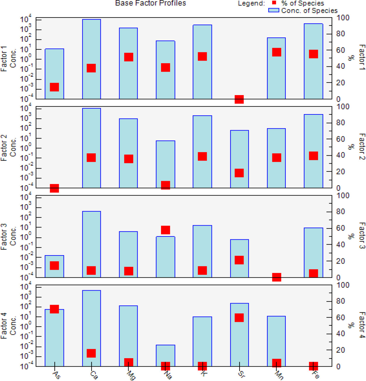
Figure 9 Factor profiles and source contributions of metal concentrations from PMF for agricultural soil.

FIGURE 10

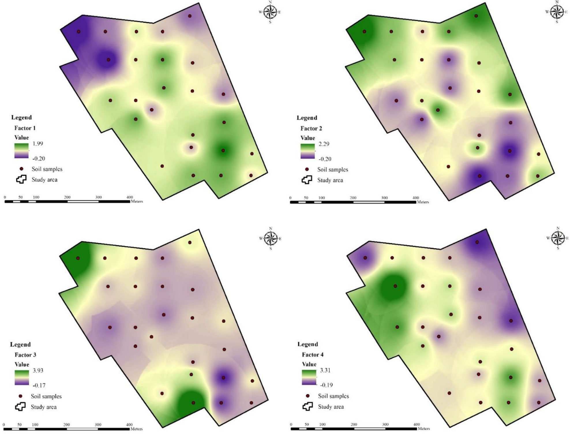
Figure 10 Spatial variations for the normalization from each of the four factors within the agricultural soil.

Factor 1 revealed the specific representation of the factor profiles and source contribution of each metal using the PMF model, which shows Mg (51.8%), K (52.7%), Mn (57.6%), and Fe (55.5%) having high factor loadings than the other metals (Table 4). According to the spatial distribution map of factor 1, the high-value locations are clustered around the agricultural land and the south-eastern part (Figure 10). The soils in the study area were severely polluted by heavy metals like Mn and Fe and indicating substantial mining activities and industrialization impacts. The soils with high contents of Mg and K in the study area revealed the rapid increase in industrialization activities. But it can be stated that a high amount of K is good for the agricultural soil because it is an important component that supports plant growth. Therefore, factor 1 was probably related to mining and industrialization activities.

Factor 2 had a contribution rate of 26.5% (Table 4), and was dominated by Ca (37.3%), Mg (36.1%), K (39%), Mn (37.9%) as well as Fe (39.8%). The spatial distribution patterns of Ca, Mg, K, Mn, and Fe were consistent with the higher values in the north-west and north-east locations and lower values in the southern parts of the study area (Figure 10). Moreover, Ca and Mg concentration levels were rather consistent across all sample locations and had lower CV values than the other metals, suggesting that these elements were mostly inherited through parent materials. Mn and Fe were reported to be the other abundant elements in a continental crust and common lithophilic elements found in various minerals (107). The possibilities of a higher amount of potassium levels in the soil include over-fertilization and a large range of rocks and minerals in the study area. Therefore, it might be interpreted that factor 2 is of natural source.

Factor 3 was mainly contributed by Na, with a source contribution amount of 57.7% (Table 4). Na was the only metal with concentration levels below permissible limits in this study. The high amount of sodium salt concentrations in the soil is caused by pesticides, fertilisers, and other soil inorganic biofertilizers that are accumulated in the runoff. In agricultural land, sodium chloride is used as a fertiliser, an insecticide, a plant disease preventative, and a water softener in addition to certain uses. But the high amount of sodium usage in agricultural soil affects the metabolism of the plants and can cause drought conditions. Therefore, factor 3 was probably related to human incidents due to agricultural activities.

Factor 4 was mainly characterized by As and Sr with 70.5% and 60% as source contribution of 19.48% (Table 4). According to the study by Razo et al. (66), the prevalence of As is attributed to industrial and mining wastes in the aquatic environment. As and other heavy metal concentrations in soils were higher in all of the study areas’ water storage basins. The highest amounts of As and other heavy metals were found in the soils near streams and ponds that were adjacent to tailings impoundments. The previous study by Ruíz-Huerta et al. (20), suggested that by using contaminated water to irrigate agricultural land in Matehuala, the content of As in soil has significantly increased. Moreover, it has led to As bioaccumulation in maize crops as well as translocation within plants. Moreover, industrial wastes and sludges may be the most probable factor contributing to the occurrence of As and Sr in the agricultural soil since these are immediately discharged into the water body within the study area. Therefore, factor 4 is identified as the groundwater used for irrigational activities.

To summarize, Mg, Mn, and Fe indicate the sources of past mining activity and industrialization in recreational and agricultural soil, whereas the sources of human activities reveal Na in recreational soil and, Na and Sr in agricultural soil. Moreover, As and Sr heavy metal is indicative of the sources of irrigational groundwater for both types of soil, while Ca and K point to natural activity. But the contribution of Ca and Mg is moderate in both types of soils. The total percentage contribution of each source was calculated using the factor fingerprint of each metal, as shown in Figure 11. The past mining and industrialization activities were apportioned as having the highest percentage contribution to the recreational soil (29%) and the agricultural soil (39%). For the agricultural soil, other contributing factors were the natural source (28%), irrigational groundwater source (25%), and human or anthropogenic activities (18%). For the agricultural soil, the corresponding contributions are natural sources (27%), irrigational groundwater sources (19%), and human or anthropogenic activities (15%). The source determination of each factor for both types of soil indicated that Ca and K were from soil parent materials, while As and Sr could be associated with heavy metal-contaminated sewage irrigation and fertilizer application. Other metals, namely, As, Mg, Mn, and Fe were mainly attributable to mining and smelting, coal burning, ore and waste mineralogy, and waste management during the mine operation. But Na was related to natural sources and human incidents such as concentrated runoff of pesticides, fertilizers, and other soil amendments. Therefore, it is impossible to overlook the fact that mining and industrialization activity had a significant impact on the levels of heavy metals like As, Sr, Mn, and Fe in the soils.

FIGURE 11

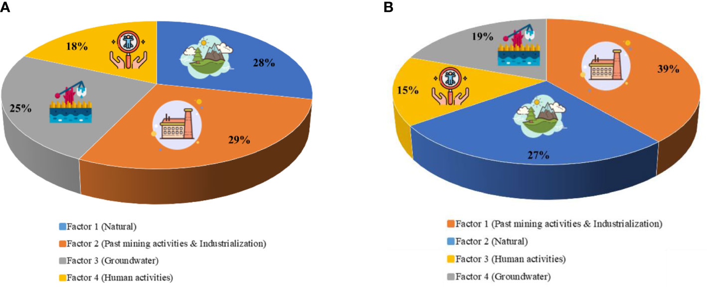
Figure 11 Source factorization of (A) recreational soil and (B) agricultural soil.

5. Conclusions

Through the use of numerous auxiliary data, this study created a unique integrated spatial technique for quantifying source apportionment and defining metal contamination in surface soils in Cerrito Blanco, Matehuala, San Luis Potosi, Mexico. The results of the metal concentrations in soils revealed that the mean concentrations of the selected eight metals in the soil were much higher than their specific permissible limits with the exception of Na. The mean concentration levels of heavy metals like As, Sr, Mn, and Fe were higher than their respective permissible limits by around 5.43, 2.57, 1.62, and 12.36 in recreational soil, and 3.50, 1.76, 3.29, and 23.11 times in agricultural soil. The results indicate that natural soil formation, contaminated groundwater use, and mining activities increased heavy metals in the topsoil. The I_geo was higher than zero for all selected metals, while the I_geo values of As and Fe were greater than one, which indicates that As and Fe were the main heavy metal elements that caused contamination in the recreational soil. Similarly, As, Mn and Fe were the key heavy metal elements that caused contamination in the agricultural soil. The mean value of the modified degree of contamination (mC_d) was 11.83, which indicates a very high degree of contamination in recreational soil and, mC_d for the agricultural soil was 19.38, which indicates an extreme degree of contamination. Moreover, the PI_N values of these two soils are 29.97 and 43.22, which confirms that the area is highly contaminated. According to the PMF results, the four potential source contributions of recreational and agricultural soil for metal concentrations in this study area are natural sources, past mining and industrial activities, irrigational groundwater, and human activities. The results of the source-specific risk assessment didn’t reflect the source apportionment factors for the concentration of metals; the order of the contribution of the risk factors in recreational soil was, factor 1 (28%, natural sources), factor 2 (29%, mining activities and industrialization), factor 3 (25%, groundwater sources), and factor 4 (18%, human activities). Similarly, in the agricultural soil, the corresponding contributions are factor 1 (39%, mining activities and industrialization), factor 2 (27%, natural sources), factor 3 (15%, human activities), and factor 4 (19%, groundwater sources). As explained, a 95.8% loading on factor 3 for contamination in recreational soil and 70.5% loading on factor 4 in agricultural soil due to irrigational groundwater sources, contributed primarily to the overall contamination risk. The contamination risk for As, Ca, Mg, K, Sr, Mn, and Fe indicated identical spatial distributions with high risk, except for Na. But it can be noted that some of these metals such as Ca, Mg, and K are not providing a significant risk for soil contamination despite being present in high amounts in soil, due to the beneficial role of these metals for soil health. The results of this study indicated that past mining activities and metallurgical pollution contributed most significantly to the contamination risk. In conclusion, further restrictions on the discharge of wastewater from mining industries, along with conventional emission controls, could be adopted to reduce contamination risks in soils. The results of the PMF model, GIS spatial distribution mapping, and contamination risk indices have significant implications for decision-makers to reduce threats to human health and environmental risk from possible sources of pollution.

Data availability statement

The datasets presented in this article are not readily available because they are subjected to funders’ regulations. Requests to access the datasets should be directed to the corresponding author.

Author contributions

AS: Conceptualization, Methodology, Software, Validation, Formal analysis, Resources, Writing - Original Draft, Visualization. BG: Conceptualization, Formal analysis, Investigation, Resources, Writing - Review & Editing, Supervision, Project administration, Funding acquisition. SP: Methodology, Data Curation, Writing - Review & Editing, Supervision. NM-V: Formal analysis, Investigation, Resources, Data Curation, Writing - Review & Editing. All authors contributed to the article and approved the submitted version.

Funding

The project has received funding from the Engineering and Physical Sciences Research Council (EPSRC-IAA), UKRI through the Project 748502: Spreading The Chemical Free Arsenic Removal Technology To Various Communities In India, Bangladesh And Mexico.

Acknowledgments

Thanks to the Institute of Infrastructure and Environment, EGIS, Heriot-Watt University, Edinburgh. The authors are thankful to The School of Energy, Geoscience, Infrastructure and Society (EGIS), Heriot-Watt University, Edinburgh for providing a student bursary to the first author for doctoral research through the James Watt Scholarship. The author would also thanks to IPICyT, San Luis Potosi, Mexico for providing feedback and support. We used Arsenic toxic metal data and GIS shapefile data while working on this study, and the data has been published previously in the International Journal of Environmental Research and Public Health, MDPI in 2018 and Journal of South American Earth Sciences, Elsevier in 2022 for a different type of study on toxic metal contamination. References to these studies are cited in the inner text.

Conflict of interest

The authors declare that the research was conducted in the absence of any commercial or financial relationships that could be construed as a potential conflict of interest.

Publisher’s note

All claims expressed in this article are solely those of the authors and do not necessarily represent those of their affiliated organizations, or those of the publisher, the editors and the reviewers. Any product that may be evaluated in this article, or claim that may be made by its manufacturer, is not guaranteed or endorsed by the publisher.

Supplementary material

The Supplementary Material for this article can be found online at: https://www.frontiersin.org/articles/10.3389/fsoil.2022.1041377/full#supplementary-material

References

1. Fei X, Christakos G, Xiao R, Ren Z, Liu Y, Lv X. Improved heavy metal mapping and pollution source apportionment in shanghai city soils using auxiliary information. Sci Total Environ. (2019) 661:168–77. doi: 10.1016/j.scitotenv.2019.01.149

PubMed Abstract | CrossRef Full Text | Google Scholar

2. He J, Yang Y, Christakos G, Liu Y, Yang X. Assessment of soil heavy metal pollution using stochastic site indicators. Geoderma (2019) 337:359–67. doi: 10.1016/j.geoderma.2018.09.038

CrossRef Full Text | Google Scholar

3. Wang S, Cai LM, Wen HH, Luo J, Wang QS, Liu X. Spatial distribution and source apportionment of heavy metals in soil from a typical county-level city of guangdong province, China. Sci Total Environ. (2019) 655:92–101. doi: 10.1016/j.scitotenv.2018.11.244

PubMed Abstract | CrossRef Full Text | Google Scholar

4. Fei X, Lou Z, Xiao R, Ren Z, Lv X. Contamination assessment and source apportionment of heavy metals in agricultural soil through the synthesis of PMF and GeogDetector models. Sci Total Environ. (2020) 747:141293. doi: 10.1016/j.scitotenv.2020.141293

PubMed Abstract | CrossRef Full Text | Google Scholar

5. Hu B, Jia X, Hu J, Xu D, Xia F, Li Y. Assessment of heavy metal pollution and health risks in the soil-plant-human system in the Yangtze river delta, China. Int J Environ Res Public Health (2017) 14(9):1042. doi: 10.3390/ijerph14091042

PubMed Abstract | CrossRef Full Text | Google Scholar

6. Karimi A, Haghnia GH, Ayoubi S, Safari T. Impacts of geology and land use on magnetic susceptibility and selected heavy metals in surface soils of mashhad plain, northeastern Iran. J Appl Geophys. (2017) 138:127–34. doi: 10.1016/j.jappgeo.2017.01.022

CrossRef Full Text | Google Scholar

7. Huang J, Guo S, Zeng GM, Li F, Gu Y, Shi Y, et al. A new exploration of health risk assessment quantification from sources of soil heavy metals under different land use. Environ pollut. (2018) 243:49–58. doi: 10.1016/j.envpol.2018.08.038

PubMed Abstract | CrossRef Full Text | Google Scholar

8. Yang Q, Li Z, Lu X, Duan Q, Huang L, Bi J. A review of soil heavy metal pollution from industrial and agricultural regions in China: Pollution and risk assessment. Sci total environ. (2018) 642:690–700. doi: 10.1016/j.scitotenv.2018.06.068

PubMed Abstract | CrossRef Full Text | Google Scholar

9. Azizi K, Ayoubi S, Nabiollahi K, Garosi Y, Gislum R. Predicting heavy metal contents by applying machine learning approaches and environmental covariates in west of Iran. J Geochem. Explor. (2022) 233:106921. doi: 10.1016/j.gexplo.2021.106921

CrossRef Full Text | Google Scholar

10. Chiprés JA, Castro-Larragoitia J, Monroy MG. Exploratory and spatial data analysis (EDA–SDA) for determining regional background levels and anomalies of potentially toxic elements in soils from catorce–matehuala, Mexico. Appl Geochem. (2009) 24(8):1579–89. doi: 10.1016/j.apgeochem.2009.04.022

CrossRef Full Text | Google Scholar

11. Mendoza Chávez YJ. Especies de zooplancton presentes en agua contaminada con arsénico en matehuala, San Luis potosí, méxico (2016). Available at: http://hdl.handle.net/11627/3009.

Google Scholar

12. Armienta MA, Segovia N. Arsenic and fluoride in the groundwater of Mexico. Environ Geochem. Health (2008) 30(4):345–53. doi: 10.1007/s10653-008-9167-8

PubMed Abstract | CrossRef Full Text | Google Scholar

13. Limón-Pacheco JH, Jiménez-Córdova MI, Cárdenas-González M, Retana IMS, Gonsebatt ME, Del Razo LM. Potential co-exposure to arsenic and fluoride and biomonitoring equivalents for Mexican children. Ann Global Health (2018) 84(2):257. doi: 10.29024/aogh.913

CrossRef Full Text | Google Scholar

14. Bundschuh J, Armienta MA, Morales-Simfors N, Alam MA, López DL, Delgado Quezada V, et al. Arsenic in Latin America: New findings on source, mobilization and mobility in human environments in 20 countries based on decadal research 2010-2020. Crit Rev Environ Sci technol. (2021) 51(16):1727–865. doi: 10.1080/10643389.2020.1770527

CrossRef Full Text | Google Scholar

15. Castro de Esparza MC. The presence of arsenic in drinking water in Latin America and its effect on public health. In: Natural arsenic in groundwater of Latin America. (London, United Kingdom, Taylor & Francis Ltd: CRC Press) (2009). p., vol. 1:17–29.

Google Scholar

16. Carrillo-Chávez A, Drever JI, Martínez M. Arsenic content and groundwater geochemistry of the San Antonio-El triunfo, carrizal and Los planes aquifers in southernmost Baja California, Mexico. Environ Geol. (2000) 39(11):1295–303. doi: 10.1007/s002540000153

CrossRef Full Text | Google Scholar

17. Talavera Mendoza O, Armienta Hernández MA, Abundis JG, Mundo NF. Geochemistry of leachates from the El fraile sulfide tailings piles in taxco, Guerrero, southern Mexico. Environ geochem. Health (2006) 28(3):243–55. doi: 10.1007/s10653-005-9037-6

PubMed Abstract | CrossRef Full Text | Google Scholar

18. Martínez-Villegas N, Briones-Gallardo R, Ramos-Leal JA, Avalos-Borja M, Castañón-Sandoval AD, Razo-Flores E, et al. Arsenic mobility controlled by solid calcium arsenates: A case study in Mexico showcasing a potentially widespread environmental problem. Environ Pollut. (2013) 176:114–22. doi: 10.1016/j.envpol.2012.12.025

PubMed Abstract | CrossRef Full Text | Google Scholar

19. Saha A, Gupta BS, Patidar S, Martínez-Villegas N. Spatial distribution based on optimal interpolation techniques and assessment of contamination risk for toxic metals in the surface soil. J South Am Earth Sci (2022) 115:103763. doi: 10.1016/j.jsames.2022.103763

CrossRef Full Text | Google Scholar

20. Ruíz-Huerta EA, de la Garza Varela A, Gómez-Bernal JM, Castillo F, Avalos-Borja M, SenGupta B, et al. Arsenic contamination in irrigation water, agricultural soil and maize crop from an abandoned smelter site in matehuala, Mexico. J hazard. materi. (2017) 339:330–9. doi: 10.1016/j.jhazmat.2017.06.041

CrossRef Full Text | Google Scholar

21. Aguilera A, Cortés JL, Delgado C, Aguilar Y, Aguilar D, Cejudo R, et al. Heavy metal contamination (Cu, Pb, zn, fe, and Mn) in urban dust and its possible ecological and human health risk in Mexican cities. Front Environ Sci. (2022) 195:854460. doi: 10.3389/fenvs.2022.854460

CrossRef Full Text | Google Scholar

22. Saha A, Gupta BS, Patidar S, Martínez-Villegas N. Evaluation of potential ecological risk index of toxic metals contamination in the soils. IOCAG Chem Proc (2022) 10(1):59. doi: 10.3390/IOCAG2022-12214

CrossRef Full Text | Google Scholar

23. Yang S, Zhou D, Yu H, Wei R, Pan B. Distribution and speciation of metals (Cu, zn, cd, and Pb) in agricultural and non-agricultural soils near a stream upriver from the pearl river, China. Environ Pollut. (2013) 177:64–70. doi: 10.1016/j.envpol.2013.01.044

PubMed Abstract | CrossRef Full Text | Google Scholar

24. Shen W, Hu Y, Zhang J, Zhao F, Bian P, Liu Y. Spatial distribution and human health risk assessment of soil heavy metals based on sequential Gaussian simulation and positive matrix factorization model: A case study in irrigation area of the yellow river. Ecotoxicol. Environ Safety. (2021) 225:112752. doi: 10.1016/j.ecoenv.2021.112752

CrossRef Full Text | Google Scholar

25. Miao F, Zhang Y, Li Y, Fang Q, Zhou Y. Implementation of an integrated health risk assessment coupled with spatial interpolation and source contribution: A case study of soil heavy metals from an abandoned industrial area in suzhou, China. In: Stochastic environmental research and risk assessment (Springer-Verlag GmbH Germany: Springer Nature) (2022). 36:2633–47. doi: 10.1007/s00477-021-02146-2

CrossRef Full Text | Google Scholar

26. Xu Y, Wang X, Cui G, Li K, Liu Y, Li B, et al. Source apportionment and ecological and health risk mapping of soil heavy metals based on PMF, SOM, and GIS methods in hulan river watershed, northeastern China. Environ Monit Assess. (2022) 194(3):1–17. doi: 10.1007/s10661-022-09826-8

CrossRef Full Text | Google Scholar

27. Taghipour M, Ayoubi S, Khademi H. Contribution of lithologic and anthropogenic factors to surface soil heavy metals in western Iran using multivariate geostatistical analyses. Soil Sediment Contam.: Int J (2011) 20(8):921–37. doi: 10.1080/15320383.2011.620045

CrossRef Full Text | Google Scholar

28. Zhang P, Qin C, Hong X, Kang G, Qin M, Yang D, et al. Risk assessment and source analysis of soil heavy metal pollution from lower reaches of yellow river irrigation in China. Sci Total Environ. (2018) 633:1136–47. doi: 10.1016/j.scitotenv.2018.03.228

PubMed Abstract | CrossRef Full Text | Google Scholar

29. Zhang X, Wei S, Sun Q, Wadood SA, Guo B. Source identification and spatial distribution of arsenic and heavy metals in agricultural soil around hunan industrial estate by positive matrix factorization model, principle components analysis and geo statistical analysis. Ecotoxicol. Environ safety. (2018) 159:354–62. doi: 10.1016/j.ecoenv.2018.04.072

CrossRef Full Text | Google Scholar

30. Su C, Meng J, Zhou Y, Bi R, Chen Z, Diao J, et al. Heavy metals in soils from intense industrial areas in south China: Spatial distribution, source apportionment, and risk assessment. Front Environ Sci (2022) 10:820536. doi: 10.3389/fenvs.2022.820536

CrossRef Full Text | Google Scholar

31. Su H, Hu Y, Wang L, Yu H, Li B, Liu J. Source apportionment and geographic distribution of heavy metals and as in soils and vegetables using kriging interpolation and positive matrix factorization analysis. Int J Environ Res Public Health (2022) 19(1):485. doi: 10.3390/ijerph19010485

PubMed Abstract | CrossRef Full Text | Google Scholar

32. González-Macías C, Sánchez-Reyna G, Salazar-Coria L, Schifter I. Application of the positive matrix factorization approach to identify heavy metal sources in sediments. a case study on the Mexican pacific coast. Environ Monit assess. (2014) 186(1):307–24. doi: 10.1007/s10661-013-3375-0

PubMed Abstract | CrossRef Full Text | Google Scholar

33. Xu Y, Shi H, Fei Y, Wang C, Mo L, Shu M. Identification of soil heavy metal sources in a large-scale area affected by industry. Sustainability (2021) 13(2):511. doi: 10.3390/su13020511

CrossRef Full Text | Google Scholar

34. Yu D, Wang J, Wang Y, Du X, Li G, Li B. Identifying the source of heavy metal pollution and apportionment in agricultural soils impacted by different smelters in China by the positive matrix factorization model and the Pb isotope ratio method. Sustainability (2021) 13(12):6526. doi: 10.3390/su13126526

CrossRef Full Text | Google Scholar

35. Li F, Xiang M, Yu S, Xia F, Li Y, Shi Z. Source identification and apportionment of potential toxic elements in soils in an Eastern industrial city, China. Int J Environ Res Public Health (2022) 19(10):6132. doi: 10.3390/ijerph19106132

PubMed Abstract | CrossRef Full Text | Google Scholar

36. Wang S, Zhang Y, Cheng J, Li Y, Li F, Li Y, et al. Pollution assessment and source apportionment of soil heavy metals in a coastal industrial city, zhejiang, southeastern China. Int J Environ Res Public Health (2022) 19(6):3335. doi: 10.3390/ijerph19063335

PubMed Abstract | CrossRef Full Text | Google Scholar

37. Wang Z, Shen Q, Hua P, Jiang S, Li R, Li Y, et al. Characterizing the anthropogenic-induced trace elements in an urban aquatic environment: A source apportionment and risk assessment with uncertainty consideration. J Environ Manage. (2020) 275:111288. doi: 10.1016/j.jenvman.2020.111288

PubMed Abstract | CrossRef Full Text | Google Scholar

38. Li Q, Zhang J, Ge W, Sun P, Han Y, Qiu H, et al. Geochemical baseline establishment and source-oriented ecological risk assessment of heavy metals in lime concretion black soil from a typical agricultural area. Int J Environ Res Public Health (2021) 18(13):6859. doi: 10.3390/ijerph18136859

PubMed Abstract | CrossRef Full Text | Google Scholar

39. Proshad R, Uddin M, Idris AM, Al MA. Receptor model-oriented sources and risks evaluation of metals in sediments of an industrial affected riverine system in Bangladesh. Sci Total Environ. (2022), 838:156029. doi: 10.1016/j.scitotenv.2022.156029

PubMed Abstract | CrossRef Full Text | Google Scholar

40. Shi W, Li T, Feng Y, Su H, Yang Q. Source apportionment and risk assessment for available occurrence forms of heavy metals in dongdahe wetland sediments, southwest of China. Sci Total Environ. (2022) 815:152837. doi: 10.1016/j.scitotenv.2021.152837

PubMed Abstract | CrossRef Full Text | Google Scholar

41. Abrahim GMS, Parker RJ. Assessment of heavy metal enrichment factors and the degree of contamination in marine sediments from tamaki estuary, Auckland, new Zealand. Environ Monit assess. (2008) 136(1):227–38. doi: 10.1007/s10661-007-9678-2

PubMed Abstract | CrossRef Full Text | Google Scholar

42. Hu Y, Liu X, Bai J, Shih K, Zeng EY, Cheng H. Assessing heavy metal pollution in the surface soils of a region that had undergone three decades of intense industrialization and urbanization. Environ Sci pollut Res (2013) 20(9):6150–9. doi: 10.1007/s11356-013-1668-z

CrossRef Full Text | Google Scholar

43. Qi Z, Gao X, Qi Y, Li J. Spatial distribution of heavy metal contamination in mollisol dairy farm. Environ Pollut. (2020) 263:114621. doi: 10.1016/j.envpol.2020.114621

CrossRef Full Text | Google Scholar

44. Maurya P, Kumari R. Toxic metals distribution, seasonal variations and environmental risk assessment in surficial sediment and mangrove plants (A. marina), gulf of kachchh (India). J Hazard. Mater. (2021) 413:125345. doi: 10.1016/j.jhazmat.2021.125345

PubMed Abstract | CrossRef Full Text | Google Scholar

45. Ayoubi S, Amiri S, Tajik S. Lithogenic and anthropogenic impacts on soil surface magnetic susceptibility in an arid region of central Iran. Arch Agron Soil Sci. (2014) 60(10):1467–83. doi: 10.1080/03650340.2014.893574

CrossRef Full Text | Google Scholar

46. Agyeman PC, John K, Kebonye NM, Borůvka L, Vašát R, Drábek O. A geostatistical approach to estimating source apportionment in urban and peri-urban soils using the Czech republic as an example. Sci Rep (2021) 11(1):1–15. doi: 10.1038/s41598-021-02968-8

PubMed Abstract | CrossRef Full Text | Google Scholar

47. Luo P, Xu C, Kang S, Huo A, Lyu J, Zhou M, et al. Heavy metals in water and surface sediments of the fenghe river basin, China: Assessment and source analysis. Water Sci Technol. (2021) 84(10-11):3072–90. doi: 10.2166/wst.2021.335

PubMed Abstract | CrossRef Full Text | Google Scholar

48. Ma J, Chen Y, Weng L, Peng H, Liao Z, Li Y. Source identification of heavy metals in surface paddy soils using accumulated elemental ratios coupled with MLR. Int J Environ Res Public Health (2021) 18(5):2295. doi: 10.3390/ijerph18052295

PubMed Abstract | CrossRef Full Text | Google Scholar

49. Zhao X, Li Z, Wang D, Tao Y, Qiao F, Lei L, et al. Characteristics, source apportionment and health risk assessment of heavy metals exposure via household dust from six cities in China. Sci Total Environ. (2021) 762:143126. doi: 10.1016/j.scitotenv.2020.143126

PubMed Abstract | CrossRef Full Text | Google Scholar

50. Wu J, Li J, Teng Y, Chen H, Wang Y. A partition computing-based positive matrix factorization (PC-PMF) approach for the source apportionment of agricultural soil heavy metal contents and associated health risks. J Hazard. Mater. (2020) 388:121766. doi: 10.1016/j.jhazmat.2019.121766

PubMed Abstract | CrossRef Full Text | Google Scholar

51. Kim E, Hopke PK, Larson TV, Covert DS. Analysis of ambient particle size distributions using unmix and positive matrix factorization. Environ Sci technol. (2004) 38(1):202–9. doi: 10.1021/es030310s

PubMed Abstract | CrossRef Full Text | Google Scholar

52. Schaefer K, Einax JW. Source apportionment and geostatistics: An outstanding combination for describing metals distribution in soil. CLEAN–Soil Air Water. (2016) 44(7):877–84. doi: 10.1002/clen.201400459

CrossRef Full Text | Google Scholar

53. Chen H, Teng Y, Lu S, Wang Y, Wu J, Wang J. Source apportionment and health risk assessment of trace metals in surface soils of Beijing metropolitan, China. Chemosphere (2016) 144:1002–11. doi: 10.1016/j.chemosphere.2015.09.081

PubMed Abstract | CrossRef Full Text | Google Scholar

54. Ma W, Tai L, Qiao Z, Zhong L, Wang Z, Fu K, et al. Contamination source apportionment and health risk assessment of heavy metals in soil around municipal solid waste incinerator: A case study in north China. Sci Total Environ. (2018) 631:348–57. doi: 10.1016/j.scitotenv.2018.03.011

PubMed Abstract | CrossRef Full Text | Google Scholar

55. Adgate JL, Willis RD, Buckley TJ, Chow JC, Watson JG, Rhoads GG, et al. Chemical mass balance source apportionment of lead in house dust. Environ Sci technol. (1998) 32(1):108–14. doi: 10.1021/es970052x

CrossRef Full Text | Google Scholar

56. Lv J, Liu Y. An integrated approach to identify quantitative sources and hazardous areas of heavy metals in soils. Sci Total Environ. (2019) 646:19–28. doi: 10.1016/j.scitotenv.2018.07.257

PubMed Abstract | CrossRef Full Text | Google Scholar

57. Jorquera H, Barraza F. Source apportionment of PM10 and PM2. 5 in a desert region in northern Chile. Sci Total Environ. (2013) 444:327–35. doi: 10.1016/j.scitotenv.2012.12.007

PubMed Abstract | CrossRef Full Text | Google Scholar

58. Ahmed F, Fakhruddin ANM, Imam MD, Khan N, Khan TA, Rahman M, et al. Spatial distribution and source identification of heavy metal pollution in roadside surface soil: a study of Dhaka aricha highway, Bangladesh. Ecol processes. (2016) 5(1):1–16. doi: 10.1186/s13717-016-0045-5

CrossRef Full Text | Google Scholar

59. Feng J, Song N, Yu Y, Li Y. Differential analysis of FA-NNC, PCA-MLR, and PMF methods applied in source apportionment of PAHs in street ust. Environ Monit assess. (2020) 192(11):1–11. doi: 10.1007/s10661-020-08679-3

CrossRef Full Text | Google Scholar

60. Men C, Liu R, Wang Q, Guo L, Miao Y, Shen Z. Uncertainty analysis in source apportionment of heavy metals in road dust based on positive matrix factorization model and geographic information system. Sci Total Environ. (2019) 652:27–39. doi: 10.1016/j.scitotenv.2018.10.212

PubMed Abstract | CrossRef Full Text | Google Scholar

61. Chai L, Wang Y, Wang X, Ma L, Cheng Z, Su L, et al. Quantitative source apportionment of heavy metals in cultivated soil and associated model uncertainty. Ecotoxicol. Environ Safety. (2021) 215:112150. doi: 10.1016/j.ecoenv.2021.112150

CrossRef Full Text | Google Scholar

62. Liu R, Men C, Yu W, Xu F, Wang Q, Shen Z. Uncertainty in positive matrix factorization solutions for PAHs in surface sediments of the Yangtze river estuary in different seasons. Chemosphere (2018) 191:922–36. doi: 10.1016/j.chemosphere.2017.10.070

PubMed Abstract | CrossRef Full Text | Google Scholar

63. Perrone MG, Vratolis S, Georgieva E, Török S, Šega K, Veleva B, et al. Sources and geographic origin of particulate matter in urban areas of the Danube macro-region: The cases of Zagreb (Croatia), Budapest (Hungary) and Sofia (Bulgaria). Sci Total Environ. (2018) 619:1515–29. doi: 10.1016/j.scitotenv.2017.11.092

PubMed Abstract | CrossRef Full Text | Google Scholar

64. Dong B, Zhang R, Gan Y, Cai L, Freidenreich A, Wang K, et al. Multiple methods for the identification of heavy metal sources in cropland soils from a resource-based region. Sci Total Environ. (2019) 651:3127–38. doi: 10.1016/j.scitotenv.2018.10.130

PubMed Abstract | CrossRef Full Text | Google Scholar

65. Castro-Larragoitia J, Kramar U, Puchelt H. 200 years of mining activities at la Paz/San Luis Potosí/Mexico–consequences for environment and geochemical exploration. J Geochem. Explor. (1997) 58(1):81–91. doi: 10.1016/S0375-6742(96)00054-4

CrossRef Full Text | Google Scholar

66. Razo I, Carrizales L, Castro J, Díaz-Barriga F, Monroy M. Arsenic and heavy metal pollution of soil, water and sediments in a semi-arid climate mining area in Mexico. Water Air Soil Pollut. (2004) 152(1):129–52. doi: 10.1023/B:WATE.0000015350.14520.c1

CrossRef Full Text | Google Scholar

67. Martínez-Villegas N, Hernández A, Meza-Figueroa D, Sen Gupta B. Distribution of arsenic and risk assessment of activities on soccer pitches irrigated with arsenic-contaminated water. Int J Environ Res Public Health (2018) 15(6):1060. doi: 10.3390/ijerph15061060

PubMed Abstract | CrossRef Full Text | Google Scholar

68. Yáñez L, Garcı́a-Nieto E, Rojas E, Carrizales L, Mejı́a J, Calderón J, et al. DNA Damage in blood cells from children exposed to arsenic and lead in a mining area. Environ Res (2003) 93(3):231–40. doi: 10.1016/j.envres.2003.07.005

PubMed Abstract | CrossRef Full Text | Google Scholar

69. Mendoza-Chávez YJ, Uc-Castillo JL, Cervantes-Martínez A, Gutiérrez-Aguirre MA, Castillo-Michel H, Loredo-Portales R, et al. Paracyclops chiltoni inhabiting water highly contaminated with arsenic: Water chemistry, population structure, and arsenic distribution within the organism. Environ Pollut. (2021) 284:117155. doi: 10.1016/j.envpol.2021.117155

PubMed Abstract | CrossRef Full Text | Google Scholar

70. INEGI. Prontuario de información geográfica municipal de los estados unidos mexicanos Vol. 2009. . Aguascalientes, México: Instituto Nacional de Estadística Geografía e Informática (2009).

Google Scholar

71. Secretaria de Economía. NMX-AA-132-SCFI-2001–muestreo de suelos para la identificación y la cuantificación de metales y metaloides, y manejo de la muestra. México City, México: Secretaria de Economía (2006). p. 32.

Google Scholar

72. USEPA. Method 200.7: Revision 4.4, determination of metals and trace elements in water and wastes by inductively coupled plasma-atomic emission spectrometry. Cincinnati, OH, USA: United States Environmental Protection Agency (1994).

Google Scholar

73. McCoy J, Johnston K. Using ArcGIS spatial analyst ESRI Vol. 2002. . California, USA: Redlands (2001).

Google Scholar

74. Arumugam T, Kunhikannan S, Radhakrishnan P. Assessment of fluoride hazard in groundwater of palghat district, kerala: A GIS approach. Int J Environ Pollut. (2019) 66(1-3):187–211. doi: 10.1504/IJEP.2019.104533

CrossRef Full Text | Google Scholar

75. Li F, Huang J, Zeng G, Yuan X, Li X, Liang J, et al. Spatial risk assessment and sources identification of heavy metals in surface sediments from the dongting lake, middle China. J Geochem. Explor. (2013) 132:75–83. doi: 10.1016/j.gexplo.2013.05.007

CrossRef Full Text | Google Scholar

76. Dai L, Wang L, Li L, Liang T, Zhang Y, Ma C, et al. Multivariate geostatistical analysis and source identification of heavy metals in the sediment of poyang lake in China. Sci total environ. (2018) 621:1433–44. doi: 10.1016/j.scitotenv.2017.10.085

PubMed Abstract | CrossRef Full Text | Google Scholar

77. Keshavarzi A, Sarmadian F. Mapping of spatial distribution of soil salinity and alkalinity in a semi-arid region. Ann Warsaw Univ Life Sciences-SGGW. Land Reclam. (2012) 44(1):3–14. doi: 10.2478/v10060-011-0057-x

CrossRef Full Text | Google Scholar

78. Bhunia GS, Shit PK, Maiti R. Comparison of GIS-based interpolation methods for spatial distribution of soil organic carbon (SOC). J Saudi Soc Agric Sci (2018) 17(2):114–26. doi: 10.1016/j.jssas.2016.02.001

CrossRef Full Text | Google Scholar

79. Tong S, Li H, Wang L, Tudi M, Yang L. Concentration, spatial distribution, contamination degree and human health risk assessment of heavy metals in urban soils across China between 2003 and 2019–a systematic review. Int J Environ Res Public Health (2020) 17(9):3099. doi: 10.3390/ijerph17093099

PubMed Abstract | CrossRef Full Text | Google Scholar

80. Muller G. Index of geoaccumulation in sediments of the Rhine river. Geojournal (1969) 2:108–18.

Google Scholar

81. Rutkowski P, Diatta J, Konatowska M, Andrzejewska A, Tyburski Ł., Przybylski P. Geochemical referencing of natural forest contamination in Poland. Forests (2020) 11(2):157. doi: 10.3390/f11020157

CrossRef Full Text | Google Scholar

82. Hakanson L. An ecological risk index for aquatic pollution control. a sedimentological approach. Water Res (1980) 14(8):975–1001. doi: 10.1016/0043-1354(80)90143-8

CrossRef Full Text | Google Scholar

83. Wang X, Deng C, Yin J, Tang X. (2018). Toxic heavy metal contamination assessment and speciation in sugarcane soil, in: IOP Conference Series: Earth and Environmental Science, , Vol. 108. p. 042059. IOP Publishing. doi: 10.1088/1755-1315/108/4/042059

CrossRef Full Text | Google Scholar

84. Abrahim GMS. Holocene Sediments of tamaki estuary: Characterisation and impact of recent human activity on an urban estuary in Auckland, new Zealand Vol. 361. . Auckland, New Zealand: University of Auckland (2005).

Google Scholar

85. Cheng JL, Zhou SHI, Zhu YW. Assessment and mapping of environmental quality in agricultural soils of zhejiang province, China. J Environ Sci (2007) 19(1):50–4. doi: 10.1016/S1001-0742(07)60008-4

CrossRef Full Text | Google Scholar

86. Joy A, Anoop PP, Rajesh R, Mathew A, Gopinath A. Spatial distribution and contamination assessment of trace metals in the coral reef sediments of kavaratti island in Lakshadweep archipelago, Indian ocean. Soil Sediment Contam.: Int J (2020) 29(2):209–31. doi: 10.1080/15320383.2019.1699899

CrossRef Full Text | Google Scholar

87. Ahamad A, Raju NJ, Madhav S, Gossel W, Ram P, Wycisk P. Potentially toxic elements in soil and road dust around sonbhadra industrial region, uttar pradesh, India: Source apportionment and health risk assessment. Environ Res (2021) 202:111685. doi: 10.1016/j.envres.2021.111685

PubMed Abstract | CrossRef Full Text | Google Scholar

88. Hoang HG, Lin C, Tran HT, Chiang CF, Bui XT, Cheruiyot NK, et al. Heavy metal contamination trends in surface water and sediments of a river in a highly-industrialized region. Environ Technol Innov. (2020) 20:101043. doi: 10.1016/j.eti.2020.101043

CrossRef Full Text | Google Scholar

89. Custodio M, Espinoza C, Orellana E, Chanamé F, Fow A, Peñaloza R. Assessment of toxic metal contamination, distribution and risk in the sediments from lagoons used for fish farming in the central region of Peru. Toxicol Rep (2022) 9:1603–13. doi: 10.1016/j.toxrep.2022.07.016

CrossRef Full Text | Google Scholar

90. Cai L, Huang L, Zhou Y, Xu Z, Peng X, Yao LA, et al. Heavy metal concentrations of agricultural soils and vegetables from dongguan, guangdong. J Geogr. Sci (2010) 20(1):121–34. doi: 10.1007/s11442-010-0121-1

CrossRef Full Text | Google Scholar

91. Yan N, Liu W, Xie H, Gao L, Han Y, Wang M, et al. Distribution and assessment of heavy metals in the surface sediment of yellow river, China. J Environ Sci (2016) 39:45–51. doi: 10.1016/j.jes.2015.10.017

CrossRef Full Text | Google Scholar

92. United States Environmental Protection Agency. EPA Positive matrix factorization (PMF) 5.0 fundamentals and user guide. (Washington, DC:United States Environmental Protection Agency) (2014).

Google Scholar

93. Paatero P, Tapper U. Positive matrix factorization: A non-negative factor model with optimal utilization of error estimates of data values. Environmetrics (1994) 5(2):111–26. doi: 10.1002/env.3170050203

CrossRef Full Text | Google Scholar

94. Kuerban M, Maihemuti B, Waili Y, Tuerhong T. Ecological risk assessment and source identification of heavy metal pollution in vegetable bases of urumqi, China, using the positive matrix factorization (PMF) method. PloS One (2020) 15(4):e0230191. doi: 10.1371/journal.pone.0230191

PubMed Abstract | CrossRef Full Text | Google Scholar

95. USEPA. Definition and procedure for the determination of the method detection limit, revision 2 (2016). Available at: https://www.epa.gov/sites/default/files/2016-12/documents/mdl-procedure_rev2_12-13-2016.pdf.

Google Scholar

96. Paatero P, Eberly S, Brown SG, Norris GA. Methods for estimating uncertainty in factor analytic solutions. Atmos. Meas. Tech. (2014) 7(3):781–97. doi: 10.5194/amt-7-781-2014

CrossRef Full Text | Google Scholar

97. Secretaria de Medio Ambiente Y Recursos Naturales. (2004). Available at: http://www.profepa.gob.mx/innovaportal/file/1392/1/nom-147-semarnat_ssa1-2004.pdf.

Google Scholar

98. Imran M, Kanwal F, Liviu M, Amir M, Iqbal MA. Evaluation of physico-chemical characteristics of soil samples collected from harrapa-sahiwal (Pakistan). Asian J Chem (2010) 22(6):4823.

Google Scholar

99. Essel KK. Heavy metals geochemistry in selected districts of upper east region soils, Ghana. Environ Earth Sci (2017) 76(10):1–10. doi: 10.1007/s12665-017-6661-2

CrossRef Full Text | Google Scholar

100. Ashraf I, Ahmad F, Sharif A, Altaf AR, Teng H. Heavy metals assessment in water, soil, vegetables and their associated health risks via consumption of vegetables, district kasur, Pakistan. SN Appl Sci (2021) 3(5):1–16. doi: 10.1007/s42452-021-04547-y

CrossRef Full Text | Google Scholar

101. Iyama WA, Okpara K, Techato K. Assessment of heavy metals in agricultural soils and plant (Vernonia amygdalina delile) in port Harcourt metropolis, Nigeria. Agriculture (2021) 12(1):27. doi: 10.3390/agriculture12010027

CrossRef Full Text | Google Scholar

102. Liu H, Anwar S, Fang L, Chen L, Xu W, Xiao L, et al. Source apportionment of agricultural soil heavy metals based on PMF model and multivariate statistical analysis. Environ Forensics. (2022), 23:1–9. doi: 10.1080/15275922.2022.2047838

CrossRef Full Text | Google Scholar

103. Wilding LP. Spatial variability: Its documentation, accomodation and implication to soil surveys. In: Soil spatial variability, vol. 1984. (Las Vegas NV:Pudoc, Wageningen) (1985). p. 166–94. Available at: http://pascal-francis.inist.fr/vibad/index.php?action=getRecordDetail&idt=8485840.

Google Scholar

104. He K, Sun Z, Hu Y, Zeng X, Yu Z, Cheng H. Comparison of soil heavy metal pollution caused by e-waste recycling activities and traditional industrial operations. Environ Sci pollut Res (2017) 24(10):9387–98. doi: 10.1007/s11356-017-8548-x

CrossRef Full Text | Google Scholar

105. Guan Q, Wang F, Xu C, Pan N, Lin J, Zhao R, et al. Source apportionment of heavy metals in agricultural soil based on PMF: A case study in hexi corridor, northwest China. Chemosphere (2018) 193:189–97. doi: 10.1016/j.chemosphere.2017.10.151

PubMed Abstract | CrossRef Full Text | Google Scholar

106. Pinsino A, Matranga V, Roccheri MC. Manganese: A new emerging contaminant in the environment. In: Environmental contamination (Rijeka, Croatia: InTech) (2012). p. 17–36.

Google Scholar

107. Jamshidi-Zanjani A, Saeedi M. Metal pollution assessment and multivariate analysis in sediment of anzali international wetland. Environ Earth Sci (2013) 70(4):1791–808. doi: 10.1007/s12665-013-2267-5

CrossRef Full Text | Google Scholar