Assessing soil moisture variability in a vineyard via frequency domain electromagnetic induction data

1 Introduction

Over the last few decades, the high demand for water for agriculture and potable use has required an improvement in water management efficiency. Groundwater extraction through pumping is essential to provide irrigation water for crop growth but, in water-scarce coastal areas, its overexploitation increases the pressure on water resources. In fact, saltwater intrusion has negative consequences in terms of groundwater quality degradation and soil salinization, by reducing the freshwater available to coastal communities. On the other hand, the decreased water supply due to reduced rainfall and climate change effects caused by global warming are expected to have substantial impacts on global water resources in the next decades.

For all these reasons, accurate soil moisture information is essential to infer water requirements for hydrological modeling, as well as for appropriate water management. Detailed predictive models rely on accurate measurements that can be spatially distributed and updated over time. The point-scale sensors typically used for these purposes, such as Time Domain Reflectometry (TDR), Time Domain Transmissometry (TDT), and capacitive sensors, provide accurate but sparse information about soil properties, being unable to capture the soil heterogeneities due to their own point-source nature. On the other hand, It is unrealistic to install a large number of such sensors, both on the surface and at different depths, to capture the spatial distribution of the soil properties. In the last decade geophysical measurements have been increasingly used for spatio-temporal monitoring because they do not alter the soil properties, being non-invasive or minimally invasive. In addition, geophysical methods allow the collection of data over broad areas at different depths and in a relatively short time by providing high spatial coverage of the investigated soil with a resolution comparable with that obtained from sensors, in some cases. Finally, repeated time-lapse measurements allow data to be updated over time in order to capture changes in soil moisture that are otherwise undetectable with traditional devices. Among several geophysical methods, frequency domain electromagnetic induction (FDEM or EMI) is a promising tool for providing an accurate estimate of soil hydrological properties because of the high sensitivity of the electrical conductivity, i.e., the output geophysical parameter, to soil moisture and salinity. In fact, the main contribution to electrical conductivity is provided by the electrical conduction that occurs in soil by fluid conduction—i.e., electrolytic conduction by ionic transfer in pore water. Other factors that affect the electrical conductivity of the soil include porosity, soil texture, and soil temperature (1). Compared to sensors, coring, and other geophysical methods, FDEM data can provide essential subsurface information over large areas in conductive environments because they are on-the-go field measurements. An extensive literature refers to the use of FDEM measurements for mapping geological, hydrogeological, and environmental features. Weymer et al. (2) reviewed applications of the EMI technique for mapping barrier island framework geology, emphasizing the benefits for identifying buried geological structures and supporting conventional geological methods. Paepen et al. (3) provided a high-resolution 3D image of the saltwater and freshwater distribution in a coastal aquifer through a combination of EMI and electrical resistivity tomography (ERT) measurements. McLachlan et al. (4) highlighted the potential of EMI methods to characterize the hydrogeological structures of a riparian wetland in combination with electrical resistivity tomography (ERT) data. Deidda et al. (5) demonstrated the capability of the EMI tool to characterize anthropic facilities, such as capped landfills, in order to protect and/or remediate the main environmental compartments involved, such as water, soil, and subsoil. Two different approaches concerning FDEM data processing are currently used. Several case studies report the use of the apparent electrical conductivity, ECa or σ_a, as a proxy parameter for visualizing soil spatial variability, which, in turn, is converted to chemical and/or hydrological properties (6–27). Although widely used for a rapid visualization of the soil electrical properties, ECa values reflect different but overlapping soil volumes. ECa is a depth-weighted parameter and gives limited information about the variation of the conductivity with depth. In fact, ECa does not provide a rigorous correlation between the soil conductivity structure and measured responses, being affected by several factors such as coil distance and orientation, sensitivity, and data error. In the last few years, a numerical procedure based on inversion of the electromagnetic data has been refined. This approach provides a rigorous soil electromagnetic modeling (28–44) by improving the resolution of subsurface features and the assessment of the soil properties. Nevertheless, the smoothness-constrained regularization term (45) included during the iterative process for solving the nonlinearity of the inversion problem introduces some degrees of uncertainty in the resulting model, suggesting that these data should be treated as “soft” or even qualitative information (46). Beyond that, translating the geophysical outputs into hydrological ones is not a trivial issue. The well-established petrophysical relationships (47–49) or site-specific calibration functions commonly used in agrigeophysics are typically calibrated on small soil samples, leading to potential artifacts or unrealistic estimations when upscaled to ground-based measurements. According to these premises, the purpose of the present work is to provide a contribution to the scientific community for improving the quantitative integration of invasive and non-invasive soil measurements. In the proposed case study, an innovative and integrated assessment approach based on a freeware data-analysis tool licensed from USGS, MoisturEC, was tested on an experimental vineyard. Soil moisture data and electrical conductivity estimations inferred from the inversion of ECa measurements were used as input for the code with the aim of 1) providing accurate soil moisture estimations in a vineyard, 2) reducing the gap in terms of spatial variability between the dense geophysical data and sparse soil moisture measurements, and 3) incorporating the aforementioned data and model uncertainty in the hydrological estimation.

2 Material and methods

2.1 Study area

The experimental field is a vineyard that laps the Natural Reserve of Torre Guaceto, Apulia Region, Southern Italy (737212 E – 4508502 N WGS UTM84, altitude 10 m asl). The vineyard, located less than 1 km from the coastline, belongs to the Greco Farm, covering 4.5 hectares (Figure 1). The soil is a Colluvic Regosol consisting of silt and silty loam with an average depth of 50 cm. During the growth season, the vineyard is irrigated with groundwater extracted from the nearby pumping wells.

Figure 1

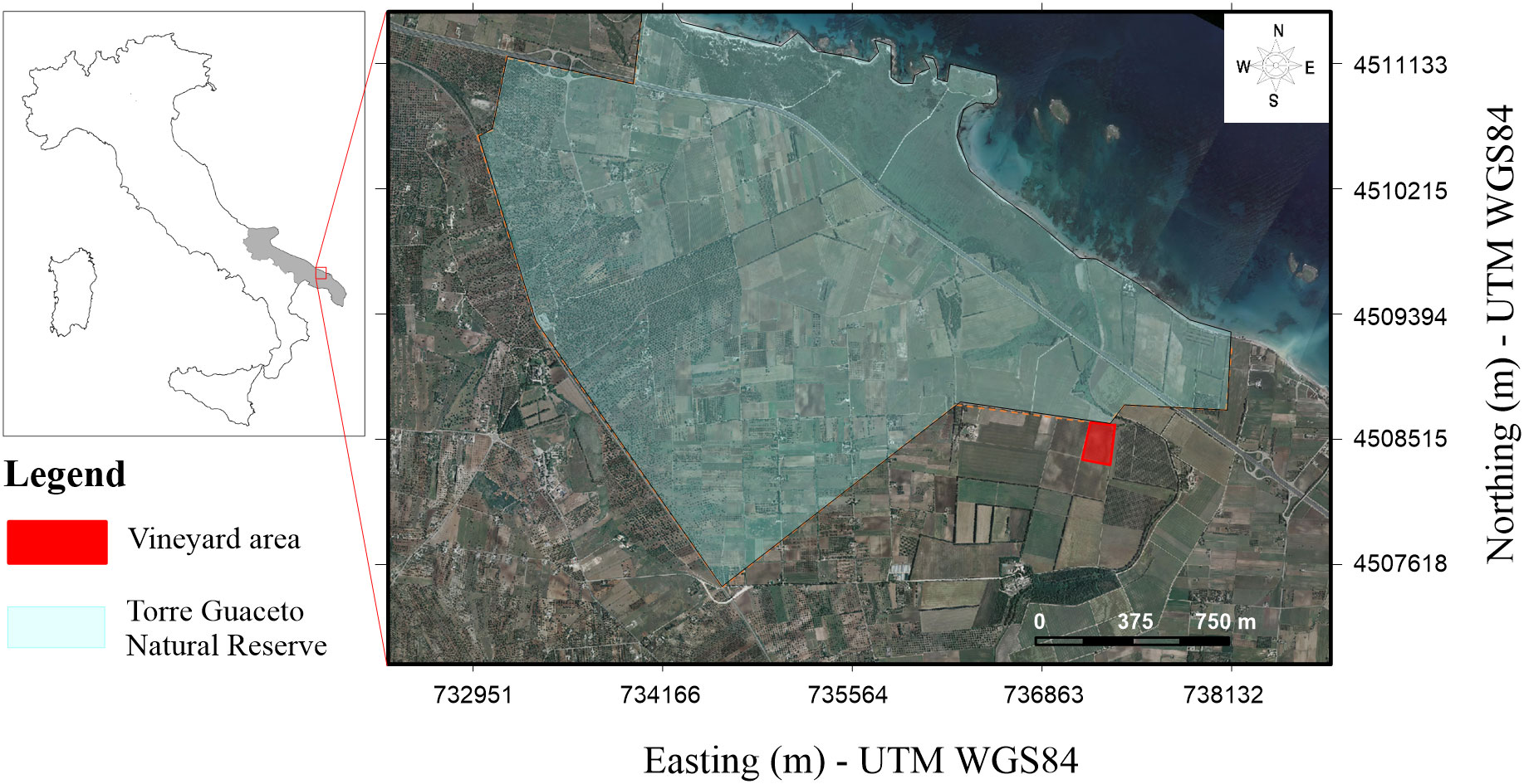
Figure 1 Location of the study area including the boundaries of the Natural Reserve of Torre Guaceto (dotted orange line and light green filling) and the experimental plot (red filling). The map coordinates are in WGS84/UTM33N (EPSG:32633).

2.2 Field data collection

In March 2023 the vineyard was investigated by collecting FDEM measurements along 16 transects located, as shown in Figure 2, using a CMD Mini-Explorer probe (GF Instruments) in both a vertical coplanar position (VCP) and a horizontal coplanar position (HCP). The geophysical campaign was planned before the start of the growth season in order to avoid interference (irrigation stage, root growth) that could affect the collected data. The CMD Mini-Explorer probe is a cylindrical tube 1.3 m long, with a 30-kHz transmitter coil and three receiver coils for measuring ECa with 0.32 m, 0.71 m, and 1.18 m offsets, respectively. The effective penetration depths correspond to 0.25 m, 0.5 m, and 0.9 m in the VCP and 0.5 m, 1 m, and 1.7 m in the HCP coil configuration, respectively, according to (50). Overall, a total of about 30,000 ECa measurements, resulting from the combination of the three depths and two coil configurations, covered the entire experimental area in less than three hours. The measurements were collected by hand, keeping the device as close as possible to the ground, almost trailing it on the ground, in order to minimize the air layer below the sensor. Before the start of the data collection, the sensor was warmed up for about 15 minutes. The data were collected in a continuous measurement mode by setting a 1 s measurement period. A global positioning system (GPS), incorporated in the device, provides accurate positions of the measurement points. In order to minimize potential noise sources, the data were collected in the middle of the rows, as far away as possible from metallic wires that support the vineyard. No significant changes in temperature were recorded during the data acquisition period.

Figure 2

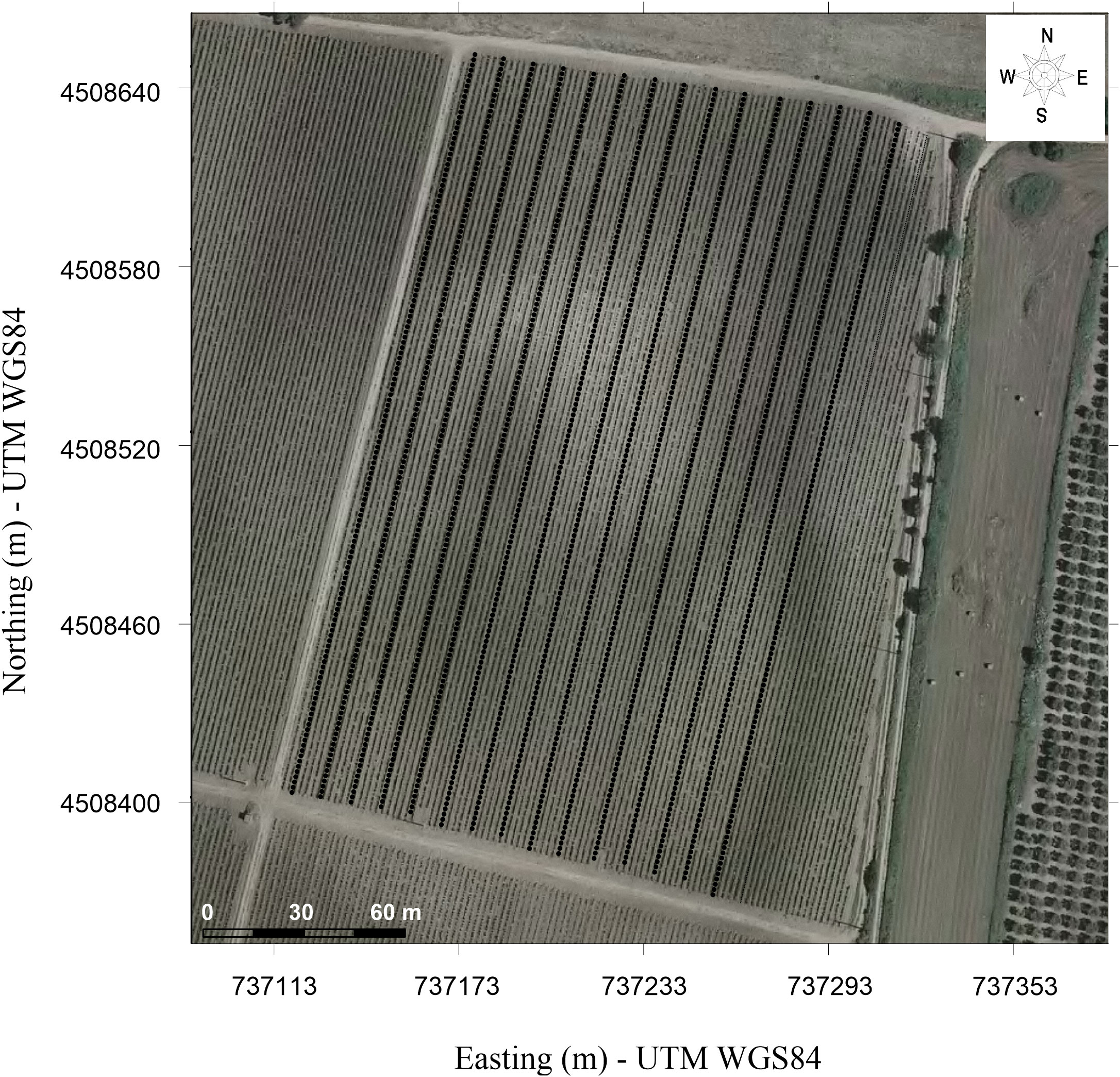
Figure 2 Location of FDEM measurements along n.16 transects. The map coordinates are in WGS84/UTM33N (EPSG:32633).

2.3 EMI data inversion

The ECa data were processed with EM4SOIL code (EMTOMO) to obtain an accurate distribution of the true electrical conductivity, σ. The code uses a nonlinear smoothness-constrained inversion algorithm described in (51, 52) for producing quasi-3D conductivity imaging. A forward modeling subroutine based on the cumulative function (53, 54) is used for solving the EM fields and calculating the theoretical Eca responses at the nodes of a tridimensional mesh of hexahedral blocks distributed according to the locations of the measurement points. The nonlinearity between the model response (log of the apparent electrical conductivity, σ_a) and the model parameters (log of the conductivity of the hexahedral blocks) is solved through the minimization of the objective function defined in Equation 1.

$\begin{array}{ll}\mathit{Q}={\Vert {\mathit{W}}_{\mathit{d}}\mathbf{(}{\mathit{\delta }}_{\mathit{d}}-\mathit{J}{\mathit{\delta }}_{\mathit{p}}\mathbf{)}\Vert }^{\mathbf{2}}+\mathit{\lambda }{\Vert \mathit{C}\mathbf{(}\mathit{p}-{\mathit{p}}_{\mathbf{0}}\mathbf{)}\Vert }^{\mathbf{2}}& (1)\end{array}$

Where W_d is a diagonal matrix, consisting of the reciprocal of data error standard deviations, δ_p is the vector containing the corrections to the model parameters, and p_o is an a priori defined model. The expression δ_d is the vector of the differences between the logarithms of the model responses and the measured data, and J is the derivative matrix (Jacobian) containing the derivatives of the model responses with respect to the model parameters. The parameter λ (also called the damping factor) is a Lagrange multiplier and is used to control the balance between the data fit and the smoothness difference of the model from the a priori model. The elements of the matrix C are coefficients of the roughness value of each parameter (block conductivity), defined in terms of the neighbors (upper, north, south, east, west, and lower blocks).

The earth model used in the inversion process consists of a set of 1D models distributed according to the locations of the measurement points with the thickness of the layers kept constant. An S2 inversion algorithms (55) was applied because it constrains the variation of the parameters around a reference model during inversion by producing smooth models.

Prior to the data inversion, a pre-processing data analysis consisting of a spatial resampling of the six datasets, i.e. the combination of the three depths and two coil configurations, was performed in order to ensure the same number of equally spaced measurement points. This allowed us to set up one single data set containing a series of 5,796 measurement points. Then, the dataset was filtered out by removing some bad data points, typically negative values due to noise or weak induction. A starting homogeneous subsurface was chosen with σ=10 mS m^-1. A Cumulative Function (CF) model (53) and a full solution (FS) model (56) were used to carry out forward modelling, and a damping factor of λ = 0.07 was chosen as the optimal set of inversion parameters.

2.4 Soil moisture

Twenty-four soil samples (P1- P24) were collected at a depth of 0.10 m from the ground level in order to determine the field volumetric soil moisture (VSM) and bulk density and to provide the ground truth for the geophysical signal. The choice of sampling location and depth (red points in Figure 3) was planned according to the EC zoning obtained from the EMI findings.

Figure 3

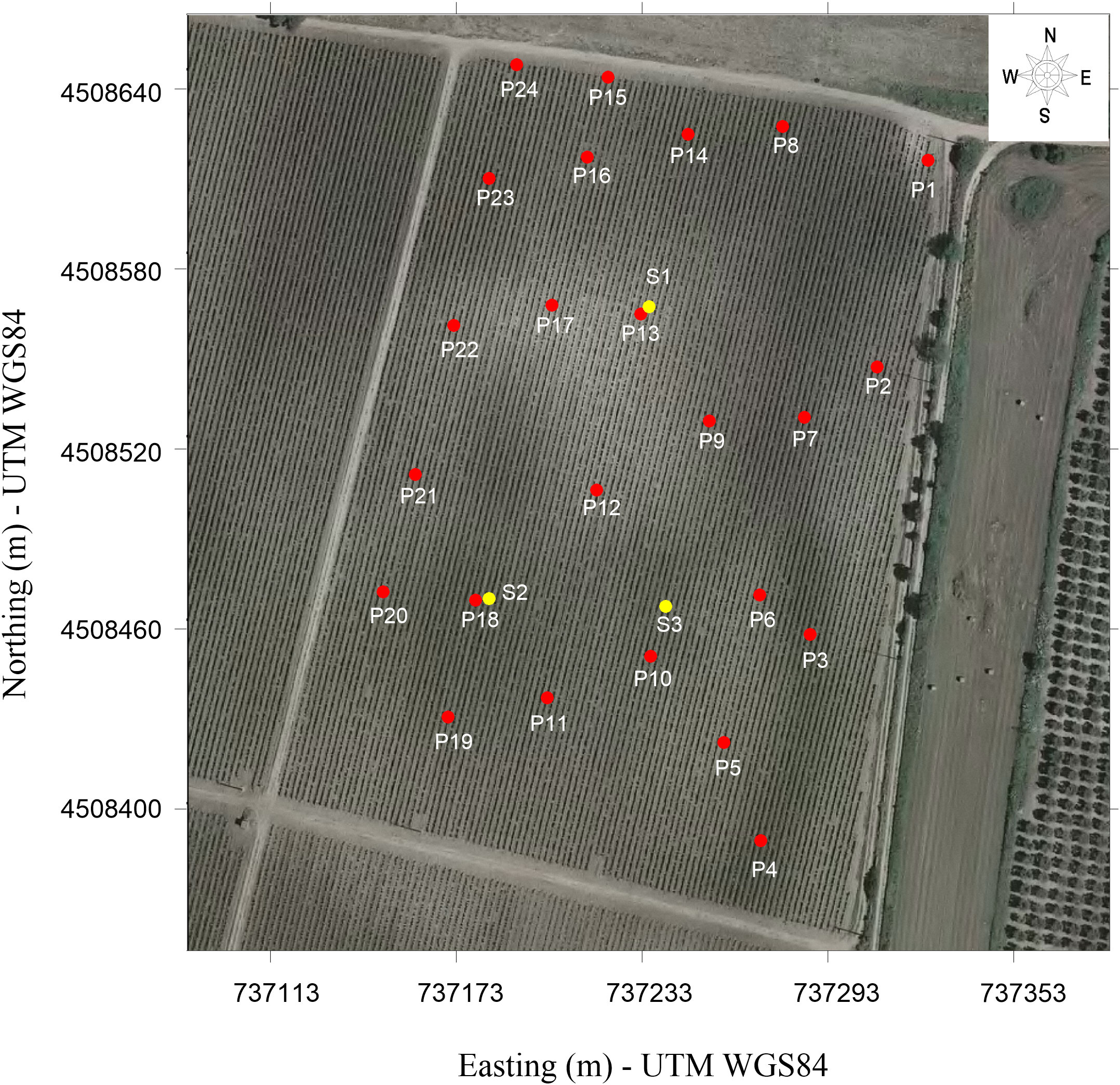
Figure 3 Location of sampling points for determining volumetric soil moisture (red circles from P1 to P24) and GSD analysis (yellow circles from S1 to S3). The map coordinates are in WGS84/UTM33N (EPSG:32633).

The samples were collected directly on site using the Eijkelkamp Sample Ring Kit with an open ring holder which, assembled with each ring, is inserted at a specific depth into the ground by simply turning a handle. The stainless steel rings of known volume were entirely filled with soil. Each ring with soil was weighed using a field scale and the difference between it and the dry weight, obtained in the laboratory by oven drying, allowed us to obtain the volumetric soil moisture for each soil sample collected.

In addition, three soil samples, S1, S2, and S3 in Figure 3, representative of three different EC zones, were collected to determine the grain-size distribution (GSD) in order to associate the EC signal with the soil texture. The GSD was carried out according to the Italian national legislation (57), which requires the use of sieves for analysis of a fraction greater than 2 mm and of a hydrometer for a fraction less than 2 mm.

During the soil sampling, additional point-scale FDEM measurements were collected by setting an RMS error less than 1% in order to define an in-situ empirical calibration function so as to convert the EC data to moisture content. Although ECa does not represent the true soil electrical conductivity, it is reasonable to assume this parameter as representative of the electrical conductivity of the upper soil layer (0−25 cm) comparable with the sampling depth, which is about 10 cm from the ground surface.

2.5 The MoisturEC code

MoisturEC code (58) was used for converting the inverted electrical conductivity (EC) data to soil moisture by capitalizing on the accuracy of the point-scale analysis performed on the soil samples and the huge volume of EC data derived from the FDEM measurements.

The code makes use of the electrical conductivity data and the moisture content values as input, as well as a petrophysical relationship (typically Archie’s law or site specific correlation function) for converting the electrical conductivity data to moisture. The data are weighted based on user inputs and a resolution matrix. In fact, when a measurand, y, is calculated from other measurements through a functional relationship, uncertainties in the input variables will propagate through the calculation to an uncertainty in the output y. MoisturEC code can include all kind of individual error sources as input for the final volumetric soil moisture estimation. Errors can arise from the measurements of volumetric soil moisture on core samples, FDEM original data collected in field, and FDEM data inversion procedure and errors from the petrophysical relationship that relates θ to σ. These errors are carried through the estimation by the standard rules of error propagation, mentioned in (59).

On the other hand, the resolution matrix of the inverse problem defines a linear relationship in which each solution parameter is derived from the weighted averages of nearby true-model parameters, and the resolution matrix elements are the weights. Therefore, the final moisture estimate is obtained by considering all the data and errors to estimate an optimal compromise between data fit and smoothing.

As output, the program yields 2D and 3D images of EC-derived moisture contents obtained by applying an interpolation based on Tikhonov regularization.

Specifically, the moisture contents m at grid nodes are estimated through a linear solution of Equation 2:

$\begin{array}{ll}[{\mathit{J}}^{\mathit{T}}{{\mathit{C}}_{\mathit{D}}}^{-\mathbf{1}}\mathit{J}+\mathit{\alpha }{\mathit{D}}^{\mathit{T}}\mathit{D}]\mathit{m}={\mathit{J}}^{\mathit{T}}{{\mathit{C}}_{\mathit{D}}}^{-\mathbf{1}}\mathit{d}& (2)\end{array}$

where d are the data (volumetric soil moisture from samples and moisture content derived from EC), J is the Jacobian matrix, C_D is the diagonal covariance matrix which consists of the data error variances e, (and C_D^-1 are the data weights), D is the regularization matrix consisting of a first derivative finite-difference filter between adjacent model elements, and α is the tradeoff term that controls the balance between the regularization criteria and data misfit.

In order to decrease the error, the program performs an optimization of the parameter α. An initial estimate of α =1 is used, which indicates an equal weight between smoothing and data misfit. The tradeoff value α is then repeatedly perturbed to find an optimum value for α to compute the final set of model parameters, m. The value of α is achieved through a parabolic interpolation that minimizes an objective function, ϕ Equation 3

$\begin{array}{ll}\mathit{\varphi }={({\mathit{\chi }}^{\mathbf{2}}-\mathbf{1})}^{\mathbf{2}}& (3)\end{array}$

which is informed by a chi-squared statistic, χ². The χ² includes the propagated errors for each EC derived and moisture measurement. Thus, the solution is achieved when the data misfit values are of the same order as the data errors.

In the specific case study, EC data extracted from the quasi-3D model, point scale moisture data derived from the lab analysis, and the calibration data ECa-θ were uploaded as required from the code. Particular attention was devoted to the geophysical and hydrological data error estimation. In the inverted EC data file, an error of 10% was set in order to take into account the model error introduced through inversion, considering that the CMD Mini-Explorer sensor does not provide an estimation of the data error when the continuous acquisition mode is set. On the other hand, an error estimation on the moisture data was set to 1%, by applying Equation 4, i.e., the formula for uncertainty in a function of several variables (60).

$\begin{array}{ll}\begin{array}{ccc}{\sigma }_{{\theta }_v}=\sqrt{{\left(\frac{1}{W_d}{\sigma }_{W_d}\right)}^2+{\left(\frac{W_n}{W_d^2}{\sigma }_{W_d}\right)}^2}& =\sqrt{\frac{1}{W_d^2}{\sigma }_{W_d^2}+\frac{W_n^2}{W_{d^4}}{\sigma }_{W_d^2}}& =\frac{{\sigma }_{W_d}}{W_d}\sqrt{1+\frac{W_n^2}{W_d^2}}\end{array}& (4)\end{array}$

where σ_θv is the measurement error of the volumetric soil moisture of cores, W_d is the dry weight of the core, W_n is the natural weight of the core, and σ_Wd is the error measurements of the W_d and W_n, assumed to be coincident with the repeatability of the balance. In the formula, the value of the volume is assumed with no error.

3 Results

3.1 Soil electromagnetic model

Raw data were preliminarily analyzed for detecting outliers and electromagnetic noise, which usually adversely affect the quality of the inversions. Figure 4 shows the ECa maps for both VCP (4a-c) and HCP (4d-f) coil configurations, respectively. The distribution of ECa highlights some peculiarities about the soil properties: 1) the main variations are located in the upper soil layer (Figure 4A, corresponding to a depth range 0-0.25 m); 2) a significant change in ECa is detected in the depth range of 0.25−0.50 m, although it is not possible to accurately recognize such depth; and 3) differences in the ECa distribution between the VCP and HCP maps are recognized, attributed to the different sensitivity with depth of the two coil configurations. For all these reasons, an inversion process, which takes into account different multi-configuration measurements, sensitivity, and resolution, is needed to include such uncertainties. The FDEM model derived from the inversion process is shown in Figures 5, 6. The EC values range from 5 to 25 mS m^-1, revealing a conductive signal of the investigated soil. The two different visualization modes highlight the main features of the soil properties. Particularly, the 2D cross-sections imaging (Figure 5) detects a sharp soil discontinuity surface which emphasizes a two-layer model: 1) an upper layer that consists of silt and silty loam, as confirmed by GSD analysis and 2) a bottom clayey layer. On the other hand, the 3D perspective visualized in Figure 6 reveals a clear soil heterogeneity in the upper surficial layer. On the base of the geophysical findings, homogeneous EC areas were distinguished (Figure 7) by defining some EC thresholds. Three main zones were identified: 1) a low conductive zone, with values lower than 8 mS m^-1 mainly concentrated in the north-central part and locally in the eastern part of the plot; 2) an intermediate conductive zone, having values between 8 and 16 mS m^-1; and 3) a high conductive zone with values higher than 16 mS m^-1.

Figure 4

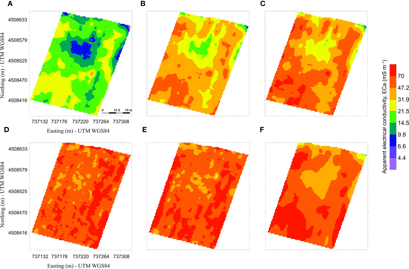
Figure 4 Apparent electrical conductivity (ECa) maps collected with different inter-coil distances and configurations: (A) 0.32 m – vertical coplanar position (VCP); (B) 0.71 m - vertical coplanar position (VCP); (C) 1.18 m - vertical coplanar position (VCP); (D) 0.32 m - horizontal coplanar position (HCP); (E) 0.71 m - horizontal coplanar position (HCP); and (F) 1.18 m - horizontal coplanar position (HCP).

Figure 5

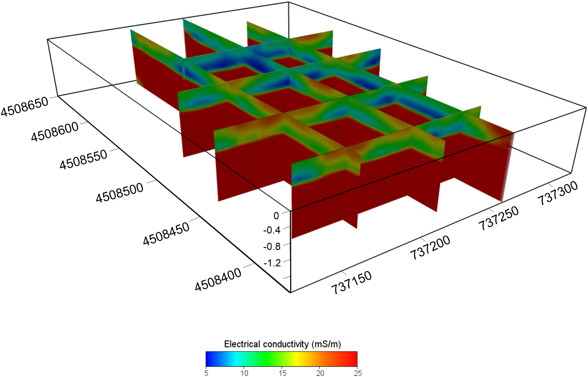
Figure 5 2D cross section extracted from the quasi-3D modeling.

Figure 6

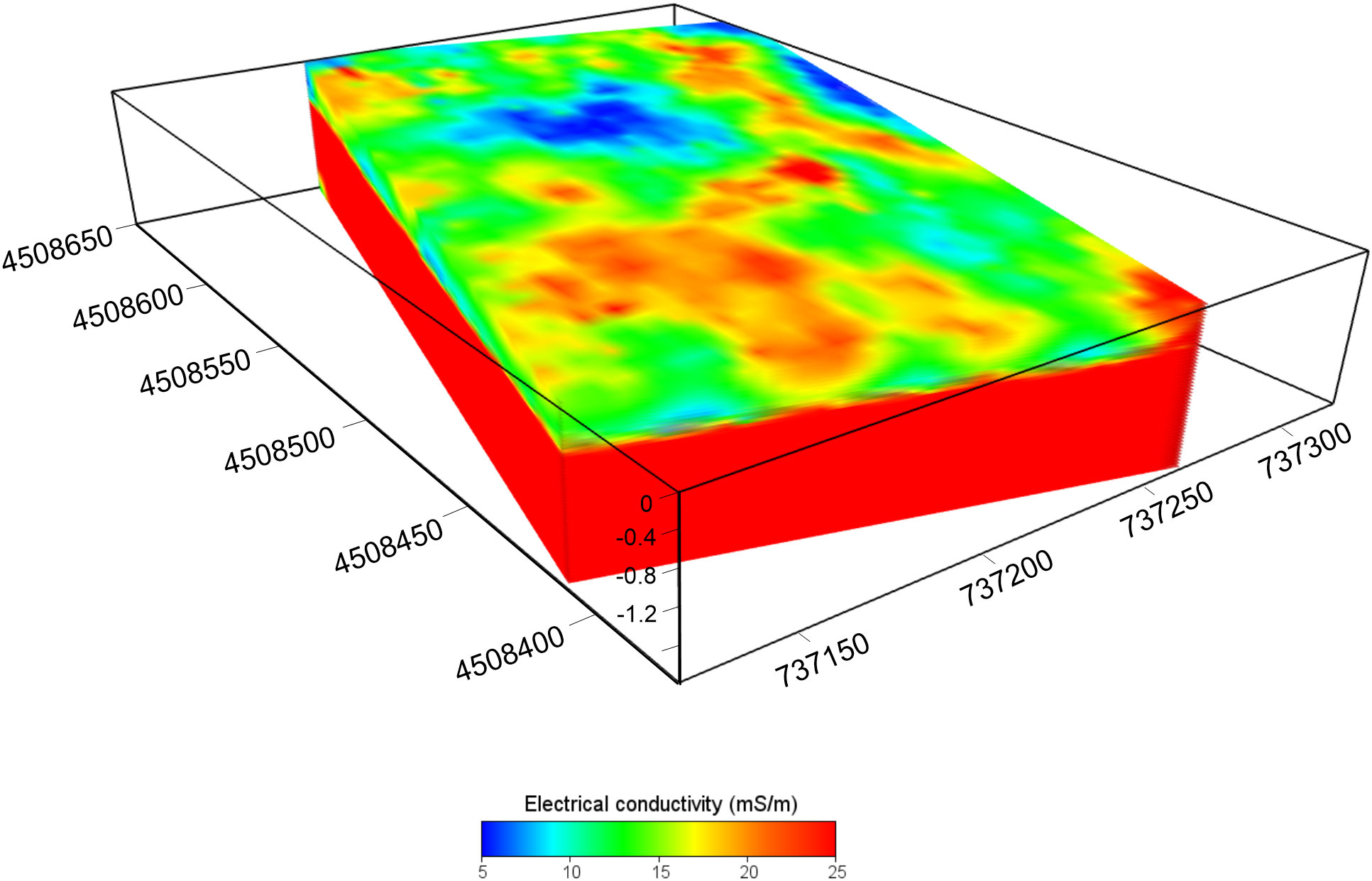
Figure 6 Quasi-3D model obtained from EM4SOIL code.

Figure 7

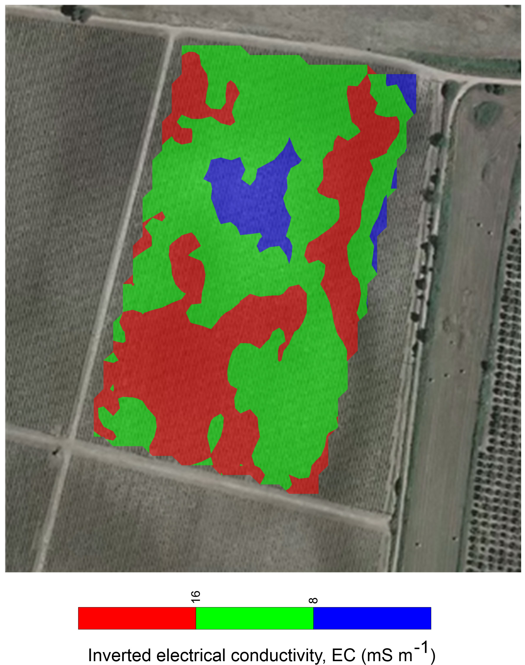
Figure 7 EC zoning extracted from the geophysical model at 0.1 m from ground surface. Blue zone corresponds to low conductive area (EC<8 mS m^-1), green zone to intermediate conductive area (8<EC<16 mS m^-1), and red zone to high conductive area (EC>16 mS m^-1).

3.2 Soil moisture analysis

Table 1 shows the measurements of the bulk density, ρb (g cm^-3), and volumetric soil moisture, θ (m³ m^-3) of the collected soil samples. The soil moisture distribution ranges from 0.21 to 0.37, reflecting the soil heterogeneity shown in the FDEM maps.

Table 1

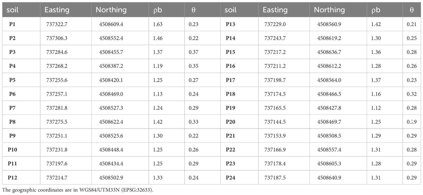
Table 1 Geographical coordinates of sampling points, bulk density, ρb (g cm^-3) and volumetric soil moisture, and θ (m³ m^-3) of collected soil samples from a vineyard in the Carovigno countryside.

The empirical calibration functions used to convert EC data to moisture content are shown in Figure 8. In particular, the VSM_ECa has been compared with the VSM_EC in order to evaluate the best correlation to be used for conversion. A general trend was observed, by confirming the strict correlation between the two parameters (Pearson’s correlation r=0.89 in case of using ECa data and r=0.87 when inverted EC was correlated with VSM). A few pairs of points were removed from both the graphs because they were out of the general trend, probably due to the slightly different volumes of interest of the two kinds of measurements or to the geophysical data noise. In order to evaluate how ECa or inverted EC affect the VSM estimation, the maps obtained with both correlation functions have been produced and compared each other (Figure 9). The maps highlight common patterns but a different VSM range, showing an underestimation of VSM when ECa is used. In accordance with this hypothesis, the comparison between the predicted VSM_ECa (obtained from ECa) and the VSM_EC (obtained from inverted EC) against the measured VSM is visualized in Table 2. The VSM_EC is closer to the measured VSM than the VSM_ECa, above all in correspondence with the high values of measured VSM. This evidence led us to use the inverted data and the calibration function EC vs VSM as input for the MoisturEC code.

Figure 8

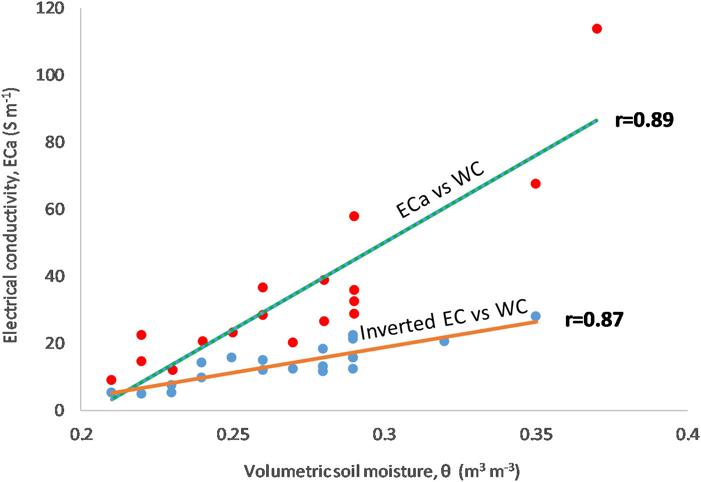
Figure 8 Regression line between ECa and inverted EC vs VSM. ECa data were collected with configuration coil 0.32 m - VCP.

Figure 9

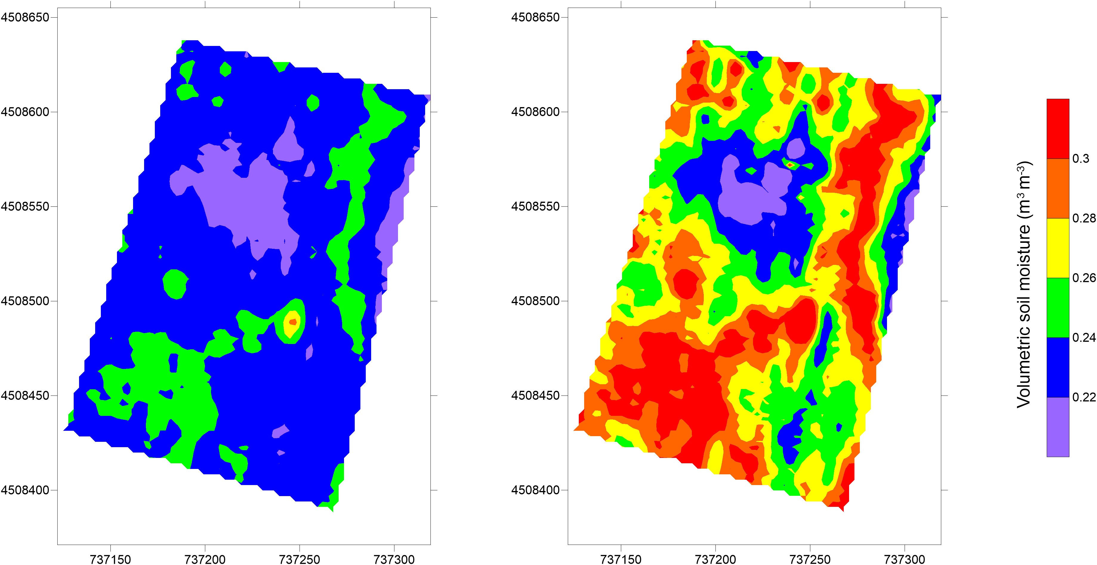
Figure 9 Comparison between volumetric soil moisture predicted from ECa data (left) and inverted EC (right).

Table 2

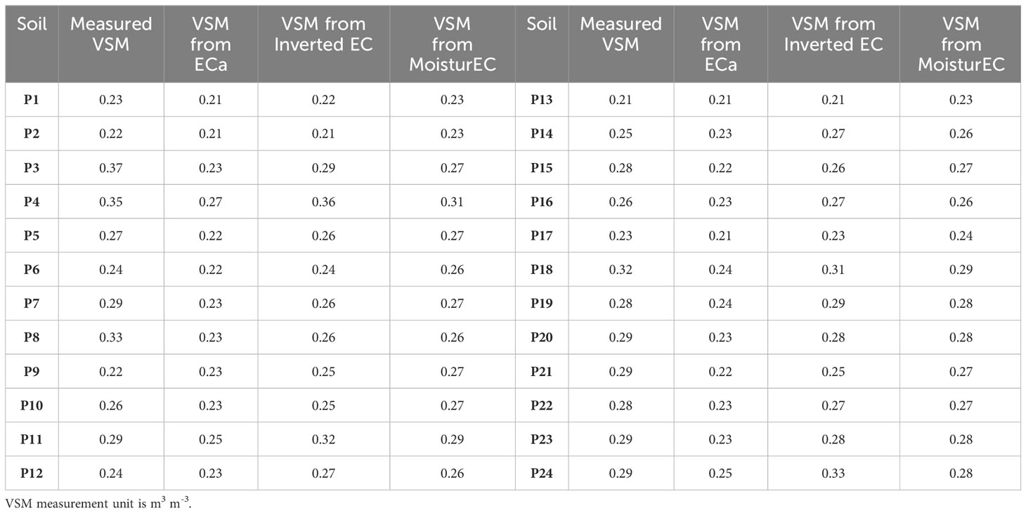
Table 2 Comparison between measured VSM, predicted VSM from ECa, predicted VSM from Inverted EC, and predicted VSM from MoisturEC.

According to the United States Department of Agriculture (USDA) classification (Table 3), S1, S2, and S3 soils were classified as silty loam, silt, and silty loam, respectively, given their percentage of coarse sand (10%, 3%, and 6%), fine sand (12%, 11%, and 14%), coarse silt (62%, 72%, and 66%), fine silt (13%, 12%, and 12%), and clay (3%, 2%, and 2%).

Table 3

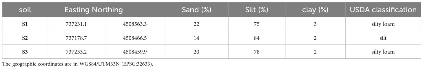
Table 3 Particle-size distribution of the three soil samples corresponding to the S1, S2, and S3 samples.

3.3 Integration between FDEM and soil moisture data

Figures 10, 11 show the soil moisture output from the MoisturEC code in terms of soil moisture estimations and soil moisture error estimation, respectively. The regularization criterion used for calculating the soil moisture provides a smoothness trend in the map. Low values are observed in the central part of the plot, surrounded by areas with higher moisture contents. The map agrees well with the geophysical findings (Figures 4A, 6), as well as with the visual evidence shown in the Google Earth imagery (Figure 3), by confirming a common trend of such observations. The reliability of this approach is corroborated by the low values of the error propagation, which has the same units as the moisture content.

Figure 10

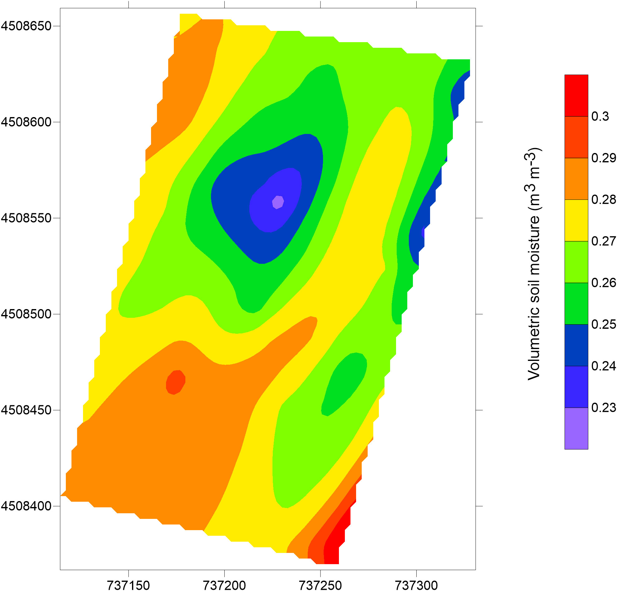
Figure 10 Map of soil moisture distribution obtained through the MoisturEC code.

Figure 11

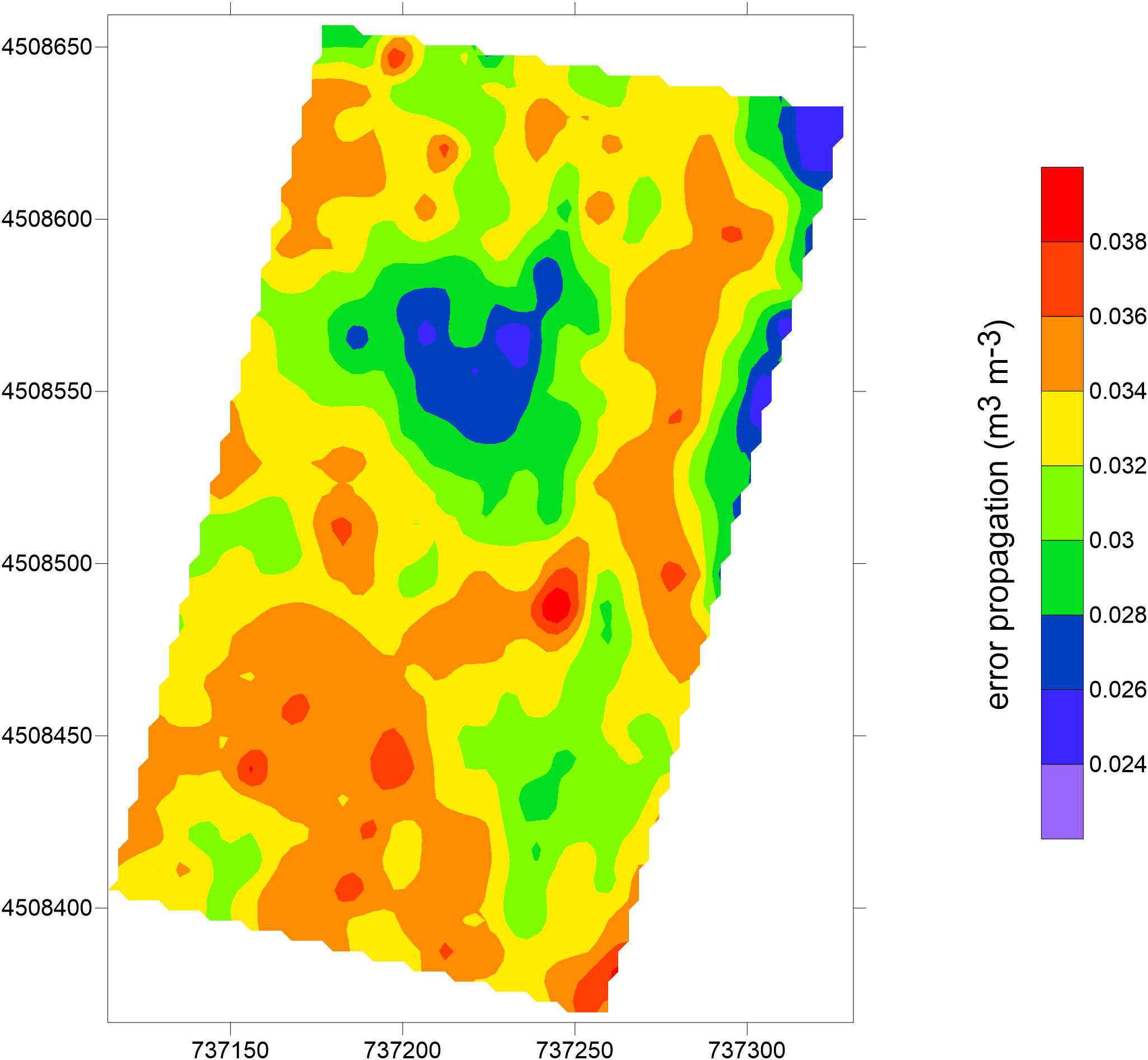
Figure 11 Map of soil moisture error propagation.

4 Discussion

In the last decades, increasing water demand has been posing a serious problem in terms of water availability. To deal with this issue, multi-scale sensors and integrated data analysis tools are needed to produce accurate real-time soil moisture mapping which, in turn, is crucial to assess water availability over time.

We presented a multidisciplinary approach for obtaining soil moisture maps in a vineyard, by combining noninvasive and indirect electromagnetic measurements with traditional soil moisture estimations through soil samples analysis. The integration between such different data types was performed through a data analysis tool, MoisturEC, licensed from USGS, specifically for this purpose. In the scientific landscape, the use of electromagnetic techniques for agricultural purposes has become widespread in the last decades because of the correlation between electrical conductivity and the main soil properties, typically moisture content and salinity. From a geophysical point of view, straightforward approaches based on visualization of the apparent electrical conductivity, ECa, have proved to often be inaccurate in defining a rigorous electromagnetic soil modeling, it being a depth-weighted parameter that gives limited information about the variation of the conductivity with depth. Moreover, the petrophysical correlation functions that are typically used for converting ECa to soil properties are calibrated under very different experimental conditions in terms of spatial scale. In addition, the gap in terms of spatial variability among the dense geophysical data, sparse soil moisture measurements and the intrinsic data, and model uncertainty in the hydrological estimation is a crucial factor that has not been investigated so far.

The presented study aimed to provide a contribution on the use of electromagnetic measurements for estimating reliable volumetric soil moisture, by addressing the aforementioned limitations and shortcomings. The key findings of this study show the capability of the electromagnetic tool to map soil heterogeneities on a large spatial scale. Compared with the raw ECa data, the inversion processing significantly improves the resolution of the soil model by detecting the soil thickness above the bedrock, which cannot be accurately defined with the solely qualitative ECa maps. Figures 4A, 5, 6 clearly highlight the soil heterogeneities concentrated in the upper soil layer. This is reasonable considering the shallow depth of the grape roots zone (thickness about 40-50 cm) and hence the low depth of the soil−water−plant interaction. The soil zoning derived from the geophysical findings (Figure 7) helped in optimizing the soil sampling. Compared to a random sampling scheme, this approach may be essential for ensuring the representativeness of the soil samples. The reliability of the EC zoning is supported by the Google Earth imagery observation (see Figure 2), where the light gray tones correspond to the low conductive zone (blue in the EC zoning). Conversely, the dark gray tones correspond to the green and red areas, which represent the intermediate and the high conductive zones, respectively. The conversion of the ECa and inverted EC data into VSM and their comparison with the measured VSM support the hypothesis that the inverted data are more consistent than raw ECa data, strengthening the importance of the inversion process, in addition to the aforementioned considerations. This is clearly visualized in Table 2, where the comparison between the predicted VSM_ECa and VSM_EC against measured VSM is observed. Since the direct use of site-specific calibration functions can lead to potential artifacts or unrealistic estimations, a quantitative integration of invasive and non-invasive soil information has been performed using a straightforward software tool, MoistureEC code, which considers the error distribution of both datasets in the VSM estimation. Table 2 also includes the predictions of VSM from MoisturEC inferred from the 2D map (Figure 10). In general, the output of the code reflects the soil heterogeneities in terms of soil texture: lower values correspond to the areas with a higher percentage of sand and higher values are recorded in the silty soil. This assumption is confirmed by the GSD analysis and the moisture estimation of the soil samples. In fact, the textural soil properties affect the geophysical and the hydrological response, as expected. The higher percentage of sand found in the S1 sample is consistent with the lower moisture content measured near the soil sample P13. Conversely, the silty fraction in the S2 and S3 samples, which retains more water than sand, provides higher moisture content near the soil samples P18 and P16.

In detail, MoisturEC code provided more accurate VSM estimations than the predictions obtained through the inverted EC, although some deviations from measured VSM have been recorded at a few points. In particular, the model underestimates the high conductivity values, with particular reference to the portion between P7 and P8, probably due to the lack of soil sampling points in that area. In addition, the difference in the data error weight between the field scale geophysical data (error estimation set to 10%) and point soil moisture measurements (1%) makes these latter data predominant in the final result. This is a crucial point concerning the use of such geophysical measurements for providing quantitative estimation of the investigated soil. In fact, maintaining high quality data is essential for converting geophysical data to hydrological data. These findings suggest future research to improve the geophysical outputs by reducing the model error, which, in turn, depends on the data error. Collecting electromagnetic data in a manual mode by setting a low standard deviation error, which is not possible with the continuous measurement. mode, allows accurate checking of the measurement error. Regardless, the low values of error propagation ranging from 0.03 to 0.05 m³ m^-3 (Figure 11) corroborate the reliability of such an integrated approach to moisture estimation. Overall, this study showed the reliability of the contactless electromagnetic approach for soil investigation, by confirming the great potentialities and benefit for agricultural purposes. This approach can be routinely used in the agricultural field in order to better understand the spatio-temporal hydrological dynamics and support the predictive modeling of the spatio-temporal dynamics of the soil−water−plant system.

Data availability statement

The raw data supporting the conclusions of this article will be made available by the authors, without undue reservation.

Author contributions

LD: Writing – original draft, Conceptualization, Data curation, Formal Analysis, Investigation, Methodology. AT: Writing – review & editing, Data curation, Investigation, Validation, Visualization. MC: Writing – review & editing, Data curation, Investigation, Supervision, Validation, Visualization.

Funding

The author(s) declare financial support was received for the research, authorship, and/or publication of this article. Part of the research activities proposed in this paper were developed within the INTER-ACTION project, awarded by the Belmont Forum, in the framework of the call for a Collaborative Research Action (CRA) on the theme Towards Sustainability of Soils and Groundwater for Society and supported through a Belmont Forum (Earth System Science and Environmental Technologies Department of the National Research Council of Italy) grant (Belmont forum-CNR: B55F21001250007) (https://belmontforum.org/projects?fwp_project_call=soils2020, accessed on November 2nd 2023).

Acknowledgments

The authors wish to thank Greco Farm, owner of the vineyard, for making the experimental plot facility available to carry out the experimental activities concerning FDEM measurements and soil sampling. A special mention to Domenico Bellifemine for his contribution in the technical aspects.

Conflict of interest

The authors declare that the research was conducted in the absence of any commercial or financial relationships that could be construed as a potential conflict of interest.

The handling editor MF declared a past co-authors ship with the authors.

Publisher’s note

All claims expressed in this article are solely those of the authors and do not necessarily represent those of their affiliated organizations, or those of the publisher, the editors and the reviewers. Any product that may be evaluated in this article, or claim that may be made by its manufacturer, is not guaranteed or endorsed by the publisher.

References

1. Friedman SP. Soil properties influencing apparent electrical conductivity: a review. Comput Electron Agr (2005) 46:45–70. doi: 10.1016/j.compag.2004.11.001

CrossRef Full Text | Google Scholar

2. Weymer BA, Everett ME, de Smet TS, Houser C. Review of electromagnetic induction for mapping barrier island framework geology. Sediment Geol (2015) 321:11–24. doi: 10.1016/j.sedgeo.2015.03.005

CrossRef Full Text | Google Scholar

3. Paepen M, Hanssens D, De Smedt P, Walraevens K, Hermans T. Combining resistivity and frequency domain electromagnetic methods to investigate submarine groundwater discharge in the littoral zone. Hydrol Earth Syst Sci (2020) 24:3539–55. doi: 10.5194/hess-24-3539-2020

CrossRef Full Text | Google Scholar

4. McLachlan P, Blanchy G, Chambers J, Sorensen J, Uhlemann S, Wilkinson P, et al. The application of electromagnetic induction methods to reveal the hydrogeological structure of a riparian wetland. Water Resour Res (2021) 57:e2020WR029221. doi: 10.1029/2020WR029221

CrossRef Full Text | Google Scholar

5. Deidda GP, De Carlo L, Caputo MC, Cassiani G. Frequency domain electromagnetic induction imaging: An effective method to see inside a capped landfill. Waste Manage (2022) 144:29–40. doi: 10.1016/j.wasman.2022.03.007

CrossRef Full Text | Google Scholar

6. Corwin DL, Lesch SM. Apparent soil electrical conductivity measurements in agriculture. Comput Electron Agr (2005) 46:11–43. doi: 10.1016/j.compag.2004.10.005

CrossRef Full Text | Google Scholar

7. Doolittle JA, Brevik EC. The use of electromagnetic induction techniques in soils studies. Geoderma (2014) 223-225:33–45. doi: 10.1016/j.geoderma.2014.01.027

CrossRef Full Text | Google Scholar

8. Rodrıguez-Perez JR, Plant RE, Lambert JJ, Smart DR. Using apparent soil electrical conductivity (ECa) to characterize vineyard soils of high clay content. Precis Agric (2011) 12:775–94. doi: 10.1007/s11119-011-9220-y

CrossRef Full Text | Google Scholar

9. Martini E, Werban U, Zacharias S, Pohle M, Dietrich P, Wollschläger U. Repeated electromagnetic induction measurements for mapping soil moisture at the field scale: validation with data from a wireless soil moisture monitoring network. Hydrol Earth Syst Sci Discuss (2016) 21:495–513. doi: 10.5194/hess-2016-93

CrossRef Full Text | Google Scholar

10. Yao R, Yang J, Wu D, Xie W, Gao P, Jin W. Digital mapping of soil salinity and crop yield across a coastal agricultural landscape using repeated electromagnetic induction (EMI) surveys. PloS One (2016) 11(5):e0153377. doi: 10.1371/journal.pone.0153377

PubMed Abstract | CrossRef Full Text | Google Scholar

11. Käthner J, Ben-Gal A, Gebbers R, Peeters A, Herppich WB, Zude-Sasse M. Evaluating spatially resolved influence of soil and tree water status on quality of european plum grown in semi-humid climate. Front Plant Sci (2017) 8:1053. doi: 10.3389/fpls.2017.01053

PubMed Abstract | CrossRef Full Text | Google Scholar

12. Scudiero E, Skaggs TH, Corwin DL. Simplifying field-scale assessment of spatiotemporal changes of soil salinity. Sci Total Environ (2017) 587–588:273–81. doi: 10.1016/j.scitotenv.2017.02.136

PubMed Abstract | CrossRef Full Text | Google Scholar

13. Singh J, Loa T, Rudnick DR, Dorr TJ, Burr CA, Werle R, et al. Performance assessment of factory and field calibrations for electromagnetic sensors in a loam soil. Agr Water Manage (2018) 196:87–98. doi: 10.1016/j.agwat.2017.10.020

CrossRef Full Text | Google Scholar

14. Blanchy G, Watts CW, Ashton RW, Webster CP, Hawkesford MJ, Whalley WR, et al. Accounting for heterogeneity in the ϑ-σ relationship: Application to wheat phenotyping using EMI. Vadose Zone J (2020) 19:e20037. doi: 10.1002/vzj2.20037

CrossRef Full Text | Google Scholar

15. Brillante L, Martínez-Lüscher J, Yu R, Kurtural SK. Carbon isotope discrimination (13C) of grape musts is a reliable tool for zoning and the physiological ground-truthing of sensor maps in precision viticulture. Front Environ Sci (2020) 8:561477. doi: 10.3389/fenvs.2020.561477

CrossRef Full Text | Google Scholar

16. Cursi DE, Gazaffi R, Hoffmann HP, Brasco TL, do Amaral LR, Dourado Neto D. Novel tools for adjusting spatial variability in the early sugarcane breeding stage. Front Plant Sci (2021) 12:749533. doi: 10.3389/fpls.2021.749533

PubMed Abstract | CrossRef Full Text | Google Scholar

17. Yu R, Zaccaria D, Kisekka I, Kurtural SK. Soil apparent electrical conductivity and must carbon isotope ratio provide indication of plant water status in wine grape vineyards. Precis Agric (2021) 22:1333–52. doi: 10.1007/s11119-021-09787-x

CrossRef Full Text | Google Scholar

18. Hubbard SS, Schmutz M, Balde A, Falco N, Peruzzo L, Dafflon B, et al. Estimation of soil classes and their relationship to grapevine vigor in a Bordeaux vineyard: advancing the practical joint use of electromagnetic induction (EMI) and NDVI datasets for precision viticulture. Precis Agric (2021) 22:1353–76. doi: 10.1007/s11119-021-09788-w

CrossRef Full Text | Google Scholar

19. De Carlo L, Vivaldi GA, Caputo MC. Electromagnetic induction measurements for investigating soil salinization caused by saline reclaimed water. Atmosphere (2022) 13:73. doi: 10.3390/atmos13010073

CrossRef Full Text | Google Scholar

20. Emmanuel ED, Lenhart CF, Weintraub MN, Doro KO. Estimating soil properties distribution at a restored wetland using electromagnetic imaging and limited soil core samples. Wetlands (2023) 43:39. doi: 10.1007/s13157-023-01686-3

CrossRef Full Text | Google Scholar

21. Brown M, Heinse R, Johnson-Maynard J, Huggins D. Time-lapse mapping of crop and tillage interactions with soil water using electromagnetic induction. Vadose Zone J (2021) 20:e20097. doi: 10.1002/vzj2.20097

CrossRef Full Text | Google Scholar

22. Pedrera-Parrilla A, Van De Vijver E, Van Meirvenne M, Espejo A, Giraldez J, Vanderlinden K. Apparent electrical conductivity measurements in an olive orchard under wet and dry soil conditions: significance for clay and soil water content mapping. Precis Agric (2016) 17:531–45. doi: 10.1007/s11119-016-9435-z

CrossRef Full Text | Google Scholar

23. Martinez G, Vanderlinden K, Giraldez J, Espejo A, Muriel J. Field-scale soil moisture pattern mapping using electromagnetic induction. Vadose Zone J (2010) 9:871 881. doi: 10.2136/vzj2009.0160

CrossRef Full Text | Google Scholar

24. Longo M, Piccoli I, Minasny B, Morari F. Soil apparent electrical conductivity-directed sampling design for advancing soil characterization in agricultural fields. Vadose Zone J (2020) 19:e20060. doi: 10.1002/vzj2.20060

CrossRef Full Text | Google Scholar

25. Bronson KF, Booker JD, Officer SJ, Lascano RJ, Maas SJ, Searcy SW, et al. Apparent electrical conductivity, soil properties and spatial covariance in the U. S. South High Plains. Precis Agric (2005) 6:297–311. doi: 10.1007/s11119-005-1388-6

CrossRef Full Text | Google Scholar

26. Chtouki M, Nguyen F, Garré S, Oukarroum A. Optimizing phosphorus fertigation management zones using electromagnetic induction, soil properties, and crop yield data under semi-arid conditions. Environ Sci pollut Res (2023) 30:106083–98. doi: 10.1007/s11356-023-29658-4

CrossRef Full Text | Google Scholar

27. Barca E, Castrignanò A, Buttafuoco G, De Benedetto D, Passarella G. Integration of electromagnetic induction sensor data in soil sampling scheme optimization using simulated annealing. Environ Monit Assess (2015) 187:1–12. doi: 10.1007/s10661-015-4570-y

PubMed Abstract | CrossRef Full Text | Google Scholar

28. Monteiro Santos F, Triantafilis J, Bruzgulis K. A spatially constrained 1D inversion algorithm for quasi-3D conductivity imaging: application to DUALEM-421 data collected in a riverine plain. Geophysics (2011) 76:B43–53. doi: 10.1190/1.3537834

CrossRef Full Text | Google Scholar

29. Von Hebel C, Rudolph S, Mester A, Huisman JA, Kumbhar P, Vereecken H, et al. Three-dimensional imaging of subsurface structural patterns using quantitative large-scale multiconfiguration electromagnetic induction data. Water Resour Res (2014) 50:2732–48. doi: 10.1002/2013WR014864

CrossRef Full Text | Google Scholar

30. Farzamian M, Autovino D, Basile A, De Mascellis R, Dragonetti G, Monteiro Santos F, et al. Assessing the dynamics of soil salinity with time-lapse inversion of electromagnetic data guided by hydrological modelling. Hydrol Earth Syst Sci (2021) 25:1509–27. doi: 10.5194/hess-25-1509-2021

CrossRef Full Text | Google Scholar

31. Jadoon KZ, Altaf MU, McCabe MF, Hoteit I, Muhammad N, Moghadas D, et al. Inferring soil salinity in a drip irrigation system from multi-configuration EMI measurements using adaptive Markov chain Monte Carlo. Hydrol Earth Syst Sci (2017) 21:5375–83. doi: 10.5194/hess-21-5375-2017

CrossRef Full Text | Google Scholar

32. Moghadas D, Jadoon KZ, McCabe MF. Spatiotemporal monitoring of soil water content profiles in an irrigated field using probabilistic inversion of time-lapse EMI data. Adv Water Resour (2017) 110:238–48. doi: 10.1016/j.advwatres.2017.10.019

CrossRef Full Text | Google Scholar

33. Boico VF, Therrien R, Højberg AL, Iversen BV, Koganti T, Varvaris I. Using depth specific electrical conductivity estimates to improve hydrological simulations in a heterogeneous tile-drained field. J Hydrol (2022) 64:127232. doi: 10.1016/j.jhydrol.2021.127232

CrossRef Full Text | Google Scholar

34. Carrera A, Longo M, Piccoli I, Mary B, Cassiani G, Morari F. Electro-magnetic geophysical dynamics under conservation and conventional farming. Remote Sens (2022) . 14:6243. doi: 10.3390/rs14246243

CrossRef Full Text | Google Scholar

35. Dragonetti G, Farzamian M, Basile A, Monteiro Santos F, Coppola A. In situ estimation of soil hydraulic and hydrodispersive properties by inversion of electromagnetic induction measurements and soil hydrological modeling. Hydrol Earth Syst Sci (2022) 26:5119–36. doi: 10.5194/hess-26-5119-2022

CrossRef Full Text | Google Scholar

36. Dafflon B, Hubbard SS, Ulrich C, Peterson JE. Electrical conductivity imaging of active layer and permafrost in an arctic ecosystem, through advanced inversion of electromagnetic induction data. Vadose Zone J (2013) 12:1–19. doi: 10.2136/vzj2012.0161

CrossRef Full Text | Google Scholar

37. Callegary JB, Ferré TPA, Groom RW. Three-dimensional sensitivity distribution and sample volume of low-induction-number electromagnetic-induction instruments. Soil Sci Soc Am J (2012) 76:85–91. doi: 10.2136/sssaj2011.0003

CrossRef Full Text | Google Scholar

38. Guillemoteau J, Christensen NB, Jacobsen BH, Tronicke J. Fast 3D multichannel deconvolution of electromagnetic induction loop-loop apparent conductivity data sets acquired at low induction numbers. Geophysics (2017) 82:1ND–Z46. doi: 10.1190/geo2016-0518.1

CrossRef Full Text | Google Scholar

39. Hendrickx JMH, Borchers B, Corwin DL, Lesch SM, Hilgendorf AC, Schlue J. Inversion of soil conductivity profiles from electromagnetic induction measurements: theory and experimental verification. Soil Sci Soc Am J (2002) 66:673–85. doi: 10.2136/sssaj2002.6730

CrossRef Full Text | Google Scholar

40. Jadoon KZ, Moghadas D, Jadoon A, Missimer TM, Al-Mashharawi SK, McCabe MF. Estimation of soil salinity in a drip irrigation system by using joint inversion of multicoil electromagnetic induction measurements. Water Resour Res (2015) 51:3490–504. doi: 10.1002/2014WR016245

CrossRef Full Text | Google Scholar

41. von Hebel C, van der Kruk J, Huisman JA, Mester A, Altdor D, Endres AL, et al. Calibration, conversion, and quantitative multi-layer inversion of multi-coil rigid-boom electromagnetic induction data. Sensors (2019) 19:4753. doi: 10.3390/s19214753

PubMed Abstract | CrossRef Full Text | Google Scholar

42. Shanahan PW, Binley A, Whalley WR, Watts CW. The use of electromagnetic induction to monitor changes in soil moisture profiles beneath different wheat genotypes. Soil Sci Soc Am J (2015) 79:459–66. doi: 10.2136/sssaj2014.09.0360

CrossRef Full Text | Google Scholar

43. Pellerin L, Wannamaker PE. Multi-dimensional electromagnetic modeling and inversion with application to near-surface earth investigations. Comput Electron Agr (2005) 46:71–102. doi: 10.1016/j.compag.2004.11.017

CrossRef Full Text | Google Scholar

44. Farzamian M, Bouksila F, Paz AM, Monteiro Santos F, Zemni N, Slama F, et al. Landscape-scale mapping of soil salinity with multi-height electromagnetic induction and quasi-3d inversion in Saharan Oasis, Tunisia. Agr Water Manage (2023) 284:108330. doi: 10.1016/j.agwat.2023.108330

CrossRef Full Text | Google Scholar

45. Tikhonov AN, Arsenin VY. Solutions of Ill Posed Problems. New York: Winston (1977). p. 258.

Google Scholar

46. McKenna SA, Poeter EP. Field example of data fusion in site characterization. Water Resour Res (1995) 31:3229–40. doi: 10.1029/95WR02573

CrossRef Full Text | Google Scholar

47. Archie GE. The electrical resistivity log as an aid in determining some reservoir characteristics. Trans (1942) 146:54–62. doi: 10.2118/942054-G

CrossRef Full Text | Google Scholar

48. Topp GG, Davis JL, Annan AP. Electromagnetic determination of soil water content measurements in coaxial transmission lines. Water Resour Res (1980) 16:574–82. doi: 10.1029/WR016i003p00574

CrossRef Full Text | Google Scholar

49. Birchak JR, Gardner CG, Hipp JE, Victor JM. High dielectric constant microwave probes for sensing soil moisture. Proc IEEE (1974) 62(1):93–8. doi: 10.1109/PROC.1974.9388

CrossRef Full Text | Google Scholar

50. Instruments s.r.o. GF. Short guide for electromagnetic conductivity mapping and tomography (2016). Available at: http://www.gfinstruments.cz/version_cz/downloads/CMD_Short_guide_Electromagnetic_conductivity_mapping-20-04-2020.pdf.

Google Scholar

51. Monteiro Santos FA. 1-D laterally constrained inversion of EM34 profiling data. J Appl Geophys (2004) 56:123–34. doi: 10.1016/j.jappgeo.2004.04.005

CrossRef Full Text | Google Scholar

52. Monteiro Santos FA, Matias H, Goncalves R. The use of the EM34 in cave detection technique. Eur J Environ Eng Geophysics (2001) 6:153–66.

Google Scholar

53. McNeill JD. Electromagnetic terrain conductivity measurement at low induction numbers: Geonics, Technical Note TN-6 (1980). Available at: http://www.geonics.com/pdfs/technicalnotes/tn6.pdf.

Google Scholar

54. Wait JR. A note on the electromagnetic response of a stratified earth. Geophysics (1962) 27:382–5. doi: 10.1190/1.1439028

CrossRef Full Text | Google Scholar

55. Sasaki Y. Full 3-D inversion of electromagnetic data on PC. J Appl Geophysics. (2001) 46:45–54. doi: 10.1016/S0926-9851(00)00038-0

CrossRef Full Text | Google Scholar

56. Monteiro Santos F, Triantafilis J, Bruzgulis K, Roe J. Inversion of multiconfiguration electromagnetic (DUALEM-421S) profiling data using a one-dimensional laterally constrained algorithm. Vadose Zone J (2010) 9:117–25. doi: 10.2136/vzj2009.0088

CrossRef Full Text | Google Scholar

57. D.M. 13 settembre 1999. Decreto Ministeriale 13 settembre 1999, n. 185 “Metodi ufficiali di analisi chimica del suolo”. Gazzetta Ufficiale n. 248 del 21 ottobre 1999 – S.O. n.185 . Available at: https://www.gazzettaufficiale.it/eli/id/1999/10/21/099A8497/sg (Accessed August 15, 2023).

Google Scholar

58. Terry N, Day-Lewis FD, Werkema D, Lane JW. MoisturEC: A new R program for moisture content estimation from electrical conductivity data. Groundwater (2018) 56:823–31. doi: 10.1111/gwat.12650

CrossRef Full Text | Google Scholar

59. Farrance I, Frenkel R. Uncertainty of measurement: A review of the rules for calculating uncertainty components through functional relationships. Clin Biochem Rev (2012) 33:49–75.

PubMed Abstract | Google Scholar

60. Taylor JR. An Introduction to Error Analysis: The Study of Uncertainties in Physical Measurements. New York: University Science Books (1997). p. 327.

Google Scholar