Improving a regional peat thickness map using soil apparent electrical conductivity measurements at the field-scale

1 Introduction

Global peat mapping efforts are driven by the need to determine a peatland’s extent or cover type; generate peat thickness maps to support C stock calculation; inform on potential GHG emissions; and support soil conservation practices (1, 2). The latter is a need often associated with drained and cultivated peatlands. No longer being in anoxic conditions limiting organic matter decomposition, they are subject to degradation of soil chemical and physical properties and soil loss (3–5). Local soil conservation interventions could help prevent a significant decrease in soil productivity, and is therefore essential to feeding the growing population. Many researchers and policymakers are actively working on peatland conservation to ensure their sustainable use and to limit their contribution to climate change; for instance, initiatives have emerged in Canada (6, 7), Europe (8, 9), and globally (10–12). However, large scale soil conservation practices can be costly. Hence, forming priority management zones at the field-scale can be helpful if prior knowledge of soil productivity, degradation level, and long-term potential exists. These activities generally require soil sampling, data processing and analyses, and mapping efforts.

Recently, peat thickness maps were proposed as a tool for monitoring soil degradation and for defining management zones (13, 14). This approach also considered the presence of another organic layer, sometimes found between peaty and mineral layers: the gyttja or limnic layer. This gelatinous material has been described in many soil classification systems (15–19) but is seldom mapped at a regional-scale (20, 21). In an agricultural context, this layer can pose management problems to the farmer due to its high salinity, imperviousness, and reduced drainage capacity when found close to the surface (3, 13). When growing crops, such as leafy vegetables, potatoes, carrots, and onions, the issues caused by limnic layers may be problematic, and sometimes not cultivable, and hence, there is a need to better its spatial distribution. Therefore, efforts to map organic soils, with the presence of limnic layers, should either differentiate peaty, limnic, and mineral layers; or only map the peaty layer. The maximum peat thickness (MPT), or the non-limnic peat thickness, was suggested to reflect the real cultivable layer (13). Beyond the importance of this data for agricultural purposes, distinguishing between peat and limnic layers could lead to more accurate carbon (C) stock estimates given their different chemical nature (21, 22). Finally, knowing the peat thickness with respect to the boundary with the underlying impervious material (limnic or mineral layer) is critical for applying accurate drainage simulations to generate drainage recommendations.

A first attempt to map the MPT at a regional-scale yielded a model with low accuracy and a poor understanding of the drivers of the occurence of limnic layers in soils (14). In their study, Deragon et al. (14) used only remote sensing covariates and trained a model to predict the depth to the mineral layer, and another model to predict the limnic layer thickness. Both maps were then combined to obtain the MPT, resulting in a propagation of errors in the final map. They recommended a field-scale approach, as accuracy improvements was expected with covariates that could better capture the fine-scale variability and ultimately, the spatial variability of the limnic layer. The simplest alternative could be manual sampling; however, it becomes increasingly cost-prohibitive at the farm scale or for larger extents given the time and labour required. Moreover, limnic layers can be difficult to detect with manual probing since the probe offers little resistance to its insertion (14, 23). Furthermore, cultivated organic soils undergo constant degradation and soil loss, increasing the need for temporal monitoring and mapping efforts to update them (24).

Therefore, to reduce the need for manual sampling, field-scale approaches may leverage technologies, such as proximal sensors. These instruments are sensitive to differences in the geoelectrical properties of soil layers. They include apparent electrical conductivity, apparent dielectric permittivity, and gamma-ray emissions for instance, and can differentiate peat from mineral layers given their different signature (1). Examples of proximal geophysical sensors used in peat mapping studies include ground penetrating radars [GPR, e.g., (23, 25–31)], electromagnetic induction [EMI, (32–36)], electrical resistivity tomography (27, 28, 30, 31, 34, 35, 37) and gamma radiometric sensors (36, 38–43). These instruments were used at multiple spatial scales due to their compatibility with various platforms, such as drones, land vehicles and airborne surveys. Many studies have already mapped peatlands or shallow organic deposits at the field scale using one or multiple instruments (28, 33, 43–47), but detecting and reporting limnic layers has rarely been a research objective. Proximal sensors rapidly provide a high density of data and reduce the need for laboratory analyses. In the case of the Montérégie region, Canada, where a regional map of the MPT was generated (14), there is the potential to downscale (i.e., increasing its spatial resolution) such map products by supplementing them with field-scale data and take advantage of previous mapping efforts. To reduce the propagation of error, the need for manual sampling, and improve the prediction accuracies, it is hypothesized that directly predicting the MPT at the field-scale will yield better results compared to the existing regional map. As such, this study had the following objectives: (1) to compare mapping products at field-scale derived from proximal sensor data to a regional map; (2) to test if using the regional map as a covariate can improve the result (i.e, downscaling); and (3) to determine if the covariates can accurately detect the boundary between peat-limnic and peat-mineral layers.

2 Materials and methods

2.1 Study area and soil data collection

A commercial 6.9 ha field, a drained and cultivated organic soil in the Montérégie region, Québec, Canada was selected to investigate the spatial variability of limnic and mineral layers near the soil surface. Ground truth measurements were obtained in May and October 2021. The study area is in a temperate continental/humid continental climate zone, receiving around 970 mm of precipitation per year, while the average temperature is 6.7°C. In May, the average temperature and rainfall are 13.3°C and 91 mm, respectively. Soil cores were extracted at 61 locations in the field using a Macauley sample (Eijkelkamp peat sampler) to a maximum depth of 1.5 m, whereby the depth to the limnic layer was recorded. The sampling design was a 26 m x 36 m rectangular grid with duplicates at some sites to ensure a better representation of the small-scale variability. The dataset should have included an additional seven observations, however, they were removed from the dataset due to the peat deposits being >1.5 m could not be adequately measured with our equipment. This led to a gap in the sampling grid Figure 1. On average, the thickness of the observed limnic layer was 0.28 m (± 0.17 m), with some locations having no limnic layers. The peat soils were classified as an Orthic Humic Gleysol in the shallowest part of the field and transitioned to a Humic Mesisol where the peat accumulation was greater (19).

FIGURE 1

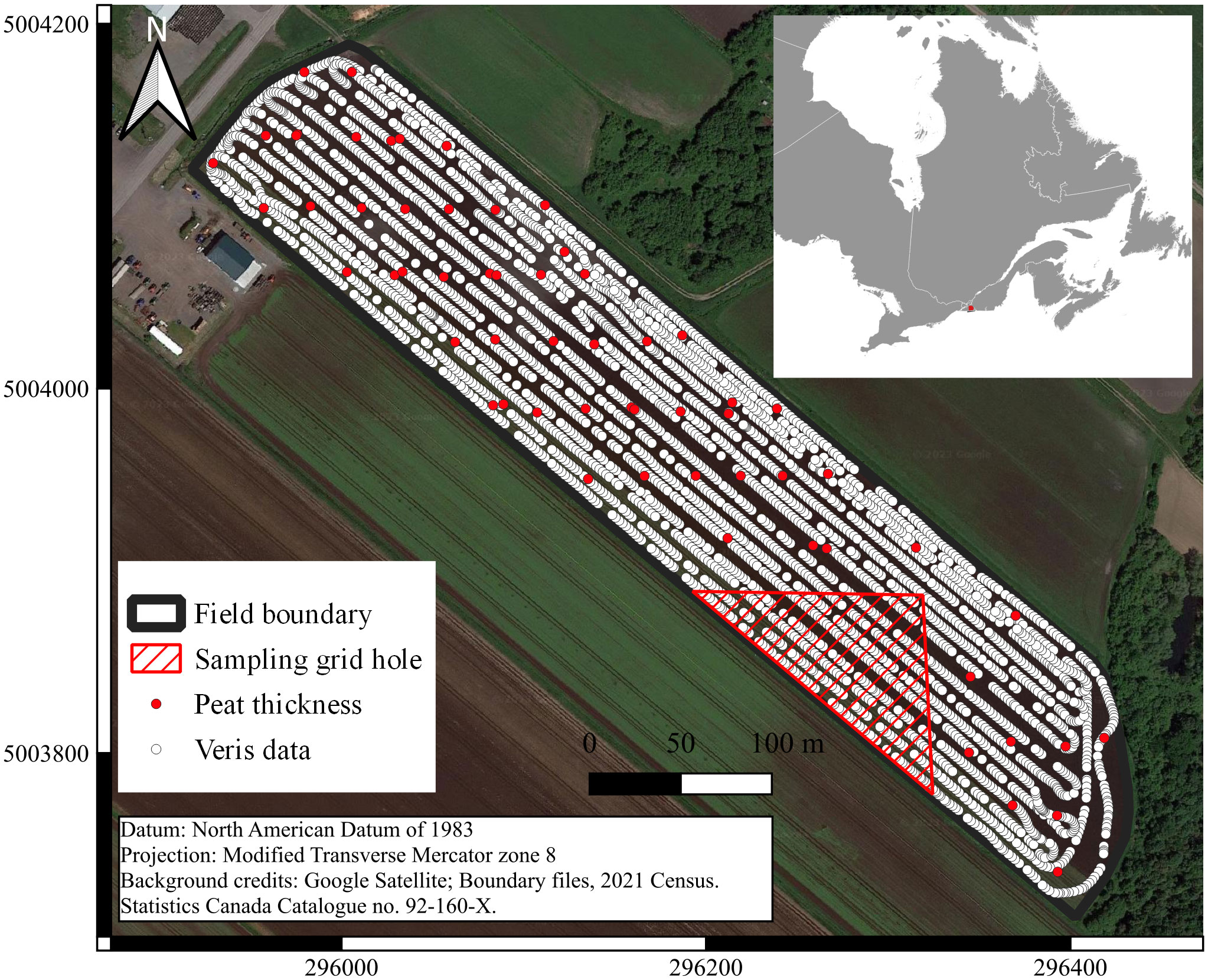
Figure 1 Study area showing the ground truth locations and the raw Veris data. A zone with no ground truth data can be seen on the southeast portion of the field.

2.2 Preprocessing of the environmental covariates

In this study, we used apparent electrical conductivity (ECa) measurement, digital elevation data, and a regional map of the MPT as predictors to train the models. Data preprocessing and modelling were carried out using the R statistical software (48). The descriptive statistics of the peat thickness and the environmental covariates are presented in Table 1, including the percentage of the coefficient of variation (CV), which measures the variability of a property. The CV was classified as follows: weak (<15%), moderate (15–35%), strong (35–50%), very strong (50–100%), or extremely strong (>100%) (49). The Pearson correlation coefficient (r) between the covariates was also computed.

TABLE 1

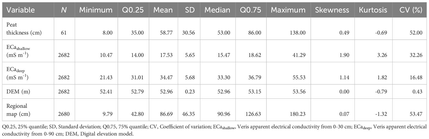
Table 1 Descriptive statistics of the predicted variable and the interpolated environmental covariates.

2.2.1 Veris apparent electrical conductivity

The ECa measurements were carried out in May 2021 using a Veris Q2800 (Veris Technologies, Inc., Salina, KS, USA; Figure 2) were collected in May 2021. It is a direct current resistivity sensor, compared to frequency-domain or time-domain electromagnetic instruments often used in peatland mapping studies (e.g., EM38, DUALEM-421S, ground penetrating radar, and time-domain reflectometer). Instead of emitting and detecting electromagnetic waves with a primary and secondary coil, the Q2800 consists of a series of coulters in contact with the soil surface acting as electrodes in a Wenner array configuration, generating a current arc that travels through the soil. The voltage decrease between the electrodes is then used to measure the resistance and infer soil ECa using Ohm’s law (50). Two current electrodes located in the center of the array complete the circuit with two inner potential electrodes (ECa_shallow) and two outer potential electrodes (ECa_deep). This intrusive electrical sensor has mostly been used in mineral soil studies. The Veris was tracked across the field at an average speed of 7 km h^-1 with a swath of 7 m between transects. This instrument measures the ECa, in mS m^-1, at two theoretical depth intervals simultaneously, equivalent to 90% of the response; 0-30 cm (ECa_shallow) and 0-90 cm (ECa_deep). Details regarding the calculation of the theoretical relative and cumulative instrument response to ECa with depth can be found in Sudduth et al. (50, 51). This relationship varies as a non-linear function of depth. The data was georeferenced with a Garmin 17x HVS receiver (Garmin International, Olathe, KS, USA). At the time of the survey, the field had a high water content and was even saturated at certain locations. Preliminary tests showed that the correlation between ECa_shallow and ECa_deep was lower and the data was less noisy when the soil was moister; therefore, Spring was chosen as an ideal data collection period.

FIGURE 2

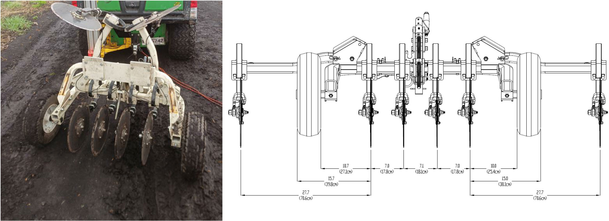
Figure 2 Image of the Veris Q2800 proximal sensor in transport mode (left) and schematic view of the configuration of the Veris Q2800 electrodes array (right). Image reproduced with permission, Veris Q2800 75 cm Row Spacing by Eric Lund, licensed under CC BY-SA, Veris Technologies.

The 3,548 ECa measurements were then preprocessed before the modelling steps. Duplicate values at the same coordinates were removed before filtering out the observations that fell outside of ± 3 standard deviations of the mean (52) since the instrument is prone to rapid drifts in the data (38). The coordinate system was transformed from geographic coordinates to planimetric coordinates (WGS84 to NAD93 MTM 8). The measurements were then interpolated using ordinary kriging (OK) with a block support. The experimental and theoretical variograms were computed using the gstat package (53, 54). Maps for ECa_shallow and ECa_deep at a 5-m spatial resolution were generated. The ECa_shallow required a log-transformation before modelling and was back-transformed following the method proposed by Laurent (55). The transformation was done to respect the normality assumption (low skewness and kurtosis) required by this interpolation method.

2.2.2 LiDAR digital elevation model

The region’s digital elevation model (DEM) was downloaded from the Données Québec repository. It was distributed by the Ministère des Forêts, de la Faune et des Parcs and derived from an aerial LiDAR survey. The DEM had a native spatial resolution of 1 m. The tile was clipped, aligned with the ECa interpolated maps, and resampled at a 5 m spatial resolution using a bilinear interpolation method. This step also removed part of the noise from the original data. Although the data was not acquired at the field-scale, this covariate was chosen because it was open-access, of high spatial resolution, and because it could be generated at the field-scale with a drone if needed (56).

2.2.3 Regional MPT map

A predictive map of the MPT generated at a regional-scale in a previous study (14) was at a 10 m spatial resolution but was resampled to a spatial resolution of 5 m using the nearest neighbour method and ensure its alignment with other covariates. The nearest neighbour approach was preferred over other resampling methods to avoid generating new interpolated values. This regional map (RM) was used as a baseline to compare the performance of the field-scale predictive models, but also as a covariate to assess the possibility of downscaling it. All models using the RM as a covariate were given the “-RM” suffix (e.g., Cubist-RM).

2.3 Modeling approaches

Two geostatistical models (OK and regression kriging), three machine learning algorithms (Cubist, Random Forest and Support Vector Regression) and a multiple linear model were tested for their ability to predict the MPT. All models, except OK, were fitted twice to the data: once with the DEM and ECa as predictors, and a second time also including the RM to evaluate the impact of its addition on the models, for a total of 11 models. The covariates described in the previous section were spatially intersected with the ground truth measurements to form a training dataset. The final predictions were made at a spatial resolution of 5 m and the final maps were created in QGIS (57).

2.3.1 Ordinary kriging

OK is an interpolation technique that provides the best linear unbiased predictions (i.e., aiming for no bias and minimized variance). To do so, a theoretical semivariogram model of the spatial autocorrelation between georeferenced observations is fitted to the experimental data. A prediction at unsampled locations can be made by using a weighted average of nearby observations, where the weights are a function of the modeled spatial autocorrelation and the distance to the predicted location (58). Here, multiple functions were tested along with isotropic and anisotropic semivariograms. This first approach to modelling the MPT was to generate an OK map with block support using ground truth observations. The map was generated the same way as for the ECa data. The residual sum of squares and the R² were used to find the best fit for the theoretical semivariogram. The range was recorded to provide a measure of the maximum distance at which two observations are spatially correlated. The purpose of the OK model was to evaluate, as a reference, the prediction performance of a manual sampling approach, without using any other covariate to predict the MPT.

2.3.2 Multiple linear regression

The multiple linear regression (MLR) aims to assess the relationship between multiple independent predictors and a dependent variable while minimizing the error associated with the fit (i.e., the residuals) (59). Compared to more complex models, it is intuitive to interpret and can tolerate a certain degree of correlation between the covariates. While this model is simple to compute, statistical assumptions must be verified. Two multiple linear regression (MLR and MLR-RM) models were fitted in two steps. A first stepwise model was fitted to the full set of covariates and non-significant ones were removed. For both models, ECa_deep was removed. Then, the statistical assumptions were validated (linearity, homoskedasticity and normality of the residuals, independence of errors and independence of the covariates). Finally, the model was applied to the set of interpolated covariates to generate a predictive MPT map for the field. In the final map, negative values were converted to zeros.

2.3.3 Multiple linear regression kriging

Regression kriging is a hybrid interpolation technique that combines deterministic and stochastic components to provide more accurate estimates of a variable (60). To improve the MLR models, a regression kriging workflow was implemented (MLRK and MLRK-RM). This was done under the assumption that the MLR models do not account for spatial autocorrelation. Because a spatial structure was expected in the residuals, it could be characterized and modelled with a semivariogram. Therefore, residuals from the MLR and MLR-RM models were extracted and interpolated with OK. The map of the residuals was added to the predicted MLR map. In the final map, negative values were converted to zeros. The sill and range for both theoretical semivariograms were recorded. The sill is a measure of the variability present in the dataset.

2.3.4 Cubist

This machine learner is a rule-based algorithm in the form of a model tree. Cubist decomposes the multivariate relationship between the dependent and independent variables at each node of the tree. Then, it fits linear models using one or multiple predictors, thereby minimizing the within-node variance. The terminal node of each branch consists of a linear model. The advantages of Cubist include its ability to capture both linear and nonlinear relationships in the dataset (61) and to avoid over and underfitting via the tuning of its two hyperparameters. Multiple trees can be aggregated with a boosting technique (i.e., the number of committees) and the final tree prediction is adjusted with a nearest neighbour search in the training data (i.e., the number of neighbours) (62, 63). The Cubist model was accessed through the caret package (64). Two models were trained: Cubist and Cubist-RM.

2.3.5 Random forest

Random Forest is a non-parametric decision-tree model based on ensemble modelling theory (65). It makes use of a bootstrapping approach to sample with replacement the original dataset and generates multiple prediction trees. The trees are then aggregated to obtain an average prediction that is less biased than a single-model tree (62). Its hyperparameters are m_try, the number of randomly selected predictors used at each node of the tree to divide the dataset by minimizing the within-node heterogeneity, and N_Trees, the number of trees to be computed and aggregated, which was set to the default value of 500. RF and RF-RM were trained using the caret package in R.

2.3.6 Support vector regression

Support Vector Regression (SVR) is a generalization of the support vector machine algorithm used for classification purposes. Instead of maximizing the decision boundaries between two classes by finding the best support vectors to minimize the classification error, SVR fits a regression hyperplane to the training sample in a higher dimensional space. An ε-insensitive region, or ε-tube, is optimized around the regression hyperplane so that most training observations are contained by it. The advantage of SVR is its ability to transform non-linearly separable data to linearly separable data in a higher dimension by projecting it using a kernel function. After testing multiple kernels, a radial basis function kernel was selected using the caret and kernlab packages (66, 67). Then, the model was trained to find the best cost (C) and sigma hyperparameters specific to the radial kernel. C controls the penalty associated with observations that fall outside the ε-tube. For instance, a high C leads to higher penalties and larger margins (i.e., the width of the ε-tube within which observation departures from the regression hyperplane will not penalize the model during the optimization phase), leading to a lower prediction bias and larger variance. Sigma controls the linearity of the margins by adjusting the weight of the individual training observations. SVM and SVM-RM were trained this way. More information about the theory behind SVR can be found in other references (68).

2.4 Performance metrics

Two accuracy metrics, three error metrics, and the range of the predicted values were extracted for every model, and used to tune the hyperparameters. The coefficient of determination (R²) and Lin’s concordance correlation coefficient (CCC; eq. 1) were used as accuracy metrics to evaluate the relationship between the observed and predicted variables and their departure from the 1:1 line (69). Compared to the R², CCC corrects the agreement between two variables in the presence of a systematic bias:

$\begin{array}{ll}CCC= \frac{2s_{op}}{{(\overline{o}-\overline{p})}^2+ s_o^2+ s_p^2}& (1)\end{array}$

where s_op is the covariance between predicted and observed values, the s² are their corresponding variance, $\overline{o}$ is the mean of the observed values, and $\overline{p}$ is the mean of the predicted values.

The root mean square of error (RMSE, eq. 2), mean absolute bias (MAB, eq. 3), and mean bias error (MBE, eq. 4) complemented the accuracy metrics by representing the precision of the predictions. The equation for RMSE is:

$\begin{array}{ll}RMSE= \sqrt{{\sum }_{i=1}^N\frac{{(O_i-P_i)}^2}{N}}& (2)\end{array}$

where O is the observed value and P the corresponding predicted value for the i^th observation, and N is the total number of observations. The MAB and MBE were calculated as follows:

$\begin{array}{ll}MAB= {\sum }_{i=1}^N\frac{|O_i-P_i|}{N}& (3)\end{array}$

$\begin{array}{ll}MBE= {\sum }_{i=1}^N\frac{O_i-P_i}{N}& (4)\end{array}$

The MBE reports the average difference between the observed and predicted values; the MAB reports the average, absolute difference between observed and predicted values; and the RMSE reports the spread of the individual errors. Similar values of RMSE and MAB indicate similar errors across the predicted range, while the MBE indicates a tendency to underestimate (negative value) or overestimate (positive value).

2.5 Model tuning

A leave-one-out cross-validation (LOOCV) procedure was selected to evaluate all models for its simplicity and due to the lack of an external data set for validation. Nonetheless, some models required adjustments to this procedure to be carried out. For the OK model, the performance metrics were calculated using the predicted values from the LOOCV procedure with a local neighbourhood of 16 observations implemented with the krige.cv function. For the machine learners, the hyperparameters were tuned using an LOOCV procedure and the CCC as the metric to select the best tuning parameter. The same LOOCV predictions were used to compute the model performance metrics. Then, a final model was trained using that set of hyperparameters and used to make a prediction for the entire field.

For the MLR models, the observed and predicted values were used to compute the performance metrics. Regarding the MLRK models, a LOOCV loop was implemented as follows. First, the MLR model was computed, along with a semivariogram of the residuals of all 61 observations. Then, one observation was removed. The MLR model was computed again and applied over the field. A residual map was produced and added to the MLR prediction map. Finally, the out-of-the-bag observation was spatially intersected with the final map to compare the predicted and observed values. This procedure was repeated for every observation to calculate the performance metrics. Here, it is important to note that the R² and CCC metrics are pseudo-statistics since there were no repeats in the LOOCV procedure. It was therefore impossible to compute these statistics on every fold (i.e., on one observation). The out-of-the-bag predictions were aggregated to form a dataset on which these two metrics were calculated. Since it was impossible to carry out the LOOCV procedure for the RM, the 61 observations were spatially intersected with it and the performance metrics were calculated by comparing the observed and the predicted values. The performance metrics and ranges from the semivariograms of the depth to the mineral layer and of the limnic layer thickness were also extracted for the RM from Deragon et al. (14).

2.6 Prediction uncertainty

To compare the uncertainty of the predicted maps more fairly between the geostatistical and machine-learning models, a quantile regression post-processing approach (QR) was used for all models. This method was generalized and adapted to digital soil mapping by Kasraei et al. (70) and was recently compared to other ways of validating prediction uncertainty with good results (71). QR can compute a linear regression model for any quantile of a given dependent variable’s conditional distribution, compared to a standard linear regression which computes the mean of the dependent variable. The underlying assumption is that the observed and predicted values follow a linear relationship. First, a QR model was fitted to obtain the conditional quantile function of the predicted values from the models (e.g.: Cubist, OK, MLRK, etc.) conditioned by the observed values. This procedure was repeated twice, to compute the 5^th and 95^th quantiles regressions. This was done using the qr function from the package quantreg (72). Then, maps for the lower and upper limits were generated by combining the predicted map for the field and the QR models. Finally, the 90% confidence interval was generated by subtracting the 95^th and 5^th quantile maps. The QR uncertainty model is separated from the actual predictive model, making it a model-agnostic procedure (71).

3 Results

3.1 Descriptive statistics and maps of the covariates

The MPT recorded from the ground truth measurements ranged from 8 to 138 cm, while the regional map predicted values between 9 and 180 cm (Table 1, Figure 3A). A 1 m difference in elevation was observed between the lowest and highest points of the field, with a uniform gradient from the northwest to the southeast (Figure 3B). The predicted MPT from the RM showed a similar spatial pattern to that of the DEM, which was further evidenced by the high Pearson correlation coefficient between them (r = 0.76). Regarding the CV of the covariates, a very strong variability was associated with the MPT (52.0%) and the RM (53.5%). The CV was lowest for the DEM (0.4%), but it was expected since absolute elevation was used. The ECa_deep (CV = 16.5%) showed variability on the low end of moderate, compared to the ECa_shallow variability (CV = 32.3%), which can be observed in Figures 3C, D. Overall, the CV indicated the presence of spatial heterogeneity across the field.

FIGURE 3

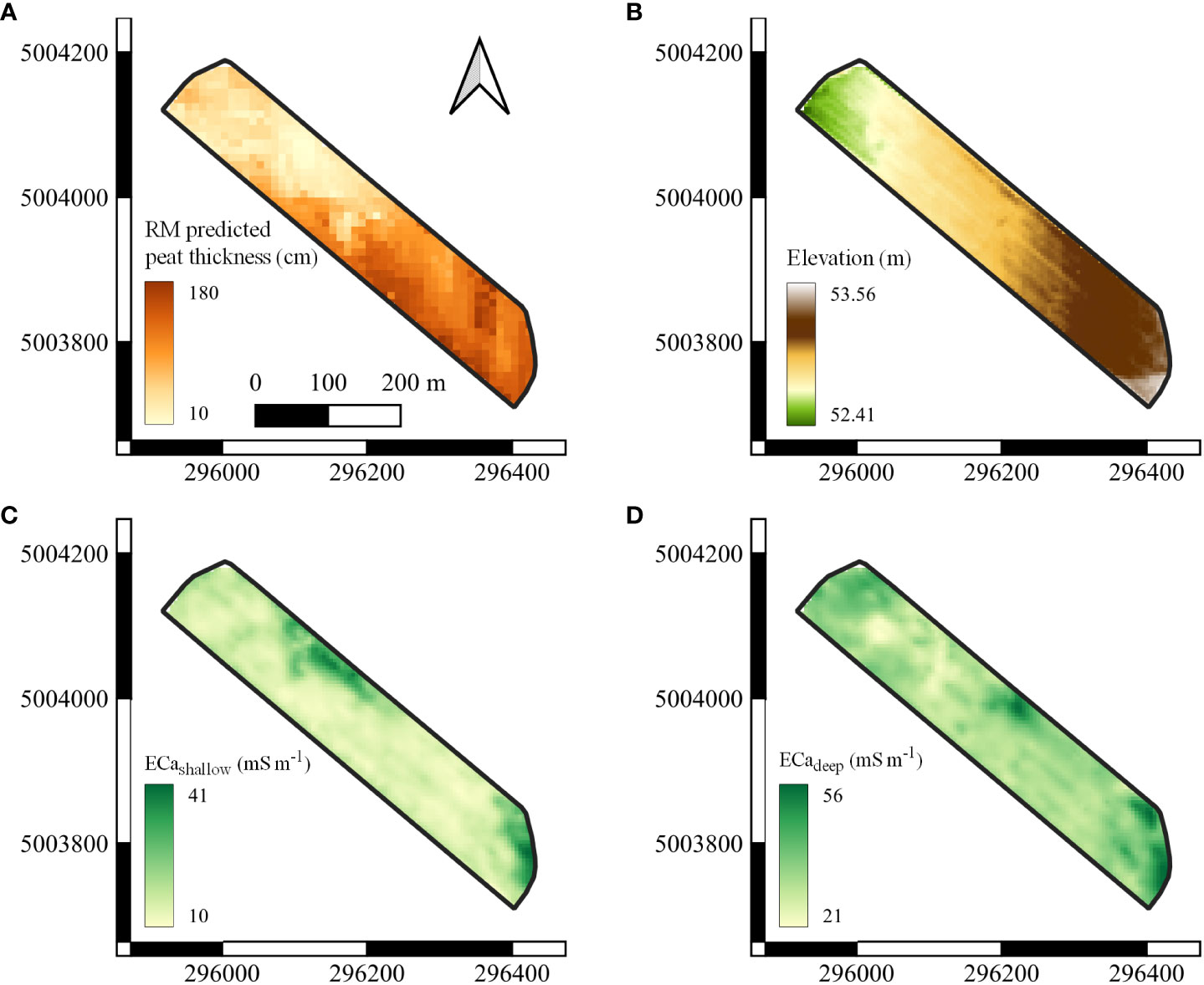
Figure 3 Maps of the covariates. (A) The predicted maximum peat thickness from a regional map by Deragon et al. (14), (B) the digital elevation model, (C) the shallow measurements of the apparent electrical conductivity (ECa_shallow), and (D) the deep measurements of the apparent electrical conductivity (ECa_deep) by the Veris Q2800.

3.2 Fitting the semivariograms for the geostatistical approaches

The best fit for the semivariogram of the MPT for the OK approach was achieved with a Gaussian model. Here, an effective range of 57 m was observed. For the MLRK model fitted on the residuals, a sill of 617 cm² and an effective range of 34 m were obtained with an exponential model (Figure 4). The residuals of the MLRK-RM model had a lower sill (298 cm²). The best fit was also achieved with an exponential model and had an effective range of 29 m. These ranges were smaller than the ones for the mineral layer (957 m) and of the limnic layer thickness (4,733 m) obtained at the regional scale (14).

FIGURE 4

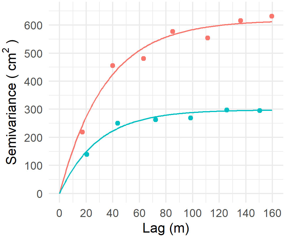
Figure 4 Experimental (points) and theoretical (lines) semivariograms of the residuals of the multiple linear regression model (MLR, in red) and the multiple linear regression model with the regional map (MLR-RM, in blue). A semivariogram plot illustrates the change in autocorrelation (or variance) between two observations spaced by an incremental distance called lag.

3.3 Model performance

By intersecting the ground truth observations with the RM, a CCC = 0.65 and RMSE = 30 cm was obtained (Table 2, Figure 5A). When compared to the overall RM for the whole region, the model performance was slightly better for this field. Nonetheless, this map had the highest error and lowest accuracy compared to all the other models from this study. Its MBE was also the highest, indicating a strong tendency to overestimate the MPT. The MBE was close to zero for all other models, with a tendency towards overestimation for the MLRK models and underestimation for the machine learners.

TABLE 2

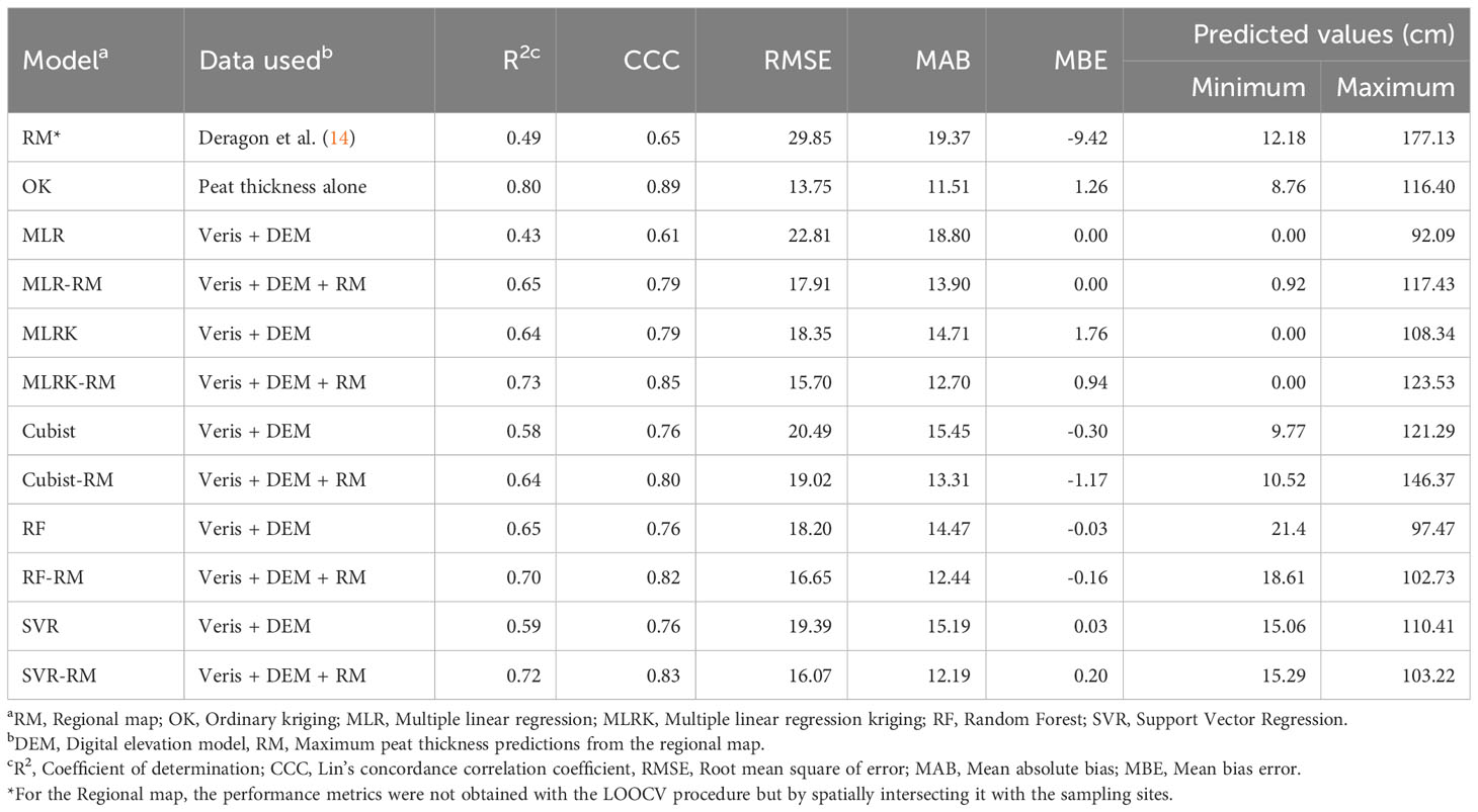
Table 2 Model performance metrics following the leave-one-out cross-validation (LOOCV) procedure for each model.

FIGURE 5

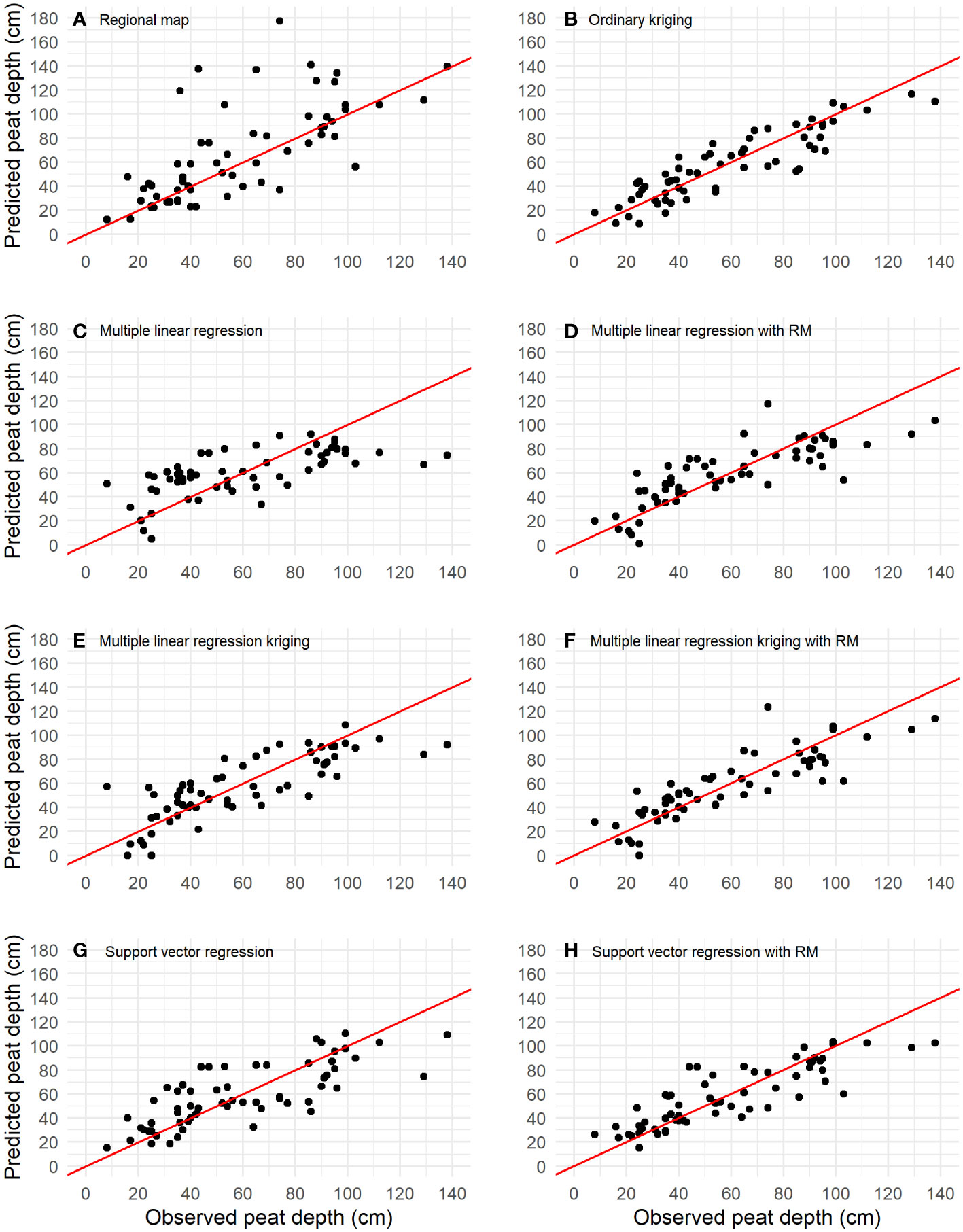
Figure 5 Scatterplots of the relationship between the observed and predicted values for a selection of the final models: (A) Regional map, (B) Ordinary kriging, (C) Multiple linear regression, (D) Multiple linear regression with RM, (E) Multiple linear regression kriging, (F) Multiple linear regression kriging with RM, (G) Support vector regression, and (H) Support vector regression with RM. The red line represents a perfect 1:1 relationship between observed and predicted observations.

The LOOCV procedure resulted in the lowest error (RMSE = 14 cm) and highest accuracy (CCC = 0.89) metrics for the OK model (Table 2). The good fit of the theoretical semivariogram and the LOOCV results of the OK model confirmed that a strong spatial structure existed for the MPT. The second-best model was the MLRK-RM (RMSE = 16 cm, CCC = 0.85). This model did not significantly improve on the OK model. The best machine learner was SVR-RM, showing an RMSE = 16 cm and CCC = 0.83. The geostatistical approaches performed slightly better than the machine learners. Despite their better performance metrics, the Cubist-RM model had the closest predicted range to the ground truth data (11-146 cm). The other models tended to underpredict the deeper deposits in the field, especially the observations with an MPT > 100 cm, as can be seen in Figure 5.

The machine learners and the MLRK approach resulted in an increase in CCC and a decrease in RMSE when the RM was added as a predictor. The average increase in CCC and decrease in RMSE associated with the addition of the RM as a covariate were 0.08 and 2.8 cm, respectively (Table 2). The Veris data combined with the DEM always led to more accurate estimates than the RM alone. ECa_shallow was an important predictor in the models; however, ECa_deep had a low predictive power in all machine learning models. The Pearson correlation coefficient between ECa_shallow and ECa_deep was r = 0.002 in the training data and r = 0.35 across the field’s extent, indicating a low correlation between them.

3.4 Predicted maps and uncertainty estimates

The predicted maps for six of the models are presented in Figure 6. All maps showed similar spatial patterns to the RM, except in the southeast portion of the field where the latter overestimated the MPT. In addition, artifacts related to the incorporation of the RM in specific models were observed (Figures 6D, F). Other fine-scale artifacts were observed for the SVR model (Figure 6E) due to the ECa data, whereas the MLRK map (Figure 6C), which used the same covariates, had a smoother appearance. The missing portion of the sampling grid influenced the OK map, where a triangular shallow zone was wrongly extrapolated (see Figure 1) and hence, the resulting map should not be used for that extrapolated area. By comparing the predicted maps to those of the environmental covariates (Figure 3), the shallowest zones corresponded with where the Veris ECa values were highest.

FIGURE 6

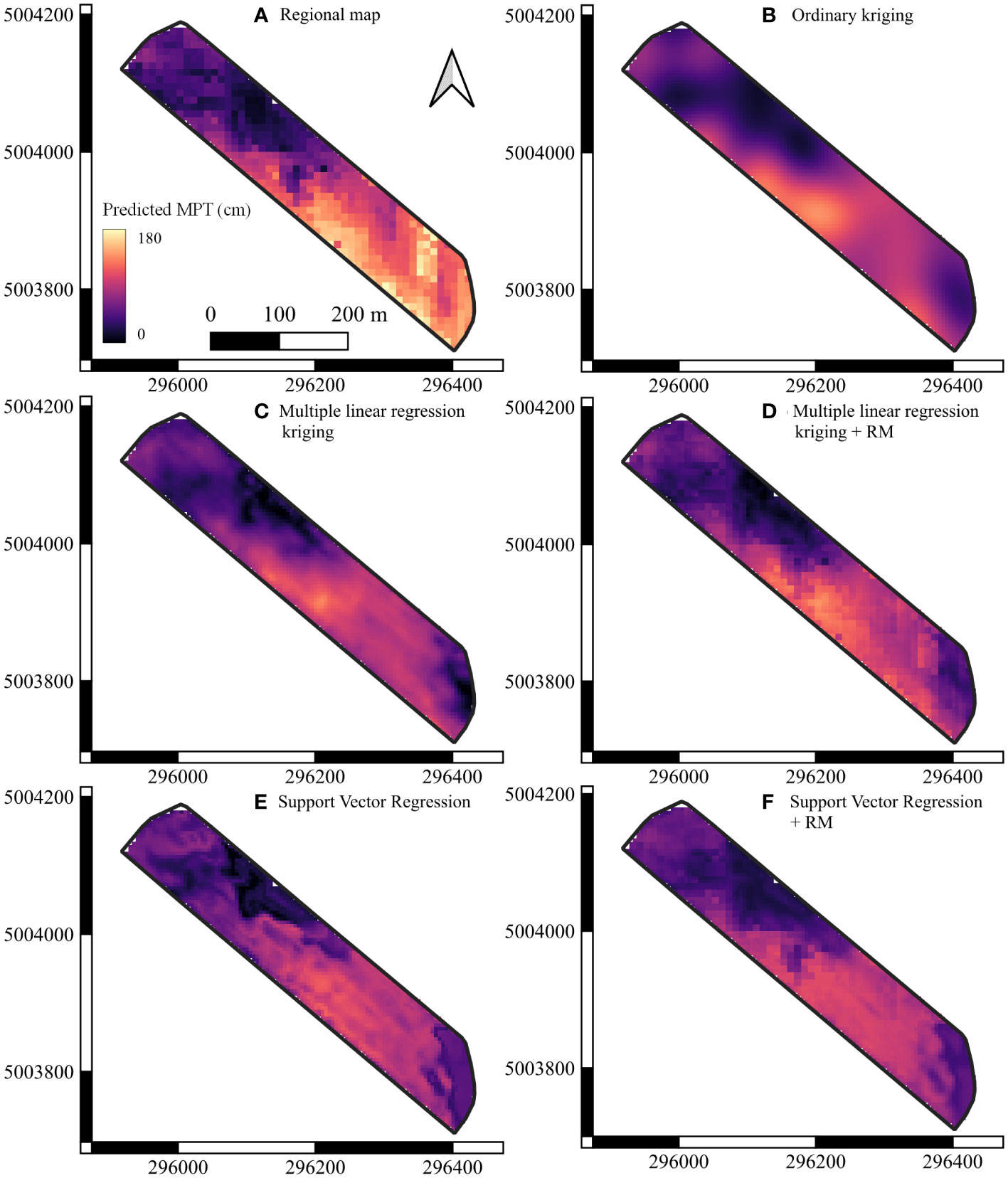
Figure 6 Maps of the predicted maximum peat thickness (MPT, cm) for six of the models: (A) Regional map, (B) Ordinary kriging, (C) Multiple linear regression kriging, (D) Multiple linear regression kriging with the regional map, (E) Support Vector Regression, and (F) Support Vector Regression with the regional map. All maps have a spatial resolution of 5 m and share the same legend.

The uncertainty maps of the three best models, OK, MLRK-RM and SVR-RM, are presented in Figure 7. The 90% confidence interval range of values for the OK model (32 to 69 cm) was lower than that of the MLRK-RM model (24 to 80 cm) and the SVR-RM model (35 to 82 cm), indicating an overall smaller prediction uncertainty. Furthermore, the difference between the widest and narrowest prediction interval within each prediction uncertainty map was the smallest for the OK map. This indicates fewer differences in prediction uncertainty across the field than the other two best models. Moreover, the spatial distribution of the uncertainty showed similar patterns to the predicted map (i.e., higher uncertainty was associated with higher predicted values).

FIGURE 7

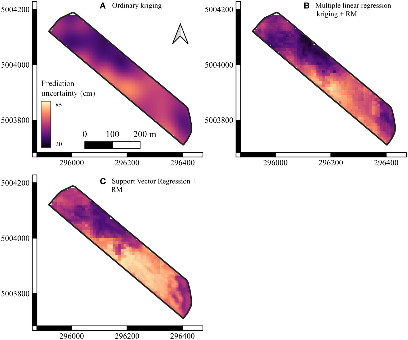
Figure 7 Prediction uncertainty (cm) maps of the three best models: 90% confidence interval map for the (A) Ordinary kriging, (B) Multiple linear regression kriging with the regional map, and (C) Support Vector Regression with the regional map models. All maps have a spatial resolution of 5 m and share the same legend.

4 Discussion

4.1 Interpreting model performance

Based on the results, direct, field-scale mapping of the MPT was possible with high accuracy. This allowed the production of more precise maps than the RM by avoiding the propagation of errors linked to the determination of the depth to the mineral layer and limnic layer thickness individually. The superiority of the OK model indicated the presence of a strong spatial structure at the field-scale in the dataset. The range of 57 m obtained with the Gaussian theoretical model supports this claim. Furthermore, compared to the 4,733 m range for the limnic layer thickness and the 957 m range for the depth to the mineral layer at the regional scale (14), a field-scale approach to study and predict the MPT seems more appropriate. It was also possible to downscale the RM by using it as a covariate, making use of previous mapping efforts. For instance, adding the RM as a predictor in the MLRK-RM model reduced the sill (i.e., variance) of the residuals twofold compared to MLRK (Figure 4). This indicated lower prediction error from the MLR model, which was supported by better performance metrics (Table 2). The RM was trained using only remote sensing covariates and was generalized to a greater extent than only this field, leading to the worst fit compared to the other models when used alone to predict the MPT. Nonetheless, the fact that the RM map captured spatial patterns outside and around the field added new information to the model. The RM acted as a general trend of the MPT for the field based on the surroundings. This could explain the observed increase in model performance when this predictor was added to the models. Supplementing the RM with proximally sensed data also improved the MPT predictions in the southeast portion of the field (Figure 6). All models captured the shallow values where the RM predicted higher values erroneously.

There was not a major difference in model performance or prediction uncertainty between the three best models (i.e., OK, MLRK-RM, and SVR-RM, Figure 7). Assuming a fair comparison between the models, SVR-RM could be a potential candidate for future studies. While OK required fewer steps to generate the map and MLRK-RM allowed for a better understanding of the predictors via the deterministic portion of the model, they both required the computation of a theoretical semivariogram to fit the observed data. If a minimum number of observations is not available, the model performance will suffer (58), which can be especially problematic for smaller fields. Furthermore, statistical assumptions must be met for both models and can limit the applicability of the method in certain situations. On the other hand, SVR-RM could work on smaller datasets, decreasing the manual labour required for modelling the MPT. It is worth noting that the OK model, the only one not using the covariates, had better performances than SVR-RM and MLRK-RM (Table 2). Two potential reasons could explain this better performance. First, pairs of observations were close to each other at seven locations in the sampling grid and had different observed MPT values. Nonetheless, they had similar or the same covariate values as they fell in the same grid cell. This might have led to a poor understanding of the relationship between the MPT and the covariates in the MLR and SVR models. This small-scale variation in soil stratigraphy is similar to the nugget effect—essentially a part of the variance that will never be explained. Second, the selection of covariates was limited in this study and their relationship with the MPT may have been affected by other factors (see section 4.2.2). While it is not possible to compare these results to other MPT studies, we can compare them to standard peat thickness studies at the field-scale using similar covariates. For instance, Koszinski et al. (47) modeled the peat thickness with an EM38DD and airborne LiDAR data in 7 nearby agricultural fields. For an observed range of 0-190 cm of peat thickness, they observed an R^2 = 0.61 with their model. Beucher et al. (33) measured the ECa with a DUALEM-421S and used a LiDAR DEM along with terrain attributes. Their best model, an MLR, had high accuracy (CCC = 0.94) and low error (RMSE = 65 cm) for a range of observed peat thickness between 3 and 730 cm. Koganti et al. (43) returned in the same field as the previous study using a portable gamma-ray sensor and terrain attributes to map the peat thickness. Their best model, ordinary kriging, achieved a CCC= 0.97 and an RMSE = 0.59 m, which was very similar to the performance of their second-best model, empirical Bayesian kriging regression (CCC= 0.97 and an RMSE = 0.63 m). The latter included covariates. These accuracy metrics from previous studies are in the same range of performance as ours and the error, if standardized with the range of observed values, are comparable to the ones we observed.

4.2 Limitations of the study

4.2.1 The MPT dataset

Given the small to moderate number of ground truth measurements, the LOOCV procedure was chosen to evaluate our models and more easily compare them with the RM. Yet, it may have overestimated the model accuracies by not accounting for spatial autocorrelation (73). Resampled measures were not possible in this study. With a larger dataset, a k-fold cross-validation procedure or an additional validation dataset could have been used to form training, testing and validation partitions to tune and evaluate the performance of the machine learners. For instance, Deragon et al. (14) trained their models on spatial and standard LOOCV and obtained substantially better results with standard LOOCV. The sampling design was oriented towards a geostatistical approach with a uniform sampling grid. It may have led to a biased performance evaluation for the machine learners since they require good feature space coverage. For these reasons, the machine learners were tested to provide a comparison to the geostatistical approaches but could perform better if the sampling design were to be adapted. The effect of the sampling density on the model performance should also be evaluated in a future study by removing observations from the dataset iteratively (43). A sampling density of around 10 samples per hectare is on the high end compared to other studies and might not be realistic for smaller fields and practical applications of the method. Moreover, the range of values of MPT > 100 cm was represented by only 4 observations in our dataset (Figure 5). The unbalanced coverage of the MPT range by the sampling design could partially explain why the model fit was lower for higher predicted values of MPT. In other words, future studies should seek to improve the methodology and replicate it for multiple fields as a case study to assess how our results could apply to other fields.

4.2.2 Drivers of the electrical properties of soil layers and related errors

The electrical properties of peat are mostly driven by the water content and the concentration of dissolved ions, which are related to the porosity and bulk density. These factors determine the resistivity, or conductivity, of the material. Peat has a higher porosity compared to mineral layers, and therefore a generally higher water content and apparent dielectric permittivity (Ka) (74). In the past, differences in pore water conductivity were observed between peat and the underlying mineral layer (32, 33). The peat decomposition level, CEC, and temperature can also affect ECa readings (32, 75). Regarding the properties of limnic layers, Lange et al. (76) found a decrease in bulk density and an increase in total porosity and salinity of limnic layers compared to the overlying peaty layers. This is coherent with properties reported in other studies (2, 21, 22). In general, it can be said that peaty layers are more resistive than mineral and limnic layers, especially at lower water contents (27, 47, 74).

Therefore, variations in these properties can affect the vertical resolution of the Veris ECa and impact MPT predictions (50). Anthropogenic activities can affect water regimes and salt movement in the soil profile via capillary rise (77). Moreover, agriculture often leads to the formation of a compacted layer near the surface (78, 79) and requires fertilizer inputs that will impact surface soil salinity (46). Drain tiles can also introduce artifacts in readings of certain sensors, potentially adding random noise to the ECa signal since we can expect variations in these factors across the field. We can also expect ECa_deep to be more sensitive than ECa_shallow given its greater vertical sensing range. This could partially explain why ECa_deep had a low predictive power and the models underpredicted the observations with an MPT > 100 cm. Variations in the electrical properties of the soil layers could have impacted the sensing depth of the Veris Q2800. Moreover, compared to other EMI instruments, the Veris Q2800 has only two simultaneous exploration depths. Some EMI instruments can have 4 or even 6 depths of conductivity sounding with a greater depth of exploration. This sensitivity to deeper layers can lead to a higher vertical resolution.

4.3 Implications on soil conservation practices

The initial goal in generating MPT maps was to support precision soil conservation practices at the field-scale (13). Three management zones have been suggested: MPT< 60 cm, 60-100 cm, and > 100 cm. Such zones were needed to determine where biomass amendments would be added in priority to compensate for mineralization losses and avoid changes in physical and chemical properties (7, 13). The RMSEs of the best models at field-scale are twice as low as the one of the RM, resulting in a more accurate classification of MPT zones in a field. Furthermore, the Montérégie region possesses an RM that serves as a first rough estimation of the MPT for farms where soil measurements were taken and for others that do not have soil databases. Even if the RM was not accurate enough, it is better than no estimation at all. Farmers could greatly improve the accuracy of the MPT predictions at field-scale by combining the map with proximal sensor data. A reduction of manual sampling points can be expected, although a small number will always be required to validate predictions. This improvement can be related to the fact that proximal sensors can generate a high density of observations to better capture the fine-scale variations in the peat thickness. Veris data does not require calibration and the equipment can easily be tracked by an ATV, which is an advantage for the end-user of this methodology: farmers or agronomic consultants. For now, a field-by-field approach would be more advisable since the applicability and generalization of the SVR-RM model to other fields are unknown. Extrapolation of OK and MLRK-RM models to other fields is simply impossible due to the nature of geostatistic models.

To limit sources of uncertainty related to ECa measurements caused by the surveying season, we opted for a Spring survey. We recommend Spring or Fall to monitor ECa to evaluate the MPT. Peat near the soil surface tends to become hydrophobic when it dries with evapotranspiration, tillage, and drainage (80, 81), which may occur during the Summer. In our preliminary tests, we observed poor contact between the electrode coulters and the soil, which is more granular than deeper, untilled peat material. A poor contact resulted in noisier data and potentially a shallower depth of exploration for ECa_deep. This led to a smaller range of ECa measurements compared to the Spring period, and a higher correlation between ECa_shallow and ECa_deep. A significant water content gradient between the dry surface layer and the underlying layers beneath the compact layer, generally found around 30 cm, can introduce bias in the measurements. This depth coincides with the peak sensitivity of the Veris Q2800. With a more homogeneous water content in the soil profile, the sensing depths of both measured ECa should be more distinct. Therefore, the correlation between the measured values should decrease. During summer, the temperature profile can also vary significantly (around 30°C on the soil surface and around 8-10°C at a depth of 90 cm). However, during Spring and Fall, the temperature is more constant throughout the soil profile. For practical reasons, we also recommend these periods as it is easier to access an empty field without a snow cover or crops. Two caveats are associated with measurements in soil with a higher water content; the salinity level of peat is expected to be closer to that of limnic layers (2), and the soil must provide enough bearing capacity to support the weight of the equipment.

The extent of limnic soils worldwide is unknown, but estimations are available for certain countries; Canada: 32,057 ha and Sweden: 48,915 ha (14, 20). Many other countries have reported the presence of this layer, even though the extent might not have been reported in the form of a map for the country. As stated by Berglund and Berglund (20), limnic layers are uncovered with soil loss and subsidence, leading to increased risks for cultures. Since this phenomenon is not unique to Canada, the proposed field-scale approach could be relevant to other countries needing crucial soil data to support soil conservation interventions.

4.4 Mapping the MPT in future work

Although this study showed that direct mapping of the MPT was possible for shallow soils, other surveys should evaluate the methodology for thicker deposits. The methodology could be improved to map the three materials individually to also acquire spatial information about the depth and thickness of the limnic layer at the field-scale. A better vertical resolution could be obtained by first quantifying discriminant physical and chemical properties of peaty, limnic and mineral layers. This would support the selection of more appropriate proximal sensors or automated probes (22). Moreover, an approach based on multi-sensor fusion (44) could be used to take advantage of multiple technologies at once. Using sensors with a greater sensing depth could solve the underestimation issue for the site with an MPT > 100 cm observed in this study. EMI and gamma-ray spectrometers are examples of proximal sensors to test (33, 43). In optimal conditions, we should be able to map and distinguish the three materials (mineral, limnic and peaty layers) at greater depths to better inform farmers and to generate maps of the C stocks simultaneously. Proximal sensors should also be chosen for their sensitivity and specificity to a target property to limit the influence of other factors. We do not believe that ground penetrating radar or electrical resistivity tomography were appropriate technologies in this agricultural context, despite their effectiveness at detecting limnic layers in past studies (27, 30, 82, 83). For instance, Sass et al. (27) were able to detect limnic layers in alpine mires using a ground penetrating radar and electrical resistivity tomography. However, they concluded that manual probing was still needed to validate the result. Other limitations of these technologies include the need for site-specific calibrations, the data output that is less compatible with the digital soil mapping workflow and the fact that they cannot be used as on-the-go sensors. Nonetheless, these studies also provided measurements of electrical conductivity and permittivity for peat and limnic layers.

To increase the vertical resolution of the predicted MPT, other geophysical techniques could be used, such as the inversion of the ECa data. Since the depth-weighted response function of the signal is known for ECa instruments, the ECa can be converted to the true apparent electrical conductivity (ECr) for every point of a soil profile using an inversion software. In short, the apparent bulk electrical conductivity is the sum of infinite layers of soil with an ECr (e.g., ECa 0-30 cm = ECr 0-10 cm + ECr 10-20 cm + ECr 20-30 cm). It is an alternative that allows the production of quasi-2D or quasi-3D maps of soil electrical conductivity, which are correlated with soil type variations and stratigraphy via sharp or smooth gradients. In the peatland mapping literature, it is possible to find multiple examples of ECa inversion to predict peat thickness (e.g., 33, 35, 36). While the inversion often leads to a better understanding of the stratigraphy and the petrophysical properties of the materials, raw ECa measurements combined with other modelling techniques can sometimes lead to more accurate predictions of the peat thickness (33, 35). Data inversion is also often done using EMI equipment with four or six depths of exploration, rarely two like the Veris Q2800; the more signals overlap, the better the inversion.

It is unknown how important the DEM would be in predicting the MPT in areas with a greater difference in elevation than the one observed in this study. We expected the DEM to be less relevant in areas with highly variable stratigraphy not captured by the DEM. We also expected the limnic layer, a sedimentary material, to have deposited mostly in relatively flat zones. This can affect the relationship between the DEM and the MPT. Nonetheless, a DEM and its derivatives were used in studies at different scales (14, 33, 43, 84) generally contributing to the predictive power of the models. One advantage of the addition of the DEM is that it could capture soil water content differences across a field with varying elevation. These differences can affect the readings of proximal sensors. Moreover, topographical and hydrological covariates can be derived from the DEM as other potential covariates (e.g., slope, aspect, wetness index).

5 Conclusion

We evaluated the potential of mapping at field-scale the maximum peat thickness—a measure of the cultivable peat layer until either the mineral layer or a limnic layer is encountered, using soil ECa from a direct current resistivity sensor and elevation in a shallow cultivated organic soil, in addition to a regional map of the MPT. Our results suggest that it is possible to predict the MPT with various modelling techniques; however, geostatistical approaches performed better. Results showed that the ECa and the elevation could capture the transition between the peat-limnic and peat-mineral layers, significantly improving the accuracy of the regional map for the same area. The addition of the regional map as a covariate also improved all models, allowing them to downscale the former. This study suggests a useful field-scale approach to form soil conservation management zones for farmers and agronomic consultants with much less sampling efforts than manual sampling alone.

Data availability statement

The datasets presented in this article are not readily available because of the nature of this research. This data is of strategic importance for the research partners and is considered sensitive information. Requests to access the datasets should be directed to Raphaël Deragon, raphael.deragon.1@ulaval.ca.

Author contributions

RD: Conceptualization, Funding acquisition, Investigation, Methodology, Writing – original draft, Writing – review & editing. BH: Methodology, Supervision, Writing – original draft, Writing – review & editing. NL: Conceptualization, Investigation, Supervision, Writing – review & editing. KJ: Methodology, Writing – review & editing. AC: Methodology, Writing – review & editing. JC: Conceptualization, Funding acquisition, Resources, Supervision, Writing – review & editing.

Funding

The authors declare that this study received funding from a Postgraduate Scholarship – Doctoral (PGS D) by the Natural Sciences and Engineering Research Council of Canada (NSERC) and a Doctoral scholarship (B2X) by the Fonds de recherche du Québec-Nature et technologies (FRQNT) granted to R. Deragon. The authors also acknowledge the financial support of the NSERC through an Industrial Research Chair Grant in Conservation and Restoration of Cultivated Organic Soils (IRCPJ 411630–17) in partnership with Delfland Inc., Le Potager Riendeau Inc., Productions maraîchères Breizh inc., Les Fermes R.R. et fils inc., La Production Barry inc., Maraichers J.P.L. Guerin & fils, Le Potager Montréalais ltée, R. Pinsonneault et fils ltée, Patate Isabelle Inc., Fermes Hotte et Van Winden Inc., Les Fermes du Soleil Inc., Les Jardins A. Guérin et Fils Inc., Vert Nature Inc., and Production Horticole Van Winden. The funders were not involved in the study design, collection, analysis, interpretation of data, the writing of this article or the decision to submit it for publication.

Acknowledgments

The authors would like to thank Dr. Lotfi Khiari for his early contribution to the project with his insights on the kriging models. We are also grateful for the constructive and insightful comments received from the reviewers.

Conflict of interest

The authors declare that the research was conducted in the absence of any commercial or financial relationships that could be construed as a potential conflict of interest.

Publisher’s note

All claims expressed in this article are solely those of the authors and do not necessarily represent those of their affiliated organizations, or those of the publisher, the editors and the reviewers. Any product that may be evaluated in this article, or claim that may be made by its manufacturer, is not guaranteed or endorsed by the publisher.

References

1. Minasny B, Berglund Ö, Connolly J, Hedley C, de Vries F, Gimona A, et al. Digital mapping of peatlands - A critical review. Earth Sci Rev (2019) 196. doi: 10.1016/j.earscirev.2019.05.014

CrossRef Full Text | Google Scholar

2. Minasny B, Adetsu DV, Aitkenhead M, Artz RRE, Baggaley N, Barthelmes A, et al. Mapping and monitoring peatland conditions from global to field scale. Biogeochemistry (2023). doi: 10.1007/s10533-023-01084-1

CrossRef Full Text | Google Scholar

3. Kroetsch DJ, Geng X, Chang SX, Saurette DD. Organic soils of Canada: part 1. Wetland organic soils. Can J Soil Sci (2011) 91(5):807–22. doi: 10.1139/CJSS10043

CrossRef Full Text | Google Scholar

4. Parent L-É, Ilnicki P. Organic soils and peat materials for sustainable agriculture. Boca Raton, Florida: CRC Press (2003).

Google Scholar

5. Vepraskas MJ, Craft CB. Wetland Soils : Genesis, Hydrology, Landscapes, and Classification. Boca Raton, Florida: CRC Press (2016).

Google Scholar

6. Bourdon K, Fortin J, Dessureault-Rompré J, Caron J. Agricultural peatlands conservation: How does the addition of plant biomass and copper affect soil fertility? Soil Sci Soc America J (2021) 85(4):1242–55. doi: 10.1002/saj2.20271

CrossRef Full Text | Google Scholar

7. Dessureault-Rompré J, Libbrecht C, Caron J. Biomass crops as a soil amendment in cultivated histosols: Can we reach carbon equilibrium? Soil Sci Soc America J (2020) 84(2):597–608. doi: 10.1002/saj2.20051

CrossRef Full Text | Google Scholar

8. Ferré M, Muller A, Leifeld J, Bader C, Müller M, Engel S, et al. Sustainable management of cultivated peatlands in Switzerland: Insights, challenges, and opportunities. Land Use Policy (2019) 87. doi: 10.1016/j.landusepol.2019.05.038

CrossRef Full Text | Google Scholar

9. European Parliament. Inclusion of greenhouse gas emissions and removals from land use, land use change and forestry into the 2030 climate and energy framework. Strasbourg, France: P8-TA-PROV(2018)0096 European Parliament (2018).

Google Scholar

10. Freeman BWJ, Evans CD, Musarika S, Morrison R, Newman TR, Page SE, et al. Responsible agriculture must adapt to the wetland character of mid-latitude peatlands. Global Change Biol (2022) 28(12):3795–811. doi: 10.1111/gcb.16152

CrossRef Full Text | Google Scholar

11. Joosten H, Tapio-Bistrom ML, Tol S. Peatlands – guidance for climate changes mitigation through conservation, rehabilitation and sustainable use. Mitigation Of Climate Agric Ser (2012) 5:1–114.

Google Scholar

12. UNEP. Global Peatlands Assessment – The State of the World’s Peatlands: Evidence for action toward the conservation, restoration, and sustainable management of peatlands. In: Main Report. Global Peatlands Initiative. Nairobi: United Nations Environment Programme (2022).

Google Scholar

13. Deragon R, Julien A-S, Dessureault-Rompré J, Caron J. Using cultivated organic soil depth to form soil conservation management zones. Can J Soil Sci (2022) 102(3):633–50. doi: 10.1139/cjss-2021-0148

CrossRef Full Text | Google Scholar

14. Deragon R, Saurette DD, Heung B, Caron J. Mapping the maximum peat thickness of cultivated organic soils in the southwest plain of Montreal. Can J Soil Sci (2023) 103(1):103–20. doi: 10.1139/cjss-2022-0031

CrossRef Full Text | Google Scholar

15. Łachacz A, Nitkiewicz S. Classification of soils developed from bottom lake deposits in north-eastern Poland. Soil Sci Annu (2021) 72:1–14. doi: 10.37501/soilsa/140643

CrossRef Full Text | Google Scholar

16. Schulz C, Meier-Uhlherr R, Luthardt V, Joosten H. A toolkit for field identification and ecohydrological interpretation of peatland deposits in Germany. Mires Peat (2019) 24:1–20. doi: 10.19189/MaP.2019.OMB.StA.1817

CrossRef Full Text | Google Scholar

17. Soil Survey Staff. Soil taxonomy: A basic system of soil classification for making and interpreting soil surveys. 2nd ed. Natural Resources Conservation Service. U.S. Department of Agriculture Handbook (1999) 436.

Google Scholar

18. IUSS Working Group WRB. World reference base for soil resources 2014: International soil classification system for naming soils and creating legends for soil maps. Update 2015. In: World Soil Resources Reports. Rome: FAO (2015).

Google Scholar

19. Soil Classification Working Group. The Canadian System of Soil Classification. 3rd ed. Ottawa, Ontario: NRC Research Press (1998).

Google Scholar

20. Berglund Ö, Berglund K. Distribution and cultivation intensity of agricultural peat and gyttja soils in Sweden and estimation of greenhouse gas emissions from cultivated peat soils. Geoderma (2010) 154(3-4):173–80. doi: 10.1016/j.geoderma.2008.11.035

CrossRef Full Text | Google Scholar

21. Saurette DD, Deragon R. Better recognition of limnic materials at the great group and subgroup levels of the Organic Order of the Canadian System of Soil Classification. Can J Soil Sci (2022) 103(1):1–20. doi: 10.1139/cjss-2022-0030

CrossRef Full Text | Google Scholar

22. Deragon R, Lefebvre N, Minasny B, Caron J. Discriminating stratigraphic layers of cultivated organic soils using proximal sensors. Acta Hortic. (2024).

Google Scholar

23. Parry LE, West LJ, Holden J, Chapman PJ. Evaluating approaches for estimating peat depth. J Geophys Res: Biogeosci (2014) 119(4):567–76. doi: 10.1002/2013JG002411

CrossRef Full Text | Google Scholar

24. Kempen B, Brus DJ, Heuvelink GBM, Stoorvogel JJ. Updating the 1:50,000 Dutch soil map using legacy soil data: A multinomial logistic regression approach. Geoderma (2009) 151(3-4):311–26. doi: 10.1016/j.geoderma.2009.04.023

CrossRef Full Text | Google Scholar

25. Rosa E, Larocque M, Pellerin S, Gagné S, Fournier B. Determining the number of manual measurements required to improve peat thickness estimations by ground penetrating radar. Earth Surf Processes Landforms (2009) 34(3):377–83. doi: 10.1002/esp.1741

CrossRef Full Text | Google Scholar

26. Shih SF, Doolittle JA. Using radar to investigate organic soil thickness in the Florida everglades. Soil Sci Soc America J (1984) 48(3):651–6. doi: 10.2136/sssaj1984.03615995004800030036x

CrossRef Full Text | Google Scholar

27. Sass O, Friedmann A, Haselwanter G, Wetzel KF. Investigating thickness and internal structure of alpine mires using conventional and geophysical techniques. Catena (2010) 80(3):195–203. doi: 10.1016/j.catena.2009.11.006

CrossRef Full Text | Google Scholar

28. Comas X, Terry N, Slater L, Warren M, Kolka R, Kristiyono A, et al. Imaging tropical peatlands in Indonesia using ground-penetrating radar (GPR) and electrical resistivity imaging (ERI): implications for carbon stock estimates and peat soil characterization. Biogeosciences (2015) 10:2995–3007. doi: 10.5194/bg-12-2995-2015

CrossRef Full Text | Google Scholar

29. Proulx-McInnis S, St-Hilaire A, Rousseau AN, Jutras S. A review of ground-penetrating radar studies related to peatland stratigraphy with a case study on the determination of peat thickness in a northern boreal fen in Quebec, Canada. Prog Phys Geogr: Earth Environ (2013) 37(6):767–86. doi: 10.1177/0309133313501106

CrossRef Full Text | Google Scholar

30. Walter J, Hamann G, Lück E, Klingenfuss C, Zeitz J. Stratigraphy and soil properties of fens: Geophysical case studies from northeastern Germany. Catena (2016) 142:112–25. doi: 10.1016/j.catena.2016.02.028

CrossRef Full Text | Google Scholar

31. Pezdir V, Čeru T, Horn B, Gosar M. Investigating peatland stratigraphy and development of the Šijec bog (Slovenia) using near-surface geophysical methods. Catena (2021) 206. doi: 10.1016/j.catena.2021.105484

CrossRef Full Text | Google Scholar

32. Altdorff D, Bechtold M, van der Kruk J, Vereecken H, Huisman JA. Mapping peat layer properties with multi-coil offset electromagnetic induction and laser scanning elevation data. Geoderma (2016) 261:178–89. doi: 10.1016/j.geoderma.2015.07.015

CrossRef Full Text | Google Scholar

33. Beucher A, Koganti T, Iversen BV, Greve MH. Mapping of peat thickness using a multi-receiver electromagnetic induction instrument. J Remote Sens (2020) 12:2458. doi: 10.3390/rs12152458.

CrossRef Full Text | Google Scholar

34. Boaga J, Viezzoli A, Cassiani G, Deidda GP, Tosi L, Silvestri S. Resolving the thickness of peat deposits with contact-less electromagnetic methods: A case study in the Venice coastland. Sci Total Environ (2020) 737. doi: 10.1016/j.scitotenv.2020.139361

PubMed Abstract | CrossRef Full Text | Google Scholar

35. McLachlan P, Blanchy G, Chambers J, Sorensen J, Uhlemann S, Wilkinson P, et al. The application of electromagnetic induction methods to reveal the hydrogeological structure of a Riparian wetland. Water Resour Res (2021) 57(6). doi: 10.1029/2020WR029221

CrossRef Full Text | Google Scholar

36. Siemon B, Ibs-von Seht M, Frank S. Airborne electromagnetic and radiometric peat thickness mapping of a bog in northwest germany (Ahlen-Falkenberger Moor). J Remote Sens (2020) 12:203.

Google Scholar

37. Chambers JE, Wilkinson PB, Uhlemann S, Sorensen JPR, Roberts C, Newell AJ, et al. Derivation of lowland riparian wetland deposit architecture using geophysical image analysis and interface detection. Water Resour Res (2014) 50(7):5886–905. doi: 10.1002/2014WR015643

CrossRef Full Text | Google Scholar

38. Koganti T, Moral FJ, Rebollo FJ, Huang J, Triantafilis J. Mapping cation exchange capacity using a Veris-3100 instrument and invVERIS modelling software. Sci Total Environ (2017) 599-600:2156–65. doi: 10.1016/j.scitotenv.2017.05.074

PubMed Abstract | CrossRef Full Text | Google Scholar

39. Beamish D. Gamma ray attenuation in the soils of Northern Ireland, with special reference to peat. J Environ Radioact (2013) 115:13–27. doi: 10.1016/j.jenvrad.2012.05.031

PubMed Abstract | CrossRef Full Text | Google Scholar

40. Beamish D. Relationships between gamma-ray attenuation and soils in SW England. Geoderma (2015) 259–60:174–86. doi: 10.1016/j.geoderma.2015.05.018

CrossRef Full Text | Google Scholar

41. Gatis N, Luscombe DJ, Carless D, Parry LE, Fyfe RM, Harrod TR, et al. Mapping upland peat depth using airborne radiometric and lidar survey data. Geoderma (2019) 335:78–87. doi: 10.1016/j.geoderma.2018.07.041

CrossRef Full Text | Google Scholar

42. O'Leary D, Brown C, Daly E. Digital soil mapping of peatland using airborne radiometric data and supervised machine learning - Implication for the assessment of carbon stock. Geoderma (2022) 428. doi: 10.1016/j.geoderma.2022.116086

CrossRef Full Text | Google Scholar

43. Koganti T, Adetsu DV, Triantafilis J, Greve MH, Beucher AM. Mapping peat depth using a portable gamma-ray sensor and terrain attributes. Geoderma (2023) 439:116672. doi: 10.1016/j.geoderma.2023.116672

CrossRef Full Text | Google Scholar

44. Ji W, Adamchuk VI, Chen S, Mat Su AS, Ismail A, Gan Q, et al. Simultaneous measurement of multiple soil properties through proximal sensor data fusion: A case study. Geoderma (2019) 341:111–28. doi: 10.1016/j.geoderma.2019.01.006

CrossRef Full Text | Google Scholar

45. Kowalczyk S, Żukowska KA, Mendecki MJ, Łukasiak D. Application of electrical resistivity imaging (ERI) for the assessment of peat properties: a case study of the Całowanie Fen, Central Poland. Acta Geophys (2017) 65(1):223–35. doi: 10.1007/s11600-017-0018-9

CrossRef Full Text | Google Scholar

46. Walter J, Lück E, Bauriegel A, Richter C, Zeitz J. Multi-scale analysis of electrical conductivity of peatlands for the assessment of peat properties. Eur J Soil Sci (2015) 66(4):639–50. doi: 10.1111/ejss.12251

CrossRef Full Text | Google Scholar

47. Koszinski S, Miller BA, Hierold W, Haelbich H, Sommer M. Spatial modeling of organic carbon in degraded peatland soils of Northeast Germany. Soil Sci Soc America J (2015) 79(5):1496–508. doi: 10.2136/sssaj2015.01.0019

CrossRef Full Text | Google Scholar

48. R Core Team. R: A language and environment for statistical computing. Vienna, Austria: R Foundation for Statistical Computing (2023).

Google Scholar

49. Nolin MC, Caillier MJ. La variabilité Des sols. II—Quantification et amplitude. Agrosol (1992) 5:21–32.

Google Scholar

50. Sudduth KA, Kitchen NR, Bollero GA, Bullock DG, Wiebold WJ. Comparison of electromagnetic induction and direct sensing of soil electrical conductivity. Agron J (2003) 95(3):472–82. doi: 10.2134/agronj2003.4720

CrossRef Full Text | Google Scholar

51. Sudduth KA, Kitchen NR, Wiebold WJ, Batchelor WD, Bollero GA, Bullock DG, et al. Relating apparent electrical conductivity to soil properties across the north-central USA. Comput Electron Agric (2005) 46(1):263–83. doi: 10.1016/j.compag.2004.11.010

CrossRef Full Text | Google Scholar

52. Lajili A, Cambouris AN, Chokmani K, Duchemin M, Perron I, Zebarth BJ, et al. Analysis of four delineation methods to identify potential management zones in a commercial potato field in eastern canada, Agronomy (2021) 11:432. doi: 10.3390/agronomy11030432.

CrossRef Full Text | Google Scholar

53. Gräler B, Pebesma E, Heuvelink G. Spatio-Temporal Interpolation using gstat. R J (2016) 8(1):204–18. doi: 10.32614/RJ-2016-014

CrossRef Full Text | Google Scholar

54. Pebesma EJ. Multivariable geostatistics in S: the gstat package. Comput Geosci (2004) 30:683–91. doi: 10.1016/j.cageo.2004.03.012

CrossRef Full Text | Google Scholar

55. Laurent AG. The lognormal distribution and the translation method: description and estimation problems. J Am Stat Assoc (1963) 58(301):231–5. doi: 10.1080/01621459.1963.10500844

CrossRef Full Text | Google Scholar

56. Rivera G, Porras R, Florencia R, Sánchez-Solís JP. LiDAR applications in precision agriculture for cultivating crops: A review of recent advances. Comput Electron Agric (2023) 207. doi: 10.1016/j.compag.2023.107737

CrossRef Full Text | Google Scholar

57. QGIS.org. QGIS Geographic Information System. Open Source Geospatial Foundation Projec (2023).

Google Scholar

58. Oliver MA, Webster R. A tutorial guide to geostatistics: Computing and modelling variograms and kriging. Catena (2014) 113:56–69. doi: 10.1016/j.catena.2013.09.006

CrossRef Full Text | Google Scholar

59. Tabachnick BG, Fidell LS, Fidell LS. Using multivariate statistics. 6th International edition. Boston: Pearson Education (2013).

Google Scholar

60. Hengl T, Heuvelink GBM, Rossiter DG. About regression-kriging: From equations to case studies. Comput Geosci (2007) 33(10):1301–15. doi: 10.1016/j.cageo.2007.05.001

CrossRef Full Text | Google Scholar

61. Malone BP, Minasny B, McBratney AB. Using R for digital soil mapping. Switzerland: Springer Nature (2017). doi: 10.1007/978-3-319-44327-0

CrossRef Full Text | Google Scholar

62. Kuhn M, Johnson K. Applied predictive modeling. New York: Springer (2013). doi: 10.1007/978-1-4614-6849-3

CrossRef Full Text | Google Scholar

63. Quinlan JR. Combining instance-based and model-based learning. Proc Tenth Int Conf Mach Learn (1993), 236–43. doi: 10.1016/B978-1-55860-307-3.50037-X

CrossRef Full Text | Google Scholar

64. Kuhn M. Building predictive models in R using the caret package. J Stat Softw (2008) 28(5): 1–26. doi: 10.18637/jss.v028.i05

PubMed Abstract | CrossRef Full Text | Google Scholar

65. Breiman L. Random Forests. Machine Learning 45, 5–32. doi: 10.1023/A:1010933404324

CrossRef Full Text | Google Scholar

66. Karatzoglou A, Smola A, Hornik K. kernlab: Kernel-Based Machine Learning Lab. (2023).

Google Scholar

67. Karatzoglou A, Smola A, Hornik K, Zeileis A. kernlab - an S4 package for kernel methods in R. J Stat Software (2004) 11(9):1–20. doi: 10.18637/jss.v011.i09

CrossRef Full Text | Google Scholar

68. Smola AJ, Schölkopf B. A tutorial on support vector regression. Stat Comput (2004) 14(3):199–222. doi: 10.1023/B:STCO.0000035301.49549.88

CrossRef Full Text | Google Scholar

69. Lawrence I, Lin K. A concordance correlation coefficient to evaluate reproducibility. Biometrics (1989) 45(1):255–68. doi: 10.2307/2532051

PubMed Abstract | CrossRef Full Text | Google Scholar

70. Kasraei B, Heung B, Saurette DD, Schmidt MG, Bulmer CE, Bethel W. Quantile regression as a generic approach for estimating uncertainty of digital soil maps produced from machine-learning. Environ Model Software (2021) 144. doi: 10.1016/j.envsoft.2021.105139

CrossRef Full Text | Google Scholar

71. Schmidinger J, Heuvelink GBM. Validation of uncertainty predictions in digital soil mapping. Geoderma (2023) 437. doi: 10.1016/j.geoderma.2023.116585

CrossRef Full Text | Google Scholar

72. Koenker R. quantreg: Quantile Regression. (2023).

Google Scholar

73. Brus DJ. Sampling for digital soil mapping: A tutorial supported by R scripts. Geoderma (2019) 338:464–80. doi: 10.1016/j.geoderma.2018.07.036

CrossRef Full Text | Google Scholar

74. Theimer BD, Nobes DC, Warner BG. A study of the geoelectrical properties of peatlands and their influence on ground-penetrating radar surveying. Geophys Prospect (United States) (1994) 42(3):179–209. doi: 10.1111/j.1365-2478.1994.tb00205.x

CrossRef Full Text | Google Scholar

75. Rhoades JD, Chanduvi F, Lesch SM. Soil salinity assessment: Methods and interpretation of electrical conductivity measurements (No. 57). Food Agric Org (1999).

Google Scholar

76. Lange SF, Allaire SE, Juneau V. Water content as a function of apparent dielectric permittivity in a Fibric Limnic Humisol. Can J Soil Sci (2008) 88(1):79–84. doi: 10.4141/CJSS07013

CrossRef Full Text | Google Scholar

77. Corwin DL, Scudiero E. Chapter One - Review of soil salinity assessment for agriculture across multiple scales using proximal and/or remote sensors. In RAdvances in Agronomy. Donald LS., editor. Academic Press (2019) 158:1–130. doi: 10.1016/bs.agron.2019.07.001

CrossRef Full Text | Google Scholar

78. Dessureault-Rompré J, Thériault L, Guedessou C-V, Caron J. Strength and permeability of cultivated histosols characterized by differing degrees of decomposition. Vadose Zone J (2018) 17:180156. doi: 10.2136/vzj2017.08.0156

CrossRef Full Text | Google Scholar

79. Hallema DW, Lafond JA, Periard Y, Gumiere SJ, Sun G, Caron J. Long-term effects of peatland cultivation on soil physical and hydraulic properties; case study in Canada. Vadose Zone J (2015) 14(6):1–12. doi: 10.2136/vzj2014.10.0147

CrossRef Full Text | Google Scholar

80. Brandyk T, Szatylowicz J, Oleszczuk R, Gnatowski T. Water-related physical attributes of organic soils. In: Organic Soils and Peat Materials for Sustainable Agriculture, vol. . p. . Boca Raton, Florida: CRC Press (2003). p. 33–66.

Google Scholar

81. Okruszko H, Ilnicki P. The Moorsh horizons as quality indicators of reclaimed organic soils. In: Organic Soils and Peat Materials for Sustainable Agriculture, vol. . p. . Boca Raton, Florida: CRC Press (2003). p. 1–14.

Google Scholar

82. Comas X, Slater L, Reeve A. Stratigraphic controls on pool formation in a domed bog inferred from ground penetrating radar (GPR). J Hydrol (2005) 315(1):40–51. doi: 10.1016/j.jhydrol.2005.04.020

CrossRef Full Text | Google Scholar

83. Warner BG, Nobes DC, Theimer BD. An application of ground penetrating radar to peat stratigraphy of Ellice Swamp, southwestern Ontario. Can J Earth Sci (1990) 27(7):932–8. doi: 10.1139/e90-096

CrossRef Full Text | Google Scholar

84. Rudiyanto, Minasny B, Setiawan BI, Saptomo SK, McBratney AB. Open digital mapping as a cost-effective method for mapping peat thickness and assessing the carbon stock of tropical peatlands. Geoderma (2018) 313:25–40. doi: 10.1016/j.geoderma.2017.10.018

CrossRef Full Text | Google Scholar