Machine learning approaches for predicting feed intake in Australian Merino, Corriedale, and Dohne Merino sheep

Feed intake is a challenging trait to measure due to the high costs associated with labor, feeding, and facilities. Applying machine learning approaches, considering traits as potential predictors, offers a cost-effective alternative to direct feed intake measurement. By leveraging existing animal data, these models can optimize resources and enable feed intake estimation across a larger population without the need for labor-intensive trials. This research aimed to test combinations of feature selection and prediction models to find the best feed intake (expressed as metabolizable energy intake) prediction approach for a dataset comprising Australian Merino, Corriedale, and Dohne Merino data. The study dataset with 1,708 observations included 920 Australian Merino, 215 Corriedale, and 337 Dohne Merino sheep from 17 feed intake trials conducted between 2019 and 2022. The dataset was randomly partitioned into two subsets: one for training (80%) the algorithms and the other for direct validation (20%). Feature selection methods included track analysis, stepwise model, and principal components analysis. The prediction models were stepwise, linear regression, nonlinear regression, k-nearest neighbor regression, random forest regression, and support vector machines. The highest R² value was found in the support vector machines using the stepwise model for feature selection, with a value of 0.91 in the cross-validation of the training dataset, and Pearson and Spearman correlation coefficients of 0.95 and 0.93, respectively. In direct validation, the k-nearest neighbor model with the stepwise feature selection model presented the highest Pearson and Spearman correlation coefficients, with values of 0.92 and 0.90, respectively. In the confusion matrix, the support vector machines with stepwise feature selection showed the best performance. The model correctly distinguished between high and low metabolic energy intake in all cases, achieving an overall accuracy of 0.76. This indicates that support vector machines effectively captures the underlying patterns of feed intake distribution. The approaches that presented the best performance balance in both cross-validation and direct validation were the k-nearest neighbor model and the support vector machines using the stepwise model for feature selection.

1 Introduction

The great debate in the livestock sector revolves around the challenges of mitigating greenhouse gas emissions while increasing food production for a constantly growing global population. The Paris Agreement aims to limit global warming to 1.5°C, with greenhouse gas emissions reduced by 16% to 41% by 2050 relative to 2010 levels (Leahy et al., 2020). Simultaneously, the global population is projected to increase by 38% (Pew Research Center, 2014), with an expected meat consumption rise larger than 70% over the same period levels (McLeod, 2011). This indicates that the livestock system will need to become more efficient in land use to increase production levels while reducing greenhouse gas emissions.

Although global environmental sustainability goals have been defined, the identification of suitable and economically viable alternatives for sustainable production requires further consideration. This involves approaches to identifying animals that are more efficient, capable of being productive while maintaining or reducing feed intake, especially given that feed costs represent a significant expenditure in production systems. For example, in New Zealand's pasture-based system, feeding costs of sheep and beef accounted for approximately 56% of the total direct cost in the years 2019–2020 (Beef + Lamb New Zealand, 2021). In Ireland, which utilizes both homegrown and purchased feed, the National Farm Survey of Ireland published in 2020 that direct and indirect costs of sheep feeding can reach up to 73% of the total direct production cost (Dillon et al., 2021). These examples highlight the economic importance of identifying and selecting animals that consume less feed while maintaining optimal production levels, regardless of the type of production system.

Selecting animals that consume less feed based on lower residual feed intake (RFI) will not only reduce production costs but it also has the potential to decrease greenhouse gas emissions due to the linear relationship between feed intake and greenhouse gas production (Charmley et al., 2016). However, the decrease in methane emissions is not always observed in low RFI animals, due to a higher digestibility of the dry matter in these animals and, therefore, an increased methane yield (Cantalapiedra-Hijar et al., 2018). The positive correlation between methane emissions and feed intake is particularly relevant when direct measurement of feed intake is impractical or costly. In such cases, gas measurements using Portable Accumulation Chambers (PAC) would enable the indirect acquisition of feed intake data, as these measurements are feasible in the field (Dominik et al., 2017). Therefore, methane and CO₂ emissions measured with PACs, can assist as proxies for predicting feed intake. This is supported by correlations ranging from 0.86 to 0.95 between feed intake and methane emissions reported by Robinson et al. (2020).

Unlike the relationship with methane emissions, productive traits do not exhibit a strong relationship with feed intake. Safari et al. (2007) found low genetic and phenotypic correlations between growth traits and feed intake. The lack of strong genetic and phenotypic relationships between feed intake and production traits was identified by Fogarty et al. (2009) as a limitation for their use as indirect selection criteria for feed intake. However, Tortereau et al. (2020) found low to medium genetic and phenotypic correlations between feed intake and average daily gain (0.59 and 0.78), initial weight (0.45 and 0.29), final weight (0.60 and 0.78), final backfat thickness (0.31 and 0.28), and final muscle depth (−0.12 and 0.18), suggesting these variables could potentially serve as proxies for predicting feed intake.

As previously reported, measuring individual feed intake is challenging and comes with high costs related to labor, feeding, and facilities. Applying machine learning approaches that consider traits (features) as potential predictors could optimize resources and provide feed intake information for more animals at lower cost, both directly and indirectly. By leveraging the advantages of machine learning compared to common linear models, gas emissions and production traits could serve as proxies for feed intake prediction. These advantages are the learning relationships from training data and generalizing them to unseen testing sets, and overcoming non-linearity and interactions among features (Shahinfar and Kahn, 2018). Several studies with sheep have utilized machine learning approaches. For example, machine learning has been used to accurately predict adult wool growth and quality traits based on yearling wool, conformation and health traits, along with pasture and climate data (Shahinfar and Kahn, 2018). Machine learning algorithms have also been employed to detect basic behaviors in sheep, such as grazing, lying, standing, and walking, as well as activity behaviors or body posture detection (Fogarty et al., 2020). Moreover, these algorithms have been used to classify lamb mortality into risk classes (Odevci et al., 2021). In a study on Romney ewes, it was shown that ewe body condition could be predicted with great accuracy using previous liveweight data with machine learning algorithms (Semakula et al., 2021). However, none of these studies have employed machine learning approaches for feed intake prediction in sheep, highlighting an important area for further research.

Currently, in Uruguay, the breeds with available feed intake information are Australian Merino, Corriedale, Dohne Merino and Texel (Giorello et al., 2021). The Australian Merino, Corriedale, and Dohne Merino can be grouped as woolly breeds and represent more than 91% of the animals with feed intake information. In the Uruguayan genetic evaluation, their productive traits are practically the same (Evaluaciones Genéticas Ovinas, 2025). The Australian Merino breed database has the most extensive feed intake information and could therefore be considered the main input for the first study using this approach. Thus, it was hypothesized that individual daily metabolizable energy intake in Australian Merino, Corriedale, and Dohne Merino sheep could be predicted using the multi-breed dataset with good accuracy using machine learning approaches. The objective of the study was to test combinations of feature selection and prediction models to find the best approach for predicting individual daily metabolizable energy intake in Australian Merino, Corriedale, and Dohne Merino sheep.

2 Materials and methods

The dataset was collected from 17 feed intake trials conducted between 2019 and 2022, comprising nine trials with Australian Merino, five with Corriedale, and three with Dohne Merino breeds. The experimental site, where the data was recorded, is located at La Magnolia Experiment Unit of the National Agricultural Research Institute of Uruguay, Tacuarembó, Uruguay. Records were collected from 1,708 sheep (975 Australian Merino, 376 Corriedale, and 357 Dohne Merino), offspring of 48 rams (19 Australian Merino, 17 Corriedale, and 12 Dohne Merino).

All protocols applied were approved by the INIA Animal Ethics Committee (INIA 2018.2).

2.1 Feed intake trials

The trial duration was 56 days, including a 14-day feed and facilities adaptation period, resulting in 42 days of feed intake evaluation. Animals were fed ad libitum with Lucerne haylage (DM 64.5%; crude protein 21.7%; NDF 35.5%; ADF 27.9% and ME 10,2 MJ/kg DM)). Each pen had five individual automated feeders and two automatic weighing platforms equipped with an electronic tag reader, precision scale, and connected to a central computer, allowing for daily monitoring of body weight (BW) and feed intake. After deworming, animals were allowed to enter collective pens and were allocated to one of five automated feeding systems (pens) according to body weight, sex, type of birth, and sire.

Daily monitoring was performed using a software system that identified the entry of animals into the feeder and body weighing platform. The equipment and software were provided by Ponta (Ponta^®, Belo Horizonte, MG, Brazil). The RFID tags allowed the identification of specific animals at the feed bin and, consequently, their feed intake based on the difference in feed weight before and after each visit. The body weighing platform was set in the water bins, equipped with a sensor similar to the one in the feed bins system. Each time an animal accessed the platform, its BW was automatically recorded. After each visit to the feed bin and BW platform, the system documented the events by recording the animal's identification tag, bin number, and platform number. Detailed information about data collection and the functioning of the equipment can be found in Amarilho-Silveira et al. (2022).

2.2 Gas measurements

Methane emissions were estimated following the PAC protocol described by Goopy et al. (2011, 2016), Paganoni et al. (2017), and Robinson et al. (2014). In brief, two estimates per animal were performed during the last two weeks of the feed intake test (with at least one week between estimates), allowing for the determination of feed intake and body weight of the animals on the day and previous days of gas emission estimation. The traits evaluated were methane emissions (CH₄), carbon dioxide emissions (CO₂), and oxygen consumption (O₂). During the measurement week, one pen per day was measured in consecutive runs of 10 animals, resulting in 20 animals measured per day and 100 animals by the end of the week. If the feed intake test involved more than 100 animals, an extra run per day was performed if necessary. According to Robinson et al. (2020), animals remained on feed until the moment of measurement. Afterward, they were allocated to one of 10 sealed chambers with a volume of 862 liters. Estimates of the concentrations of CH₄, CO₂, and O₂ were performed at 20 to 30 minutes and 40 to 50 minutes later. In parallel, estimates of temperature, atmospheric pressure, and gas concentrations in the air were conducted. Gas measurements were performed using Eagle 2^® equipment (RKI Instruments, Union City, CA, USA). The Eagle 2^® and PACs were checked between measurement weeks, and the Eagle 2^® was periodically calibrated in accordance with the specifications provided by RKI Instruments.

Regarding calculations, first, the concentration of CH₄, CO₂, and O₂ were obtained in ppm from Eagle 2^®, and these values are converted into liters per day (l/d) as shown in Equations 1–3 (edited from Goopy et al., 2011, 2016; Paganoni et al., 2017; Robinson et al., 2014):

$\begin{array}{ll}{\text{CH}}_4(\text{l}/\text{d})=\frac{(\frac{\mathrm{\Delta }{\text{CH}}_4}{\mathrm{\Delta }{\text{PAC}}_{time}})\times ({\text{PAC}}_v-\text{ BW }\times 1.01)}{\mathrm{1.000.000}}& (1)\end{array}$

$\begin{array}{ll}{\text{CO}}_2(\text{l}/\text{d})=\frac{(\frac{\mathrm{\Delta }{\text{CO}}_2}{\mathrm{\Delta }{\text{PAC}}_{time}})\times ({\text{PAC}}_v-\text{ BW }\times 1.01)}{100}& (2)\end{array}$

$\begin{array}{ll}{\text{O}}_2(\text{l}/\text{d})=\frac{(\frac{\mathrm{\Delta }{\text{O}}_2}{\mathrm{\Delta }{\text{PAC}}_{time}})\times ({\text{PAC}}_v-\text{ BW }\times 1.01)}{100}& (3)\end{array}$

In a second step, the liters per day (l/d) are converted to grams per day (g/d) at standard temperature and pressure, as shown by Jonker et al. (2020) in Equations 4–6:

$\begin{array}{ll}{\text{CH}}_4(\text{g}/\text{d})={\text{ CH}}_{4 }\text{l}/\text{d}\times STP\times 16.043/22.4& (4)\end{array}$

$\begin{array}{ll}{\text{CO}}_2(\text{g}/\text{d})={\text{ CO}}_{2 }\text{l}/\text{d} \times STP\times 44.009/22.4& (5)\end{array}$

$\begin{array}{ll}{\text{O}}_2 (\text{g}/\text{d})={\text{ O}}_{2 }\text{l}/\text{d}\times STP\times 31.998/22.4& (6)\end{array}$

Where 22.4 is the molar volume (l) of a gas at standard pressure and temperature (STP), and 16.043, 44.009, and 31.998 are the molar weights of CH₄, CO₂, and O₂, respectively. STP = 273.15 K/(273.15 K + temperature) × (pressure (kPa)/101.3), where 101.3 kPa is standard atmospheric pressure at sea level, and 273.15 K is the equivalent of 1°C. The data for each animal is the average of the two measurements taken during the evaluation period of the consumption test.

2.3 Data edition and description

From the initial dataset of 1,708 records, animals lacking the following data were excluded: average methane emissions, body weight difference between the start and end of the trial, and rib eye area, resulting in 1,478 remaining records. Additionally, metabolizable energy intake observations that fell below or above three standard deviations within breed, trial, and pen were deleted, leaving 1,472 records (920 Australian Merino, 215 Corriedale, and 337 Dohne Merino).

The dataset was split into two parts: training and testing sets. The testing set comprised 20% of the database, containing animals from the Australian Merino, Corriedale, and Dohne Merino breeds in a balanced manner (n = 319; Australian Merino = 184, Corriedale = 43, Dohne Merino = 68). The remaining data was used for the training set (n = 1,177).

The data description is presented in Table 1, where the average body weight at the start and end of the trial are, respectively: 36.24 ± 5.73 kg and 43.64 ± 6.82 kg for Australian Merino; 31.08 ± 4.29 kg and 37.94 ± 4.95 kg for Corriedale; and 46.34 ± 5.24 kg and 53.34 ± 6.04 kg for Dohne Merino. The individual daily metabolizable energy intake (MEI) was obtained by calculating the total feed intake per day expressed in metabolizable energy as described by De Barbieri et al. (2024). The average metabolizable energy intake over 42 days in the trials for Australian Merino, Corriedale, and Dohne Merino were 3.23 ± 0.66, 2.97 ± 0.56, and 3.68 ± 0.71 kcal/day, respectively. After data editing, only females were evaluated in the Corriedale and Dohne Merino breeds (215 and 336, respectively). In the Australian Merino breed, 459 males and 461 females were evaluated. Due to data limitations, specifically that feed intake tests were conducted only on females, only females were retained for the Corriedale and Dohne Merino breeds. The average age at the start of the trial was 295.50 ± 45.79 days for Australian Merino, 191.53 ± 12.01 days for Corriedale, and 419.61 ± 8.15 days for Dohne Merino.

Table 1

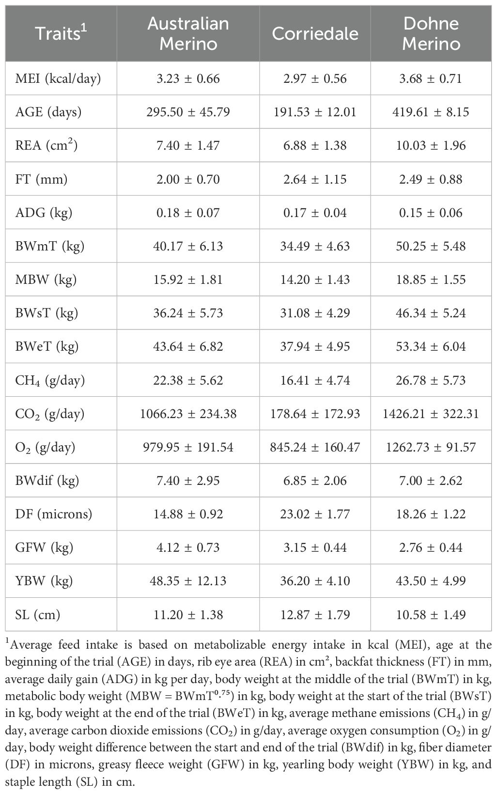
Table 1. General data description presented as the mean ± standard deviation for all traits.

2.4 Feature selection

The feature selection aimed to identify the variables that best explain the MEI in kcal/day. The methods used included track analysis (TA), backward and forward stepwise models (Stepwise), and principal components analysis (PCA). The considered variables were: rib eye area (REA) in cm²; backfat thickness (FT) in mm; average daily gain (ADG) in kg per day; body weight at the middle of the trial (BWmT) in kg; metabolic body weight (MBW = BWmT^0.75) in kg; body weight at the start of the trial (BWsT) in kg; body weight at the end of the trial (BWeT) in kg; average CH₄ emissions in g/day; average CO₂ emissions in g/day; average O₂ consumption in g/day; body weight difference between the start and end of the trial (BWdif) in kg; fiber diameter (DF) in microns; greasy fleece weight (GFW) in kg; weaning body weight (YBW) in kg; and staple length (SL) in cm. Wool traits were evaluated at first shearing of each breed, approximately at 365 days of age, following De Barbieri et al. (2024). The rib eye area (REA) and backfat thickness (FT) were measured using ultrasound at the end of the trial, at the level of the last floating rib, one centimeter from the spine (between the 12th and 13th ribs). All variables were pre-processed in order to standardize the variance considering the trial and the pen, which comprised the contemporaneous group (CG), with the aim of making comparisons between all CGs in the data set, but preserving a data structure not regressed to zero, with values ​​varying only in one direction (positive values). This data processing can be seen in Equation 7:

$\begin{array}{ll}New\_value=\text{ Original}\_\text{value}/\text{CG stander desviation}& (7)\end{array}$

For the training of algorithms and models, the variables selected by the feature selection in the track analysis method, the stepwise model, and principal component analysis (retaining 80% of the cumulative variance) were used as input. All algorithms and models were evaluated using each of these three feature selection approaches.

2.5 Statistics and machine learning algorithms procedures

The dataset used for training the models consisted of 1,177 observations, corresponding to 80% of the initial database (1,472). For cross-validation, this dataset was divided such that one part was used for training and another for testing using the k-fold method. Direct validation was performed on the testing dataset (295 observations), which was not known by the models and corresponds to 20% of the initial database.

Three approaches were used for feature selection: the track analysis method, which utilizes standardized partial regression (Rojo Baio et al., 2019) for data with multicollinearity using the GENES software (Cruz, 2013); the backward and forward stepwise methods of the "stats" R package (R Core Team, 2021); and principal components analysis using the Rbio software (Bhering, 2017).

For a better understanding of the feature selection using the track analysis method, a correlation network was performed using the Rbio software (Bhering, 2017). Afterward, the data underwent a multicollinearity diagnosis, which confirmed a high level of collinearity among the explanatory variables. Consequently, it was particularly considered in the track analysis in GENES. The features selected were those that presented Pearson correlation and direct effect in the same directions, with a direct effect greater than or equal to 0.05.

After running the stepwise feature selection to find the best model, a dominance analysis was performed to investigate the importance of each variable in the model using the "domin" function from the R package "domir" (Luchman, 2023). In the principal components analysis, the principal components (PCs) selected were those that accumulated 80% of the total variance.

The prediction approaches used were the stepwise model, linear regression model, nonlinear regression model, k-nearest neighbor regression model, and random forest regression model from the "mlr" R package (Bischl et al., 2016) as well as support vector machines from the "e1071" R package (Meyer et al., 2023).

The stepwise and linear model (Linear Model) uses the equation of a straight line. The nonlinear regression model employs supervised learning of generalized additive models (Nonlinear Model). The k-nearest neighbor regression model utilizes the k-nearest neighbor's algorithm for regression (k-Nearest Neighbor Model). The random forest regression model relies on tree-based algorithms for regression (Random Forest Model). Lastly, support vector machines (Support Vector Machine) search for a regression function that minimizes the error between predictions, known as support vector regression (Rhys, 2020).

For the k-Nearest Neighbor Model, the k hyperparameter was tuned using cross-validation with k-fold resampling and 20 iterations. To construct the parameter set, we created a description object for a parameter where k ranged from 1 to approximately 34 (the square root of the number of observations in the training set). For the search ranges was used the R function "makeTuneControlGrid()" from "mlr" R package (Bischl et al., 2016). The number of k-nearest neighbors was presented according to the feature selection procedure. For the Random Forest Model, the hyperparameters considered were the number of individual trees in the forest (ranging from 50 to 1000), the number of features to randomly sample at each node (ranging from 100 to 1200), the minimum number of cases allowed in a leaf (ranging from 1 to 20), the maximum number of leaves allowed (ranging from 5 to 100), up to 500 iterations in the random search method, and cross-validation with k-fold resampling and 20 iterations. For the Support Vector Machine, the hyperparameters considered were epsilon (ranging from 0 to 1, in 0.1 increments) and a cost that ranged from 1 to 100. The R scripts for this hyperparameters turning are available in the supplementary materials.

The model training was conducted using cross-validation with k-fold resampling and 20 iterations. The k-fold cross-validation method randomly splits the data into approximately equal-sized subsets called folds. One of these folds is then kept as a test set, while the remaining data is used as the training set. The test set is passed through the model or learning algorithm, and performance metrics – such as R², root mean squared error (RMSE), and Pearson and Spearman correlations – are recorded. Different folds of the data are used as the test set in each iteration, ensuring that all folds have been used once as the test set. The performance metrics reported are the average of all test set runs.

Pearson and Spearman correlations were used as validation metrics in the testing dataset, calculated with the "cor.test" function from the "stats" R package (R Core Team, 2021).

For the confusion matrix calculation for the validation dataset, the observed and predicted MEI were transformed into three classes (low, medium and high MEI). Animals with MEI less than or equal to the 25th percentile were classified as low (the 25% lowest MEI values), those greater than or equal to the 75th percentile were classified as high (the 25% highest MEI values), and those between the 25th and 75th percentiles were classified as medium (values ​​about the average and median of MEI). This classification is analogous to the classification for residual feed intake (Ellison et al., 2019). The confusion matrix was plotted using the "plot_confusion_matrix" function from the "cvms" R package (Olsen, 2021).

3 Results

Pearson correlation and direct effect values obtained by the feature selection using the TA are presented in Table 2. Figure 1 shows the Pearson correlations, highlighting strong and positive relationships among body weight traits (BWsT, BWmT, MBW, and BWeT), gain traits (BWd and ADG), and gases (CO₂ and O₂). These groups exhibited moderate correlation coefficient values with MEI, ranging from 0.41 to 0.59. After identifying these relationships, a multicollinearity diagnosis was performed, and a track analysis method for data with collinearity was used to select the best traits.

Table 2

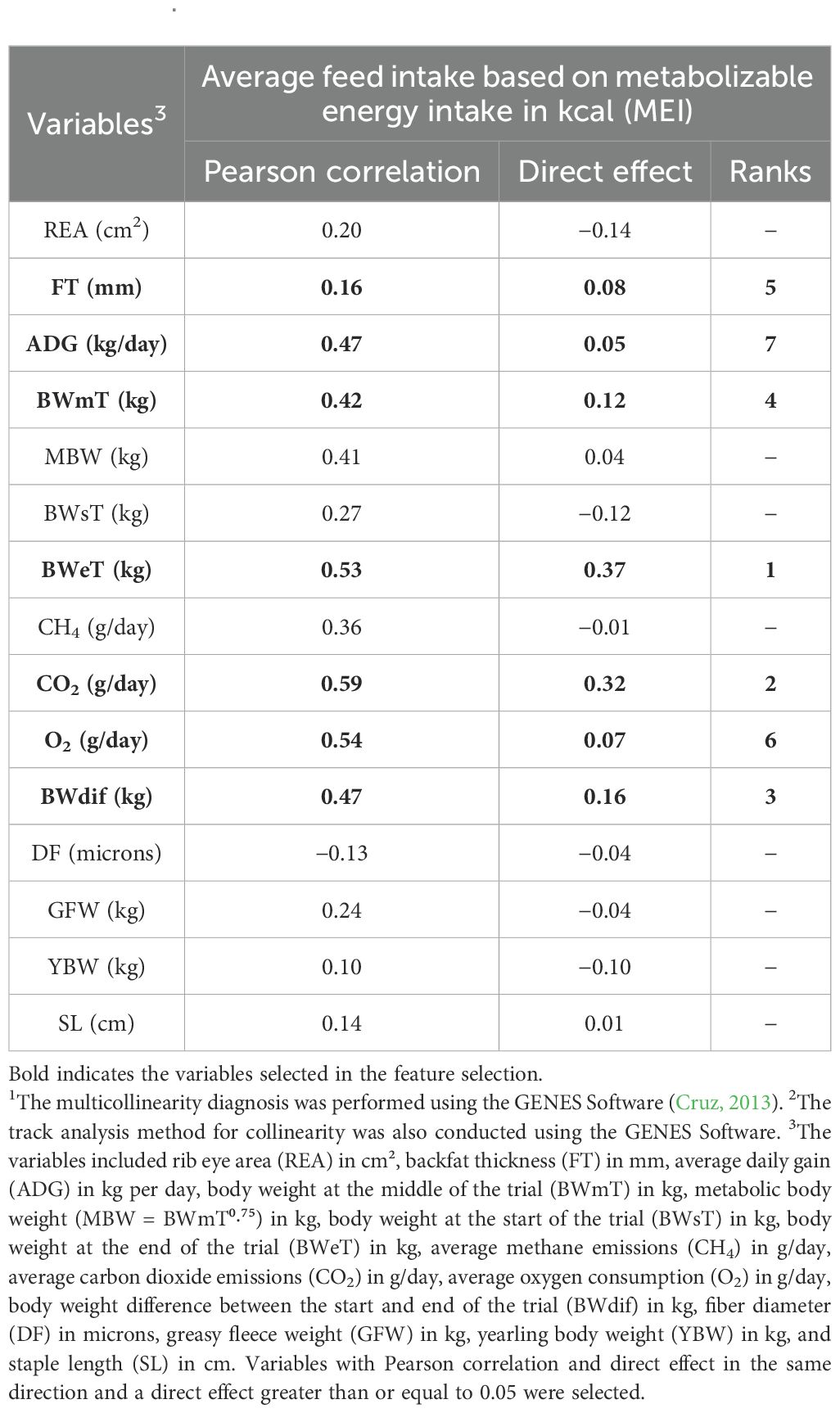
Table 2. Selected variables feature selection using the track analysis method (TA)^1,2.

Figure 1

Figure 1. Pearson Correlation Network between all variables in the dataset, using the software Rbio (Bhering, 2017). The green lines represent positive correlations, while the red lines represent negative correlations. The thickness of the lines indicates the strength of the correlation coefficient, ranging from transparent lines (values close to zero) to thick lines (values close to one). Variables included in the analysis are: average feed intake based on metabolizable energy intake in kcal (MEI); age at the beginning of the trial (AGE) in days; rib eye area (REA) in cm²; fat thickness (FT) in mm; average daily gain (ADG) in kg per day; body weight at the middle of the trial (BWmT) in kg; metabolic body weight (MBW = BWmT⁰·⁷⁵) in kg; body weight at the start of the trial (BWsT) in kg; body weight at the end of the trial (BWeT) in kg; average methane emissions (CH₄) in g/day; average carbon dioxide emissions (CO₂) in g/day; average oxygen consumption (O₂) in g/day; body weight difference between the start and end of the trial (BWd) in kg; fiber diameter (DF) in microns; greasy fleece weight (GFW) in kg; yearling body weight (YBW) in kg; and staple length (SL) in cm.

The variables that presented the same direction of the Pearson correlation and direct effect, with direct effects greater than 0.05, were FT, ADG, BWmT, BWeT, CO₂, O₂, and BWdif. The features that presented the greatest direct effects were BWeT and CO₂, with values of 0.37 and 0.32, respectively, meaning they could explain 37% and 32% of the variation in MEI. The BWdif, BWmT, FT, O₂, and ADG had direct effects of 0.16, 0.12, 0.08, 0.07, and 0.05, respectively.

In the feature selection using the Stepwise model with backward and forward methods, the variables that showed better explanatory capacity were the REA, FT, BWmT, MBW, CH₄, CO₂, BWdif, GFW, DF, and YBW (Table 3). The dominance analysis indicated that the most important trait was CO₂, with a general dominance of 0.156, explaining 15.6% of MEI variation (Rank 1 in Table 3). The second most important trait was BWeT, with a general dominance of 0.097. Other classifications can be seen in Table 3.

Table 3

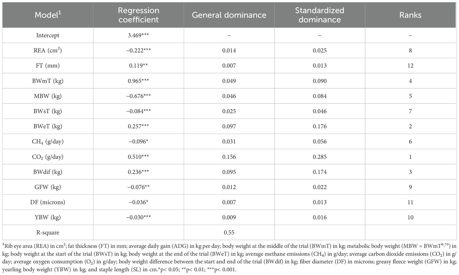
Table 3. Selected variables feature selection using stepwise model with backward and forward (Stepwise) and dominance analysis.

The PCA obtained a cumulative proportion of variance greater than 0.80 in the top six principal components (PCs; Table 4). PC1 had a total variance of 0.338 and only surpassed the 0.70 mark when combined with PC2, PC3, PC4, and PC5. A total of six principal components were needed to obtain a satisfactory proportion of explanation of the total variance.

Table 4

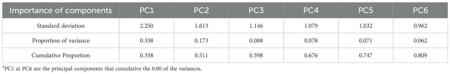
Table 4. Importance of components in the feature selection using the principal components analysis (PCA).

The prediction approaches that presented determination coefficients (R²) greater than or equal to 0.70 were the Random Forest Model using the TA as feature selection (R² = 0.70), k-Nearest Neighbor Model using the PCA as feature selection (R² = 0.72), Random Forest Model using the Stepwise as feature selection (R² = 0.77), Support Vector Machine using the PCA as feature selection (R² = 0.80), Support Vector Machine using the TA as feature selection (R² = 0.82), k-Nearest Neighbor Model using the Stepwise as feature selection (R² = 0.83), and Support Vector Machine using the Stepwise as feature selection (R² = 0.91). The Pearson and Spearman correlation coefficients in these models ranged from 0.84 to 0.95 and 0.78 to 0.93, respectively. Other fit values and hyperparameters can be seen in Table 5.

Table 5

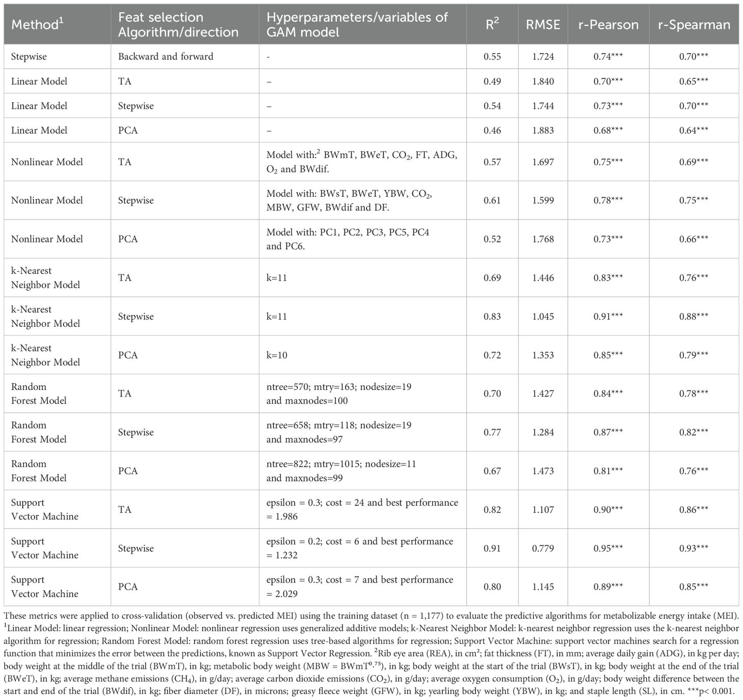
Table 5. Performance metrics: The performance metrics used in this study include R², root mean squared error (RMSE), and Pearson and Spearman correlation coefficients (r).

Pearson and Spearman correlation coefficients of all approaches in the direct validation were greater than 0.60. However, the best models were those that presented values greater than 0.80 for both correlation methods. These were the k-Nearest Neighbor Model using Stepwise and PCA as feature selection with values of 0.92 and 0.90, and 0.86 and 0.81, respectively; the Random Forest Model using TA and Stepwise as feature selection with values of 0.86 and 0.82, and 0.89 and 0.85, respectively; and the support vector using Stepwise as feature selection with values of 0.91 and 0.87 (Table 6).

Table 6

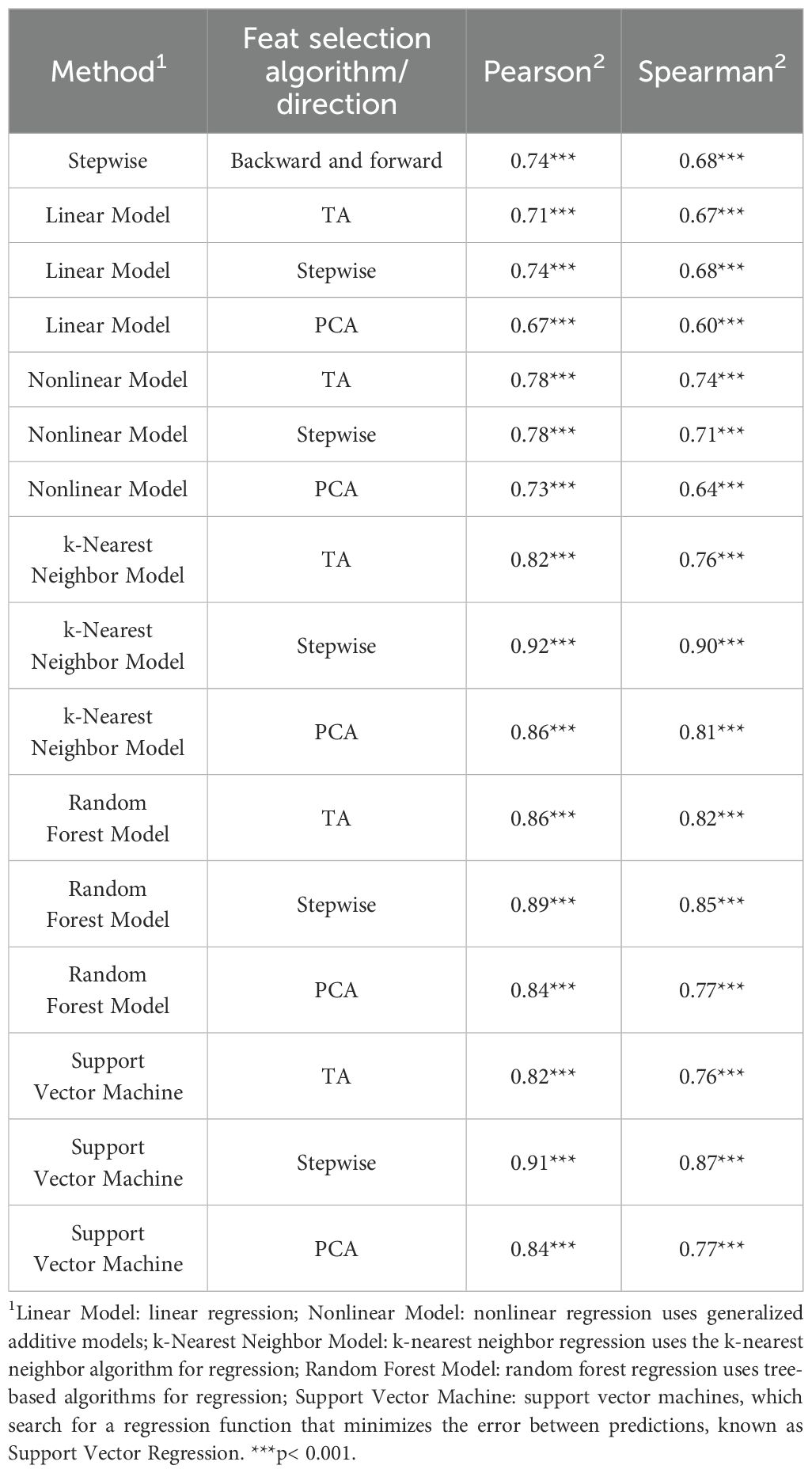
Table 6. Pearson and Spearman correlations coefficients for observed and predict metabolizable energy intakes for testing dataset (n = 295).

The prediction models using TA for feature selection (Figure 2) presented accuracies (Acc) ranging from 0.62 to 0.70 in the confusion matrices. However, only the Nonlinear (Acc = 0.63) and Random Forest (Acc = 0.70) Models did not present confusion between the High and Low MEI classifications. In the Stepwise model for feature selection (Figure 3), the Acc ranged from 0.61 to 0.76, with no confusion between High and Low MEI classification in only the k-nearest neighbor (Acc = 0.74) and support vector (Acc = 0.76) models. The accuracy ranged from 0.53 to 0.71 in PCA feature selection (Figure 4), and the model without confusion between High and Low MEI classification was the k-nearest neighbor (Acc = 0.68).

Figure 2

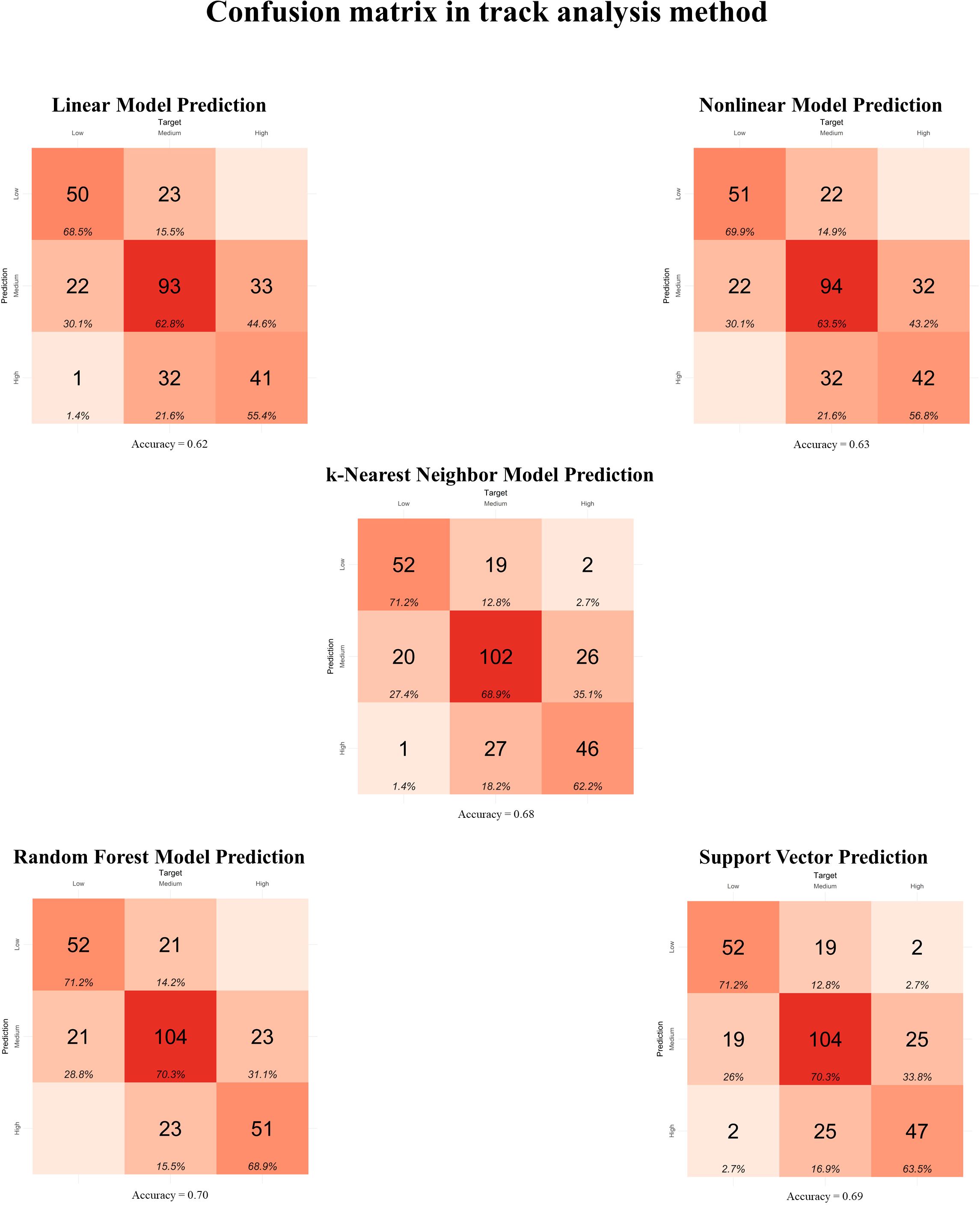
Figure 2. Confusion matrix between observed and predicted metabolizable energy intake (MEI) classifications in the testing dataset (n = 295) for feature selection using the track analysis method. Linear Model: linear regression; Nonlinear Model: nonlinear regression uses generalized additive models; k-Nearest Neighbor Model: k-nearest neighbor regression uses the k-nearest neighbor algorithm for regression; Random Forest Model: random forest regression uses tree-based algorithms for regression; Support Vector: support vector machines search for a regression function that minimizes the error between predictions, known as Support Vector Regression.

Figure 3

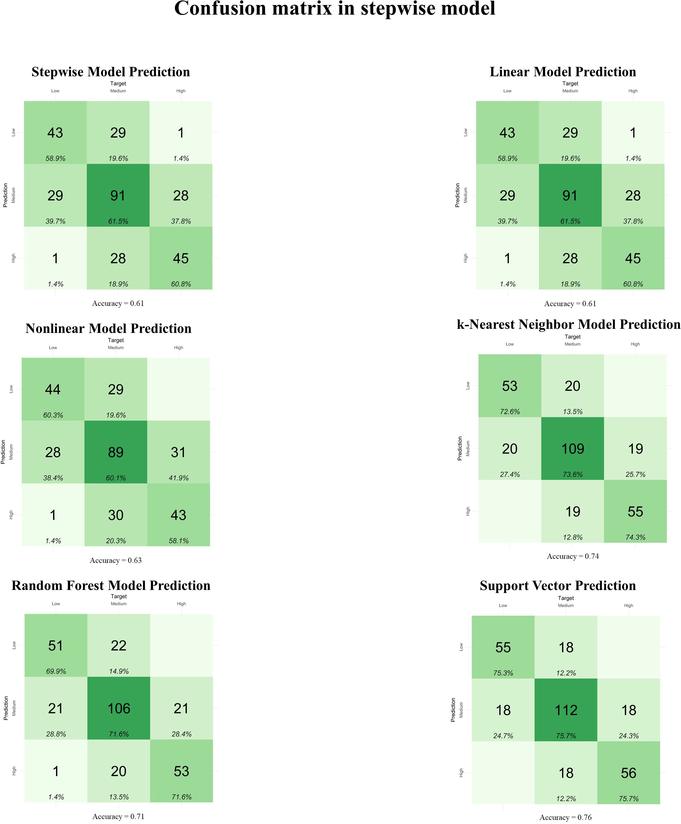
Figure 3. Confusion matrix between observed and predicted metabolizable energy intake (MEI) classifications in the testing dataset (n = 295) for feature selection using the backward and forward stepwise model. Linear Model: linear regression; Nonlinear Model: nonlinear regression uses generalized additive models; k-Nearest Neighbor Model: k-nearest neighbor regression uses the k-nearest neighbor algorithm for regression; Random Forest Model: random forest regression uses tree-based algorithms for regression; Support Vector: support vector machines search for a regression function that minimizes the error between predictions, known as Support Vector Regression.

Figure 4

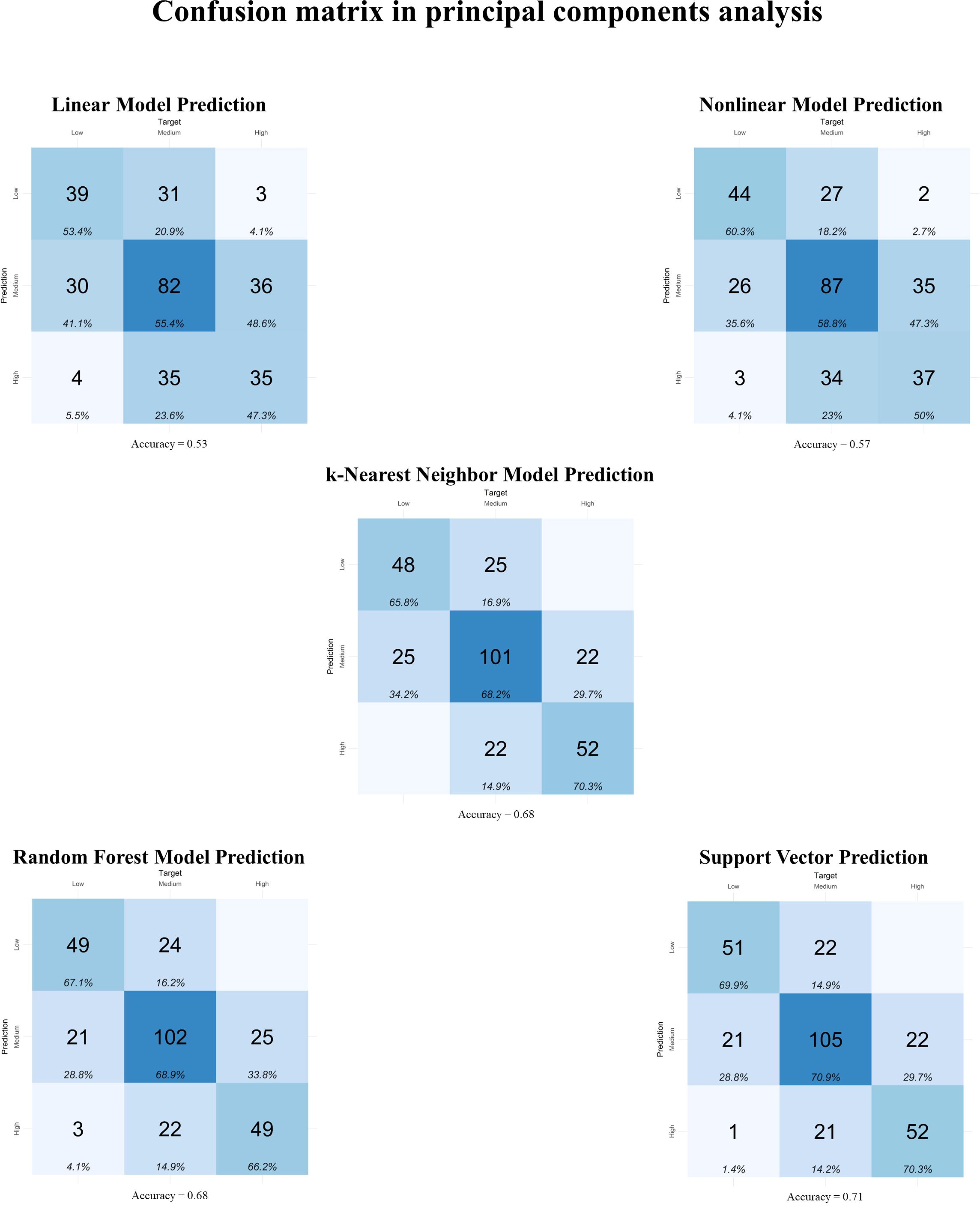
Figure 4. Confusion matrix between observed and predicted metabolizable energy intake (MEI) classifications in the testing dataset (n = 295) for feature selection using principal components analysis. Linear Model: linear regression; Nonlinear Model: nonlinear regression uses generalized additive models; k-Nearest Neighbor Model: k-nearest neighbor regression uses the k-nearest neighbor algorithm for regression; Random Forest Model: random forest regression uses tree-based algorithms for regression; Support Vector: support vector machines search for a regression function that minimizes the error between predictions, known as Support Vector Regression.

4 Discussion

In Uruguayan genetic evaluation, the Australian Merino dataset provides more feed intake information. By aggregating the Corriedale and Dohne Merino information, prediction models can be developed and potentially applied in the future for animals of these breeds. In this context, machine learning approaches can offer valuable generalizations to utilize available information effectively and obtain feed intake data.

The differences in feed intake and gas emissions observed in Table 1 are dependent on several factors. The Corriedale breed showed lower MEI and gas emissions but also had lower growth and final weight because they were evaluated at a younger age (De Barbieri et al., 2024). Although heavier animals had greater MEI, age was the principal factor influencing it. Table 1 indicates that Dohne Merino animals are older and, consequently, heavier with greater gas emissions.

4.1 Feature selection

Feature selection can be understood as the process of choosing variables that best help in understanding data, aiming to reduce computation requirements and dimensionality while consequently improving the performance of the predictors (Chandrashekar and Sahin, 2014). When traits present a high level of redundancy, different feature ranks can be produced in different training samples, resulting in different models with the same prediction accuracy (Piles et al., 2021). In the present study, 15 variables were tested, and seven were selected for the TA, 11 for the Stepwise, and six PCs for the PCA analysis.

The variables selected that could explain the variation in MEI for feature selection reinforce the findings of Tortereau et al. (2020) that productive variables can explain MEI, contradicting the results of Safari et al. (2007) and Fogarty et al. (2009). Methane emissions, which were identified by Donoghue et al. (2015), Robinson and Oddy (2016), and Robinson et al. (2020) as a promising proxy, were selected in the Stepwise feature selection in the present study as a variable with moderate explanatory power of MEI. However, CO₂ emissions were more significant in predicting MEI. This aligns with Arthur et al. (2018), who found that increased feed consumption leads to higher CO₂ production. Renand et al. (2019) mention CO₂ emissions as a potential variable for indirect selection of feed efficiency along with CH₄, when no daily feed intake measurement is available. However, the correlations between CH₄ and CO₂ range from moderate to very strong in Robinson et al. (2016), moderate to strong in Paganoni et al. (2017), and weak to moderate in Jonker et al. (2018). This fact could explain why CO₂ was selected and CH₄ was not in the TA, as one trait could exclude the other due to high redundancy.

The physiological rationale for these observations may stem from the distinct relationships of CO₂ and CH₄ to energy metabolism and digestibility, respectively. Specifically, energy expenditure in animals, driven by the oxidation of organic matter (consuming oxygen and producing carbon dioxide; Arthur et al., 2018), often occurs at the expense of heat production. Conversely, during methane formation, CO₂ acts as a hydrogen sink resulting from microbial fermentation, potentially diverting energy away from the digestion of ingested food. Consequently, a greater intake of substrates, whether in terms of feed quantity or metabolizable energy, leads to increased oxidation of organic matter and a concomitant rise in CO₂ emissions. When this increased substrate availability is coupled with a synchronized rate of microbial degradation, CH₄ emissions also increase. However, in cases of asynchrony between substrate availability and microbial degradation, the excess CO₂ is primarily eliminated through respiration.

Thus, as previously mentioned the CO₂ produced by both ruminal fermentation and oxidation of substrates is proportional to energy expenditure (Hegarty, 2013). CH₄ emission is related to an inefficient digestive process, representing an important loss of feed gross energy (Olijhoek et al., 2018). Therefore, a reduction in gas emissions, due to its relationship with improved digestibility, would consequently also be observed as a decrease in feed intake (Cantalapiedra-Hijar et al., 2018) without necessarily compromising the daily nutrient supply to the animal. Thus, low apparent CO₂ emission could be considered a potential proxy for low feed intake in sheep (Hegarty, 2013), as this variable ranked second and first in the TA and Stepwise feature selection, respectively.

In the study by Bond et al. (2023), a moderate correlation was found between dry matter intake and CH₄ (0.47), measured in respiratory chambers, and a weak correlation with average daily gain (0.28). Similarly, Muir et al. (2020) found phenotypic correlations between dry matter intake, growth rate, and CH₄ emissions in maternal composite ewes of different ages (post-weaning, hogget, and adult). The correlations tended to be greater in post-weaning and adult animals compared to hoggets (0.40, 0.37, and 0.20, respectively). The growth rate showed correlations with dry matter intake in hoggets ranging from 0.17 to 0.42, while in post-weaning and adults, the values were 0.35 and 0.37, respectively. These results indicate that the variables have different relationships with feed intake at various ages. Our study worked with animals of different ages but without repeated measurements in different productive phases. It would be valuable to obtain information related to the entire production cycle and not just a specific phase. However, due to the cost of trials, instead of measuring fewer animals with experimental objectives, the current approach of using data from individuals participating in genetic evaluation may compensate for the absence of repetitions by providing a greater amount of information.

Variables measured during the feed intake test period typically have a significant influence in explaining animal consumption, as observed by Rose et al. (2023), who found phenotypic correlations between feed intake and growth and body weight of 0.52 and 0.46, respectively, during the feed intake test period. This demonstrates the importance of traits measured in this period for predicting intake. Since the proposal by Koch et al. (1963), several studies have analyzed feed intake records in a linear form, considering body weight and body weight gain as covariates to estimate residual feed intake. In Knott et al. (2008), feed intake was modeled using average daily gain (ADG) and live weight in the mid-test. Similarly, studies by Johnson et al. (2017), Zhang et al. (2017), Lima Montelli et al. (2019) and Amarilho-Silveira et al. (2022) adjusted feed intake using ADG and metabolic body weight. Based on these studies, for the estimation of residual feed intake, body weight (or metabolic body weight) and weight gain (BWdif and ADG) are necessary for feed intake prediction. Additionally, these results highlight the importance of feed intake variables in prediction. Blake et al. (2023), using machine learning approaches based on random forest algorithms, identified body weight and average daily gain as the principal proxies for feed intake prediction in beef cattle. In the present study, these variables were selected in the feature selection for TA and Stepwise methods, making them acceptable proxies for MEI prediction.

The principal components (PCs) are the result of the multivariate technique called principal component analysis (PCA). These PCs are orthogonal vectors that point in the direction of the greatest data variability. While the number of PCs is equal to the number of variables, Table 4 only considers PCs that presented cumulative variances of 0.80 or greater. In this way, we did not obtain information on which individual variables contribute to explaining the MEI variation, but the linear combination of these PCs formed new, uncorrelated variables used in the prediction models.

4.2 Metabolizable energy intake prediction

The MEI in the training dataset was predicted using k-fold cross-validation with metrics that enabled predictions with relative confidence. To date, no study has been found using the machine learning approach to predict MEI in sheep. However, linear models for predicting feed intake were used in several studies with R² ranging from 0.33 to 0.84 (Knott et al., 2008; Redden et al., 2011; Cockrum et al., 2013; Johnson et al., 2015; Redden et al., 2014; Johnson et al., 2016; Zhang et al., 2017; Lima Montelli et al., 2019; Tortereau et al., 2020; Amarilho-Silveira et al., 2022; Supplementary Table). Although the approach used in these studies did not include machine learning, their results provide very informative baseline values for prediction models of feed intake. Thus, the results of the present study for the better approaches (Table 5) are between 0.30 and 0.41 points above the recommendation by Johnson et al. (2017) for a model with good explanatory power (R² ≥ 0.70).

In the validation datasets, the greatest Pearson and Spearman correlation coefficients were found using the k-Nearest Neighbor Model, with values of 0.92 and 0.90, respectively. In a study on predicting feed intake of cows, Pearson's correlation coefficients using mixed and machine learning models showed values ranging from 0.71 to 0.76 between actual and predicted feed intake in the test dataset, with lower correlations coefficients in machine learning models when applied on the training dataset (Kamphuis et al., 2017). In the present study, the correlation coefficients were similar in the validation (test) compared to the training dataset. However, only the Linear Model using PCA as feature selection in both the train and test datasets presented Pearson and Spearman correlation coefficients lower than 0.70.

The high coefficient of determination achieved by the SVM using stepwise modeling for feature selection raises a potential risk of overfitting. However, this risk was mitigated in the present study, as evidenced by the consistently high Pearson and Spearman correlation coefficients observed in the validation set. This robust validation performance likely resulted from the implementation of cross-validation, which systematically utilizes distinct subsets of the training data for evaluation. This strategy provides more stable and reliable estimates of model generalization, suggesting good performance on unseen datasets. Had overfitting been detected, further investigations, such as adjusting hyperparameters, the number of k-folds, and repetitions (Rhys, 2020), would have been necessary.

For classifying animals by their Metabolic Efficiency Index (MEI), both the k-Nearest Neighbor Model and Support Vector Machine with stepwise feature selection provide more reliable results. In this context, the use of the confusion matrix, as presented subsequently, can demonstrate this improved performance more reliably within the direct validation dataset (test).

4.3 Confusion matrices

The R² and correlation metrics provided a good indication of the performance of different models. However, to visualize how the animals could be classified and thus extrapolate to practical application, it was proposed to present the results using a confusion matrix. A confusion matrix presents information about how often a given behavior (in the present study, the MEI) is correctly detected and how often it is classified as another behavior (Ruuska et al., 2018).

The confusion matrices for the TA feature selection presented an accuracy greater than or equal to 0.62 for all models, with an emphasis on the Random Forest Model, which presented an accuracy of 0.70 without confusion in the High and Low classifications. In the Stepwise feature selection, the highest accuracy was achieved by the support vector (0.76), followed by the k-nearest neighbor with an accuracy of 0.74, both without confusion between High and Low classifications. For the PCA feature selection, the lowest accuracy was for the Linear Model (0.53), while the highest accuracy was for the support vector (0.71), although there was one observation predicted as High MEI when it was Low. The best performance in the confusion matrix for this feature selection was the k-Nearest Neighbor Model, with an accuracy of 0.68 and no confusion between High and Low classifications.

In the study by Mansbridge et al. (2018) using the Random Forest Model, k-Nearest Neighbor Model, and Support Vector Machine to classify grazing and ruminating behavior in sheep, accuracy ranged from 0.91 to 0.92 for random forest, from 0.79 to 0.87 for k-nearest neighbor, and from 0.67 to 0.73 for support vector machines. The Random Forest Model has shown good potential for predicting feed intake in grazing dairy cattle in the study by Leso et al. (2019). In a lamb survival study, the random forest performed very well in classifying mothering ability with an accuracy of 0.83 (Odevci and Emsen, 2019). In the study by Odevci et al. (2021), the accuracy of the Random Forest Model was 0.83 and 0.93 for mothering ability and lamb survival rate, respectively. In Romney ewes, the body condition score was predicted with an accuracy above 0.88 for pre-breeding, pregnancy diagnosis, pre-lambing, and weaning using the Random Forest Model (Semakula et al., 2021). Therefore, when there is relatively large variation between the training and validation dataset, the Random Forest Model may produce unstable results (Leso et al., 2019). Thus, only in the feature selection with the TA did random forest perform better. However, in the other feature selections, despite high accuracies, this model presented misclassification problems.

The feature selection and cross-validation algorithm combinations that yielded superior direct validation performance on the test set also exhibited higher accuracies in their respective confusion matrices. However, this relationship was not strictly proportional. For instance, despite achieving high Pearson and Spearman correlation coefficients of 0.92 and 0.90 for k-Nearest Neighbors with stepwise feature selection, and 0.91 and 0.87 for support vector with stepwise feature selection, the corresponding accuracies were only 0.74 and 0.76, respectively. This discrepancy likely arose from the unbalanced definition of the low, medium, and high MEI classes, with the medium class alone comprising 50% of the total observations.

The Linear Model exhibited the lowest performance across all feature selection methods. The Nonlinear Model showed high performance with the TA method, average performance with the Stepwise method, and low performance (comparable to the Linear Model) with the PCA method. This fact slightly differs from what is reported in the bibliography, which states that generalized additive models (Nonlinear Model) are sufficiently flexible to capture trends without making strong assumptions about their shapes. Additionally, using substantially fewer parameters, they can adjust a wide variety of shapes of underlying data trends (Borchers et al., 1997). However, the weakness of generalized additive models is that they have a propensity to overfit the training dataset and perform poorly when the validation dataset is outside the range of the training dataset values (Rhys, 2020). Both situations were not observed in the present study.

4.4 Finals comments

The application of cross-validation procedures, both in statistical models and in models based on algorithms that intelligently learn patterns to predict MEI, may also increase the number of animals with this information. For example, if structures for daily feed intake and weight collections are available that allow the collection of a specific number of animals per evaluation period, simple structures with collective feeders and drinkers, where the animals have ad libitum access to feed and water, would be sufficient to phenotype them. In these structures, it would only be necessary to obtain information from the animals such as ultrasonography (rib eye area and fat thickness), weights during the trial period (initial and end weight, weight in the middle trial, and the differences between end and final weight), gas measurements using portable accumulation chambers (CO₂ and CH₄), and genetic evaluation traits (greasy fleece weight, fiber diameter, and yearling body weight). Thus, it would be possible to have a feed intake evaluation center and dispersed test locations where the animals would have access to the same feed as the central test station, with predictor traits independently collected. This setup would enable the evaluation of double the number of animals with feed intake information in each evaluation period.

Even though practically all approaches present excellent R² in cross-validation and correlation coefficients in direct validation, a comprehensive assessment must include the confusion matrix. Therefore, it can be said that the best predictors so far are the k-Nearest Neighbor Model and Support Vector Machine using Stepwise as feature selection. Nevertheless, it is important to note the possibility of overfitting that may have occurred in the support vector, which showed an R² of 0.91 in cross-validation (Table 4). However, according to Montesinos López et al. (2022), when overfitting occurs, the model learns the training data set so well that it performs poorly on unseen data sets, a fact not observed here given the high Pearson and Spearman correlation coefficients in the direct validation dataset.

5 Conclusion

In conclusion, the individual daily metabolizable energy intake (MEI) in Australian Merino, Corriedale, and Dohne Merino sheep can be predicted using the multi-breed dataset with good accuracy using machine learning approaches. The best models for predicting MEI were the k-Nearest Neighbor Model and Support Vector Machine using Stepwise for feature selection. This is supported by the high coefficients of determination in the training database and the strong performance in the validation sets, as evidenced by high correlation coefficients and accuracies in the confusion matrices. These models accurately identify the MEI predictors, enabling the expansion of the number of animals with this characteristic within the same test period.

Data availability statement

The datasets presented in this article are not readily available because legal restrictions apply to their availability. The data were obtained by INIA and are available from the authors with INIA’s permission. Requests to access the datasets should be directed to Ignacio De Barbieri, aWRlYmFyYmllcmlAaW5pYS5vcmcudXk=.

Ethics statement

The animal studies were approved by INIA Animal Ethics Committee (INIA 2018.2). The studies were conducted in accordance with the local legislation and institutional requirements. Written informed consent was obtained from the owners for the participation of their animals in this study.

Author contributions

FA-S: Conceptualization, Data curation, Formal analysis, Investigation, Writing – original draft, Writing – review & editing. IB: Funding acquisition, Investigation, Project administration, Writing – review & editing. EN: Funding acquisition, Methodology, Writing – review & editing. JC: Investigation, Methodology, Writing – review & editing. GC: Conceptualization, Data curation, Funding acquisition, Investigation, Methodology, Writing – review & editing.

Funding

The author(s) declare that financial support was received for the research and/or publication of this article. This study was financed in part by the Coordenação de Aperfeiçoamento de Pessoal de Nível Superior – Brasil (CAPES) – Finance Code 001. The field work and data collection received funding from the European Union's Horizon 2020 research and innovation programme under the Grant Agreement n°772787 (Smarter) and from the Instituto Nacional de Investigación (INIA_CL_38: Rumiar).

Acknowledgments

The dedication, commitment and work of the INIA Tacuarembó and INIA Las Brujas staff is acknowledged, as well as a large number of students (from Uruguay, Brazil, Colombia, France, Mexico) who collaborate while completing their undergraduate or postgraduate work or their international internships. The artificial intelligence tool Microsoft Copilot was used to assist in improving the language and clarity of the text.

Conflict of interest

The authors declare that the research was conducted in the absence of any commercial or financial relationships that could be construed as a potential conflict of interest.

Generative AI statement

The author(s) declare that Generative AI was used in the creation of this manuscript. The artificial intelligence tool Microsoft Copilot [2025] was used to assist in improving the language and clarity of the text.

Publisher’s note

All claims expressed in this article are solely those of the authors and do not necessarily represent those of their affiliated organizations, or those of the publisher, the editors and the reviewers. Any product that may be evaluated in this article, or claim that may be made by its manufacturer, is not guaranteed or endorsed by the publisher.

Supplementary material

The Supplementary Material for this article can be found online at: https://www.frontiersin.org/articles/10.3389/fanim.2025.1579974/full#supplementary-material

References

Amarilho-Silveira F., de Barbieri I., Cobuci J. A., Balconi C. M., de Ferreira G. F., and Ciappesoni G. (2022). Residual feed intake for Australian Merino sheep estimated in less than 42 days of trial. Livest Sci. 258, 104889. doi: 10.1016/j.livsci.2022.104889

Crossref Full Text | Google Scholar

Arthur P. F., Bird-gardiner T., Barchia I. M., Donoghue K. A., and Herd R. M. (2018). Relationships among carbon dioxide, feed intake, and feed efficiency traits in ad. J. Anim. Sci. 96, 4859–4867. doi: 10.1093/jas/sky308

PubMed Abstract | Crossref Full Text | Google Scholar

Beef + Lamb New Zealand (2021). Compendium of New Zealand farm facts 2021. 45th Edn, ed. BEEF + LAMB NEW ZEALAND. Wellington: Beef+Lamb. Available at: www.beeflambnz.com.

Google Scholar

Bhering L. L. (2017). Rbio: A tool for biometric and statistical analysis using the R platform. Crop Breed. Appl. Biotechnol. 17, 187–190. doi: 10.1590/1984-70332017v17n2s29

Crossref Full Text | Google Scholar

Bischl B., Lang M., Kotthoff L., Schratz P., Schiffner J., Richter J., et al. (2016). Machine learning in R. 304. Available at: https://github.com/mlr-org/mlr.

Google Scholar

Blake N. E., Walker M., Plum S., Hubbart J. A., Hatton J., Mata-Padrino D., et al. (2023). Predicting dry matter intake in beef cattle. J. Anim. Sci. 101. doi: 10.1093/jas/skad269

PubMed Abstract | Crossref Full Text | Google Scholar

Bond J. J., Hudson N. J., Khan U. H., Dougherty H. C., Pickford Z., Mackenzie S., et al. (2023). Phenotypic variation in residual feed intake and relationship with body composition traits and methane emissions in growing wether lambs. Anim. Prod Sci. 63, 1705–1715. doi: 10.1071/AN22425

Crossref Full Text | Google Scholar

Borchers D. L., Buckland S. T., Priede I. G., and Ahmadi S. (1997). Improving the precision of the daily egg production method using generalized additive models. Can. J. Fisheries Aquat. Sci. 54, 2727–2742. doi: 10.1139/f97-134

Crossref Full Text | Google Scholar

Cantalapiedra-Hijar G., Abo-Ismail M., Carstens G. E., Guan L. L., Hegarty R., Kenny D. A., et al. (2018). Review: Biological determinants of between-animal variation in feed efficiency of growing beef cattle. Animal 12, S321–S335. doi: 10.1017/S1751731118001489

PubMed Abstract | Crossref Full Text | Google Scholar

Chandrashekar G. and Sahin F. (2014). A survey on feature selection methods. Comput. Electrical Eng. 40, 16–28. doi: 10.1016/j.compeleceng.2013.11.024

Crossref Full Text | Google Scholar

Charmley E., Williams S. R. O., Moate P. J., Hegarty R. S., Herd R. M., Oddy V. H., et al. (2016). A universal equation to predict methane production of forage-fed cattle in Australia. Anim. Prod Sci. 56, 169–180. doi: 10.1071/AN15365

Crossref Full Text | Google Scholar

Cockrum R. R., Stobart R. H., Lake S. L., and Cammack K. M. (2013). Phenotypic variation in residual feed intake and performance traits in rams. Small Ruminant Res. 113, 313–322. doi: 10.1016/j.smallrumres.2013.05.001

Crossref Full Text | Google Scholar

Cruz C. D. (2013). GENES - Software para análise de dados em estatística experimental e em genética quantitativa. Acta Sci. Agron. 35, 271–276. doi: 10.4025/actasciagron.v35i3.21251

Crossref Full Text | Google Scholar

De Barbieri I., Navajas E. A., Ramos Z., Ferreira G., Velazco J., and Ciappesoni G. (2024). Feed conversion efficiency does not negatively affect young sheep and ewe performance. Front. Anim. Sci. 5, 1480928. doi: 10.3389/fanim.2024.1480928

Crossref Full Text | Google Scholar

Dillon E., Moran B., and Donnellan T. (2021). Teagasc national farm survey 2020: preliminary results. ed. Agricultural Economics and Farm Surveys Department. Carlow: Teagasc.

Google Scholar

Dominik S., Robinson D. L., Donaldson A. J., Cameron M., Austin K. L., and Oddy V. H. (2017). Relationship between feed intake, energy expenditure and methane emissions: implications for genetic evaluation. Proc. Assoc. Advmt. Anim. Breed. Genet. 22, 65–68.

Google Scholar

Donoghue K. A., Bird-Gardiner T. L., Arthur P. F., Herd R. M., and Hegarty R. F. (2015). Genetic parameters for methane production and relationships with production traits in Australian beef cattle. Proc. Assoc. Advmt. Breed. Genet. 21, 114–117.

Google Scholar

Ellison M. J., Conant G. C., Lamberson W. R., Austin K. J., Van Kirk E., Cunningham H. C., et al. (2019). Predicting residual feed intake status using rumen microbial profiles in ewe lambs. J. Anim. Sci. 97, 2878–2888. doi: 10.1093/jas/skz170

PubMed Abstract | Crossref Full Text | Google Scholar

Evaluaciones Genéticas Ovinas (2025). Razas. Available online at: https://www.geneticaovina.com.uy (Accessed April 28, 2025).

Google Scholar

Fogarty N. M., Safari E., Mortimer S. I., Greeff J. C., and Hatcher S. (2009). Heritability of feed intake in grazing Merino ewes and the genetic relationships with production traits. Anim. Prod Sci. 49, 1080–1085. doi: 10.1071/AN09075

Crossref Full Text | Google Scholar

Fogarty E. S., Swain D. L., Cronin G. M., Moraes L. E., and Trotter M. (2020). Behaviour classification of extensively grazed sheep using machine learning. Comput. Electron Agric. 169, 105175. doi: 10.1016/j.compag.2019.105175

Crossref Full Text | Google Scholar

Giorello D., De Barbieri I., Aguerre J. I., Banchero G., Rovira F., Rodriguez B., et al. (2021). Feedlot forrajero: Confinamiento estratégico de corderos con forraje conservado. Rev. INIA Uruguay 68, 12–16.

Google Scholar

Goopy J. P., Robinson D. L., Woodgate R. T., Donaldson A. J., Oddy V. H., Vercoe P. E., et al. (2016). Estimates of repeatability and heritability of methane production in sheep using portable accumulation chambers. Anim. Prod Sci. 56, 116–122. doi: 10.1071/AN13370

Crossref Full Text | Google Scholar

Goopy J. P., Woodgate R., Donaldson A., Robinson D. L., and Hegarty R. S. (2011). Validation of a short-term methane measurement using portable static chambers to estimate daily methane production in sheep. Anim. Feed Sci. Technol. 166–167, 219–226. doi: 10.1016/j.anifeedsci.2011.04.012

Crossref Full Text | Google Scholar

Hegarty R. S. (2013). Applicability of short-term emission measurements for on-farm quantification of enteric methane. Animal 7, 401–408. doi: 10.1017/S1751731113000839

PubMed Abstract | Crossref Full Text | Google Scholar

Johnson P., Miller S., and Knowler K. (2015). Towards a data set to investigate feed efficiency in New Zealand maternal sheep. Proc. Assoc. Advancement Anim. Breed. Genet. 106–109.

Google Scholar

Johnson P. L., Miller S. P., and Knowler K. (2016). Preliminary investigations into the trait of residual energy intake in sheep. NZ Soc. Anim. Prod Proc. 76, 34–37. doi: 10.1079/BJN19660078

PubMed Abstract | Crossref Full Text | Google Scholar

Johnson P. L., Wing J., and Knowler K. (2017). Relationship between measures of residual energy intake made on growing animals and adults. NZ Soc. Anim. Prod Proc. 77, 85–87. doi: 10.1079/BJN19660078

PubMed Abstract | Crossref Full Text | Google Scholar

Jonker A., Hickey S., McEwan J., and Waghorn G. (2020). “Portable accumulation chambers for enteric methane determination in sheep,” in Guidelines for estimating methane emissions from individual ruminants using: GreenFeed, “sniffers”, hand-held laser detector and portable accumulation chamber. Eds. Jomker A. and Waghorn G. C., 49–56.

Google Scholar

Jonker A., Hickey S. M., Rowe S. J., Janssen P. H., Shackell G. H., Elmes S., et al. (2018). Genetic parameters of methane emissions determined using portable accumulation chambers in lambs and ewes grazing pasture and genetic correlations with emissions determined in respiration chambers. J. Anim. Sci. 96, 3031–3042. doi: 10.1093/jas/sky187

PubMed Abstract | Crossref Full Text | Google Scholar

Kamphuis C., van Riel J. W., Veerkamp R. F., and de Mol R. M. (2017). “Traditional mixed linear modelling versus modern machine learning to estimate cow individual feed intake,” in Precision livestock farming ‘17. Eds. Berckmans D. and Keita A. (8th European Conference on Precision Livestock Farming, Nates), 366–376.

Google Scholar

Knott S. A., Cummins L. J., Dunshea F. R., and Leury B. J. (2008). The use of different models for the estimation of residual feed intake ( RFI ) as a measure of feed efficiency in meat sheep. Anim. Feed Sci. Technol. 143, 242–255. doi: 10.1016/j.anifeedsci.2007.05.013

Crossref Full Text | Google Scholar

Koch R. M., Swiger L. A., Chambers D., and Gregory K. E. (1963). Efficiency of feed use in beef cattle. J. Anim. Sci. 22, 486–494. doi: 10.2527/jas1963.222486x

Crossref Full Text | Google Scholar

Leahy S., Clark H., and Reisinger A. (2020). Challenges and prospects for agricultural greenhouse gas mitigation pathways consistent with the paris agreement. Front. Sustain Food Syst. 4. doi: 10.3389/fsufs.2020.00069

Crossref Full Text | Google Scholar

Leso L., Werner J., McSweeney D., Kennedy E., Geoghegan A., and Shalloo L. (2019). “Random forest regression for estimating dry matter intake of grazing dairy cows,” in Precision livestock farming ‘19. Eds. O’Brien B., ShallooThe, Hennessy D., and Shalloo L. (The 9th European Conference on Precision Livestock Farming, Cork), 606–612.

Google Scholar

Lima Montelli N. L. L., Almeida A. K., Ribeiro C.R.de F., Grobe M. D., Abrantes M. A. F., et al. (2019). Performance, feeding behavior and digestibility of nutrients in lambs with divergent efficiency traits. Small Ruminant Res. 180, 50–56. doi: 10.1016/j.smallrumres.2019.07.016

Crossref Full Text | Google Scholar

Luchman J. (2023). Tools to support relative importance analysis. Psychol. Methods 8, 1–19. doi: 10.1037/1082-989X.8.2.129

PubMed Abstract | Crossref Full Text | Google Scholar

Mansbridge N., Mitsch J., Bollard N., Ellis K., Miguel-Pacheco G. G., Dottorini T., et al. (2018). Feature selection and comparison of machine learning algorithms in classification of grazing and rumination behaviour in sheep. Sensors (Switzerland) 18, 1–19. doi: 10.3390/s18103532

PubMed Abstract | Crossref Full Text | Google Scholar

McLeod A. (2011). World livestock 2011 (Rome: Food and Agriculture Organization of the United Nations (FAO).

Google Scholar

Meyer D., Dimitriadou E., Hornik K., Weingessel A., Leisch F., Chang C.-C., et al. (2023). Misc functions of the department of statistics, probability theory group (Formerly: E1071), TU wien. 67. https://CRAN.R-project.org/package=e1071.

Google Scholar

Montesinos López O. A., Montesinos López A., and Crossa J. (2022). “Overfitting, model tuning, and evaluation of prediction performance,” in Multivariate statistical machine learning methods for genomic prediction (Springer International Publishing, Cham), 109–139. doi: 10.1007/978-3-030-89010-0_4

Crossref Full Text | Google Scholar

Muir S. K., Linden N., Kennedy A., Knight M. I., Paganoni B., Kearney G., et al. (2020). Correlations between feed intake, residual feed intake and methane emissions in Maternal Composite ewes at post weaning, hogget and adult ages. Small Ruminant Res. 192. doi: 10.1016/j.smallrumres.2020.106241

Crossref Full Text | Google Scholar

Odevci B. B. and Emsen E. (2019). “Machine learning model for maternal quality in sheep,” in Precision livestock farming ‘19. Eds. O’Brien B., Hennessy D., and Shalloo L. (The 9th European Conference on Precision Livestock Farming, Cork), 69–73.

Google Scholar

Odevci B. B., Emsen E., and Aydin M. N. (2021). Machine learning algorithms for lamb survival. Comput. Electron Agric. 182, 105995. doi: 10.1016/j.compag.2021.105995

Crossref Full Text | Google Scholar

Olijhoek D. W., Løvendahl P., Lassen J., Hellwing A. L. F., Höglund J. K., Weisbjerg M. R., et al. (2018). Methane production, rumen fermentation, and diet digestibility of Holstein and Jersey dairy cows being divergent in residual feed intake and fed at 2 forage-to-concentrate ratios. J. Dairy Sci. 101, 9926–9940. doi: 10.3168/jds.2017-14278

PubMed Abstract | Crossref Full Text | Google Scholar

Olsen L. R. (2021). Cross-validation for model selection - CRAN. 1–100. https://CRAN.R-project.org/package=cvms.

Google Scholar

Paganoni B., Rose G., Macleay C., Jones C., Brown D. J., Kearney G., et al. (2017). More feed efficient sheep produce less methane and carbon dioxide when eating high-quality pellets. J. Anim. Sci. 95, 3839. doi: 10.2527/jas2017.1499

PubMed Abstract | Crossref Full Text | Google Scholar

Pew Research Center (2014). Attitudes about aging: A global perspective. Available at: http://www.pewglobal.org/2014/01/30/attitudes-about-aging-a-global-perspective/.

Google Scholar

Piles M., Bergsma R., Gianola D., Gilbert H., and Piles M. (2021). Feature selection stability and accuracy of prediction models for genomic prediction of residual feed intake in pigs using machine learning. Front. Genet. 12. doi: 10.3389/fgene.2021.611506

PubMed Abstract | Crossref Full Text | Google Scholar

R Core Team (2021). R: A language and environment for statistical computing. https://www.R-project.org.

Google Scholar

Redden R. R., Surber L. M. M., Grove A. V., and Kott R. W. (2014). Effects of residual feed intake classification and method of alfalfa processing on ewe intake and growth. J. Anim. Sci. 92, 830–835. doi: 10.2527/jas.2013-6768

PubMed Abstract | Crossref Full Text | Google Scholar

Redden R. R., Surber L. M. M., Roeder B. L., Nichols B. M., Paterson J. A., and Kott R. W. (2011). Residual feed efficiency established in a post-weaning growth test may not result in more efficient ewes on the range. Small Ruminant Res. 96, 155–159. doi: 10.1016/j.smallrumres.2010.12.007

Crossref Full Text | Google Scholar

Renand G., Decruyenaere V., Maupetit D., and Dozias D. (2019). Methane and Carbon Dioxide Emission of Beef Heifers in Relation with Growth and Feed E ffi ciency. Animals 3, 1–17. doi: 10.3390/ani9121136

PubMed Abstract | Crossref Full Text | Google Scholar

Rhys H. I. (2020). Machine Learning with R, the tidyverse and mlr. 1st Edn. Eds. Michaels M., Warren D., Dragosavljevic A., Weidert L., and Taylor T. (Shelter Island: Manning).

Google Scholar

Robinson D. L., Cameron M., Donaldson A. J., Dominik S., and Oddy V. H. (2016). One-hour portable chamber methane measurements are repeatable and provide useful information on feed intake and efficiency. J. Anim. Sci. 94, 4376–4387. doi: 10.2527/jas2016-0620

PubMed Abstract | Crossref Full Text | Google Scholar

Robinson D. L., Dominik S., Donaldson A. J., and Oddy V. H. (2020). Repeatabilities, heritabilities and correlations of methane and feed intake of sheep in respiration and portable chambers. Anim. Prod Sci. 60, 880–892. doi: 10.1071/AN18383

Crossref Full Text | Google Scholar

Robinson D. L., Goopy J. P., Hegarty R. S., Oddy V. H., Thompson A. N., Toovey A. F., et al. (2014). Genetic and environmental variation in methane emissions of sheep at pasture. J. Anim. Sci. 92, 4349–4363. doi: 10.2527/jas.2014-8042

PubMed Abstract | Crossref Full Text | Google Scholar

Robinson D. L. and Oddy V. H. (2016). Benefits of including methane measurements in selection strategies. J. Anim. Sci. 94, 3624–3635. doi: 10.2527/jas2016-0503

PubMed Abstract | Crossref Full Text | Google Scholar

Rojo Baio F. H., Antuniassi U. R., Castilho B. R., Teodoro P. E., and da Silva E. E. (2019). Factors affecting aerial spray drift in the Brazilian Cerrado. PloS One 14. doi: 10.1371/journal.pone.0212289

PubMed Abstract | Crossref Full Text | Google Scholar

Rose G., Paganoni B., Macleay C., Jones C., Brown D. J., Kearney G., et al. (2023). Methane, growth and carcase considerations when breeding for more efficient Merino sheep production. Animal 17. doi: 10.1016/j.animal.2023.100999

PubMed Abstract | Crossref Full Text | Google Scholar

Ruuska S., Hämäläinen W., Kajava S., Mughal M., and Matilainen P. (2018). Evaluation of the confusion matrix method in the validation of an automated system for measuring feeding behaviour of cattle. Behav. Processes 148, 56–62. doi: 10.1016/j.beproc.2018.01.004

PubMed Abstract | Crossref Full Text | Google Scholar

Safari E., Fogarty N. M., Mortimer S. I., Greeff J. C., Hatcher S., Lee G. J., et al. (2007). Feed intake and its genetic relationship with growth traits in merino sheep. Proc. Assoc. Advmt. Anim. Breed. Genet. 17, 199–202.

Google Scholar

Semakula J., Corner-thomas R. A., Morris S. T., Blair H. T., and Kenyon P. R. (2021). Application of machine learning algorithms to predict body condition score from liveweight records of mature romney ewes. Agric. (Switzerland) 11, 1–22. doi: 10.3390/agriculture11020162

Crossref Full Text | Google Scholar

Shahinfar S. and Kahn L. (2018). Machine learning approaches for early prediction of adult wool growth and quality in Australian Merino sheep. Comput. Electron Agric. 148, 72–81. doi: 10.1016/j.compag.2018.03.001

Crossref Full Text | Google Scholar

Tortereau F., Marie-Etancelin C., Weisbecker J.-L., Marcon D., Bouvier F., Moreno-Romieux C., et al. (2020). Genetic parameters for feed efficiency in Romane rams and responses to single-generation selection. Animal 14, 681–687. doi: 10.1017/S1751731119002544

PubMed Abstract | Crossref Full Text | Google Scholar

Zhang X., Wang W., Mo F., La Y., Li C., and Li F. (2017). Association of residual feed intake with growth and slaughtering performance, blood metabolism, and body composition in growing lambs. Sci. Rep. 7, 1–11. doi: 10.1038/s41598-017-13042-7

PubMed Abstract | Crossref Full Text | Google Scholar