Abstract
When moving from a very sheltered aquaculture site to a very exposed oceanic aquaculture site, the energy increases proportionally in a continuum. Lojek et al. (in review) considered the primary influential parameters (water current, wave height, wave period, wavelength and water depth) which influence the species, structure, technology, methods, and operational aspects of any aquaculture endeavour and investigated six possible indices which cover these variables. Added to advanced computer modelling, assisted by detailed and constant environmental monitoring, it may be possible to refine site selection, structure selection and design, species selection, equipment and logistic requirements and health and safety requirements. This manuscript has selected two indicative indices: Specific Exposure Energy (SEE) index and Exposure Velocity (EV) index from the potential equations provided by Lojek et al. (in review) and compared them with known operational aquaculture sites highlighting present structural capability and limitations. The two indices are also utilized to reflect on their suitability for assessing sample sites with respect to biological, technological, operational or maintenance aspects of aquaculture activities. The indices have shown themselves to be useful tools in the general assessment of the energy that will influence the species and structure selection at potential aquaculture sites. This information can help prospective fish farmers characterize their sites concisely and accurately to consultants, regulators, equipment vendors, and insurance brokers.
1 Introduction
Physical ocean energy is the main characteristic defining accessibility of any potential aquaculture site, as this dictates the feasibility of aquaculture in general as well as the species and the technology most appropriate for the site. Traditionally, aquaculture has been carried out in low energy, sheltered coastal and estuarine habitats (Olsen et al., 2008; Buck et al., 2024). Aquaculture has been increasing significantly worldwide over the last 40 years (FAO, 2022) in terms of the range of species, the quantity produced and the locations where aquaculture takes place. During this period, there has also been an increase in other stakeholder activities, which are in competition for the water space, especially in the coastal sea (Galparsoro et al., 2020). In addition, anthropogenic inputs have also had an influence on the quality of water at inshore and sheltered sites and more and more coastal waters are subject to special utilisation permits and are often declared worthy of protection, e.g. the establishment of marine protected areas (MPAs) (Rodriguez-Rodrıguez et al., 2015), which often excludes use for aquaculture.
Therefore, there has been an increasing trend to extend aquaculture into water bodies off the coast, referred to as offshore or open ocean aquaculture (FAO, 2022). However, we now know that it is not the distance from the coast, but rather the degree of exposure that determines the form of aquaculture that can be undertaken at a site (Buck et al., 2024; Lojek et al., in review1; Sclodnick et al., in review2). Nutrient concentrations in the water column vary locally and seasonally, but in many regions decrease with increasing distance from the coast (Painter et al., 2018). The advantages of these areas are that the water bodies have more stable conditions with regard to changes in temperature, oxygen content, pH and other abiotic factors, which are important particularly in view of future climate change (Ahmed et al., 2019). In addition, grazing/predation pressure is reduced, and biofouling decreases since predators and fouling organisms diminish with distance from the shore and with increasing exposure (Atalah et al., 2016; Visch et al., 2020; Morro et al., 2021).
A longstanding issue which has an influence on the understanding and progress into exposed sites is the terminology used to describe these exposed ocean locations. Other papers of this special edition (Buck et al., 2024; Dewhurst et al., in review3; Heasman et al., in review4; Lojek et al., in review1; Markus, in review5; Sclodnick et al., in review2) have investigated this aspect in some depth, but it is of value to outline the parameters here. The terminology used above and in other manuscripts (Froehlich et al., 2017; Morro et al., 2021) can vary in interpretation leading to misunderstanding of the locations, aquaculture technology, species, and logistic requirements. The main characteristics and their implications are found in Figure 1.
Figure 1

Comparison of “Sheltered” vs. “Exposed” (top) as well as “near to the land” (nearshore) vs. “far from land” (offshore) (bottom) environments along with a selected collection of general and specific descriptions of each (modified after Buck et al., 2024).
However, these descriptions are still relatively undefined in terms of the differences in requirements of these locations (Buck et al., 2024). Extending into high-energy zones found at exposed marine sites necessitates a combination of new thinking; new design; new technology; new materials; and new methods and not limited to making inshore structures bigger and stronger. (e.g. shellfish dropper lines; Gieschen et al., 2020; Landmann et al., 2021). Also, logistics, operation and maintenance as well as health and safety will have to be considered and advanced appropriately to enable a safe and viable enterprise. The question also arises as to whether the current technologies are the right ones to be used in high-energy environments. Perhaps a paradigm shift is needed in the expansion of aquaculture operations into exposed waters. This requires a clear understanding of the requirements for new technologies, and thus the categorisation of a water body in terms of the level of energy. Hence the investigation into the applicability of the indices established by Lojek et al. (in review)1 to quantify the parameters and classification that inform the enquirer as to what technology and procedures are required for different forms of aquaculture and locations.
This alternative would contribute significantly to this classification issue by measuring the amount of exposure (at a worst-case scenario) found at any one point in the water column at a selected location. If the influence of various parameters which essentially indicate the amount of energy found at a site can be determined in a continuum from 0, in a very sheltered site, to a maximum in very exposed seas, then an aquaculture assessment of equipment, species, risk, amongst other variables, can be matched to those sites.
This manuscript investigates the parameters that influence exposure found at a site and also the potential of the exposure indices to support aquaculture farm location, aquaculture species selection and diversification, planning, equipment requirements, operational advancement and health and safety based on information from exiting farm operations.
It should be noted that this manuscript is one of a suite of papers comprising a special edition “Differentiating and defining ‘exposed’ and ‘offshore’ aquaculture and applications for aquaculture operation, management, costs, and policy”. The special edition includes manuscripts focused on aquaculture policy and regulation in marine environments, the definitions of terms regarding aquaculture in marine systems, the derivation of the energy indices, trends required to advance aquaculture into high energy marine zones, costs and implications in aquaculture of using the indices and social science aspects relating to marine aquaculture (Buck et al., 2024).
2 Methods
2.1 Utilisation of indices
The equations which provide a reference value (index) postulated by Lojek et al. (in review)1 are assessed and considered in view of their sensitivities to various hydrodynamic energies and how they represent the sites where known aquaculture takes place. Indices that appear to be sensitive to wave height, water depth, and water currents, which are perceived to be the most influential parameters of water energy at a marine site, are used in case studies. Six indices (A–F) were proposed in Lojek et al. (in review)1, and for the sake of completeness these are summarized in Table 1.
Table 1
| No. | Index | Abbr. | Formula |
|---|---|---|---|
| A | Specific exposure energy index | SEE | |
| B | Exposure velocity index | EV | |
| C | Exposure velocity at reference depth index | EVRD | |
| E | Depth-integrated energy flux index | DEF | |
| E | Structure-centered depth-integrated energy index | SDE | |
| F | Structure-centered drag-to-buoyancy ratio index | SDBR |
List of indexes developed by Lojek et al. (in review)1 for the application of aquaculture sites in high-energy environments.
Since all of these indices were analysed in detail in Lojek et al. (in review)1, we limit ourselves to those indices that include the parameters important for aquaculture, namely water depth (d), horizontal water current (Uc), and wave environment (i.e. height Hs, period Tp, direction, and wave-induced horizontal velocity magnitude uw). The selection of these parameters is based on a list of the most important oceanographic parameters for open ocean as stipulated in Buck and Grote (2018), Buck et al. (2024) and Lojek et al. (in review)1. An assessment of these indices and their application has shown that two indices, namely the Specific Exposure Energy (SEE) index and Exposure Velocity (EV) index, were considered to be the most sensitive and responsive to the parameters describing an exposed location providing clearly distinguishable results as seen in Table 1. The derivation of the indices is covered in Lojek et al. (in review)1 so this manuscript will only focus on the use of the selected indices.
Case studies will follow showing the positioning in the water column of already existing commercial operational sites and how the two indices SEE and EV will respond when using the sites parameter characteristics (see Section 3). All assessments were taken to be at the surface as this is the most conservative measurement and covers the culture of seaweed which must be done at, or very near to, the surface. Further, evaluation of the SEE and EV in these assessments make the simplifying and conservative assumption that the horizontal water current velocity and wave direction are aligned. As such, Uc(z) and uw(z) can be considered magnitudes, referred to as the current speed and the wave-induced horizontal velocity magnitude. In alternative applications of the SEE and EV, the directionality of Uc(z) and uw(z) can be considered.
The manuscript is focused on quantifying exposure as opposed to quantifying energy resources; therefore, it will assist both aquaculture and wave energy site assessments, but it will not define the energy resources per se that would be required for defining power outputs of specific wave or current energy systems.
An index calculator can be found online6 which will allow the reader to use the calculator to generate an index for prospective aquaculture sites.
2.2 The influence of depth on wave motion
Water depth is of significant importance at an aquaculture site as it will have a substantial impact on the wave environment and therefore the energy at an aquaculture site. This energy potential in turn influences the farm technologies installed there, the aquaculture species candidates, as well as the daily routines such as operations and maintenance (O&M). Figure 2 shows the dependence of wave induced water movement on decreasing depth from the open ocean to the coast at different locations: (A) deep water (B) intermediate water, and (C) shallow water (Lojek et al., in review)1.
Figure 2

The relationship between wave height, form and water depth in (A) deep, (B) intermediate, and (C) shallow water wave environments, as characterized by the water depth (d) to wave length (L) ratio. Wave orbital velocity amplitudes and particle displacements underneath a progressive wave transform as d becomes small relative to L. Relevant variables include: z = vertical location in the water column, x = direction of wave propagation, uw(z) = wave-induced horizontal velocity magnitude, Hs = wave height, m.s.l. = mean sea level, Tp = wave period, d = depth, ds = depth of farm structure below surface, Uc = current speed. (Modified after Lojek et al., in review)1.
Dynamically, as a wave approaches shallow water, wave heights increase and the speed at which the wave travels forward decreases (i.e. wave period remains constant and wavelength decreases). Beneath the water surface, waves induce the periodic movement of water particles; from deep to shallow water, these paths transition from circular to elliptical to nearly horizontal. The wave-induced horizontal velocity magnitude decays rapidly with water depth in deep water yet remains constant with water depth in shallow water—resulting in oscillating currents that extend over the entire water column (Figure 2). Finally, wave breaking initiates when the wave-induced velocity at the crest of the wave is greater than the wave speed. These processes show how wave induced velocities below the surface intensify with decreasing water depth (Dean and Dalrymple, 1991). For the aquaculture site, this often means that the total energy that an aquaculture structure is exposed to increases with decreasing depth, impacting the performance, operation and safety of the farm.
Since the interaction of the parameters water depth (d), wave height (Hs), wave period (Tp), current speed (Uc), and the position of the farm in the water column (ds) is of great importance for the understanding of an index application, we will discuss the basics of this interaction in Figures 3, 4 and in Table 2. Figure 3 shows the dependence of an energy potential at a certain location (represented by a freely selectable index, e.g. EV or SEE) on the wave height (Hs) and the current speed at a given wave period (Tp). The parameters are indicated without numbers to give a basic understanding of the shape of the surface graph. The arrows parallel to the wave height axis, current speed axis, and index axis indicate the direction of the increasing values. The colour on the surface corresponds to the index value, which increases with progressive red-dark colouring. It can be clearly seen how the index value depends on the current speed and wave height for a given wave period. If current speed or wave height increases or the wave period decreases, there is also a corresponding increase in the index value. This phenomenon always applies and can be understood as a basic realisation for the further application of the various indices. The solid red 3D line “system survival limit” at a given index value means that the structure (longline, fish cage, etc.) was designed for a certain threshold value associated with the index. The system design is therefore robust and stable for exposed conditions that lie within this red defined area. The dashed black 3D line is intended to represent the limit value for “working conditions” at a specific index value. This line indicates that this threshold is application specific. The double black arrows within the graph are intended to show that the “working conditions” are dependent on several factors, such as the type of maintenance vessel, the particular work task (anchoring, inspection, harvesting, etc.) or other activities.
Figure 3

Surface graph to illustrate the magnitude of the index value as a function of the current speed and the wave height (for a given wave period). The red line is intended to illustrate the limit of the structures used (“system survival”), the black dashed line (“working conditions”) shows the limit of the operation conditions, which can vary depending on the type of work (black arrows).
Figure 4

The influence of wave height [Hs in m] and current speed [Uc in m·s−1] on the two indices SEE and EV at two water depths [d in m] 25 m and 50 m as well as two wave periods [Tp in s] 10 s and 15 s, respectively. (A) The influence of Hs and Uc on the EV-index at a site with d = 25 m in two different wave periods. (B) The interaction of Hs and Uc on the EV index at a site with d = 50 m in two different wave periods. (C) The influence of Hs and Uc on the SEE-index at a site with d = 25 m in two different wave periods. (D) The interaction of Hs and Uc on the SEE-index at a site with d = 50 m in two different wave periods.
Table 2
| Reference sites |
d [m] |
Hs [m] |
Uc [m·s−1] |
Tp [s] |
EV Index |
ds [m] |
% difference in index values at different farm structure depths ds (m) |
SEE Index |
% difference in index values at different farm structure depths ds (m) |
||||||
|---|---|---|---|---|---|---|---|---|---|---|---|---|---|---|---|
| −5 | −10 | −15 | −20 | −5 | −10 | −15 | −20 | ||||||||
| R1* | 25 | 5 | 0.75 | 10 | 2.6 | 0 | – | 3.5 | – | ||||||
| 2.3 | −5 | 11.5 | – | – | – | 2.7 | 22.7 | – | – | – | |||||
| 2.1 | −10 | 19.2 | 8.7 | – | – | 2.1 | 40.0 | 22.2 | – | – | |||||
| 1,9 | −15 | 26.9 | 17.4 | 9.5 | – | 1.8 | 48.8 | 33.3 | 14.3 | – | |||||
| 1.8 | −20 | 30.8 | 21.7 | 14.3 | 5.3 | 1.6 | 54.3 | 40.7 | 23.8 | 11.1 | |||||
| 15 | 2.4 | 0 | – | 3.0 | – | ||||||||||
| 2.3 | −5 | 4.2 | – | – | – | 2.7 | 10.0 | – | – | – | |||||
| 2.2 | −10 | 8.3 | 4.4 | – | – | 2.4 | 20.0 | 11.1 | – | – | |||||
| 2.1 | −15 | 12.5 | 8.7 | 4.6 | – | 2.3 | 23.3 | 14.8 | 4.1 | – | |||||
| 2.1 | −20 | 12.5 | 8.7 | 4.6 | 0.0 | 2.2 | 26.7 | 18.5 | 8.3 | 4.4 | |||||
| R2* | 50 | 5 | 0.75 | 10 | 2.4 | 0 | – | 2.8 | – | ||||||
| 2.1 | −5 | 12.5 | – | – | – | 2.2 | 21.4 | – | – | – | |||||
| 1.8 | −10 | 25.0 | 14.3 | – | – | 1.7 | 39.3 | 22.7 | – | – | |||||
| 1.7 | −15 | 29.2 | 19.1 | 5.6 | – | 1.4 | 50.0 | 36.7 | 17.6 | – | |||||
| 1.5 | −20 | 37.5 | 28.6 | 16.7 | 11.8 | 1.1 | 60.7 | 50.0 | 35.3 | 21.4 | |||||
| 15 | 2.1 | 0 | – | 2.1 | – | ||||||||||
| 1.9 | −5 | 9.5 | – | – | – | 1.9 | 9.5 | – | – | – | |||||
| 1.8 | −10 | 14.3 | 5.2 | – | – | 1.7 | 19.1 | 10.5 | – | – | |||||
| 1.8 | −15 | 14.3 | 5.2 | 0.0 | – | 1.6 | 23.8 | 15.8 | 5.9 | – | |||||
| 1.7 | −20 | 19.1 | 10.5 | 5.6 | 5.6 | 1.4 | 33.3 | 26.3 | 17.7 | 12.5 | |||||
Site parameters of two reference sites for comparison of extremes.
% difference between index values at given farm structure depths (read horizontally) of ds from 0 m to −20 m: ds = −5 m and −10 m and −15 m and −20 m to surface (0 m); ds = −10 and −15 m and −20 m to −5 m; ds = −15 m and −20 m to −10 m; ds = −20 m to −15 m. * = 50-year predicted maximum conditions, d = water depth, Hs = 50 year wave height, Tp = 50 year wave period at wave height, Uc = 50 year current speed, ds = depth of farm structure below surface.
2.3 The comparison of SEE with EV at different depths and wave periods
By considering the above information and applying the SEE and EV indices, the comparability between the applied indices and the different aquaculture sites and operations can be achieved. To add clarity to the basic understanding of the indices before applying them to real existing aquaculture sites, two hypothetical reference sites (R1, R2) are defined. For this purpose the selection of the water depths and the duration of the wave periods are based on a parameter selection of exposed or offshore aquaculture sites known to us.
R1 and R2 are compared with different wave heights and current speeds using the two selected indices (SEE, EV). Figures 4A–D demonstrates that with increasing current speed (Uc) and wave height (Hs) and decreasing depth (d = 50 m to d = 25 m) and wave periods (Tp = 15 s to Tp = 10 s), the indices increase. It is important to understand that, in theory, any hypothetical wave height, period and depth can be chosen when applying the index formulae in order to understand the effect on the index value. However, not all theoretical data is physically realistic. For example, a wave height of Hs = 10 metres with a wave period Tp of 5 seconds cannot exist; it is unstable and would break, effectively limiting the wave height (see Appendix 1). Therefore, in Figures 4A–D, each surface calculated represents only physically realistic wave environments. A dashed black line along the SEE or EV surface in Figures 4A–D denotes Hs-Tp conditions where wave breaking is expected.
It is important to understand that the position of a farm within the water column also plays a significant role. For example, a mussel longline on the surface of the water experiences a much higher energy value (essentially due to the wave generated forces) than the farm that is submerged to 10m since there are decreasing wave generated forces with depth. Table 2 and Figures 5A, B shows the extent to which the two indices EV and SEE at R1 and R2 respond to the position within the water column (farm structure operation depth at the surface and in a submerged mode with ds = 0 m, −5 m, −10 m, −15 m, and −20 m) at a given wave height of Hs = 5 m and a current speed of Uc = 0.75 m·s−1 for two different wave periods Tp = 10 s and Tp = 15 s. The percentage deviations between the positions of the farm structure in the water column are also documented. It can be seen that the index value decreases from ds = 0 m to ds = −20 m for submerged farms. Thus, any system design that is positioned in deeper water is most likely safer. The reduction in the index value can be clearly recognised by the % data in relation to the water surface ds = 0 m. The gradual reduction from ds = −5 m, −10 m, −15 m and −20 m can also be observed. The percent decrease in the index values of the respective ds in relation to the water surface is shown in Figures 5A, B. This makes it possible to recognise in advance what energy potential can be expected with decreasing depth ds.
Figure 5
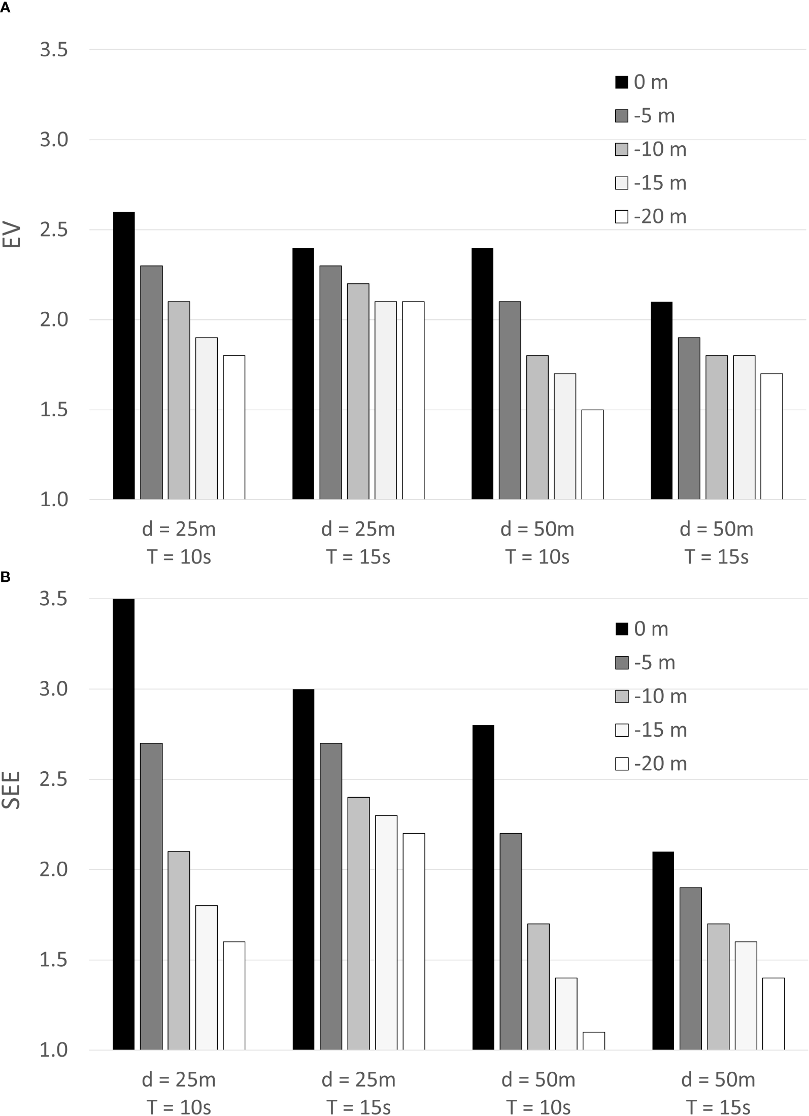
Indices (A) EV and (B) SEE at R1 and R2 related to the position of the farm structure in the water column with ds = 0 m, −5 m, −10 m, −15 m and −20 m, a given wave height of Hs = 5 m and a current speed of Uc = 0.75 m·s−1 for two different wave periods Tp = 10 s and Tp = 15 s and water depths of d = 25 m and 50 m, respectively. The bars show the reduction of the index value in % in relation to the water surface ds = 0 m and the % deviation between the different depths ds.
3 Results
Selected existing aquaculture sites in exposed water bodies that were operational as of April 2024 will be assessed regarding indices developed in Lojek et al. (in review)1 and the actions and changes that have been instituted to extend from sheltered waters to their more exposed locations.
3.1 The application and assessment of the indices in exposed aquaculture farms
All aquaculture requires some “energy” such as water flow to ensure the delivery of oxygen and/or nutrients and/or plankton. In addition, for both, extractive and non-extractive organisms, the dispersal of food remains, faeces and pseudo faeces rely on wave and current energy (Fujita and Goldman, 1985; Gaylord et al., 1994; Larned and Atkinson, 1997; Campbell et al., 2019). Flow also ensures enough oxygen-rich, fresh (clean) and colder water, which mixes and provides cooling during long warm periods, and is therefore an important aspect for many aquaculture candidates (Beveridge, 2008). When using IMTA-based concepts, a minimum movement of the water column is mandatory (Buck and Grote, 2018) for seaweed and organism cultivation to be successful.
As can be seen from the index variations of SEE and EV in Figures 4–7, water depth will also have a significant influence on the species and the aquaculture structural parameters to cultivate at a site. For seaweeds, which generally utilise the surface waters to maximize the sunlight exposure, (except species which are grown deeper such as Macrocystis sp., Laminaria hyperborea, etc.) (Lüning, 1990), the depth of a site is not as important from an operational point of view. However, surface and shallow waters generally have greater wave action and energy than deeper in the water column, therefore the structures need to be more robust. For bivalves such as mussels, there are systems that can tolerate the energy at shallow locations e.g., longtube and longline systems (Buck and Langan, 2017; Goseberg et al., 2017; Newell et al., 2021). The New Zealand longline system has a double backbone with dropper lines which would not be tolerant of shallow, high-energy areas because in order to be viable longer droppers or collectors are required to extend down from the backbone into the water column utilising the available water space efficiently (Newell et al., 2021). Surface finfish systems require depth to accommodate the pen nets as well as free clearance below the pen bottom to disperse effluent. In contrast to floating systems submersible pens require greater depth to accommodate free clearance above the pen for energy dissipation.
In this instance the index can play an illuminating role. A minimum water movement, through a combination of wave and current, is required for a particular species to prosper. Knowing the species minimum requirements and the site’s parameters, it is possible to determine the suitability of the site location in terms of the proposed activities. If the index (amount of energy) is below a minimum, the aquaculture species will not prosper and thus will have a clear detrimental effect on the local ecosystem (Loucks et al., 2012). The carrying capacity of intensive farming systems is directly related to water turnover. In turn, a high index at a given location may indicate the “maximum energy” that is beyond the structural capabilities designed for a particular species or indeed may indicate energy that exceeds the species tolerance. Seaweed and/or bivalves could be detached from the cultivation substrate and lost. Filter feeding of the bivalves can be reduced or even stopped to avoid damage of the filtration apparatus. Seaweed may not be able to uptake nutrients at a certain maximum energy. It could cause stress to the fish in a pen, which could be pushed against the nets, or the nets themselves could reduce their volume because of their enormously large projected area facing tidal currents (Lader and Fredheim, 2006; Fredriksson et al., 2014). This could result in loss of production, poor fish health, structural damage and increased maintenance. These sites are commonly defined as an unfavourable aquaculture site in the context of previously conducted site selection criteria surveys.
In addition to the health and survival of fish and all other extractive species, the technologies used for aquaculture must withstand the demands of sites with higher energy potential. Often the system design as well as the mooring of these high energy sites are different than those in more sheltered areas. In the following, we will analyse the main differences between farms in exposed areas and those in sheltered environments.
3.2 Mussels
Of all the bivalves being considered for cultivation in exposed environments, mussels (e.g. Mytilus edulis, M. galloprovincialis, Perna canaliculus) are becoming the forerunners of the options in terms of production. Mussels, being low value, must be produced in volume to enable a viable enterprise. To produce such volumes at exposed sites, requires large structures that are robust, relatively inexpensive, easy to maintain and operate, and most importantly support the survival, growth and conditioning of the cultivated species. Mussels are usually grown in suspended cultures where the crop hang from substrates on ropes, nets or in baskets, trays or other structures within the water column.
The SEE and EV indices have been applied to a selection of four commercial and semi commercial mussel farms (FS1, FS2, FS3, FS4; Table 3) located in exposed areas in the southern and norther hemispheres (northern hemisphere FS1, FS2, southern hemisphere FS3, FS4). The mean and maximum values (d, Uc, Hs and corresponding Tp) are known for these farms so that they can be assessed using the two indices. In this instance only the maxima 50-year indices will be shown. Since all existing farms are submerged below the water surface (between ds = −3m and ds = −12m), we have also calculated the indices for a hypothetical surface farm at the same locations to illustrate how the energy content at the surface compares to the actual farm position at depth. In Table 3 the four sites, FS1 to FS4 were tested with the primary variation being the water depth (d) of the sites and the position of the farm in the water column (ds). While FS1, FS3 and FS4 are fully functional, FS2 is still in its early stages of development and experiencing several challenges.
Table 3
| Mussel farm sites | d [m] |
Max Hs [m] |
Tp at max Hs [s] |
ds [m] |
Max Uc [m·s−1) |
EV Index |
SEE Index |
|---|---|---|---|---|---|---|---|
| FS1 Lyme Bay, Devon, UK |
28 | 8 | 12 | 0 | 0.5 | 3.2 | 5.2 |
| −5 | 2.9 | 4.2 | |||||
| % deviation from surface index value → |
9.4% | 19.23% | |||||
| FS2 Helgoland, North Sea, Germany |
28 | 9.7 | 13.1 | 0 | 0.93 | 4.2 | 8.6 |
| −12 | 3.5 | 6.0 | |||||
| % deviation from surface index value → |
16.7% | 30.23% | |||||
| FS3 North Island, New Zealand |
45 | 7.6 | 15.2 | 0 | 0.6 | 2.6 | 3.5 |
| −9 | 2.4 | 2.8 | |||||
| % deviation from surface index value → |
7.7% | 20.00% | |||||
| FS4 South Island, New Zealand |
22 | 7.6 | 15.2 | 0 | 0.6 | 3.3 | 5.3 |
| −3 | 3.1 | 4.9 | |||||
| % deviation from surface index value → |
6.1% | 7.6% | |||||
Extreme site and farm parameters of four commercial and semi-commercial mussel farms in exposed waters at two operation depths.
d = mean water depth, Hs = maximum wave height, Tp = wave period of maximum wave height, Uc = maximum current speed, ds = depth of farm structure below surface.Arrow (→) indicates where to find the % deviation from surface index value.
FS1 has its backbone in a submerged configuration of −5 m in the water column, which leads to a reduction of the energy potential of almost 10% for the EV and even up to 20% for the SEE. For FS2 it is as much as approx. 17% (EV) and over 30% (SEE), for FS3 7.7% (EV) and as much as 20% (SEE), and finally 6.1% (EV) and 7.6% (SEE) for FS4, respectively (Table 3). It is evident that lowering a farm in the water column can lead to a reduction in energy. The reduction in energy is limited in the case of FS3 because the farm has a greater water depth (d). For FS4, the percent difference is also less than for FS1 and FS2 despite the similar water depth since there is only a slight reduction below the water surface (ds). To illustrate this energy reduction, the % differences in the respective depths of the four farms FS1–FS4 are shown in the bar chart (Figures 6A, B). FS2 shows the greatest energy reduction, which is due to the worst-case data of this farm with a wave height of HS = 9.3 m and a current speed of Uc = 0.90 m·s−1.
Figure 6
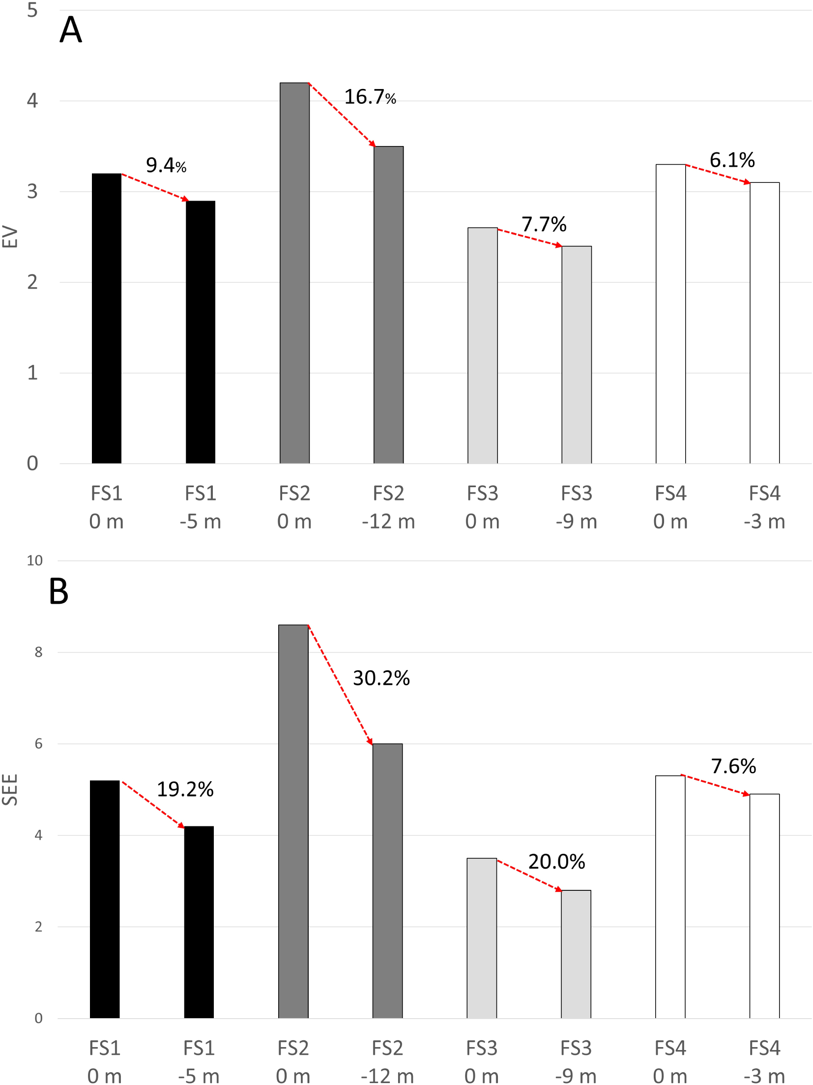
Effects of mussel farm positions within the water column at the water surface and up to −12 m below for farms FS1–FS4 using the (A) EV and (B) SEE indices.
3.3 Seaweed (macroalgae)
Except for a few species that have a high-value (bioactive) component (Holdt and Kraan, 2011), seaweed (e.g. Macrocystis spp., Lessonia app., Ecklonia spp., Undaria spp., Laminaria spp., Saccharina spp) have a low value and can only be grown in large mass cultures to be economically viable. Similar to the cultivation of mussels, large-scale culture facilities, usually in the form of horizontal backbones, grid, ring or raft structures (see Buck and Buchholz, 2004; Tullberg et al., 2022, Lian et al., 2024; Heasman et al. in review4), must be installed to provide substrate for the young plants to reach market size. Like all technologies in exposed areas, the materials used must be durable, robust and inherently stable in order to successfully grow the seaweed on site.
Most seaweed farms worldwide tend to be located in sheltered areas close to the coast, as is the case of China, Indonesia, South Korea, Philippines and other Asian countries (FAO, 2022). Production in the coastal waters of North and South America, Europe and Africa, and the South Pacific (including Australia, New Zealand) is marginal compared to Asia. Whilst many scientific research projects are working on the possibility of open ocean macroalgal farming (Moscicki et al., 2024, Buck et al., 2017), only a few producers have ventured into exposed waters. In Table 4 we have listed one commercial farm (FS5) and three semi-commercial or scientific farms (FS6–FS8). The mean and maximum values of these farm examples are known (d, Uc, Hs and corresponding Tp) and are evaluated using the two indices EV and SEE. As in Table 3, only the maximum indices are shown here, and these data are compared to structures floating at the surface with ds = 0 m as well as in their current original position.
Table 4
| Seaweed farm sites | d [m] |
Max Hs [m] |
Tp at max Hs [s] |
ds [m] |
Max Uc [m∙s−1] |
EV Index |
SEE Index |
| FS5 Funningsfjordur, Faroe Islands, Denmark |
71 | 5.0 | 4.0 | 0 | 0.3 | 2.6 | 3.5 |
| −1 | 2.5 | 3.1 | |||||
| % deviation from surface index value → |
3.9% | 11.4% | |||||
| FS6 Roter Sand, North Sea, Germany |
14 | 6.6 | 12.0 | 0 | 1.5 | 3.9 | 7.6 |
| −2 | 3.7 | 7.0 | |||||
| % deviation from surface index value → |
5.1% | 7.9% | |||||
| FS7 Helgoland, North Sea, Germany |
28 | 9.7 | 13.1 | 0 | 0.93 | 4.2 | 8.6 |
| −5 | 3.8 | 7.3 | |||||
| % deviation from surface index value → |
9.5% | 15.1% | |||||
| FS8 Saco Bay, Maine, US |
50 | 5.3 | 11.4 | 0 | 0.75 | 2.3 | 2.7 |
| −2 | 2.2 | 2.5 | |||||
| % deviation from surface index value → |
4.4% | 7.1% | |||||
Extreme site and farm parameters of four commercial and semi-commercial seaweed farms in exposed waters at two operation depths.
d = mean water depth, Hs = maximum wave height, Tp = wave period of maximum wave height, Uc = maximum current speed, ds = depth of farm structure below surface.Arrow (→) indicates where to find the % deviation from surface index value.
FS5 has its backbone in a submerged configuration at only −1 m in the water column, which results in a small reduction in energy potential of 3.9% for the EV and as much as 11.4% for the SEE. For FS6 the values are also lower, namely 5.1% (EV) and 7.9% (SEE), but for FS7 they are 9.5% (EV) and even 15.1% (SEE) and finally only 4.4%% (EV) and 7.1% (SEE) for FS8 (Table 4), respectively. The lowering of the farm structure results in a lower index (EV and SEE). However, the reduction of the energy potential is lower than in comparison to the mussel farms FS1–FS4, since only low submergible depths are permitted as solar radiation is required to realise good photosynthesis rates. Shading by the sediment load (if present) or the absorption of certain wave lengths at depth will reduce algae growth. The high wave regime and the shallow depth make a commercially successful farm difficult, especially at farm FS6. At FS7, the wave height makes aquaculture difficult so, similar to FS6, the site selection criteria for offshore and/or exposed farming with longline technologies are not met. FS5 has a good location and the wave climate at the given depth does not create any major problems. FS8 can also be declared as a good site as shown by the low indexes. Figures 7A, B illustrate this reduced energy, the percent differences in the respective depths of the four farms FS5–FS8. FS7 shows the greatest energy reduction, but the energy potential is still too high for successful farming of seaweed at this site.
Figure 7

Effects of seaweed farm positions within the water column at the water surface and up to −12 m below for farms FS5–FS8 using the (A) EV and (B) SEE indices.
3.4 Marine finfish
Open ocean finfish farms [e.g. Drum sp. (Totoaba macdonaldi), Pacific Red Snapper (Lutjanus peru), Salmon (Salmo salar), Cobia (Rachycentron canadum)] are also benefiting from utilizing submerged structures to reduce the ocean energy experienced by the crop and equipment. However, finfish farms require more engaged husbandry than bivalve or seaweed farms since daily feeding and mortality recovery are required. As such, submergence is just one of several strategies used to manage ocean energy and the surface conditions are still relevant at these farms to determine the feasibility of operations.
Table 5 shows the relevant oceanographic parameters and resulting EV and SEE values for three commercial fish farms and one perspective farm at the surface and the depth at which the grids are installed. The values reflect 50-year return conditions based on extrapolation of shorter-term data collection efforts at the sites (several years in most cases). The depth of the grid is used as the ds term. The tops of the pens are usually near the grid depth when they are in the submerged position, but this can vary based on the farm. Most of the pen volume and the bulk of the fish are below this level so the EV and SEE values reported in Table 5 are slightly higher than what the fish experience and the forces creating drag on the system. Still, using the grid depth for this analysis allows for consistent comparisons between farms and with FS1–8.
Table 5
| Fish farm sites | d [m] |
Max Hs [m] |
Tp at max H [s] | ds [m] |
Max Uc [m·s−1] |
EV Index |
SEE Index |
|---|---|---|---|---|---|---|---|
| FS9 Caribbean coast, Panama |
64 | 5.9 | 11.0 | 0 | 1.6 | 3.3 | 5.5 |
| 15 | 2.7 | 3.5 | |||||
| % deviation from surface index value → |
18.2% | 36.4% | |||||
| FS10 Hawaii, Kona Coast, US |
60 | 5.7 | 9.0 | 0 | 2.1 | 4.1 | 8.4 |
| 15 | 3.1 | 4.7 | |||||
| % deviation from surface index value → |
24.4% | 44.0% | |||||
| FS11 La Paz, Mexico |
43 | 4.2 | 6.5 | 0 | 0.77 | 2.8 | 3.9 |
| 12 | 1.4 | 1.0 | |||||
| % deviation from surface index value → |
50.0% | 74.4% | |||||
| FS12 New Hampshire, Gulf of Maine, US |
58 | 10.0 | 12.0 | 0 | 0.8 | 4.6 | 10.7 |
| 15 | 2.9 | 4.3 | |||||
| % deviation from surface index value → |
37.0% | 59.8% | |||||
Extreme site and farm parameters of four commercial fish farms in exposed waters at two operation depths.
d = mean water depth, Hs = maximum wave height, Tp = wave period of maximum wave height, Uc = maximum current speed, ds = depth of farm structure below surface.Arrow (→) indicates where to find the % deviation from surface index value.
The finfish farm sites are submerged deeper in the water column than mussels or seaweed resulting in more significant reductions in EV and SEE. This is a result of deeper water at the sites and not needing solar irradiance for growth. FS11 enjoys the largest reduction in EV and SEE with index values falling 50 and 74.4% respectively. Managers at FS9, FS10, and FS11 have indicated that the ocean energy at their sites pose significant challenges for operations and equipment survival so submersible capability of the pens and reduction in EV and SEE are likely essential to make these sites viable.
Table 6 shows the same parameters for FS9 but using mean values instead of 50-year return values. This indicates the conditions, EV, and SEE values in which most operations occur. The values are substantially lower than those shown in Table 5 which is expected since these values are not used to evaluate equipment survival in extreme weather events, but rather the ability of a farmer to operate with reasonable ease and safety. Further, many equipment failures are due to high-frequency fatigue cycles, rather than extreme stress, making the EV and SEE values from averages conditions worthy of consideration in many contexts.
Table 6
| Fish farm sites | d [m] |
Max Hs [m] |
Tp at max Hs [s] |
ds [m] |
Max Uc [m·s−1] |
EV Index |
SEE Index |
|---|---|---|---|---|---|---|---|
| FS9 Caribbean coast, Panama |
64 | 1.5 | 8.3 | 0 | 0.15 | 0.7 | 0.3 |
Average site and farm parameters of the FS9 site.
d = water depth, Hs = mean wave height, Tp = wave period of mean wave height, Uc = mean current speed, ds = depth of farm structure below surface.
4 Discussion
The two indices have shown themselves to be able to provide useful insight to potential and existing aquaculture sites. They can also be used to assess the benefits of not only submerging the structures but how deep the submergence should be. Vessel capability and tolerance to conditions can also benefit from the indices.
These insights should not be considered independently however as there are concerns such as water quality (e.g. levels of oxygen) food availability (in the case of non-fed species), nutrients (in the case of seaweeds) that need to be assessed.
4.1 Extractive species: mussels and seaweed
4.1.1 Mussels
At sheltered, low exposure sites, such as those found in fjord bays or other sheltered regions, may have a maximum (storm conditions) index of approximately 1.5 (EV) and approximately 1.8 (SEE) (data taken from known sites within the Marlborough Sounds, New Zealand, as well as sites in Northern Europe, such as Norway, Denmark, and in Germany). At these index levels, access to the farm was possible more than 90% of the time with vessels capable of operating in 1 m swells. The double-header (also called a backbone) rope longline structure (e.g. New Zealand) or single header-rope longline structure (all countries worldwide) is used in these conditions (Newell et al., 2021). As bivalves grow, the amount of flotation is increased by additional buoys to compensate for the increasing mass. However, the way the double-header rope structure reacts to increased energy found on exposed sites means that this system-design has to be reduced to a single-header rope (Figure 8). The header rope is now also submerged to avoid the surface energy with only a few floats on the surface reducing the amount of energy transferred into the whole structure. Sites FS3 and FS4 (EV: 2.4 and 2.8, SEE: 3.1 and 4.9, respectively) use this general configuration (with some company variations).
Figure 8

Diagrammatic set and forget system – next generation submersible backbone under testing. There is a clamp on the vertical moorings that holds the backbone under the surface.
Although the high energy has resulted in spat and seed rope wrapping around the header rope, floats becoming detached and occasional rope failure (Heasman, pers. obs., New Zealand), in general they are tolerant of conditions and can generate profitable quantities of quality products. Some of the issues and structural stress can be mitigated by changing the orientation of the structure to waves and water currents (Heasman et al., in review)4.
The location at FS4 is, however, shallower and modelling indicates that large waves may be steeper resulting in higher energy at the surface, and there is greater lateral water movement in high wave conditions near the seabed (see Figure 2). At this site the header ropes will be deeper to avoid the surface energy. However, if the header is dropped to 10m then the dropper ropes will be very close to the seabed and subject to the lateral energy being developed in that zone (Figure 2). Therefore, the droppers are shortened to have a safe zone between the seabed and the bottom of the production rope. This results in lighter production lines which results in greater movement. A shortened production line will also result in less production per m of header line, reducing viability.
FS1 is a submerged farm structure which, like FS3 and FS4, consists of a single backbone and is held in place by screw anchors on the seabed and buoyancy floats on the surface. However, unlike FS3 and FS4, these are fitted with long cylindrical fenders. These dip deeper into the water column and do not ride the waves up and down. This means that far less energy from the surface waves is transmitted to the farm structure and mussels located below the surface.
FS2 is not a classic backbone, but a structure that resembles the Smart Farm AS (Norway)7 in a modified form. A hollow HDPE-tube with watertight, welded ends floats on the surface of the water instead of the backbone with floats and serves as buoyancy for the entire structure. It is either connected to anchor blocks or suspended from piles driven into the seabed as is operated in Germany and the Netherlands. In the current, modified version, however, the tube is open and contains 5–7 sealed tubular bodies within that run the full length of the tube. These smaller independent tubes are filled with water or air depending on whether the intention is to submerge or float it. It can therefore be operated in a submerged mode experiencing only a little of the wave-generated surface energy. It is evident from the index value reduction of approx. 17% (EV) or approx. 30% (SEE) that the submerged mode is a necessary modification to the classic Smart Farm to enable it to be used for the safe cultivation of mussels at this site.
4.1.2 Seaweed (macroalgae)
The largest advantage of distant and/or exposed locations is the availability of space. Seaweed culture requires large arrays to be economically attractive, particularly with increased operating expenses associated with operating far from shore or in high energy environments. Further, those production systems must be at or near the surface to ensure algae receive sufficient light for growth. There are only a few cultivated species that can be grown in deeper areas of the water column. From a scientific point of view, most experience exists with the species Macrocystis spp., Lessonia app., Ecklonia spp., Undaria spp., Laminaria spp., Saccharina spp. or other kelp species from the Laminareales order. These algae can cope with lower irradiance and the accompanying light wavelength and do not necessarily have to be grown at the water surface (or slightly below). The near-surface system design excludes most other uses for this area. Thus, stakeholder conflicts are to be expected in the realisation of a seaweed farm at exposed but coastal sites. In addition, cultivation of seaweed near the surface in exposed sites subjects the crop to the strongest wave forces and possibly high-water currents which cause mechanical stress to the crop. Seaweeds with a relatively rigid and upright stipe may have disadvantages over those plants that have a flexible stipe. Rigid cauloids can become overloaded and consequently be damaged or even break, leading to the loss of biomass. More flexible cauloids are capable of quickly reorienting and thus becoming aligned with the direction of the current (Buck and Buchholz, 2005). In this regard, it is known that some kelp species can adapt to harsh conditions, as they develop an increased flexibility of the phyllodes compared to plants in sheltered areas and thus do not break off (Millar et al., 2021). It is also known that some seaweed can be pre-stressed during the nursery phase to reduce dislodgement. According to studies by Buck and Buchholz (2005), it is possible that laminarian species can adapt to strong currents by changing their morphology and taking on a streamlined shape. This process can be accelerated by subjecting the kelp to an artificially induced current shortly after sowing on a substrate and before transferring the seeded ropes to the farm site (Buck et al., 2017). To achieve this, ropes were placed on a rotating drum device and gyrated in the water in the seeding tank. In this way, the plants strengthen their holdfasts and do not dislodge so quickly in harsh conditions. Over and above the stress effects on seaweed biology, care should also be taken to stay below a certain index value when looking for suitable farm sites as stress will affect the technology used. Neushul et al. (1992) indicates that a minimal current of 0.5–1.0 cm·s−1 is necessary for various macroalgal species to be able to absorb nutrients from the water column. In the scope of the SEE index, this would mean that a seaweed farm at the water surface would have to fulfil the index 0.5–1, both at a water depth of 25 m and 50 m. The EV index shows the same result at both depths (25 m and 50 m). A maximum limit for a flow is difficult to identify as each species will vary. For Saccharina latissima, maximum values of up to 1.52 m/s have been identified (Buck and Buchholz, 2004, 2005), for Ulva spp. a maximum current speed of 0.45–1.2 m/s are destructive (Hawe and Smith, 1995). Knox and Kilner (1973) report data of up to 1.8 m/s which not only exceeds or severely limits available technology but would make operations and maintenance difficult or impossible. In the case of successful Macrocystis cultivation, data suggests it can be achieved in high water currents however in this instance a maximum value of 0.3–0.6 m/s is used from the known example farms listed in the Table 2. When choosing a site for growing seaweed with reference to maximum current velocities (and no wave height), no significant influence is found using either the SEE (less than 1 at both depths) or the EV index (1.2 at 25 m depth and 1.4 at 50 m depth), respectively. It may be useful to the reader to apply the additional lens provided by Frieder et al., 2022 who created the Macroalgal Cultivation Modelling System (MACMODS) to represent, among other things, changes in cultivated Macrocystis pyrifera within the farm in relation to different parameters such as light, flow and nutrients in regard to time and space.
However, the index becomes all the more important when wave height is included in the calculation. Some seaweed can withstand wave heights up to 4 m without having a negative effect on growth nor on stability. Wave heights of up to 6.4 m have been measured in some Laminaria reefs (Buck and Buchholz, 2005) without the algae breaking off or the cauloids breaking, but this seems to be an exception. Utter and Denny (1996) measured wave heights of up to 9 m, which severely affected the holdfast and lamina stability of Macrocystis pyrifera. Here, the loss decreased strongly with increasing depth. Based on the farms in Table 3, the wave height data ranges between 0.5 m and 1.0 m. This corresponds to an SEE of 0.5 and 1.2 for both depths, 25 m and 50 m, respectively. As soon as the seaweed farm is exposed to strong currents and additionally, severe wave heights, the energy (and therefore the indices) increase, and plants can be damaged (Denny and Gaylord, 2002), dislodged (Buck and Buchholz, 2005) or the “tip loss” can be increased (Kain, 1979). Therefore, when choosing a site for the cultivation of seaweed related to SEE, the index should not be higher than 4–5, or, in the case of EV, not higher than 5.5. If the exposed site is close to the shore, or the water depth is very shallow, the energy at the site is increased through wave interaction with the seabed increasing the risk of sediment resuspension in the water column. This could harm juvenile plants (Watanabe et al., 2016), create an abrasive effect on the entire plant (Araujo et al., 2012; Watanabe et al., 2016), and the sediment load causes light attenuation in the water column reducing the solar irradiance and algal growth (Kavanaugh et al., 2009). However, environmental conditions in nearshore waters can also vary extensively, affecting seaweed growth and the yield of farmed seaweeds (Kerrison et al., 2015; Bruhn et al., 2016).
Growth comparison of sugar kelp cultured on longlines nearshore at a mouth of a river and kelp grown 12 km offshore indicated significant growth differences based upon season, light variation, and nutrient availability (Chambers pers. Obs.). Nearshore, nutrients were available year-round allowing kelp to grow longer into the summer season before kelp health decreased due to warm temperatures and biofouling (Bartsch et al., 2013). Offshore, nutrient availability was reduced with calming seas and less vertical mixing of the water column. As a result, kelp health diminished by late spring.
In discussions on future seaweed cultivation in multi-use settings (combined with e.g., offshore wind farms) it is noted that the nutrient availability at those sites far away from the coast is another key factor to allow seaweed farming. The tendency to position future offshore wind farms further from shore than they currently are (more than 50–100 km) would mean these areas become less attractive for seaweed farming due to lower nutrient concentration (BSH, 2019; van Duren et al., 2019; Paine et al., 2023).
4.2 Marine finfish
As mentioned in Section 3.4, not all net pens for finfish production in exposed environments utilize the submergence strategy. There are three broad categories employed; flexible gravity pens designed to conform to wave motion, rigid megastructures designed to resist wave energy, and submersible pens designed to evade the strongest surface energy (Heasman et al., in review)4. Production in flexible gravity pens does not create any novel problems or concerns although the existing concerns around equipment damage and fish stress from ocean energy are exacerbated. Pens need to be designed to managed the wave and currents and a fish species or strain needs to have the bioenergetic competency to grow at economically competitive rates in stronger currents and with higher turbulence.
There are very few rigid megastructure pens in operation which leaves a data gap in how this pen style interacts with the ocean environment and the biology of fish. Although several farm sites are in operation, data on specific operational or biological challenges are sparse. Salmar Aker Ocean operates the Ocean Farm 1 at a site with 5m significant wave heigh (currents speed not reported) and has completed three grow out cycles as of January 2024 (Romuld, 2024). Without further site data, the SEE and EV indices cannot be calculated.
Submersible systems create some significant differences from the technology used at sheltered sites. Perhaps the most important factor to note is the ability to utilize locations that have been deemed too rough for traditional net pens. The available space to farm fish using systems that can handle rougher environments is well beyond what is needed to meet global seafood demand (Kapetsky et al., 2013; Gentry et al., 2017; although it should be noted that macro-scale analysis like these may not capture economic constraints well). As shown in Table 5, submerging pens and grids 10–15 m below the surface reduces the effective energy level substantially, allowing higher energy locations to be utilized without a commensurate increase in the risk of equipment damage or fish escapes. Similarly, since the drag loads on the system do not increase as much at depth as is observed at the surface, anchors and rope sizes may not need to be increased as much, saving on capital costs relative to a surface-based system at that site. This is important from a global food security standpoint but is most impactful when considering certain regions that do not have sheltered coastlines. Many countries in Central America and Southeast Asia are in hurricane belts so even locations that do have some protection may still be subjected to extreme conditions with some regularity.
Turbulent water can affect fish in a few ways. Barbier et al. (2024) observed a 5% reduction in fish size over an 8-week grow out trial that created turbulent conditions in a tank environment. They observed significant differences in feed intake and behaviour during the first three weeks after which the fish acclimated and performed similarly thereafter. However, at a farm, turbulent conditions are episodic, so acclimation may be inconsistent between sites depending on how sever and frequent turbulent conditions are. Johannessen et al. (2020) has observed salmon avoiding surface waters during turbulent conditions indicating a stress response or less optimal conditions. The Barbier et al. (2024) article concluded that salmon should be able to adapt to turbulent conditions although exposed farms may observe different results depending on the specific site conditions. Submerging pens should alleviate this concern as wave energy is reduced. Studies on other species are not available although species with closed or no swim bladders may be better equipped to avoid surface waters. Likewise, farms with feeding systems that deliver feed below the surface would be expected to reduce exposure of the fish to rough surface waters.
High energy environments have a higher capacity to disperse nutrients and effluent from a fish pen, which can reduce impacts on the local benthic environment (Welch et al., 2019). In cases where fish farms have a high dispersion capacity and oligotrophic water, the stocking density at farms may be able to be increased above what is commonly observe elsewhere while maintaining benthic impacts at tolerable levels. Other limitations on stocking density such as density-related stress and disease risk would still be limiting.
The finfish species being cultured in open ocean environments are similar to what is produced in sheltered waters. Most species benefit from open ocean conditions as more stable temperature and dissolved oxygen are preferrable, as well as reduced connectivity with surface runoff. Stronger currents are also helpful to many species, stimulating growth (Jobling et al., 1993; Brown et al., 2011), reducing stress and aggression (Jobling et al., 1993), and improving flesh quality (Huang et al., 2021). However demersal or reef species often have lower aerobic scope so they may not see a benefit from stronger currents and can struggle in consistently high currents and suffer from the higher energy demand (Bjørnevik et al., 2003). If extreme currents are sustained for long periods, fish can become exhausted and pile up at the bottom and back of the pen creating stress, damage to scales and skin, and mortality.
Salmon is receiving the most interest due to market demand, familiarity with the species, and availability of seedstock. There are concerns around raising salmon in submerged pens since salmonids are physostomal and require access to air to inflate their swim bladders. Researchers are exploring techniques to mitigate this concern (Dempster et al., 2009; Korsøen et al., 2009; Yigit et al., 2024). Several tropical and sub-tropical species are gaining increased attention for open ocean farms since the technology needed to site farms in hurricane or typhoon-prone areas has only recently become available. Cobia, several Seriola species, red snapper, red drum, pompano, and tuna have all received commercial interest or are being actively produced in open ocean farms (Sclodnick, personal experience).
4.3 Vessels and operation and maintenance
Vessels that are being used for exposed mussel and seaweed farming at the farm sites FS1 to FS4 are generally large (>24 m length). The vessel size provides a platform that can tolerate the larger wave conditions ensuring access to the site for a minimum period during the year. This is about being able to maneuver freely within the farm and between the structures (longlines, longtubes etc.; Buck and Grote, 2018). Large vessel can add significant stress to the culture structures while attached to the structures during servicing, seeding or harvesting particularly if the current or wind speeds becomes stronger, or the wave height becomes higher increasing the indices.
The trends in vessel requirements for offshore production of finfish are similar to those for bivalves and seaweed. The distance between the farm and port is typically longer, making it essential that vessels can carry as much feed or harvested fish as possible. Also, the mooring system components (lines, anchors, etc) are subject to more wear and tear and are often larger, requiring more heavy-duty operations vessels. The rough conditions at open ocean sites makes it less feasible to use barges that are permanently station at the farm, requiring vessels to traverse the distance from shore each day, in most cases.
It has been demonstrated that with increasing submergence depth of any farm structure, be they mussels, seaweed or fish, the energy content that can act on the structure is reduced. However, with increasing depth and exposure, work on the farm becomes more complex and difficult. O&M on the structure, the mooring or the crop, such as monitoring, seeding, harvesting, other maintenance types of work or simply returning the structure back from its submerged position to the surface to allow further operation becomes more intricate and difficult. At this time there are three potential solutions to this issue. The first being a structure that is fully floated and is held down by releasable clamps e.g., set and forget (Figure 8) (Heasman et al., in review)4. A second solution could have the ability to be inflated either manually or automatically. The latter is appealing but is potentially complex and has further maintenance considerations. Access to electricity (possibly in wind farms) would greatly simplify some of these problems. This approach should be considered in any potential multi-use scenarios involving offshore wind energy farms (Buck and Langan, 2017; Schupp et al., 2019).
In terms of general structure operation and survival, the indices will provide an indication as to when the components of the structural system need to be improved, bolstered, or submerged. An important consideration for operation and structural survival is the interaction and transfer of energy between the floatation and moorings of a structure. Figures 9A, B shows examples of suggested improvements or changes required to accommodate the mooring/float relationship and variations to increase tolerance of the seas with rising energy. In general, an increase in robustness of mooring and header ropes (where applicable), floats and attachment points are required with increasing energy. In addition, the shape and attachment of floats may change (e.g. from a round to cylinder in shape) or floats may become more complex and include inflatable bladders or multiple inflatable tubes within a larger tube. As the energy increases further, the structure may be submerged to avoid the surface energy. In Figure 9A, examples of how buoyancy and design can be changed to improve durability and robustness with increased exposure. Object 1 is a standard spherical buoy, used in sheltered waters as it rides on the surface due to its shape. Object 2 represents a spar or fender float that can be used with increasing wave action, as it can be pulled down more easily and reducing tension shock events possibilities. Object 3 represents a long-tube design, where the backbone is hollow and thus forms the buoyancy body. Object 4 represent a header rope or long-tube design float that is submerged, fitted with additional small buoyancy buoys at depth and has spar/fenders at the top that only serve as markers. The culture ropes are hung from this unit. Object 5 is a submerged long tube with marker spar/fender floats and internal tubes or bladders where the air pressure can be changed. Object 6 is similar to Object 5, but with no marker to the water surface, and culture structures are suspended from this unit. The illustrations on the right in Figure 9 shows the decrease in the orbital wave (see also Figure 2). The red dashed line designates the photic zone where sufficient light still seeps through so that seaweed can photosynthesise. This can be taken a step further by having the structure completely bottom referenced (i.e. all structural flotation is submerged and maintained in position by direct attachment to the seabed) with only a surface marker, e.g. as seen in the Shellfish Tower (Heasman et al., 2021). Figure 9B show examples of anchoring and mooring for various degree of exposure. Mooring system 1 a, b and c (block, Danforth, screw/helix respectively) single moorings which can be used for lower energy areas. They generally have a narrow arc of attachment to the surface structures, while mooring system 2 involve larger blocks on which more vertical and lateral forces can be exerted without dislodgment. Mooring system 3 represents screw or helix moorings which, with the correct substrate, can be designed for vertical and lateral tensions. There are some limits to these anchors both in deployment depth and tensions applied; while mooring system 4 may be suitable for holding systems in high energy. They are generally a single direction, primarily lateral tensioned system where one anchor supports the next.
Figure 9
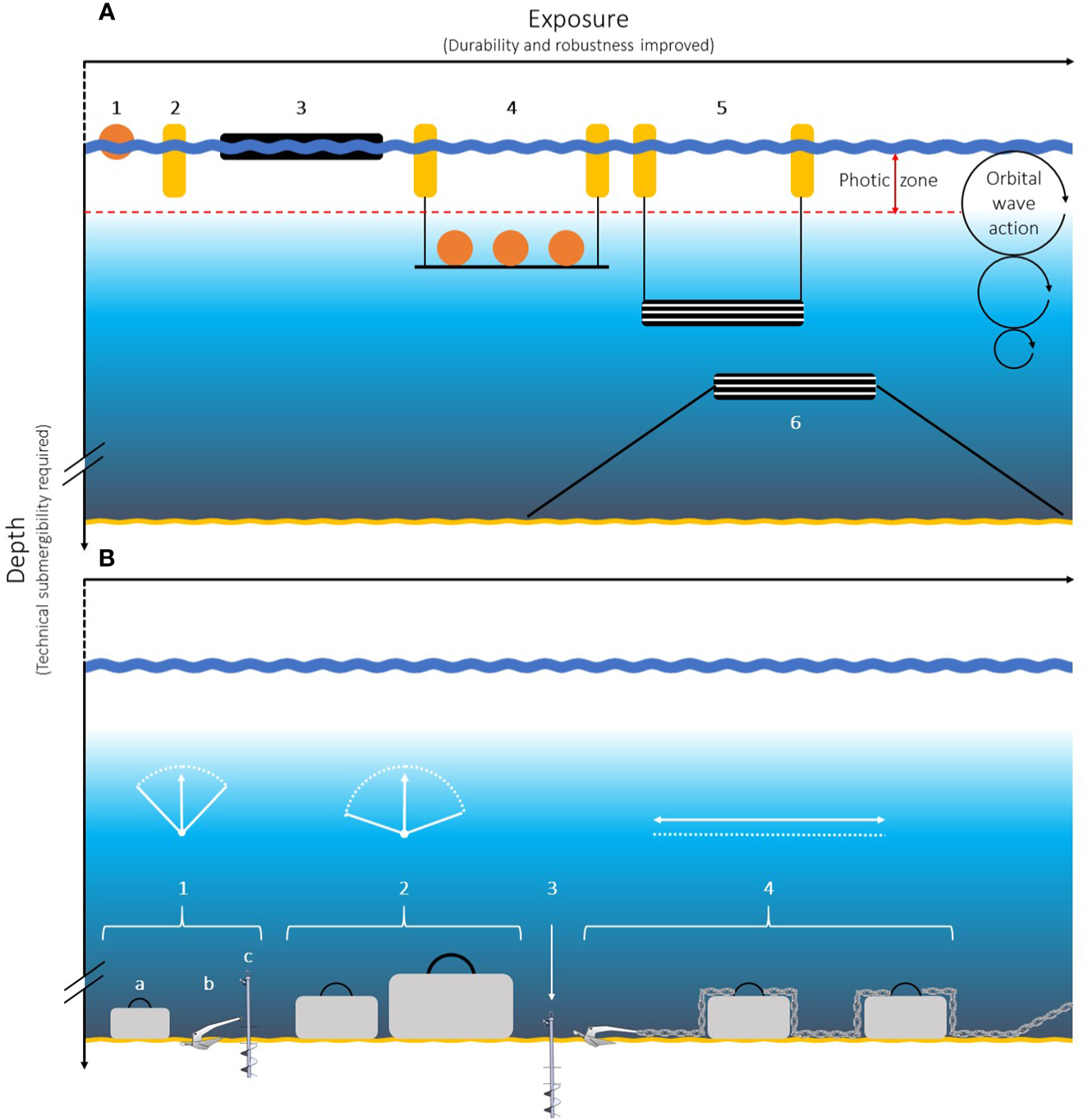
Illustration of primary components of farming systems for the cultivation of extractive organisms (mussels, seaweed). Shown are examples of buoyancy units (A) and moorings (B) of different system designs with increasing exposure.
The increasing complexity associated with rising indices will indicate the need to include or upgrade smarter operational procedures, automation, submergence and a suite of sensors (e.g. wave height, duration and direction, water currents, turbidity). Operational procedures will include improved staff health and safety, increasing robustness of equipment, and tolerance of vessels to operating in larger waves. Semi or full automation will reduce the necessity of direct human involvement and could possibly respond to conditions without human intervention. This intervention may include submergence of the structures to avoid and escape from increasing surface energy. Sensors will be required to facilitate immediate data transfer for any human or automated responses.
4.4 Future needs
There are other potential structures that have either been tested and discarded or are in development for sites of increasing energy (e.g. the Smart Farm concept with a hollow, inflatable long tube or variations of it). Circular designs are possible and stronger in some respects as they distribute energy through the structure, but they are less space-efficient and more difficult to seed, harvest and operate (e.g., the Spanish Medusa shellfish structure or the offshore ring (Buck and Buchholz, 2004). Another disadvantage is the fact that such constructions have a one-point-mooring, which in principle is easy to handle, but in operation will have a certain radius as a watch circle and thus inevitably increases the necessary cultivation area. The linear designs are space-efficient and allow for continuous or “long lines” which are time-efficient for operations and management.
Structures to produce oysters in exposed regions are very limited but some are being tested. Structures suspended from mussel backbones (Heasman et al., in review)4 have been used with success experimentally on FS3 (EV 2.4 or SEE 2.8) but are yet to be tested commercially. The shellfish tower (Heasman et al., 2021) has responded well to the conditions on the same site with ease and is suggested to be able to tolerate considerably higher conditions (EV >7.5 or SEE > 9) providing there is sufficient depth to submerge it below significant wave interaction. This structure is also being tested to produce scallops.
Our data sources utilised in the indices includes our most accurate estimate of the worst-case scenarios, reflecting extreme wave heights and current velocities which may only happen every 50 years. However future assessments may show that the estimations are insufficient since climate change is expected to both increase and decrease significant wave heights, depending on location (Lobeto et al., 2021) and wave form (Lemos et al., 2021; Lobeto et al., 2022). Therefore, vigilance will be required regarding the maintenance and updating of data when using the indices in the future. Catastrophic events such as tidal waves have not been considered however the indices may be used to estimate their potential influence.
5 Conclusions
The indices have shown themselves to be useful tools in the general assessment of the energy that will influence the species and structure selection at potential aquaculture sites. This information can help prospective fish farmers characterize their sites concisely and accurately to consultants, regulators, equipment vendors, and insurance brokers. Using case studies of successful farms in association with the energy indices there can be confidence in the determination of the tolerances of the structures and the ability of them to cultivate their relevant species.
It is important to note that the indices do not provide an indication as to the potential financial success of a site. This requires other inputs relating to structure costs, annual production, distance from port, CapEx, etc. Once the indices have indicated the practicability of the site relative to structural, species and vessel aspects to now add different lenses of assessment to determine the variables that are still open.
In the case of seaweed production in exposed seas the limiting factor is the tolerance of seaweed to energy and as such a maximum index can be described for seaweed production. For bivalves and finfish, the maximum index will be influenced by the structural design, position in the water column, orientation (for linear systems), species, depth, O&M and vessel access.
The indices will provide some indication of vessel size requirements, but its operational parameters will vary according to the species, structures it is supporting, its purpose within the husbandry/harvesting/maintenance process and the distances it has to travel.
Orientation of linear structures is important for the reduction of damage and maintenance and potential loss of crop.
Shallow waters in exposed conditions increase energy and the associated structure and husbandry requirements.
Statements
Data availability statement
The raw data supporting the conclusions of this article will be made available by the authors, without undue reservation.
Author contributions
KH: Conceptualization, Funding acquisition, Investigation, Methodology, Project administration, Writing – original draft, Writing – review & editing. TS: Conceptualization, Methodology, Writing – original draft, Writing – review & editing. NG: Methodology, Writing – original draft, Writing – review & editing. NS: Visualization, Writing – original draft, Writing – review & editing. MC: Writing – original draft, Writing – review & editing. TD: Methodology, Validation, Writing – original draft, Writing – review & editing. SR: Validation, Visualization, Writing – original draft, Writing – review & editing. HF: Writing – original draft, Writing – review & editing. BB: Conceptualization, Investigation, Methodology, Validation, Visualization, Writing – original draft, Writing – review & editing.
Funding
The author(s) declare financial support was received for the research, authorship, and/or publication of this article. This manuscript was partially supported by the Ministry of Business, Innovation and Employment, New Zealand (CAWX2102).
Conflict of interest
Authors TD and SR were employed by the company Kelson Marine Co. Author TS was employed by the company Innovasea.
The remaining authors declare that the research was conducted in the absence of any commercial or financial relationships that could be construed as a potential conflict of interest.
Publisher’s note
All claims expressed in this article are solely those of the authors and do not necessarily represent those of their affiliated organizations, or those of the publisher, the editors and the reviewers. Any product that may be evaluated in this article, or claim that may be made by its manufacturer, is not guaranteed or endorsed by the publisher.
Supplementary material
The Supplementary Material for this article can be found online at: https://www.frontiersin.org/articles/10.3389/faquc.2024.1427168/full#supplementary-material
Footnotes
1.^Lojek, O., Goseberg, N., Fore, H.M., Dewhurst, T., Bölker, T., Heasman, K.G., et al. Hydrodynamic exposure – on the quest to deriving quantitative metrics for mariculture sites.
2.^Sclodnick, T., Chambers, M., Costa-Pierce, B.A., Dewhurst, T., Goseberg, N., Heasman, K.G., et al. From “open ocean” to “exposed aquaculture”: why and how we are changing the standard terminology describing “offshore aquaculture”.
3.^Dewhurst, T., Richerich, S., MacNicoll, M., Baker, N., and Moscicki, Z. The effect of site exposure index on the required structural capacities costs of aquaculture structures.
4.^Heasman, K.G., Scott, N., Sclodnick, T., Chambers. M., Costa-Pierce, B., Dewhurst, T., et al. Variations of aquaculture structures, operations, and maintenance with increasing ocean energy.
5.^Markus, T. Finding the right spot: laws promoting sustainable siting of open ocean aquaculture activities.
References
1
Ahmed N. Thompson S. Glaser M. (2019). Global aquaculture productivity, environmental sustainability, and climate change adaptability. Environ. Manage.63, 159–172. doi: 10.1007/s00267-018-1117-3
2
Araujo R. Arenas F. Åberg P. Sousa-Pinto I. Serrão E. A. (2012). The role of disturbance in differential regulation of co-occurring brown algae species: Interactive effects of sediment deposition, abrasion and grazing on algae recruits. J. Exp. Mar. Biol. Ecol.422–423, 1–8. doi: 10.1016/j.jembe.2012.04.006
3
Atalah J. Fletcher L. M. Hopkins G. A. Heasman K. Woods C. M. C. Forrest B. M. (2016). Preliminary assessment of biofouling on offshore mussel farms. J. World Aquaculture Soc.43, (3) 376–386. doi: 10.1111/jwas.12279
4
Barbier E. Oppedal F. Hvas M. (2024). Atlantic salmon in chronic turbulence: Effects on growth, behaviour, welfare, and stress. Aquaculture.582, 740550. doi: 10.1016/j.aquaculture.2024.740550
5
Bartsch I. Vogt. J. Pehlke C. Hanelt D. (2013). Prevailing sea surface temperatures inhibit summer reproduction of the kelp Laminaria digitata at Helgoland (North Sea). J. Phycology49, 1061–1073. doi: 10.1111/jpy.12125
6
Beveridge M. C. (2008). Cage aquaculture (Oxford: Blackwell Publishing).
7
Bjørnevik M. Karlsen Ø. Johnson I. A. Kiessling A. (2003). Effect of sustained exercise on white muscle structure and flesh quality in farmed cod (Gadus morhua L.). Aquaculture Res.34, 55–64. doi: 10.1046/j.1365-2109.2003.00794.x
8
Brown E. J. Bruce M. Pether S. Herbert N. A. (2011). Do swimming fish always grow fast? Investigating the magnitude and physiological basis of exercise-induced growth in juvenile New Zealand yellowtail kingfish, Seriola lalandi. Fish Physiol. Biochem.37, 327–336. doi: 10.1007/s10695-011-9500-5
9
Bruhn A. Tørring T. B. Thomsen M. Canal-Vergés P. Nielsen M. M. Rasmussen M. B. et al . (2016). Impact of environmental conditions on biomass yield, quality, and bio-mitigation capacity of Saccharina latissima. Aquaculture Environ. Interact.8, 619–636. doi: 10.3354/aei00200
10
BSH (2019). Area development plan 2019 for the German North and Baltic Seas (Flächenentwicklungsplan 2019 für die deutsche Nord- und Ostsee). Federal Maritime Hydrographic Agency (Bundesamt für Seeschifffahrt und Hydrographie - BSH)7608, 202.
11
Buck B. H. Buchholz C. M. (2004). The Offshore-Ring: A new system design for the open ocean aquaculture of macroalgae. J. Appl. Phycology16, 355–368. doi: 10.1023/B:JAPH.0000047947.96231.ea
12
Buck B. H. Bjelland H. V. Bockus A. Chambers M. Costa-Pierce B. A. Dewhurst T. et al (2024). Resolving the term “offshore aquaculture” by decoupling “exposed” and “distance from the coast”. Front. Aquac.3, 14280562. doi: 10.3389/faquc.2024.14280562
13
Buck B. H. Buchholz C. M. (2005). Response of offshore cultivated Laminaria saccharina to hydrodynamic forcing in the North Sea. Aquaculture250, 674–691. doi: 10.1016/j.aquaculture.2005.04.062
14
Buck B. H. Grote B. (2018). “Seaweed in high energy environments: protocol to move saccharina cultivation offshore,” in Protocols for macroalgae research. Eds. CharrierB.WichardT.ReddyC. R. K. (Boca Raton: CRC Press, Taylor & Francis Group). doi: 10.1201/b21460
15
Buck B. H. Langan R. (2017). “Aquaculture perspective of multi-use sites in the open ocean,” in The untapped potential for marine resources in the anthropocene. Eds. BelaB. H.RichardL. (Springer, Cham), 404. doi: 10.1007/978-3-319-51159-7
16
Buck B. H. Nevejan N. Wille M. Chambers M. Chopin T. (2017). “Offshore and multi-use aquaculture with extractive species: seaweeds and bivalves,” in Aquaculture perspective of multi-use sites in the open ocean: The untapped potential for marine resources in the Anthropocene. Eds. BuckB. H.LanganR. (Switzerland: Springer), 23–69.
17
Campbell I. Macleod A. Sahlmann C. Neves L. Funderud J. Øverland M. et al . (2019). The environmental risks associated with the development of seaweed farming in europe - prioritizing key knowledge gaps. Front. Mar. Sci.6. doi: 10.3389/fmars.2019.00107
18
Dean R. G. Dalrymple R. A. (1991). Water wave mechanics for engineers and scientists (Advanced series on ocean engineering: vol. 2) (Singapore: World Scientific). doi: 10.1142/ASOE
19
Dempster T. Korsøen Ø. Folkedal O. Juel J. Oppedal F. (2009). Submergence of Atlantic salmon (Salmo salar L.) in commercial scale sea-cages: A potential short-term solution to poor surface conditions. Aquaculture.288, 254–263. doi: 10.1016/j.aquaculture.2008.12.003
20
Denny M. Gaylord B. (2002). The mechanics of wave-swept algae. J. Exp. Biol.205, 1355–1362. doi: 10.1242/jeb.205.10.1355
21
FAO (2022). The state of world fisheries and aquaculture 2022. Towards blue transformation (Rome: Food and Agriculture Organisation of the United Nations (FAO). doi: 10.4060/cc0461en
22
Fredriksson D. W. DeCew J. Lader P. Volent Z. Jensen Ø. Willumsen F. V. (2014). A finite element modeling technique for an aquaculture net with laboratory measurement comparisons. Ocean Eng.83, 99–110. doi: 10.1016/j.oceaneng.2014.03.005
23
Frieder C. A. Yan C. Chamecki M. Dauhajre D. McWilliams J. C. Infante J. et al . (2022). A macroalgal cultivation modeling system (MACMODS): evaluating the role of physical-biological coupling on nutrients and farm yield. Front. Mar. Sci.9. doi: 10.3389/fmars.2022.752951
24
Froehlich H. E. Smith A. Gentry R. R. Halpern B. S. (2017). Offshore aquaculture: I know it when I see it. Front. Mar. Sci.4, 154. doi: 10.3389/fmars.2017.00154
25
Fujita R. M. Goldman J. C. (1985). Nutrient flux and growth of the red alga Gracilaria tikvahiae McLachlan (Rhodophyta). Bot. Mar.28, 265–268. doi: 10.1515/botm.1985.28.6.265
26
Galparsoro I. Murillas A. Pinarbasi K. Sequeira A. M. M. Stelzenmüller V. Borja Á. et al . (2020). Global stakeholder vision for ecosystem-based marine aquaculture expansion from coastal to offshore areas. Rev. Aquacult.12, 2061–2079. doi: 10.1111/raq.12422
27
Gaylord B. Blanchette C. A. Denny M. W. (1994). Mechanical consequences of size in wave-swept algae. Ecol. Monogr.64, 287–313. doi: 10.2307/2937164
28
Gentry R. R. Froehlich H. E. Grimm D. Kareiva P. Parke M. Rust M. et al . (2017). Mapping the global potential for marine aquaculture. Nat. Ecol. Evolution.1, 1317–1324. doi: 10.1038/s41559-017-0257-9
29
Gieschen R. Schwartpaul C. Landmann J. Fröhling L. Hildebrandt A. Goseberg N. (2020). Large-scale laboratory experiments on mussel dropper lines in ocean surface waves. J. Mar. Sci. Eng.9, 29. doi: 10.3390/jmse9010029
30
Goseberg N. Chambers M. D. Heasman K. Fredriksson D. Fredheim A. Schlurmann T. (2017). Technological approaches to longline-and cage-based aquaculture in open ocean environments pp. (71–95). In: Buck and Langan (Eds), Aquaculture Perspective of Multi-Use Sites in the Open Ocean: The Untapped Potential for Marine Resources in the Anthropocene. Springer International Publishing. doi: 10.1007/978-3-319-51159-7_3
31
Hawe I. Smith R. (1995). Effect of current velocity on the detachment of thalli of Ulca lactuca (Chlorophyta) in a New Zealand estuary. J. Phycol.31, 875–880. doi: 10.1111/j.0022-3646.1995.00875.x
32
Heasman K. G. Scott N. Smeaton M. Goseberg N. Hildebrandt A. Vitasovich P. et al . (2021). New system design for the cultivation of extractive species at exposed sites - Part 1: System design, deployment and first response to high-energy environments. J. Appl. Mar. Science Vol110, 102603. doi: 10.1016/j.apor.2021.102603
33
Holdt S. L. Kraan S. (2011). Bioactive compounds in seaweed: functional food applications and legislation. J. Appl. Phycology23, 543–597. doi: 10.1007/s10811-010-9632-5
34
Huang X. Hegazy A. M. Zhang X. (2021). Swimming exercise as potential measure to improve flesh quality of cultivable fish: A review. Aquaculture Res.52, 5978–5989. doi: 10.1111/are.15510
35
Jobling M. Baardvik B. M. Christiansen J. S. Jørgensen E. H. (1993). The effects of prolonged exercise training on growth performance and production parameters in fish. Aquaculture Int.1, 95–111. doi: 10.1007/BF00692614
36
Johannessen Á. Patursson Ø. Kristmundsson J. Dam S. P. Klebert P. (2020). How caged salmon respond to waves depends on time of day and currents. PeerJ8, e9313. doi: 10.7717/peerj.9313
37
Kain J. M. (1979). A view of the genus Laminaria. Annu. Rev. Oceanogr. Mar. Biol.17, 101–161.
38
Kapetsky J. M. Aguilar-Manjarrez J. Jenness J. (2013). A global assessment of offshore mariculture potential from a spatial perspective (Rome: FAO Fisheries and Aquaculture Technical Paper 549).
39
Kavanaugh M. T. Nielsen K. J. Chan F. T. Menge B. A. Letelier R. M. Goodrich L. M. (2009). Experimental assessment of the effects of shade on an intertidal kelp: Do phytoplankton blooms inhibit growth of open coast macroalgae? Limnology Oceanography54, 276–288. doi: 10.4319/lo.2009.54.1.0276
40
Kerrison P. D. Stanley M. S. Edwards M. D. Black K. D. Hughes A. D. (2015). The cultivation of European kelp for bioenergy: Site and species selection. Biomass Bioenergy80, 229–242. doi: 10.1016/j.biombioe.2015.04.035
41
Knox G. A. Kilner A. R. (1973). “The ecology of the avon-heathcote estuary,” (Estuarine Research Unit: University of Canterbury), 358.
42
Korsøen Ø.J. Dempster T. Fjelldal P. G. Oppedal F. Kristiansen T. S. (2009). Long-term culture of Atlantic salmon (Salmo salar L.) in submerged cages during winter affects behaviour, growth and condition. Aquaculture.296, 373–381. doi: 10.1016/j.aquaculture.2009.08.036
43
Lader P. F. Fredheim A. (2006). Dynamic properties of a flexible net sheet in waves and current—A numerical approach. Aquacultural Eng.35, 228–238. doi: 10.1016/j.aquaeng.2006.02.002
44
Landmann J. Fröhling L. Gieschen R. Buck B. H. Heasman K. Scott N. et al . (2021). Drag and inertia coefficients of live and surrogate shellfish dropper lines under steady and oscillatory flow. Ocean Eng.235, 109377. doi: 10.1016/j.oceaneng.2021.109377
45
Larned S. T. Atkinson M. J. (1997). Effects of water velocity on NH4 and PO 4 uptake and nutrient-limited growth in the macroalga Dictyosphaeria cavernosa. Mar. Ecol. Prog. Ser.157, 295–302. doi: 10.3354/meps157295
46
Lemos G. Semedo A. Hemer M. Menendez M. Miranda P. M. A. (2021). Remote climate change propagation across the oceans — the directional swell signature. Environ. Res. Lett.16, 064080. doi: 10.1088/1748-9326/ac046b
47
Lian Y. Boamah S. O. Pan Z. Zheng J. Chen W. Ma G. et al . (2024). Engineering design and economic analysis of offshore seaweed farm. Front. Mar. Sci.11. doi: 10.3389/fmars.2024.1276552
48
Lobeto H. Menendez M. Losada I. J. (2021). Future behavior of wind wave extremes due to climate change. Sci. Rep.11, 7869. doi: 10.1038/s41598-021-86524-4
49
Lobeto H. Menendez M. Losada I. J. Hemer M. (2022). The effect of climate change on wind-wave directional spectra. Global and Planetary change213, 103820. doi: 10.1016/j.gloplacha.2022.103820
50
Loucks R. H. Smith R. E. Fisher C. V. Fisher E. B. (2012). Copper in the sediment and sea surface microlayer near a fallowed, open-net fish farm. Mar. pollut. Bull.64, 1970–1973. doi: 10.1016/j.marpolbul.2012.05.025
51
Lüning K. (1990). Seaweeds: their environment, biogeography, and ecophysiology (New York: John Wiley & Sons), 544.
52
Millar R. Houghton. J. D. R. Kregting L. (2021). The stress and strain of life – how differences in the mechanical properties and cellular composition enable the kelp Laminaria digitata to thrive in different hydrodynamic environments. Mar. Env. Res.169, 105330. doi: 10.1016/j.marenvres.2021.105330
53
Morro B. Davidson K. Adams T. P. Falconer L. Holloway M. Dale A. et al . (2021). Offshore aquaculture of finfish: Big expectations at sea. Rev. Aquaculture14, 791–815. doi: 10.1111/raq.12625
54
Moscicki Z. Swift M. R. Dewhurst T. MacNicoll M. Chambers M. Tsukrov I. et al . (2024). Design, deployment, and operation of an experimental offshore seaweed cultivation structure. Aquacultural Eng. 305. doi: 10.1016/j.aquaeng.2024.102413
55
Neushul M. Benson J. Harger B. W. W. Charters A. C. (1992). Macroalgal farming in the sea: water motion and nitrate uptake. J. Appl. Phycology4, 255–265. doi: 10.1007/BF02161211
56
Newell C. Heasman K. G. Smaal A. Jiang Z. (2021). Mussel aquaculture. Ed. ShumwayS. (5M books, Essex, UK: Molluscan Shellfish Aquaculture: A Practical Guide, 5m Publishing), 552.
57
Olsen Y. Otterstad O. Duarte C. M. (2008). Status and future perspectives of marine aquaculture. Aquaculture Ecosystem, 293–319. In: HolmerM.BlackK.DuarteC. M.MarbàN.KarakassisI. (Eds.). (2007). Aquaculture in the Ecosystem. Springer Science & Business Media. 314pp.
58
Paine E. R. Boyd P. W. Strzepek R. F. Ellwood M. Brewer E. A. Diaz-Pulido G. et al . (2023). Iron limitation of kelp growth may prevent ocean afforestation. Commun. Biol.6, 607. doi: 10.1038/s42003-023-04962-4
59
Painter S. C. Lapworth D. J. Woodward E. M. S. Kroeger S. Evans C. D. Mayor D. J. et al . (2018). Terrestrial dissolved organic matter distribution in the North Sea. Sci. Total Environ.630, 630–647. doi: 10.1016/j.scitotenv.2018.02.237
60
Rodriguez-Rodrıguez D. Rees S. E. Rodwell L. D. Attrill M. J. (2015). Assessing the socioeconomic effects of multiple-use MPAs in a European setting: A national stakeholders’ perspective. Environ. Sci. Policy48, 115–127. doi: 10.1016/j.envsci.2014.12.020
61
Romuld T. S. (2024). SalMar Aker Ocean – Status and current strategic focus (Bergen, Norway: North Atlantic Seafood Forum).
62
Schupp M. F. Bocci M. Depellegrin D. Kafas A. Kyriazi Z. Lukic I. et al . (2019). Toward a common understanding of ocean multi-use. Front. Mar. Sci.6, 165. doi: 10.3389/fmars.2019.00165
63
Tullberg R. M. Nguyen H. P. Wang C. M. (2022). Review of the status and developments in seaweed farming infrastructure. J. Mar. Sci. Eng.10, 1447. doi: 10.3390/jmse10101447
64
Utter B. D. Denny M. W. (1996). Wave-Induced forces on the giant kelp macrocystis pyrifera (Agardh): field test of a computational model. J. Exp. Biol.199, 2645–2654. doi: 10.1242/jeb.199.12.2645
65
van Duren L. Jansen H. Timmermans K. (2019). Eenrealistische kijk op zeewierproductie in de Noordzee. (Wageningen, Netherlands) 11, Project report No. BO-43-023.03-005, reference No. 1930336-MP-LvdB-lcs.
66
Visch W. Nylund G. M. Pavia H. (2020). Growth and biofouling in kelp aquaculture (Saccharina latissima): the effect of location and wave exposure. J. Appl. Phycology32, 3199–3209. doi: 10.1007/s10811-020-02201-5
67
Watanabe H. Ito M. Matsumoto A. Arakawa H. (2016). Effects of sediment influx on the settlement and survival of canopy-forming macrophytes. Sci. Rep.6, 18677. doi: 10.1038/srep18677
68
Welch A. Knapp A. El Tourky S. Daughtery Z. Hitchcock G. Benetti D. (2019). The nutrient footprint of a submerged-cage offshore aquaculture facility located in the tropical Caribbean. J. World Aquaculture Society.50, 299–316. doi: 10.1111/jwas.12593
69
Yigit Ü. Yigit M. Ergün S. Kusku H. Ek H. Maita M. (2024). Analysis of the economic performance of salmon farming in submerged and surface cages in the Black Sea. Aquaculture Int.32, 101–118. doi: 10.1007/s10499-023-01155-y
Summary
Keywords
mussels, seaweed, exposed aquaculture, energy index, site selection, marine finfish
Citation
Heasman KG, Sclodnick T, Goseberg N, Scott N, Chambers M, Dewhurst T, Rickerich S, Føre HM and Buck BH (2024) Utilisation of the site assessment energy indices for aquaculture in exposed waters: biology, technology, operations and maintenance. Front. Aquac. 3:1427168. doi: 10.3389/faquc.2024.1427168
Received
03 May 2024
Accepted
11 July 2024
Published
26 August 2024
Volume
3 - 2024
Edited by
Charles Weirich, NOAA National Sea Grant Office, United States
Reviewed by
Yuming Liu, Massachusetts Institute of Technology, United States
Tiago Ferradosa, University of Porto, Portugal
Bradley Fox, University of Hawaii at Manoa, United States
Updates
Copyright
© 2024 Heasman, Sclodnick, Goseberg, Scott, Chambers, Dewhurst, Rickerich, Føre and Buck.
This is an open-access article distributed under the terms of the Creative Commons Attribution License (CC BY). The use, distribution or reproduction in other forums is permitted, provided the original author(s) and the copyright owner(s) are credited and that the original publication in this journal is cited, in accordance with accepted academic practice. No use, distribution or reproduction is permitted which does not comply with these terms.
*Correspondence: Kevin G. Heasman, kevin.heasman@cawthron.org.nz
Disclaimer
All claims expressed in this article are solely those of the authors and do not necessarily represent those of their affiliated organizations, or those of the publisher, the editors and the reviewers. Any product that may be evaluated in this article or claim that may be made by its manufacturer is not guaranteed or endorsed by the publisher.