 Andrei Chertkov*
 Ivan Oseledets
- Skolkovo Institute of Science and Technology, Moscow, Russia
We propose the novel numerical scheme for solution of the multidimensional Fokker–Planck equation, which is based on the Chebyshev interpolation and the spectral differentiation techniques as well as low rank tensor approximations, namely, the tensor train decomposition and the multidimensional cross approximation method, which in combination makes it possible to drastically reduce the number of degrees of freedom required to maintain accuracy as dimensionality increases. We demonstrate the effectiveness of the proposed approach on a number of multidimensional problems, including Ornstein-Uhlenbeck process and the dumbbell model. The developed computationally efficient solver can be used in a wide range of practically significant problems, including density estimation in machine learning applications.
1 Introduction
Fokker–Planck equation (FPE) is an important in studying properties of the dynamical systems, and has attracted a lot of attention in different fields. In recent years, FPE has become widespread in the machine learning community in the context of the important problems of density estimation (Grathwohl et al., 2018) for neural ordinary differential equation (ODE) (Chen et al., 2018; Chen and Duvenaud, 2019), generative models (Kidger et al., 2021), etc.
Consider a stochastic dynamical system which is described by stochastic differential equation (SDE) of the form1
where
where
One of the major complications in solution of the FPE is the high dimensionality of the practically significant computational problems. Complexity of using grid-based representation of the solution grows exponentially with d, thus some low-parametric representations are required. One of the promising directions is the usage of low-rank tensor methods, studied in (Dolgov et al., 2012). The equation is discretized on a tensor-product grid, such that the solution is represented as a d-dimensional tensor, and this tensor is approximated in the low-rank tensor train format (TT-format) (Oseledets, 2011). Even with such complexity reduction, the computations often take a long time. In this paper we propose another approach of using low-rank tensor methods for the solution of the FPE, based on its intimate connection to the dynamical systems.
The key idea can be illustrated for
where
To summarize, main contributions of our paper are the following:
• we derive a formula to recompute the values of the PDF on each time step, using the second order operator splitting, Chebyshev interpolation and spectral differentiation techniques;
• we propose to use a TT-format and CAM to approximate the solution of the FPE which makes it possible to drastically reduce the number of degrees of freedom required to maintain accuracy as dimensionality increases;
• we implement FPE solver, based on the proposed approach, as a publicly available python code2, and we test our approach on several examples, including multidimensional Ornstein-Uhlenbeck process and dumbbell model, which demonstrate its efficiency and robustness.
2 Computation of the Probability Density Function
For ease of demonstration of the proposed approach, we suppose that the noise
where
where d-dimensional spatial variable
To construct the PDF at some moment τ (
and introduce the notation
2.1 Splitting Scheme
Let
then on each time step m (
on the interval
and if we apply the standard second order operator splitting technique (Glowinski et al., 2017), then
which is equivalent to the sequential solution of the following equations
with the final approximation of the solution
2.2 Interpolation of the Solution
To efficiently solve the convection eq. 14, we need the ability to calculate the solution of the diffusion eq. 13 at arbitrary spatial points, hence the natural choice for the discretization in the spatial domain are Chebyshev nodes, which makes it possible to interpolate the corresponding function on each time step by the Chebyshev polynomials (Trefethen, 2000).
We introduce the d-dimensional spatial grid
where
where
Suppose that we calculated PDF
where
Let us interpolate PDF
in the form of the naturally cropped sum
where
for all combinations of
Therefore the interpolation process can be represented as a transformation of the tensor
2.3 Solution of the Diffusion Equation
To solve the diffusion eqs 13, 15 on the Chebyshev grid, we discretize Laplace operator using the second order Chebyshev differential matrices [see, for example, (Trefethen, 2000)]
with
Let
where an operation
If we can represent the initial condition
2.4 Solution of the Convection Equation
Convection eq. 14 can be reformulated in terms of the FPE without diffusion part, when the corresponding ODE has the form
If we consider the differentiation along the trajectory of the particles, as was briefly described in the Introduction, then
where we replaced the term
Hence equation for w may be rewritten in terms of the trajectory integration of the following system
Let us integrate eq. 29 on a time step m (
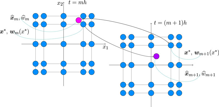
FIGURE 1. Evolution of the spatial variable and the corresponding PDF for two consecutive time steps related to the fixed Chebyshev grid in the case of two dimensions.
Note that, according to our splitting scheme, we solve the convection part eq. 14 after the corresponding diffusion eq. 13, and hence the initial condition
Hence our solution strategy for convection equation is the following. For the given spatial grid point
backward in time to find the corresponding point
An important contribution of this paper is an indication of the possibility and a practical implementation of the usage of the multidimensional CAM in the TT-format to recover a supposedly low-rank tensor
3 Low-Rank Representation
There has been much interest lately in the development of data-sparse tensor formats for high-dimensional problems. A very promising tensor format is provided by the tensor train (TT) approach (Oseledets and Tyrtyshnikov, 2009; Oseledets, 2011), which was proposed for compact representation and approximation of high-dimensional tensors. It can be computed via standard decompositions (such as SVD and QR-decomposition) but does not suffer from the curse of dimensionality7.
In many analytical considerations and practical cases a tensor is given implicitly by a procedure enabling us to compute any of its elements, so the tensor appears rather as a black box. For example, to construct the convection part of PDF (i.e., the tensor
In this section we describe the properties of the TT-format and multidimensional CAM that are necessary for efficient solution of our problem, as well as the specific features of the practical implementation of interpolation by the Chebyshev polynomials in terms of the TT-format and CAM.
3.1 Tensor Train Format
A tensor
where
where
where the slices of the TT-cores
The benefit of the TT-decomposition is the following. Storage of the TT-cores
The detailed description of the TT-format and linear algebra operations in terms of this format8 is given in works (Oseledets and Tyrtyshnikov, 2009; Oseledets, 2011). It is important to note that for a given tensor
but a procedure of the tensor approximation in the full format is too costly, and is even impossible for large dimensions due to the curse of dimensionality. Therefore more efficient algorithms like CAM are needed to quickly construct the tensor in the low rank TT-format.
3.2 Cross Approximation Method
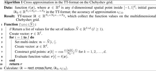
The CAM allows to construct a TT-approximation of the tensor with prescribed accuracy
The CAM constructs a TT-approximation
3.3 Multidimensional Interpolation
As was discussed in the previous sections, we discretize the FPE on the multidimensional Chebyshev grid and interpolate solution of the first diffusion equation in the splitting scheme eq. 13 by the Chebyshev polynomials to obtain its values on custom spatial points (different from the grid nodes) and then perform efficient trajectory integration of the convection eq. 14.
The desired interpolation may be constructed from solution of the system of eq. 22 in terms of the FFT (Trefethen, 2000), but for the high dimension numbers we have the exponential growth of computational complexity and memory consumption, hence it is very promising to construct tensor of the nodal values and the corresponding interpolation coefficients in the TT-format.
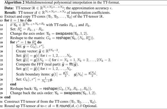
Consider a TT-tensor
In this Algorithm we use standard linear algebra operations
For the known tensor
We’ll call the corresponding function as
4 Detailed Algorithms
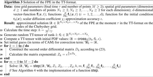
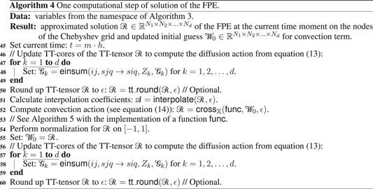
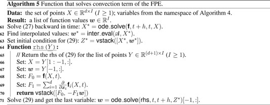
In Algorithms 3, 4 and 5 we combine the theoretical details discussed in the previous sections of this work and present the final calculation scheme for solution of the multidimensional FPE in the TT-format, using CAM (function
We denote by
5 Numerical Examples
In this section we illustrate the proposed computational scheme, which was presented above, with the numerical experiments. All calculations were carried out in the Google Colab cloud interface11 with the standard configuration (without GPU support).
Firstly we consider an equation with a linear convection term—Ornstein-Uhlenbeck process (OUP) (Vatiwutipong and Phewchean, 2019) in one, three and five dimensions. For the one-dimensional case, which is presented for convention, we only solve equation using the dense format (not TT-format), hence the corresponding results are used to verify the general correctness and convergence properties of the proposed algorithm, but not its efficiency. In the case of the multivariate problems we use the proposed tensor based solver, which operates in accordance with the algorithm described above. To check the results of our computations, we use the known analytic stationary solution for the OUP, and for the one-dimensional case we also perform comparison with constructed analytic solution at any time moment.
Then we consider more complicated dumbbell problem (Venkiteswaran and Junk, 2005) which may be represented as a three-dimensional FPE with a nonlinear convection term. For this case we consider the Kramer expression and compare our computation results with the results from another works for the same problem.
In the numerical experiments we consider the spatial region
where parameter s is selected as
We compute the value
5.1 Numerical Solution of the Ornstein-Uhlenbeck Process
Consider FPE of the form eq. 6 in the d-dimensional case with
where
• mean vector is
• covariance matrix is
and, in our case as noted above
• transitional PDF is
• stationary solution is
where matrix
• the (multivariate) OUP at any time is a (multivariate) normal random variable;
• the OUP is mean-reverting (the solution tends to its long-term mean
5.1.1 One-Dimensional Process
Let consider the one-dimensional (
We can calculate the analytic solution in terms of only spatial variable and time via integration of the transitional PDF eq. 41
Accurate computations lead to the following formula
where
Using the formulas eq. 42 and eq. 43 we can represent a stationary solution for the one-dimensional case in the explicit form
We perform computation for
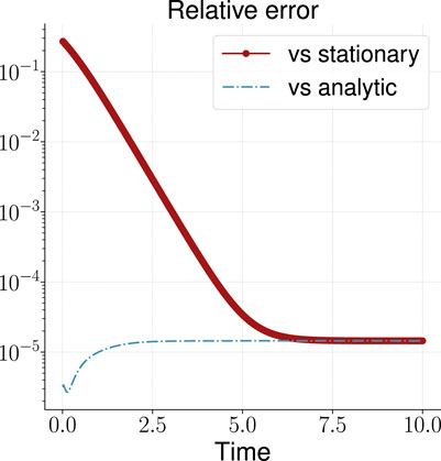
FIGURE 2. Relative error of the calculated solution vs known analytic and stationary solutions for the one-dimensional OUP.
5.1.2 Three-Dimensional Process
Our next example is the three-dimensional (
When carrying out numerical calculation, we select
The result is shown in Figure 3. As can be seen, the TT-rank12 remains limited, and the accuracy of the solution over time grows, reaching
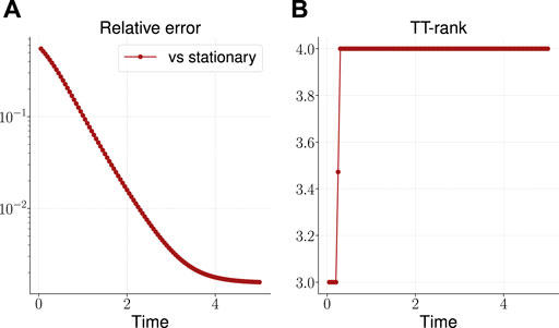
FIGURE 3. Relative error of the calculated solution vs known stationary solution (A) and the effective TT-rank (B) for the three-dimensional OUP.
To evaluate the efficiency of the proposed algorithm in the TT-format, we also solve these three-dimensional OUP, using dense format (as for the one-dimensional case, all arrays are presented in its full form). The corresponding calculation took about 376 s, so in this case we have an acceleration of calculations by more than an order of magnitude.
5.1.3 Five-Dimensional Process
This multidimensional case is considered in the same manner as the previous one. We select the following parameters
We select the same values as in the previous example for the CAM accuracy (
The results are presented on the plots on Figure 4. The TT-rank of the solution remains limited and reaches the value 4.5 at the end time step, and the solution accuracy reaches almost
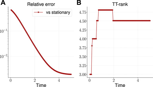
FIGURE 4. Relative error of the calculated solution vs known stationary solution (A) and the effective TT-rank (B) for the five-dimensional OUP.
5.2 Numerical Solution of the Dumbbell Problem
Now consider a more complex non-linear example corresponding to the three-dimensional (
where
Making simple calculations (taking into account the specific form of the matrix A), we get explicit expressions for the function and the required partial derivatives (
Next, we consider the Kramer expression
and as the values of interest (as in the works (Venkiteswaran and Junk, 2005; Dolgov et al., 2012)) we select
During the calculations we used the following solver parameters:
• the accuracy of the CAM is
• the number of time grid points is 100;
• the number of grid points along each of the spatial dimensions is 60.
The results are presented on the plots on Figure 5. The time to build the solution was about 200 s (also additional time was required to calculate the values
with the corresponding results from (Dolgov et al., 2012)14, and we get the following values for relative errors
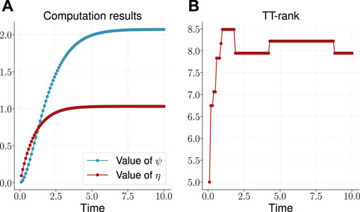
FIGURE 5. Computed values (A) and the effective TT-rank (B) for the three-dimensional dumbbell problem.
6 Related Works
The problem of uncertainty propagation through nonlinear dynamical systems subject to stochastic excitation is given by the FPE, which describes the evolution of the PDF, and has been extensively studied in the literature. A number of numerical methods such as the path integral technique (Wehner and Wolfer, 1983; Subramaniam and Vedula, 2017), the finite difference and the finite element method (Kumar and Narayanan, 2006; Pichler et al., 2013) have been proposed to solve the FPE.
These methods inevitably require mesh or associated transformations, which increase the amount of computation. The problem becomes worse when the system dimension increases. To maintain accuracy in traditional discretization based numerical methods, the number of degrees of freedom of the approximation, i.e. the number of unknowns, grows exponentially as the dimensionality of the underlying state-space increases.
On the other hand, the Monte Carlo method, that is common for such kind of problems (Kikuchi et al., 1991; Küchlin and Jenny, 2017), has slow rate of convergence, causing it to become computationally burdensome as the underlying dimensionality increases. Hence, the so-called curse of dimensionality fundamentally limits the use of the FPE for uncertainty quantification in high dimensional systems.
In recent years, low-rank tensor approximations have become especially popular for solving multidimensional problems in various fields of knowledge (Cichocki et al., 2016). However, for the FPE, this approach is not yet widely used. We note the works (Dolgov et al., 2012; Sun and Kumar, 2014; Sun and Kumar, 2015; Dolgov, 2019; Fox et al., 2020) in which the low-rank TT-decomposition was proposed for solution of the multidimensional FPE. In these works, the differential operator and the right-hand side of the system are represented in the form of TT-tensor. Moreover, in paper (Dolgov et al., 2012) the joint discretization of the solution in space-time is considered. The difference of our approach from these works is its more explicit iterative form for time integration, as well as the absence of the need to represent the right hand side of the system in a low-rank format, which allows to use this approach in machine learning applications.
7 Conclusion
In this paper we proposed the novel numerical scheme for solution of the multidimensional Fokker–Planck equation, which is based on the Chebyshev interpolation and spectral differentiation techniques as well as low rank tensor approximations, namely, the tensor train decomposition and cross approximation method, which in combination make it possible to drastically reduce the number of degrees of freedom required to maintain accuracy as dimensionality increases.
The proposed approach can be used for the numerical analysis of uncertainty propagation through nonlinear dynamical systems subject to stochastic excitations, and we demonstrated its effectiveness on a number of multidimensional problems, including Ornstein-Uhlenbeck process and dumbbell model.
As part of the further development of this work, we plan to conduct more rigorous estimates of the convergence of the proposed scheme, as well as formulate a set of heuristics for the optimal choice of number of time and spatial grid points and tensor train rank. Another promising direction for further research is the application of established approaches and developed solver to the problem of density estimation for machine learning models.
Data Availability Statement
Program code, input data and calculation results can be found here: https://github.com/AndreiChertkov/fpcross
Author Contributions
IO contributed to general formulation of the problem and formulation of the preliminary version of the algorithm. AC contributed to development of the final version of algorithms and program code, carrying out numerical experiments.
Funding
The work was supported by Ministry of Science and Higher Education grant No. 075-10-2021-068.
Conflict of Interest
The authors declare that the research was conducted in the absence of any commercial or financial relationships that could be construed as a potential conflict of interest.
Publisher’s Note
All claims expressed in this article are solely those of the authors and do not necessarily represent those of their affiliated organizations, or those of the publisher, the editors and the reviewers. Any product that may be evaluated in this article, or claim that may be made by its manufacturer, is not guaranteed or endorsed by the publisher.
Footnotes
1Vectors and matrices are denoted hereinafter by lower case bold letters (
2The code is publicly available from https://github.com/AndreiChertkov/fpcross.
3We use notation
4We suppose that for each spatial dimension the variable x varies within
5By tensors we mean multidimensional arrays with a number of dimensions d (
6Note that for the case
7By the full format tensor representation or uncompressed tensor we mean the case, when one calculates and saves in the memory all tensor elements. The number of elements of an uncompressed tensor (hence, the memory required to store it) and the amount of operations required to perform basic operations with such tensor grows exponentially in the dimensionality, and this problem is called the curse of dimensionality.
8All basic operations in the TT-format are implemented in the ttpy python package https://github.com/oseledets/ttpy and its MATLAB version https://github.com/oseledets/TT-Toolbox.
9An exact TT-representation exists for the given full tensor
10Note that in Algorithm 4 we use the solution of the convection part from the previous time step (
11Actual links to the corresponding Colab notebooks are available in our public repository https://github.com/AndreiChertkov/fpcross.
12Hereinafter, we present effective TT-rank of the computation result. For TT-tensor
13This choice of parameters corresponds to the problem of polymer modeling from the work (Venkiteswaran and Junk, 2005). In the corresponding model, the molecules of the polymer are represented by beads and interactions are indicated by connecting springs. Accordingly, for the case of only two particles we come to the dumbbell problem, which can be mathematically written in the form of the FPE.
14As values for comparison, we used the result of the most accurate calculation from work (Dolgov et al., 2012), within which
References
Chen, R. T., and Duvenaud, D. (2019). Neural Networks with Cheap Differential Operators. New York, NY: arXiv preprint arXiv:1912.03579.
Chen, T. Q., Rubanova, Y., Bettencourt, J., and Duvenaud, D. K. (2018). Neural Ordinary Differential Equations. Adv. Neural Inf. Process. Syst., 6571–6583.
Cichocki, A., Lee, N., Oseledets, I., Phan, A.-H., Zhao, Q., and Mandic, D. P. (2016). Tensor Networks for Dimensionality Reduction and Large-Scale Optimization: Part 1 Low-Rank Tensor Decompositions. FNT Machine Learn. 9, 249–429. doi:10.1561/2200000059
Dolgov, S., and Savostyanov, D. (2020). Parallel Cross Interpolation for High-Precision Calculation of High-Dimensional Integrals. Comp. Phys. Commun. 246, 106869. doi:10.1016/j.cpc.2019.106869
Dolgov, S. V. (2019). A Tensor Decomposition Algorithm for Large Odes with Conservation Laws. Comput. Methods Appl. Math. 19, 23–38. doi:10.1515/cmam-2018-0023
Dolgov, S. V., Khoromskij, B. N., and Oseledets, I. V. (2012). Fast Solution of Parabolic Problems in the Tensor Train/Quantized Tensor Train Format with Initial Application to the Fokker--Planck Equation. SIAM J. Sci. Comput. 34, A3016–A3038. doi:10.1137/120864210
Fox, C., Dolgov, S., Morrison, M. E., and Molteno, T. C. (2020). Grid Methods for Bayes-Optimal Continuous-Discrete Filtering and Utilizing a Functional Tensor Train Representation. Inverse Probl. Sci. Eng., 1–19. doi:10.1080/17415977.2020.1862109
Glowinski, R., Osher, S. J., and Yin, W. (2017). Splitting Methods in Communication, Imaging, Science, and Engineering. Springer.
Grathwohl, W., Chen, R. T., Bettencourt, J., Sutskever, I., and Duvenaud, D. (2018). Ffjord: Free-form Continuous Dynamics for Scalable Reversible Generative Models. arXiv preprint arXiv:1810.01367.
Kidger, P., Foster, J., Li, X., Oberhauser, H., and Lyons, T. (2021). Neural Sdes as Infinite-Dimensional gans. arXiv preprint arXiv:2102.03657.
Kikuchi, K., Yoshida, M., Maekawa, T., and Watanabe, H. (1991). Metropolis Monte Carlo Method as a Numerical Technique to Solve the Fokker-Planck Equation. Chem. Phys. Lett. 185, 335–338. doi:10.1016/s0009-2614(91)85070-d
Küchlin, S., and Jenny, P. (2017). Parallel Fokker-Planck-DSMC Algorithm for Rarefied Gas Flow Simulation in Complex Domains at All Knudsen Numbers. J. Comput. Phys. 328, 258–277. doi:10.1016/j.jcp.2016.10.018
Kumar, P., and Narayanan, S. (2006). Solution of Fokker-Planck Equation by Finite Element and Finite Difference Methods for Nonlinear Systems. Sadhana 31, 445–461. doi:10.1007/bf02716786
Oseledets, I., and Tyrtyshnikov, E. (2010). Tt-cross Approximation for Multidimensional Arrays. Linear Algebra its Appl. 432, 70–88. doi:10.1016/j.laa.2009.07.024
Oseledets, I. V. (2010). Approximation of $2^d\times2^d$ Matrices Using Tensor Decomposition. SIAM J. Matrix Anal. Appl. 31, 2130–2145. doi:10.1137/090757861
Oseledets, I. V. (2011). Tensor-train Decomposition. SIAM J. Sci. Comput. 33, 2295–2317. doi:10.1137/090752286
Oseledets, I. V., and Tyrtyshnikov, E. E. (2009). Breaking the Curse of Dimensionality, or How to Use Svd in many Dimensions. SIAM J. Sci. Comput. 31, 3744–3759. doi:10.1137/090748330
Pichler, L., Masud, A., and Bergman, L. A. (2013). “Numerical Solution of the Fokker-Planck Equation by Finite Difference and Finite Element Methods-A Comparative Study,” in Computational Methods in Stochastic Dynamics (Springer), 69–85. doi:10.1007/978-94-007-5134-7_5
Savostyanov, D., and Oseledets, I. (2011). “Fast Adaptive Interpolation of Multi-Dimensional Arrays in Tensor Train Format,” in The 2011 International Workshop on Multidimensional (nD) Systems (IEEE), 1–8. doi:10.1109/nds.2011.6076873
Singh, R., Ghosh, D., and Adhikari, R. (2018). Fast Bayesian Inference of the Multivariate Ornstein-Uhlenbeck Process. Phys. Rev. E 98, 012136. doi:10.1103/PhysRevE.98.012136
Subramaniam, G. M., and Vedula, P. (2017). A Transformed Path Integral Approach for Solution of the Fokker-Planck Equation. J. Comput. Phys. 346, 49–70. doi:10.1016/j.jcp.2017.06.002
Sun, Y., and Kumar, M. (2015). A Numerical Solver for High Dimensional Transient Fokker-Planck Equation in Modeling Polymeric Fluids. J. Comput. Phys. 289, 149–168. doi:10.1016/j.jcp.2015.02.026
Sun, Y., and Kumar, M. (2014). Numerical Solution of High Dimensional Stationary Fokker-Planck Equations via Tensor Decomposition and Chebyshev Spectral Differentiation. Comput. Math. Appl. 67, 1960–1977. doi:10.1016/j.camwa.2014.04.017
Tyrtyshnikov, E. (2000). Incomplete Cross Approximation in the Mosaic-Skeleton Method. Computing 64, 367–380. doi:10.1007/s006070070031
Vatiwutipong, P., and Phewchean, N. (2019). Alternative Way to Derive the Distribution of the Multivariate Ornstein-Uhlenbeck Process. Adv. Differ. Equ 2019, 276. doi:10.1186/s13662-019-2214-1
Venkiteswaran, G., and Junk, M. (2005). A QMC Approach for High Dimensional Fokker-Planck Equations Modelling Polymeric Liquids. Mathematics Comput. Simulation 68, 43–56. doi:10.1016/j.matcom.2004.09.002
Keywords: fokker-planck equation, probability density function, tensor train format, cross approximation, chebyshev polynomial, ornstein-uhlenbeck process, dumbbell model
Citation: Chertkov A and Oseledets I (2021) Solution of the Fokker–Planck Equation by Cross Approximation Method in the Tensor Train Format. Front. Artif. Intell. 4:668215. doi: 10.3389/frai.2021.668215
Received: 15 February 2021; Accepted: 29 June 2021;
Published: 02 August 2021.
Edited by:
Evangelos Papalexakis, University of California, Riverside, United StatesReviewed by:
Devin Matthews, Southern Methodist University, United StatesPrakash Vedula, University of Oklahoma, United States
Copyright © 2021 Chertkov and Oseledets. This is an open-access article distributed under the terms of the Creative Commons Attribution License (CC BY). The use, distribution or reproduction in other forums is permitted, provided the original author(s) and the copyright owner(s) are credited and that the original publication in this journal is cited, in accordance with accepted academic practice. No use, distribution or reproduction is permitted which does not comply with these terms.
*Correspondence: Andrei Chertkov, YS5jaGVydGtvdkBza29sdGVjaC5ydQ==