 Peter Taraba
- Independent Researcher, Fort Lauderdale, FL, United States
We derive blending coefficients for the optimal blend of multiple independent prediction models with normal (Gaussian) distribution as well as the variance of the final blend. We also provide lower and upper bound estimation for the final variance and we compare these results with machine learning with counts, where only binary information (feature says yes or no only) is used for every feature and the majority of features agreeing together make the decision.
Introduction
Participants of the Netflix competition used model blending heavily—refer to, for example Töscher et al. (2009), Amatriain (2013), Xiang and Yang (2009), Coscrato et al. (2020), Koren (2009), Jahrer et al. (2010), and Bothos et al. (2011). Ensemble modeling (blending) was popular not only in Netflix competition but is used also on other machine learning problems such as image processing, for example for CIFAR-10 dataset, refer to Abouelnaga et al. (2016) and Bruno et al. (2022), for the MNIST dataset refer to Ciresan et al. (2011). Ensemble modeling is used also in many other fields, for example, refer to Schuhen et al. (2012) and Ardabili et al. (2020). In this study, we derive blending coefficients based on variances of different models with only the assumption of model independence. While the formula for the final variance of the blended model and its coefficients is already derived in Kay (1993) without a proof (Equations 6.7 and 6.8 in chapter 6.4), we provide proofs both for the formula for blending coefficients and the variance of the combined model as well as the lower and upper bound estimate for the final variance based on the minimal and maximal variance of all the combined models. We also compare these results with machine learning with counts, where only binary information is used from the features to make the decision, in the last section and show very similar conclusions.
Let ŷk,j be a prediction of model k ∈ [1, N] for element j ∈ [1, M], where N is the number of different independent models and M is the number of measurements we have:
where yj is an expected prediction and rk,j is a random variable with normal distribution , which has a zero average (the expected value of the variable is 0). In this study, we derive optimal blending coefficients αk such that the blended prediction ŷB is optimal:
with minimum variance , where .
Blending two independent models
Here we present two independent models
where and . We derive for which we get the optimal blending model
It is well-known fact that a random variable combining two random variables αR1 + (1 − α)R2, where , and R1 and R2 are independent, has a normal distribution , where . For the mean we get:
and for the variance we get:
Finally as R1 and R2 are independent (covariance is zero), we can write:
To find the optimal (we are looking for minimal value and function is convex with one minimum as we have only α0, α1, and α2 dependencies—quadratic function and ) blending parameter, we compute where a partial derivative of the new variance of the blended model is zero:
from which
and the optimal variance will be:
In Figure 1, we show how the variance is changing for different blending parameters α. Script is in Appendix 1. Blue dot—optimal value of blending parameter α matches simulation (minimal value for variance).
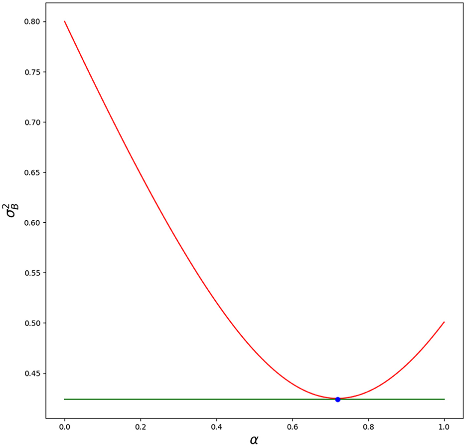
Figure 1. Red line—variance for different α. Green line—optimal variance . Blue dot—optimal α with its value . Python script is in Appendix 1.
Blending three independent models
Now, we consider three independent models
where , , and .
Here, we blend optimally the first two models from the previous section:
where and then we find the blending parameter for ŷ3,j and ŷ4,j such that
Based on the Equation (1), we get
Plugging this back into the Equation (3), we get
which is symmetrical, meaning model combination order is irrelevant. Finally for , , , we get:
Combining the second and third models first and then combining the result with the first model would lead to the same optimal blending parameters. The order of the combination is inconsequential. Additionally, for the final variance, we get from Equation (2)
In Figure 2, we show how variance is changing for different blending parameters α1 and α2 and α3 = 1 − α1 − α2. The script is in Appendix 2. Blue dot—the optimal value of blending parameters (α1, α2, 1 − α1 − α2) matches the simulation (minimal value for variance).
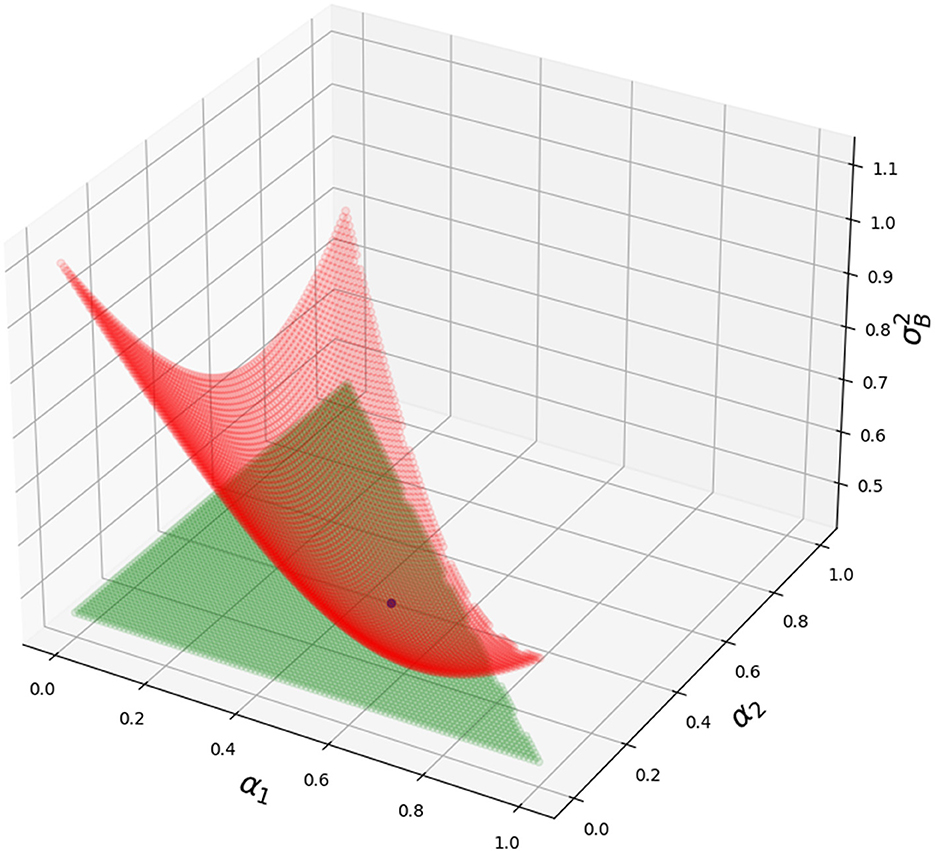
Figure 2. Grid consisting of red dots—variance for different α1 and α2. Grid consisting of green dots—optimal variance . Blue dot—optimal α1 and α2 and 1 − α1 − α2 with its value . Python script is in Appendix 2.
Blending N independent models
Now that we have formulas for two and three different models, we prove formulas for N independent models with normal distributions:
where . We combine these models as follows:
where and αk > 0 for k ∈ [1, N].
First, we show model independence is still needed.
Lemma 1. Having N independent models with normal distributions for k ∈ [1, N], when combined as , variance of RB is .
Proof.
As models are independent (covariance is zero for l ≠ k), we get
which ends the proof.
Theorem 2. Having N independent models with normal distributions for k ∈ [1, N], we get an optimal blend with parameters
and these independent models form normal distribution , which has variance
Proof. For N = 2, we have shown it in Section 2. Now we use induction, if it is true for N, then it is true also for N + 1.
Remark. We have shown this also for three models in Section 3, but as for induction it is not needed, Section 3 is only a motivational section for how to derive final formulas for N models.
We combine two normal distributions (assuming it is true for N) and . From Equation (2), (lemma 1 is incorporated in this equation) we get
and hence, we have shown optimal variance is valid for N + 1. Now we must show the same for the optimal coefficients. From Equation (1), we get
and hence,
which proves . Finally to show the same for for k ∈ [1, N]:
which ends the proof.
Going to infinity
If we can generate infinite independent models with distributions (same variance), the final variance will be
which means we can combine all these models to get a perfect prediction with no errors. Naturally, creating an infinite amount of independent models (with covariances zero) is a difficult if not impossible task in real applications.
Theorem 3. Having N independent models with normal distributions for k ∈ [1, N] and their variances , where is their maximum variance, combining them optimally with coefficients from the theorem 2, their combined variance is .
Proof. We use induction again. For N = 2, we get
This is true as
because
and
Now if it is true for N, then it is true also for N + 1. If
then
That is true as
because
as both - this
and this
are true, which ends the proof.
This proof means, that if we combine infinite independent models with distributions , where variance , we get variance:
Combining infinite independent models with bounded variances from above leads to perfect prediction with variance zero.
It can be shown the same way as in Theorem 3 that combined variance is bounded also from below (as the proof is almost identical we avoid it here). If all distributions for k ∈ [1, N] have their variance in interval for k ∈ [1, N], then their combined variance will be in interval .
Similar conclusion with machine learning with counts
When it comes to using only counts (feature says yes or no only) in machine learning for predictions, as it is shown in Taraba (2021) (see section 7) on a nine-features example, we can come to the same conclusion as in the previous chapter that an infinite amount of features can lead to perfect prediction with no error. While the previous approach is statistical, machine learning with counts uses Pascal's triangle and binomial raised to infinity to show this. We use the binomial expansion
where p is the probability of features to be correct. As we want to have an odd amount of features to be able to make a decision purely on the counts (feature says yes or no), we will replace n with 2k + 1
This can be split into two parts, one with probability when the majority of features are correct Pcorrect and one with probability when the majority of features are incorrect:
where
and
To show that an infinite amount of features can lead to perfect prediction, we have to show that Pcorrect with the majority of features correct (at least k + 1 of them correct) goes to 1 for all p ∈ (0.5, 1]
We start by showing the simpler case first and that is when p = 0.5 then Pcorrect and Pincorrect are equal and Pcorrect = Pincorrect = 0.5. To show this, we can write
and
and those are equal as , because for i ∈ {0, 1, …, k}. As Pcorrect,p = 0.5 = Pincorrect,p = 0.5 and their sum is 1 it follows that
and hence,
Now that we have shown what happens when p = 0.5, we show the main limit theorem for p ∈ (0.5, 1].
Theorem 4. for all p ∈ (0.5, 1].
Proof. To show that for all p ∈ (0.5, 1], we will show instead that and as their sum is 1, will follow.
First, we can rewrite as
It is obvious that the numbers in the pascal triangle are decreasing when starting after the middle:
for i ∈ 0, 1, …, k − 1, and hence, we can write
As p is in p ∈ (0.5, 1], then , and hence, we can write
With that we can finally look at the original limit and write
As for p ∈ (0.5, 1] as , we can write
Now we look at . We can take a member and compare it with r′ = r + 1 follower by division
for all r ≥ 0 and p ∈ (0.5, 1] as p(1 − p) ∈ [0, 0.25). This means we are multiplying a finite number , which is in interval [0, 1], infinitely many times with a number larger or equal than 0 and smaller than 1, hence
and hence, the original limit
as well. As , it follows that
Remark. It is worth mentioning that p is fixed and chosen from the interval (0.5, 1], and we are not looking at the limit of p → 0.5, but the limit of k → ∞. For p = 0.5, we already know that Pcorrect,p = 0.5 = Pincorrect,p = 0.5 = 0.5.
As
it follows that , which ends the proof.
This could be summarized for all p ∈ [0, 1] in Figure 3 as
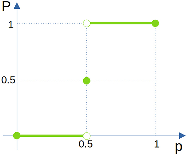
Figure 3. Different outcomes for Pcorrect for different p intervals when k is going to ∞.
This can be understood intuitively by plotting Pcorrect with increasing k in Figure 4.
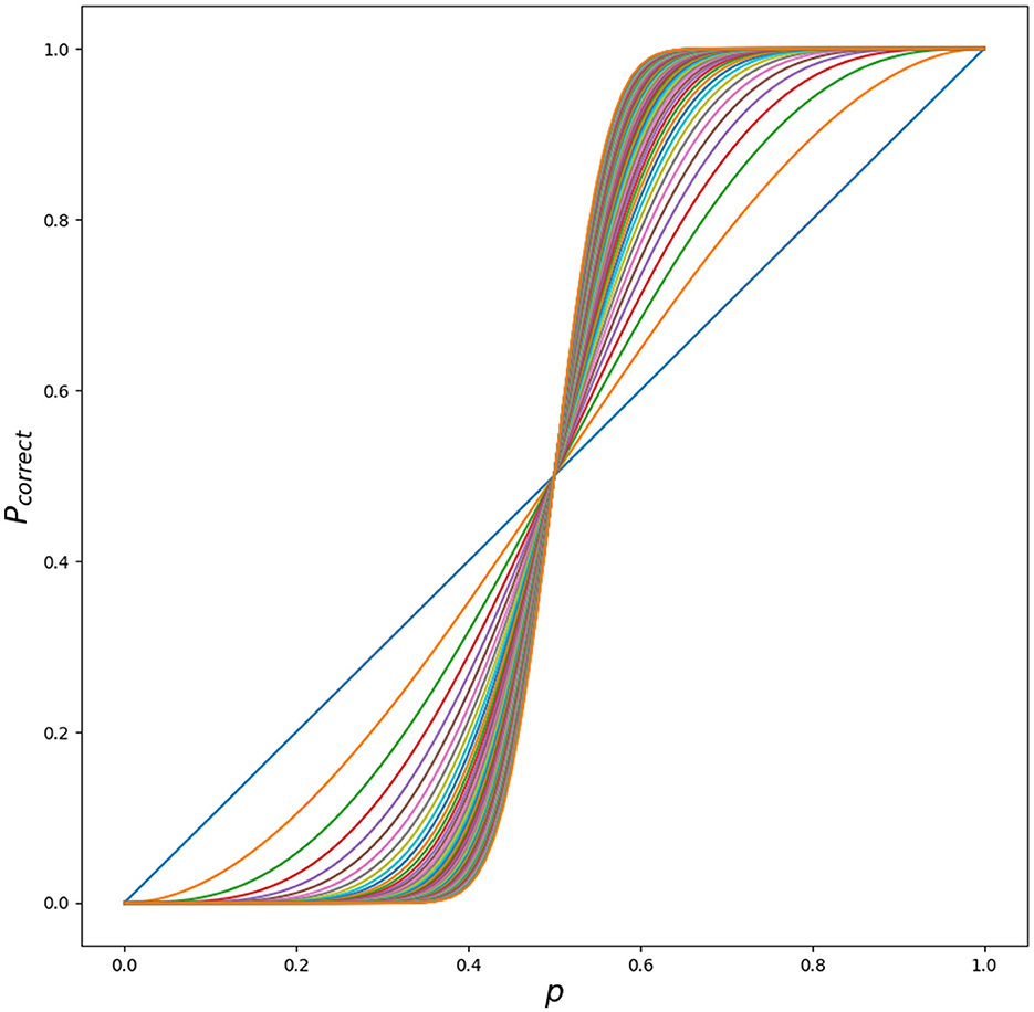
Figure 4. Different outcomes for Pcorrect for different p ∈ [0.0, 1] with increasing k ∈ [0, …, 51]. Python script is in Appendix 3.
It is worth mentioning that with weak features with p = 0.52, and only n = 15001 of them (no need to go to infinity), Pcorrect is already around 1 (see Figure 5).
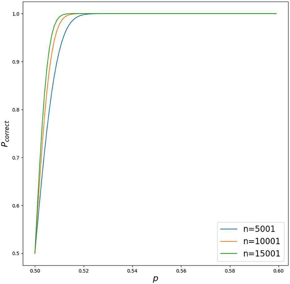
Figure 5. Different outcomes for Pcorrect for different p ∈ [0.5, 0.6] with increasing n for n ∈ {5001, 10001, 15001}. Python script is in Appendix 4.
As next, we show that Pcorrect increases, if any of the probability of the features increases its value . For case k = 0 (n = 1), this is simple, as
For three features, it is also trivial as
as it can be re-written to independent part and dependent part
and from that, it immediately follows that Pcorrect(new) > Pcorrect(old) as and . To show this for the general case, not only for cases k ∈ {0, 1} (n = 2k + 1 ∈ {1, 3}), we first write the general formula:
This can be re-written into two parts once again, Pcorrect, when the majority of features say yes—are correct, and Pincorrect, when the majority of features say no—are incorrect.
where
Theorem 5. Increasing the probability of one of the features increases final correct probability of all features, .
Proof. We show this for increasing the first probability, as probabilities can be re-ordered and their order does not matter for the final correct probability.
Now again, as with example k = 1, n = 3, Pcorrect can be split into independent and dependent part. The dependent part will only contain and no as for every there is also the exact same case with , where even more features are correct and those two can be joined and hence it belongs to the independent part. Hence,
and
where PI and PD are fixed and non-negative (as all pi ≥ 0 and (1 − pi) ≥ 0) and dependent on p2, …, p2k+1 and hence as , which ends the proof.
Theorem 6. , where pmin = min{p1, p2, …, p2k+1}.
Proof. This proof directly follows from using the Theorem 5 multiple times by increasing every probability one at a time from the initial value pmin:
which ends the proof.
Theorems 6 and 4 were needed in order to be able to say, that combining an infinite amount of features with their probabilities pi ∈ (0.5, 1] (min{p1, …, p2k+1, …} > 0.5) will lead to perfect prediction with no error for machine learning with counts, as it was in previous Section 5 when looking at the same problem from the statistical point of view (Gaussian distributions). It is important to say once again that these separate probabilities pi have to be independent, as otherwise Equation (4) would not be valid.
Conclusion and discussion
We have derived blending coefficients for the ensemble of multiple independent prediction models with normal error distribution. This manuscript was mainly inspired by a Netflix competition, in which in the final stages of competition multiple teams joined their efforts to increase the accuracy of their final predictor and blending turned out to be essential to win the competition in a very short time during the final stage. This method was not only used in the Netflix competition but is used for other datasets in machine learning, such as MNIST and CIFAR-10 for image processing. We have also shown that having an infinite amount of independent predictors with their variances bounded from above is sufficient to achieve perfect prediction. While deep learning is very popular these days, one should not forget to include more features (going wider) when in need of improvement in accuracy.
Looking at a similar problem and more specifically machine learning with counts, where we only count how many features are for and against and make a decision based on a voting mechanism and a majority vote winner, we have shown once again, that an infinite amount of independent features will lead to perfect prediction when using only features which have >50% of accuracy.
Naturally, independent features in practice are hard to find and further the study could be made on how to convert dependent (correlated) features into independent in order to achieve as high accuracy as possible, or how to combine these dependent features together and what theoretical accuracies can be achieved. It could be also of interest how to combine features, which are not binary (for and against features), but have more than two possible outcomes.
Data availability statement
The original contributions presented in the study are included in the article/Supplementary material, further inquiries can be directed to the corresponding author.
Author contributions
The author confirms being the sole contributor of this work and has approved it for publication.
Acknowledgments
We would like to thank the reviewers for their suggestions and comments which led to the improvement of the manuscript.
Conflict of interest
The author declares that the research was conducted in the absence of any commercial or financial relationships that could be construed as a potential conflict of interest.
Publisher's note
All claims expressed in this article are solely those of the authors and do not necessarily represent those of their affiliated organizations, or those of the publisher, the editors and the reviewers. Any product that may be evaluated in this article, or claim that may be made by its manufacturer, is not guaranteed or endorsed by the publisher.
Supplementary material
The Supplementary Material for this article can be found online at: https://www.frontiersin.org/articles/10.3389/frai.2023.1144886/full#supplementary-material
References
Abouelnaga, Y., Ali, O. S., Rady, H., and Moustafa, M. (2016). “Cifar-10: KNN-based ensemble of classifiers,” in 2016 International Conference on Computational Science and Computational Intelligence (CSCI) (Las Vegas, NV), 1192–1195.
Amatriain, X. (2013). “Big & personal: data and models behind netflix recommendations,” in BigMine '13 (Chicago, IL).
Ardabili, S., Mosavi, A., and Várkonyi-Kóczy, A. R. (2020). “Advances in machine learning modeling reviewing hybrid and ensemble methods,” in Engineering for Sustainable Future, ed A. R. Várkonyi-Kóczy (Cham: Springer International Publishing), 215–227.
Bothos, E., Christidis, K., Apostolou, D., and Mentzas, G. (2011). “Information market based recommender systems fusion,” in Proceedings of the 2nd International Workshop on Information Heterogeneity and Fusion in Recommender Systems, HetRec '11 (New York, NY: Association for Computing Machinery), 1–8.
Bruno, A., Moroni, D., and Martinelli, M. (2022). Efficient Adaptive Ensembling for Image Classification. Technical report, ISTI Working Paper, 2022. Consiglio Nazionale delle Ricerche.
Ciresan, D. C., Meier, U., Gambardella, L. M., and Schmidhuber, J. (2011). “Convolutional neural network committees for handwritten character classification,” in 2011 International Conference on Document Analysis and Recognition, 1135–1139.
Coscrato, V., de Almeida Inácio, M. H., and Izbicki, R. (2020). The NN-stacking: feature weighted linear stacking through neural networks. Neurocomputing 399, 141–152.
Jahrer, M., Töscher, A., and Legenstein, R. (2010). “Combining predictions for accurate recommender systems,” in Proceedings of the 16th ACM SIGKDD International Conference on Knowledge Discovery and Data Mining, KDD '10 (New York, NY: Association for Computing Machinery), 693–702.
Kay, S. M. (1993). Fundamentals of Statistical Signal Processing: Estimation Theory. Prentice-Hall, Inc.
Schuhen, N., Thorarinsdottir, T. L., and Gneiting, T. (2012). Ensemble model output statistics for wind vectors. Month. Weath. Rev. 140, 3204–3219. doi: 10.1175/MWR-D-12-00028.1
Taraba, P. (2021). Linear regression on a set of selected templates from a pool of randomly generated templates. Mach. Learn. Appl. 6:100126. doi: 10.1016/j.mlwa.2021.100126
Keywords: blending of independent models, normal distributions, machine learning with counts, Gaussians, going wider
Citation: Taraba P (2023) Optimal blending of multiple independent prediction models. Front. Artif. Intell. 6:1144886. doi: 10.3389/frai.2023.1144886
Received: 15 January 2023; Accepted: 06 February 2023;
Published: 24 February 2023.
Edited by:
Georgios Leontidis, University of Aberdeen, United KingdomReviewed by:
Kristina Sutiene, Kaunas University of Technology, LithuaniaJolita Bernatavičienė, Vilnius University, Lithuania
Copyright © 2023 Taraba. This is an open-access article distributed under the terms of the Creative Commons Attribution License (CC BY). The use, distribution or reproduction in other forums is permitted, provided the original author(s) and the copyright owner(s) are credited and that the original publication in this journal is cited, in accordance with accepted academic practice. No use, distribution or reproduction is permitted which does not comply with these terms.
*Correspondence: Peter Taraba,  dGFyYWJhLnBldGVyQG1haWwuY29t