Abstract
This article presents a pragmatic framework for time-sensitive analysis of behavioral RCTs using sequence methods and Markov modeling. The focus is not methodological novelty but translation: we map common policy questions to appropriate temporal tools, provide a reporting checklist for transparency, and show how estimates become implementable rules for booster timing, triage, and exit. We position sequence analysis alongside multi-state hazards, HMMs, SMART/MRT, and g-methods, and we introduce an openly documented R package, sequenceRCT, that operationalises the end-to-end workflow with uncertainty quantification and reproducible outputs. A simulated illustration demonstrates interpretation and decision use, with ablations and a counterfactual booster vignette. We extend the framework to personalized interventions–where state-specific individual treatment effects are difficult to detect–and to reinforcement learning, where sequence-derived state spaces, empirical kernels, and off-policy evaluation support safe policy learning. We conclude with a staged validation agenda on existing datasets.
1 Introduction
Behavioral public policy now operates in settings where the temporal texture of human behavior matters as much as average endline outcomes. Policies are rolled out through repeated prompts, incentives vary over time, participants cycle through adherence and relapse, and digital delivery makes it possible to intervene and to measure at fine time scales. Against this background, a central question is no longer only whether an intervention works on average, but how people traverse behavioral states over time, when they are most vulnerable to backsliding, and how long gains persist without further support.
Standard RCT analyses often cannot answer those questions directly. Regression and growth-curve models, for instance, are powerful for estimating average effects and their moderators, yet they compress time into trends or a handful of observation points. Survival models quantify time-to-event, but typically stop at the first event and rarely follow people back into and out of subsequent states. In many policy domains, such as smoking cessation and medication adherence, tax compliance and energy conservation, such reductions blur the sequences of change that practitioners need in order to schedule boosters, triage scarce resources, or sunset programmes responsibly (Frey and Rogers, 2014; Charness and Gneezy, 2009; Prochaska and Velicer, 1997; Sanders et al., 2018).
This article develops a pragmatic, decision-focused framework for bringing sequence analysis and Markov modeling to RCTs in behavioral public policy. The claim is not methodological novelty; these tools are established in sociology and public health. The contribution is threefold. First, we show how to design RCTs so that order, timing, and staying time become observable objects of inference, and how to choose between sequence methods and viable alternatives (for example, multi-state survival, hidden Markov models, and g-methods). Second, we translate temporal estimates into implementable policy rules, including booster timing, escalation or exit criteria, and equity checks, supported by a reporting checklist that promotes transparency and reproducibility. Third, we provide a software contribution, the sequenceRCT R package, which operationalises the end-to-end workflow by coupling sequence analytics with decision-oriented summaries and uncertainty quantification.
1.1 Two extensions are central to contemporary policy design
The first is personalisation: as interventions adapt to the individual, treatment exposure becomes a function of the participant's evolving state, making individual treatment effects harder to detect and to act upon. Sequence methods provide the state-specific contrasts, trajectory stratification, and learnability diagnostics required under adaptivity. The second is reinforcement learning: in sequential decision problems, reinforcement learning formalizes the choice of whom to nudge, when, and with what intensity; sequence analysis supplies the state representations, empirical transition kernels, and stability checks that make such learning interpretable and safe.
1.2 Roadmap
Section 2 motivates a time-sensitive perspective and clarifies what traditional analyses miss in policy contexts where persistence and relapse matter. Section 2.2 positions sequence methods among close alternatives. Section 3 describes the software contribution. Section 4 discusses RCT design choices that make temporal inference feasible, and Section 5 presents a decision framework and reporting checklist that turn estimates into concrete actions. Technical derivations remain in the appendices to keep the main text focused on interpretation and decision use.
2 Why time matters, and what standard models miss
The premise that time matters is a claim about the data-generating process of behavior change. Many interventions do not transform outcomes in a single step; rather, they modulate the probabilities of transitioning among a small number of states, such as Low, Medium, and High engagement, or Abstinent, Cutting down, and Relapsed. When policies modify these transition kernels, the consequences appear as differences in staying time (persistence), in timing (early versus late change), and in path topology (direct jumps versus incremental climbs). Any analysis that collapses these dynamics risks mistaking transient spikes for durable improvements or, conversely, missing structured relapse windows that are predictable and preventable with well-timed reinforcement.
2.1 Consider two stylised examples
In a smoking-cessation trial, daily prompts may raise the probability of Medium to Abstinent transitions for two weeks, after which the effect decays. Participants who reach Abstinent early then either stay or fall back with some probability that itself varies over time. A mean difference at week 4 averages across early quitters who remained abstinent and those who quit and relapsed in week 3, precisely the divergence that should trigger a mid-course booster. In a taxpayer-reminder trial, letters produce immediate but short-lived jumps from Delinquent to Compliant; without follow-up, many flow back. Sequence-level summaries, including state distributions over time, expected length of stay, and subtype clusters of trajectories, expose these patterns and allow agencies to sequence letters or visits rather than simply turning the volume up on a generic message.
Why do common estimators struggle here? First, aggregation: regression and growth models encode time as polynomials or splines and report average slopes, suppressing order and staying time in discrete states. Second, single-event focus: survival models excel when the first event is the object of interest, but recurrent or cyclical dynamics, which are central in adherence, exercise, or energy use, require multi-state machinery or explicit sequence analysis. Third, heterogeneity over positions in a trajectory: a prompt may be potent for Medium to High transitions but inert for Low to Medium; averaging across positions yields ambiguous effects that neither inform booster timing nor triage rules. This motivation aligns with recent evidence that (i) intervention effects can be highly heterogeneous as habits form and context sensitivity changes over time (e.g., in exercise and hygiene; Buyalskaya et al., 2023), and (ii) mean “nudge” effects may appear substantially smaller after adjusting for publication bias (Maier et al., 2022), increasing the value of transparent temporal diagnostics and decision-relevant endpoints.
Sequence analysis and Markov modeling address these gaps by elevating the trajectory to the unit of analysis. At the individual level, sequence index plots reveal who moves, when, and in what order; at the group level, state-distribution plots track how the sample redistributes across states; at the structural level, estimated transition matrices quantify how interventions reshape movement among states and, via powers of the transition matrix, imply expected staying times and t-step reachability. In the empirical illustration, the treatment arm displays a higher probability of remaining in High once reached and a larger probability of Medium to High moves, implying that the policy's value lies less in raising the cross-sectional share at any snapshot and more in stabilizing improvements once achieved (see Tables 3, 4 later in the paper).
Finally, the temporal lens is consistent with causal rigor. When exposure depends on evolving states, as it does in adaptive and personalized interventions, time-varying confounding by indication becomes salient. Multi-state survival, g-methods, and dynamic treatment-regime estimators can be combined with sequence-derived states and features to recover causal parameters while preserving the interpretable state space that decision-makers need. Sections on personalisation and reinforcement learning build on this foundation by showing how state-specific effects and policy learning rely on sound sequence representations.
2.2 Related work and alternatives
Sequence analysis treats each person's trajectory as an ordered object, enabling visual diagnostics and metrics of similarity, complexity, and transitions (Gabadinho et al., 2011; Abbott, 2000; Studer, 2013; Elzinga and Liefbroer, 2010). Several frameworks address temporal dynamics from different modeling standpoints and should be viewed as complements or, in some applications, preferable substitutes. Multi-state survival models estimate transition intensities among states with duration dependence and covariates; they provide hazard-based answers to questions about expected length of stay and time to relapse. Hidden Markov models posit latent regimes that generate observed states and are useful when measurement error is material or unobserved modes of behavior are suspected (Anderson, 2017). Dynamic treatment regimes, including SMART and MRT designs, explicitly randomize decision points to learn adaptive policies and align closely with what to do next questions (Collins et al., 2014; Boruvka et al., 2018). G-methods and marginal structural models target causal effects in the presence of time-varying confounding when treatment allocation depends on evolving states. Finally, changepoint, time-varying effect, and state-space approaches capture evolving coefficients or abrupt shifts that sequence analysis often reveals descriptively.
Sequence methods excel when outcomes are naturally discrete, when order and staying time are central to the policy decision, and when transparent visuals are needed for communication with non-technical stakeholders. When latent regimes, time-varying confounding, or hazard modeling are primary, the alternatives above may dominate. The framework developed below is explicit about these trade-offs: Section 3 demonstrates how the software produces decision-ready outputs from sequence data, Section 4 discusses the design conditions under which those outputs are identifiable, and Section 5 maps them to explicit actions.
3 The sequenceRCT software contribution
3.1 A central objective of this paper is practical uptake
To that end, we provide an openly documented R package, sequenceRCT, that implements the end-to-end workflow required to move from raw longitudinal records to policy-ready temporal evidence. Unlike general-purpose sequence libraries, sequenceRCT is designed around the analytic tasks and reporting standards of behavioral RCTs.
3.2 Design goals
The package pursues three goals. First, decision alignment: it privileges outputs that map directly onto decisions, including transition risks by state, expected length of stay, relapse windows, cluster-defined trajectory archetypes, and uncertainty bands, rather than only distances and dendrograms. Second, transparent defaults: state encoding, distance-cost schemes for OMA or LCS, and plotting choices are explicit and auditable, with companion sensitivity functions to display how inferences change under alternative settings. Third, reproducibility: a single orchestration function runs the full pipeline and saves a machine-readable report with tables, figures, seeds, and session information.
3.3 Workflow and core functionality
Starting from a long table indexed by id and time and containing a categorical state (and optionally group), the pipeline proceeds as follows. The workflow is illustrated in Figure 1. Encoding turns long data into sequence objects while checking mutual exclusivity and exhaustiveness of states and providing summaries of missingness and censoring. Exploration produces sequence index plots and state-distribution plots with confidence bands. Structure estimation computes first-order transition matrices, overall and by arm, t-step transitions, and expected length of stay, with nonparametric bootstrapping over individuals for uncertainty. Dynamics estimation calculates entropy, volatility, and turbulence; clustering on OMA or LCS distances yields trajectory archetypes with stability diagnostics. Testing modules compare arms on transitions, complexity metrics, and cluster membership using appropriate nonparametric tests and effect sizes. Finally, policy translation exports decision-oriented summaries, for example weeks gained in High under candidate booster rules, that feed into Section 5.
Figure 1
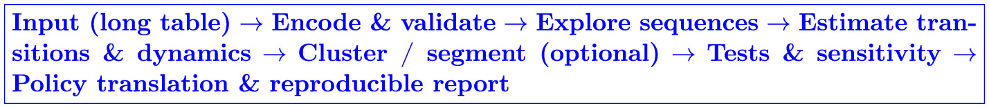
Workflow overview of sequenceRCT. Section 6 instantiates this pipeline on simulated data, while Table 1 summarizes the complete menu of outputs.
For transparency, Table 1 provides a complete summary of the analytic modules and outputs that sequenceRCT can generate. Section 6 presents a representative subset of these outputs to keep the illustration focused on a single decision problem (booster timing).
Table 1
| Module | Outputs (examples) | Decision/reporting use |
|---|---|---|
| Encoding & QC | State definitions; censoring and missingness summaries; participant–time audit trails; checks for impossible transitions | Makes assumptions explicit; supports preregistration and auditing; flags data issues that can distort transition estimates |
| Exploration | Sequence index plots; state-distribution plots over time; arm-by-time contrasts with uncertainty bands | Rapid diagnostics of timing, persistence, and heterogeneity; identifies candidate windows for triage, exit, or booster timing |
| Markov structure | Estimated transition matrices by arm; t-step transitions; expected length of stay; bootstrap intervals | Quantifies when and how people move between states; supports forecasting under alternative schedules |
| Dynamics/complexity | Entropy, turbulence, volatility; run-length and time-since-transition summaries | Detects instability and drift; supports monitoring and sensitivity checks; helps prioritize settings where time-varying policy may matter |
| Clustering/segmentation | Trajectory archetypes (OMA/LCS-based) with stability diagnostics; cluster-wise summaries of transitions and complexity | Enables stratified reporting and exploratory targeting (e.g., different booster thresholds by archetype), with clear caveats about causal validity |
| Arm contrasts & tests | Comparisons of transition kernels, complexity metrics, and cluster membership across arms; negative controls | Supports transparent tests aligned with temporal mechanisms rather than single endline contrasts |
| Causal/policy interfaces (optional) | Export of state histories and derived features as time-varying covariates; weight construction when assignment probabilities are known; off-policy evaluation utilities (e.g., IS/DR) | Connects sequence-defined states to g-method workflows and to safe offline evaluation of candidate policies |
| Policy translation | Decision-maker units (e.g., person-weeks in High, time-to-exit); counterfactual policy vignettes; threshold sensitivity | Converts statistical summaries into actionable trade-offs (timing, triage, exit), including capacity-aware sensitivity analysis |
| Reproducible artifacts | Analysis manifest; saved objects; reproducible tables/figures; session info | Supports replication, preregistration alignment, and audit-ready reporting |
Comprehensive overview of sequenceRCT workflow modules and outputs (beyond the subset illustrated in Section 6).
3.4 Added value relative to existing tools
Established packages such as TraMineR excel at general sequence analysis, but they are not opinionated about RCT-specific tasks. sequenceRCT specializes by centring arm-wise comparisons of transition kernels and expected staying times; offering bootstrap uncertainty as a first-class output for transitions, complexity metrics, and cluster assignments; providing design-phase diagnostics, including state occupancy and overlap or positivity checks, that inform measurement cadence and SMART or MRT exploration; and generating a policy report with figures, tables, and a lightweight checklist that maps estimates to concrete actions. These features aim to reduce the distance between technical analyses and the policy decisions practitioners must make week to week.
3.5 Interfaces to personalisation and reinforcement learning
Because personalisation and sequential decision-making are increasingly common in behavioral public policy, the package exposes simple interfaces for exporting sequence-derived state representations and features, including run-lengths, time since last transition, and volatility windows, to hierarchical ITE models; and for supplying compact, interpretable state spaces and empirical transition kernels to contextual bandits and Q-learning routines, with optional off-policy evaluation hooks (per-decision IS/WIS and doubly robust estimators, with effective sample size and weight diagnostics). This allows researchers to start with descriptive sequence diagnostics and proceed, when appropriate, to policy learning within a coherent state space.
3.6 Reproducibility and reporting
Each analysis run yields a structured object that can be saved and reloaded, a folder of figures and tables keyed to the reporting checklist in Section 5, and a short machine-readable manifest recording the state definitions, cost schemes, bootstrap seeds, and package versions. The documentation includes code templates aligned with the empirical illustration so that readers can reproduce and adapt the full pipeline on their own data with minimal modification.
3.7 Limitations and roadmap
sequenceRCT is research-use software. Current limitations include a focus on first-order transitions, with higher-order memory handled diagnostically rather than modeled by default, and basic missingness options. Planned extensions include support for multi-state survival modules, better integration with seqHMM-type latent-state models, and additional off-policy evaluation estimators for reinforcement learning use cases (including inverse probability weighting and weighted doubly robust variants, with built-in overlap diagnostics).
4 Designing RCTs for temporal inference
4.1 Studying order and staying time requires observing them
This section links the inferential aims introduced in Sections 2 and 2.2 and the software pipeline in Section 3 to concrete design choices that make temporal inference feasible and ethically responsible.
4.2 Measurement cadence
Cadence must resolve the shortest policy-relevant interval, such as weekly relapse. High-frequency observation increases burden and reactivity (Shiffman et al., 2008; Insel, 2017); adaptive cadence, for example denser sampling after a state change, balances cost and sensitivity. The diagnostics in sequenceRCT, including state occupancy and missingness or censoring summaries, are designed to inform these decisions before fielding.
4.3 State construction
Define mutually exclusive and exhaustive states that align with decisions, for example Relapsed mapping to a triage action. Ordinal versus nominal coding affects distance metrics and interpretability (Veltri, 2023). Ensure reliable measurement and pre-register coding rules. The package's encoding module enforces exclusivity and exhaustiveness checks and records definitions in a manifest for reproducibility.
4.4 Adaptive designs
Sequential Multiple Assignment Randomized Trials and Micro-Randomized Trials generate decision-point data (Collins et al., 2014; Boruvka et al., 2018). They pair naturally with sequence outputs to learn escalation or de-escalation policies and to ensure adequate exploration of rarely visited but decision-critical states.
4.5 Ethics
Finer cadence raises privacy concerns and a duty of care if harmful patterns, such as severe relapse, are detected (Sanders et al., 2018). Plans for secure handling, thresholds for alerts, and participant support should be explicit. The reporting checklist in Section 5 includes minimum transparency standards for these issues.
5 A decision framework and reporting checklist
Having established why temporal structure matters, how sequence methods relate to alternatives, and how the workflow is implemented in practice, we now connect analytical outputs to policy decisions. Table 2 maps common policy questions to methods, design implications, and concrete outputs. The aim is not to be exhaustive but to make explicit which tool answers which decision, under what measurement conditions, and with which uncertainties.
Table 2
| Policy question | Suitable methods | Design and measurement | Actionable output |
|---|---|---|---|
| When do relapse windows occur? | Sequence plots; Markov transitions; multi-state hazards | Weekly or daily states; relapse definition | Risk windows; booster schedule points |
| Who needs escalation to intensive support? | Sequence clustering; HMM classes; hazard-based risk scores | Minimal cadence for timely classification | Triage rule: escalate if P(Medium → Low)>τ |
| Does treatment increase staying time in desirable states? | Markov Pii; multi-state expected length of stay | Balance observation across phases | Target: ΔLOS relative to control |
| Which sequence of nudges works best? | SMART or MRT; dynamic treatment regimes | Multiple decision points | Adaptive policy: context to action map |
| Are effects transient or sticky? | State distributions; change-point or TVEM | Sufficient follow-up | Re-nudge cadence; sunset criteria |
| How should we personalize decisions over time? | Sequence features plus hierarchical ITE models; contextual bandits | Individual state histories; context features | Per-person thresholds; escalation or exit rules |
From policy question to method, design, and actionable output.
In applications, we recommend reporting at least one non-sequence comparator, such as a multi-state hazard model, alongside sequence analyses to assess the robustness of staying-time and transition conclusions.
5.1 Reporting checklist (minimum transparency)
States: define and justify states; ordinal versus nominal. Cadence: justify frequency versus burden; describe missingness and imputation or weighting. Assumptions: declare Markov or other assumptions; test for higher-order memory. Causal identification: state whether decision points are randomized; if not, specify the g-method/propensity model, positivity checks, and sensitivity analyses. State sufficiency and partial observability: justify whether sequence states are intended as causal states or predictive proxies; if partial observability is likely, discuss POMDP/belief-state approaches. Distances and costs: if OMA or LCS, justify the cost scheme and report sensitivity. Comparators: include at least one alternative analysis, such as multi-state hazards, for robustness. Uncertainty: provide bootstrap or standard errors for transitions, complexity, and cluster stability. Action mapping: show how estimates trigger policy actions, including thresholds and timing rules.1
5.2 Practitioner's summary
Define discrete states that match actions; measure often enough to resolve relapse windows; report state-specific transitions with uncertainty; map transitions to rules for when to boost, escalate, or exit; pre-register thresholds; include at least one non-sequence comparator; evaluate value in decision units such as person-weeks in High and cost per added week; and audit subgroup equity.
6 Empirical illustration (simulated): interpretation and decision use
6.1 Purpose
The empirical component is an illustration, not a claim of external validity. Its role in the paper is to show, end to end, how the sequence-analytic workflow produces interpretable temporal evidence and how those estimates feed the decision framework in Section 5. All analyses in this section were generated with the sequenceRCT pipeline. The figures shown below are intentionally selective; Table 1 summarizes the full set of package outputs and diagnostics that can be produced from the same analysis object.
6.2 Data-generating process
We simulate weekly states {Low, Medium, High} over T = 10 for parallel treatment and control arms. Individuals vary in age (Normal(μ = 35, σ = 10)), prior engagement (Beta, right-skewed), and responsiveness (log-normal). The treatment increases upward transition probabilities, Low to Medium and Medium to High, and exhibits fade-out governed by e−0.2t. Attrition is set at 15% and is uniformly distributed over time. This specification creates realistic ingredients for policy analysis while keeping the state space concise enough to visualize and to map onto clear actions. Full implementation details, including seeds and estimation options, are described in Appendix A.
6.3 Sequence outputs
The first diagnostic step examines individual trajectories and their aggregation. The sequence index plots and state-distribution plots in Figures 2, 3 show two features consistent with a treatment that primarily facilitates upward moves. First, relative to control, the treatment arm exhibits more frequent visits to High and less stagnation in Low. Second, complexity measures, including entropy, turbulence, and volatility, are higher in treatment, reflecting a greater amount of movement across states; whether such dynamism is desirable depends on where transitions terminate.
Figure 2
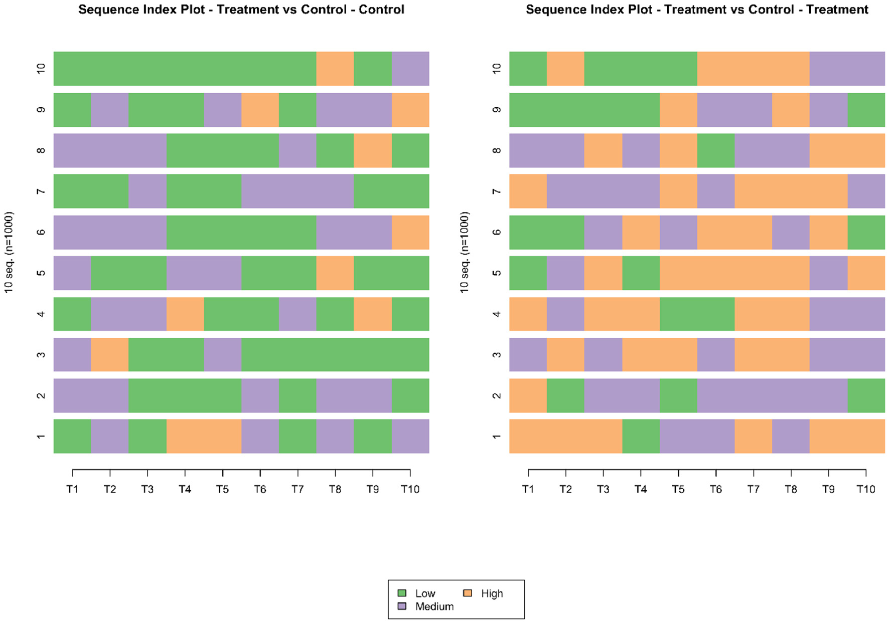
Sequence index plots for treatment and control. Each row is a participant from t = 1 to t = 10 with states low, medium, or high.
Figure 3
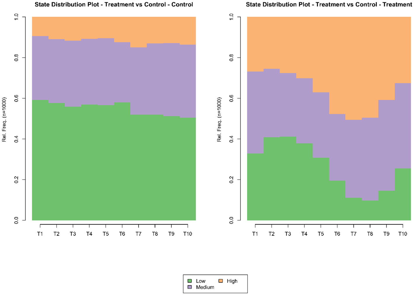
State-distribution plots over time. Bands show the share in each state.
6.4 Transitions that drive decisions
Estimated one-step transition matrices (Tables 3, 4) quantify how the intervention reshapes movement among states. Three patterns are decision relevant. Stability of improvement: in treatment, P(High → High) is larger than in control, implying longer staying time once improved. Climbing the ladder: P(Medium → High) is higher under treatment, supporting boosters aimed at moderately engaged participants. Direct jumps: the treatment arm displays a larger probability of Low to High transitions than control, suggesting a subgroup of sharp responders and motivating further investigation; differentiated booster policies would require confirmation in a design that randomizes booster rules (e.g., SMART/MRT) rather than being inferred causally from post-baseline subtypes alone as visualized in Figure 4.
Table 3
| From/To | High | Medium | Low |
|---|---|---|---|
| High | 0.391 | 0.373 | 0.236 |
| Medium | 0.382 | 0.364 | 0.254 |
| Low | 0.360 | 0.351 | 0.289 |
Transition probabilities, treatment.
Table 4
| From/To | High | Medium | Low |
|---|---|---|---|
| High | 0.116 | 0.339 | 0.545 |
| Medium | 0.128 | 0.332 | 0.539 |
| Low | 0.121 | 0.330 | 0.549 |
Transition probabilities, control.
Figure 4
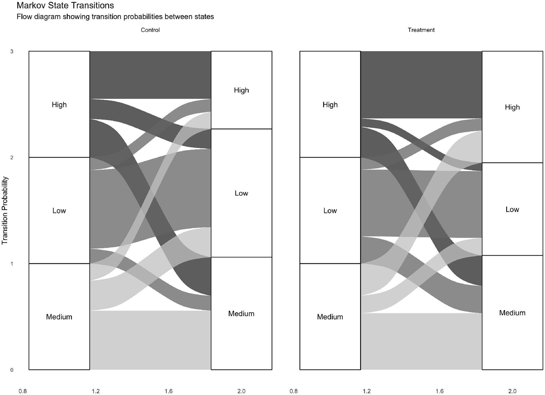
Markov transition visualizations for both groups. Chords illustrate relative one-step flows; thickness is proportional to estimated transition probability.
6.5 Comparator analysis
As a robustness check, we also fit a three-state continuous-time multi-state model with piecewise-constant hazards at weekly cut-points. The hazard-based expected length-of-stay contrasts align with the Markov summaries: treatment is associated with longer stay in High and higher hazard of Medium to High transitions; specification and estimation details are given in Appendix C. Code to reproduce this comparator analysis is provided at the OSF link in the Declarations.
These inferences follow from the row-stochastic structure of the estimated matrices, bolstered by the visual evidence that the distribution of states shifts in ways consistent with the transition contrasts. In the workflow, sequenceRCT reports nonparametric bootstrap intervals for transition probabilities and for derived quantities such as expected length of stay, so that decisions can be matched with uncertainty.
Robustness, ablations, and negative controls. To clarify what features of the illustration are structural and which are artifacts of assumptions, we report three diagnostic variants implemented in the supplement. A no-effect placebo removes the treatment modification to the transition kernel; arm differences in transitions and complexity then collapse toward equality. A time-invariant effect eliminates fade-out; the wear-off signatures in the state-distribution plots disappear. Finally, distance-scheme sensitivity varies OMA or LCS costs in the clustering stage; the substantive cluster distinctions and the arm contrasts remain directionally stable.
Counterfactual policy vignette, booster timing. To demonstrate how transition estimates translate into resourced decisions, consider a simple rule: deliver a booster at t+1 if the predicted risk of slippage from High exceeds a threshold, Pt(High → {Medium, Low})>τ3, or if the risk of deterioration from Medium is high, Pt(Medium → Low)>τ1. In this vignette the booster is targeted rather than universal: it is delivered only to individuals who meet the rule at a scheduled decision point (weekly here), and otherwise withheld. The thresholds (τ1, τ3) are chosen to reflect capacity, budget, or equity constraints (e.g., treating the top x% highest-risk person-weeks), so we report sensitivity over (τ1, τ3) rather than privileging a single tuned value. A concrete real-world mapping is a reminder programme (e.g., SMS/email/app outreach) where a “booster” corresponds to an additional message or outreach triggered when the predicted probability of next-week deterioration exceeds a policy threshold. Using the estimated matrices, we project expected total weeks in High over T = 10 under no boosters and under this rule. The incremental difference can be reported as additional person-weeks in High per 1000 participants; combined with unit booster costs, it yields a cost per extra week in High. Sensitivity analyses over (τ1, τ3) trace the precision-recall trade-off.
Segmentation and differentiated targeting. The temporal outputs above can be combined with segmentation to propose differentiated interventions. After constructing trajectory archetypes via sequence clustering (e.g., OMA/LCS-based), sequenceRCT can produce cluster-wise transition summaries and evaluate stratified policies, such as cluster-specific thresholds or different actions (booster, triage, exit) by archetype. Table 5 gives a decision-focused example of how archetypes can be translated into differentiated actions. Importantly, when archetypes are learned from post-baseline behavior, this is a predictive segmentation tool; causal validity of cluster-specific allocation rules should be established in designs that randomize the allocation rule (e.g., SMART/MRT) or by defining archetypes from pre-treatment/run-in data, as discussed in Section 7.
Table 5
| Archetype (example) | Typical temporal pattern | Example decision implication |
|---|---|---|
| Stable Low/sustained adherence | Long stays in Low with rare upward transitions | “Exit” or minimal-touch maintenance; avoid unnecessary boosters |
| Volatile/relapse-prone | Frequent Medium↔High movement; short run-lengths | Lower booster threshold or earlier triggering; monitor drift and support needs |
| Persistent High / stuck | High self-loop; low probability of improvement absent escalation | Triage to higher-intensity support or alternative pathway; consider equity and capacity constraints |
Illustrative examples of how trajectory archetypes can inform differentiated decisions (conceptual; archetype labels are descriptive).
7 Personalized interventions and individual treatment effects
Personalized, adaptive interventions tailor content, timing, and intensity to a person's evolving context. Such tailoring promises better outcomes, but it complicates identification and estimation of individual treatment effects. Three interrelated difficulties are especially salient in policy settings, and each links back to the need for explicit sequence representations.
Selective exposure and nonstationarity. As interventions adapt, exposure depends on prior states and outcomes. This induces time-varying confounding by indication and creates nonstationarity: the same person encounters different decision contexts over time, and the mapping from context to action may drift. By organizing histories into discrete, decision-relevant states, sequence methods render the sources of adaptivity explicit and provide the conditioning sets needed for causal estimators.
Data fragmentation at the individual level. Personalisation pushes inference toward the individual, where panels are short, noisy, and state-dependent. Pooling across people is hazardous when individuals traverse different regions of the state space. Sequence-based stratification mitigates this by grouping individuals with similar path topologies, enabling partial pooling within empirically coherent archetypes while avoiding unjustified borrowing across archetypes.
Heterogeneity across positions in a trajectory. Effects are not only person specific but also state specific. Estimating effects on transition probabilities, for example ΔP(Medium → High), aligns directly with the next-move logic of Section 5.
How sequence analysis helps. The approach operationalises these ideas in four ways. First, by conditioning on current state and recent run-lengths, one estimates position-specific effects that align with decision points. Second, clustering sequences yields archetypes within which hierarchical models can stabilize per-person estimates without assuming global homogeneity. Third, dwell times, volatility, entropy, and time since last transition serve as low-dimensional summaries for hierarchical shrinkage in short panels. Fourth, state-distribution plots expose lack of support in parts of the state space, warning against extrapolation and guiding exploration in SMART or MRT designs. In sequenceRCT, these summaries and diagnostics are available as standard outputs.
Methodological notes. When exposure is adaptive, g-methods and dynamic treatment-regime estimators provide identification under explicit assumptions; sequence-derived states and features enter these models as time-varying covariates. Specifically, the g-formula (g-computation), marginal structural models estimated via inverse probability weights, and structural nested models provide standard routes to estimating dynamic treatment effects when treatment depends on evolving histories and time-varying confounding is present. Appendix A gives a concise formulaic example using the state history S1:t to construct time-varying covariates Lt and to estimate state-specific contrasts such as “receive At = 1 versus At = 0 under St = s”. For N-of-1 settings, Bayesian hierarchical models with sequence summaries allow partial pooling across similar trajectories while respecting person-specific dynamics. Principal stratification can be recast using early trajectory segments, such as early responders, as pre-treatment strata.
Prediction versus causation in trajectory subtypes. Trajectory clusters or “responder subtypes” identified from realized sequences are often valuable descriptively and for support diagnostics, but they do not automatically define causal subgroups: if clustering uses post-baseline behavior, cluster membership may be affected by treatment and can induce post-treatment selection bias. These subtypes can be used for stratified reporting, hypothesis generation, or as effect modifiers in confirmatory designs; using them for future personalized allocation is a predictive modeling step whose causal validity must be established in new randomized studies (e.g., SMART/MRTs that randomize the allocation rule) or under strong additional assumptions.
8 Reinforcement learning meets sequence analysis
Reinforcement learning formalizes sequential decision-making under uncertainty and resource constraints. In many applications, such as deciding whom to nudge, when to boost, and when to escalate, reinforcement learning complements the statistical tools discussed above by optimizing policies rather than only estimating effects. Sequence analysis is useful at three stages: representation, learning, and evaluation or safety. Table 6 summarizes how sequence outputs map onto reinforcement learning components.
Table 6
| Sequence output | RL component | Use |
|---|---|---|
| State taxonomy and dwell or run-lengths | State representation | Markov aggregation; eligibility traces; recency features |
| Transition matrix | Environment kernel (sim/offline) | Policy stress tests; sensitivity to drift |
| Volatility or entropy | Safety monitor | Detect unstable regimes; trigger conservative actions |
| Trajectory clusters | Policy segmentation | Learn segment-specific policies; partial pooling for value estimates |
| Relapse windows | Reward shaping or constraints | Penalize actions near high-risk windows or pre-empt with boosters |
How sequence outputs map onto reinforcement learning components.
Representation. Reinforcement learning depends on a state representation that renders the future conditionally independent of the past given the present. Sequence analysis supports this step by defining discrete decision states that preserve predictive information, by supplying feature libraries for function approximation, including complexity measures, time since last transition, and n-gram encodings, and by estimating empirical transition kernels that can seed simulators and stress tests before online exploration.
Causal sufficiency, confounding, and partial observability. In reinforcement learning, the Markov requirement is ultimately interventional: a state used for policy learning should be sufficient for the transition and reward distributions under intervention. When states are constructed from observed behavioral sequences, they are typically proxies for a richer latent causal state that may include unmeasured drivers (e.g., motivation, emotions, shocks, external events). In such cases, the transition kernel estimated from logged data, P(St+1∣St, At), need not equal the causal kernel P(St+1∣St, do(At)), i.e., P(s′∣s, a)≠P(s′∣do(a), s) under unobserved confounding or confounding-by-indication. This distinction matters because value estimation and policy improvement can be biased when actions are preferentially applied in high-risk or high-motivation moments not fully captured by the observed state. Designs that randomize actions at decision points (e.g., MRT/SMART) mitigate this concern by construction; in observational or clinician-driven implementations, sequence-defined states should be paired with g-methods/propensity models and sensitivity analysis rather than treated as causally sufficient.
Learning. Different formalisms align with different intervention logics. In micro-randomized trials, contextual bandits approximate one-step decisions. When actions have multi-step consequences, finite-state Markov decision processes and Q-learning are appropriate, with sequence-derived states improving interpretability and sample efficiency. If key determinants are latent, partially observed models are a principled extension; sequence clustering or hidden Markov models can be used to construct tractable belief states. Formally, this corresponds to a partially observable Markov decision process (POMDP), in which an unobserved latent state Zt evolves Markovianly and the analyst observes Ot (here, the sequence label) through an emission model. The relevant Markovian representation is then the belief state bt(z) = P(Zt = z∣O1:t, A1:t−1). Hidden Markov models provide a tractable route to estimating Zt and filtering bt; sequence clustering can be viewed as a coarse state abstraction or regime discovery tool, but it does not by itself provide belief updates unless embedded in a state-space model. In all cases, the state abstractions provided by the software link descriptive diagnostics to policy learning.
Model-based versus model-free learning (and feasibility). Using the estimated transition matrix as a simulator kernel is a model-based approach: it supports stress testing, interpretability, and sample-efficient planning on compact state spaces, but it inherits bias from state misspecification, partial observability, and sparse state–action coverage. Model-free approaches (e.g., tabular or fitted Q-learning, policy-gradient methods with sequence-derived features) avoid explicit transition modeling and can exploit richer function approximation, but typically require larger datasets and can be unstable offline when the target policy extrapolates beyond the support of logged actions. Computationally, discrete model-based kernels scale with the number of state–action cells: with states and actions, estimating transitions involves O(mK(K−1)) parameters and becomes unreliable when many cells are rarely visited. For small policy RCTs, this motivates deliberately coarse, decision-relevant state taxonomies, shrinkage/smoothing for transition estimates, and explicit reporting of state–action support.
Evaluation and safety. Offline evaluation is critical where exploration is costly or ethically constrained. Importance sampling and doubly robust estimators leverage logged data to estimate the value of a new policy without deploying it; In micro-randomized settings, the logging policy is known by design (randomization probabilities), simplifying weight construction and strengthening overlap; in observational or clinician-driven allocation, propensities must be estimated and positivity becomes a primary diagnostic. In sequenceRCT, OPE takes the sequence-derived (St, At) histories (and rewards or terminal outcomes) together with known or estimated logging probabilities and returns per-decision IS/WIS and doubly robust value estimates, effective sample size, weight diagnostics, and bootstrap uncertainty. sequence-based states improve overlap and reduce variance by aligning evaluation with true decision contexts. Safety requires monitoring for nonstationarity and drift: volatility and entropy profiles flag regimes where small policy changes can have outsized downstream effects. Resource and equity constraints can be imposed during learning and audited post hoc using subgroup-specific transition and staying-time summaries already computed in the sequence workflow.
Checklist for sequence-informed reinforcement learning. State design: define states from sequences and test Markov adequacy with predictive checks. Exploration plan: use MRT or SMART to ensure coverage of key states; cap exploration in unsafe regimes. Off-policy evaluation: report importance weights, effective sample size, and doubly robust estimates with confidence intervals, alongside overlap/positivity diagnostics (state–action visitation counts and weight distributions) to document support for the target policy. Drift monitoring: track transition kernels and volatility over time; adapt policies if drift is detected. Equity constraints: evaluate value by subgroup; enforce fairness or resource constraints during learning. Interpretability: prefer state spaces whose semantics support policy communication and governance.
9 Limitations and path to empirical validation
The empirical component is synthetic and intended for interpretation and decision mapping, not external validity. The framework should be validated on existing behavioral datasets. A practical path is to define states with domain experts; encode sequences and estimate transitions with uncertainty; run at least one alternative analysis such as multi-state hazards; implement the booster vignette using observed transitions; for personalized policies, run contextual bandit or Q-learning analyses with sequence-derived state representations and report off-policy evaluation with overlap diagnostics; and report performance, resource, and equity impacts. We recommend preregistering state definitions, cadence, thresholds, and robustness checks.
Internal validity and identification. The illustration clarifies interpretation but does not establish causal effects in a specific domain. Even with randomization, adaptive exposure complicates identification. Estimands that are meaningful for decisions, such as ΔP(Medium → High) by arm, require careful conditioning on states and documented sequential ignorability. Where exposure depends on evolving histories, g-methods and dynamic treatment-regime estimators should be used alongside the sequence workflow to guard against time-varying confounding.
Measurement and state construction. State definitions are consequential. Discretisation that is too coarse hides relapse windows; discretisation that is too fine yields sparse states and unstable transitions. Misclassification can bias transition estimates and, in turn, decision rules. We therefore recommend a pre-analysis protocol that includes expert elicitation of states tied to concrete actions, sensitivity to alternative taxonomies, and robustness checks that re-estimate transitions under jittered labels and alternative cadence. The sequenceRCT encoding module records these choices in a run manifest and provides overlap diagnostics.
Model assumptions and uncertainty. The main text reports first-order transitions; higher-order memory may matter in some behaviors. The package includes diagnostics but defaults to first order for interpretability. Uncertainty is addressed via nonparametric bootstrapping over individuals; where cluster-level dependence or interference are plausible, block bootstrap or design-aware resampling should be used. Complexity measures are sensitive to the observation window; reporting them with time normalization and uncertainty bands is essential.
Nonstationarity and drift. Transition kernels may drift over time, violating the stationarity assumed by simple Markov summaries. Monitoring drift via rolling-window estimates of , comparing kernels with distance measures, and inspecting volatility and entropy trends can alert to regime shifts. Decision rules derived from early data should therefore be audited prospectively, and guardrails adopted when drift is detected. As a coarse-graining sensitivity, re-estimating with a binary state partition, for example High versus Not-High, should yield consistent qualitative conclusions if policy value derives from stabilizing High.
Generalizability and transportability. Findings from one context may not transport to another due to differences in state occupancy, exposure patterns, or institutional frictions. Transport analyses should therefore report how much of the target population's state distribution lies outside the support of the source study, whether key transitions are rare or absent, and the sensitivity of policy value under counterfactual reweighting.
Computational and software constraints. Pairwise distances for clustering scale quadratically with sample size, and heavy bootstrap resampling increases compute time. sequenceRCT provides caching and selective recomputation, but large deployments may require subsampling or approximate distances. The package currently prioritizes first-order transitions; explicit multi-state hazard modules and HMM interfaces are on the roadmap.
Ethics, equity, and governance. Finer cadence and responsive policies raise privacy and duty-of-care considerations. Decision rules that improve overall staying time in desirable states may still widen subgroup disparities. We recommend reporting equity impacts as differences in expected weeks in High across protected groups, with bootstrap uncertainty, and adopting fairness-constrained policies if trade-offs are material. All decision thresholds and monitoring plans should be preregistered or, at minimum, logged.
A multi-phase validation agenda. Phase I, stress testing on synthetic regimes: include higher-order memory, latent regimes, heavy missingness and MNAR scenarios, and structured nonstationarity. Evaluate calibration of transition probabilities, coverage of bootstrap intervals, stability of cluster archetypes across cost schemes, and robustness of policy value under the booster vignette to misspecification. Phase II, retrospective re-analysis of completed trials: apply the pipeline to multiple datasets; compare with multi-state survival; evaluate out-of-sample prediction of next-state transitions, agreement between Markov and hazard-based staying-time estimates, and value of historical booster timing rules under off-policy evaluation. A particularly tractable class of real-world datasets for Phase II are behavioral megastudies that test many interventions on a common, objectively measured outcome in the same population (e.g., Milkman et al., 2021). When such datasets include repeated opportunities or repeated behavioral measurements (e.g., weekly engagement, return visits, adherence windows), they map naturally into sequence states: define a small decision-relevant state space, align the time index, encode sequences with censoring, estimate transition kernels by arm, and translate differences into decision-maker units (person-weeks in High, time-to-exit). Practical barriers include limited within-person temporal granularity in some trials, data access/privacy constraints, and potential interference or spillovers; these considerations inform state definitions, reporting, and the choice of causal estimators. Phase III, prospective augmentation of new trials: embed sequence endpoints, cadence diagnostics, and prespecified booster rules in new designs. Primary outcomes should include person-weeks in High, with transition-based secondary endpoints. Where feasible, evaluate personalized policies via contextual bandits or Q-learning using sequence-derived states, and report off-policy evaluation with overlap diagnostics. Phase IV, operational piloting and monitoring: deploy decision rules with conservative thresholds initially, monitor drift in and volatility or entropy, and implement equity audits. Report resource implications and policy value in decision-maker units, such as cost per additional person-week in High.
Success criteria and reporting. Across phases, report predictive accuracy and calibration for next-state models, uncertainty coverage for transitions and staying times, policy value and its uncertainty under off-policy evaluation, resource use and sensitivity to thresholds, and subgroup equity impacts. These criteria align with the reporting checklist in Section 5 and are implemented as outputs in sequenceRCT. Figures 2, 3 and Tables 3, 4 illustrate the minimal objects that make this pathway operational.
10 Conclusion
Temporal questions are decision questions: when to boost, whom to escalate, and when to stop. Sequence-informed tools are most valuable when they change those decisions. Under personalisation, where effects become difficult to detect due to adaptivity and selective exposure, sequence methods provide state-specific contrasts, trajectory stratification, and diagnostics that keep inference honest. For learning adaptive policies, reinforcement learning and sequence analysis are natural partners: the former optimizes actions; the latter supplies the state abstractions, kernels, and stability checks that make optimisation interpretable and safe. By positioning sequence methods alongside alternatives, clarifying design requirements, and making outputs actionable through rules and checklists, we aim to normalize time-sensitive, personalized analyses in RCTs without unnecessary technical burden. Full derivations and software details are in the appendices; the main text centers implications for policy.
What the paper offers. The contribution is pragmatic. First, we show how and when sequence methods complement, rather than replace, standard longitudinal analyses. Second, we translate sequence outputs into concrete actions via a decision framework and reporting checklist. Third, we deliver a software layer, sequenceRCT, that turns the workflow into reproducible artifacts suitable for preregistration, auditing, and iterative improvement.
What the illustration teaches. The synthetic example demonstrates how differences in transition structure, not only cross-sectional means, underpin policy value: higher P(High → High) and P(Medium → High) in the treatment arm imply longer staying times and better prospects for well-timed boosters. The same outputs enable budgeting in familiar units, such as person-weeks in desirable states.
What remains to be shown. The agenda in Section 9 lays out a path to empirical validation that goes beyond demonstration: retrospective re-analysis with alternative models; prospective embedding in new trials; and operational pilots with monitoring, drift detection, and equity audits. Success requires collaboration between methodologists, domain experts, and practitioners because state definitions and cadence choices must be negotiated in light of ethics, burden, and feasibility.
A forward look. Two extensions are likely to matter for the field. First, deeper integration with multi-state survival and hidden Markov models can reconcile hazard-based interpretations with sequence-level communication. Second, the coupling of sequence representations with reinforcement learning, especially in constrained, fairness-aware settings, can move programmes from static interventions to responsive systems that learn safely over time. In sum, treating trajectories as first-class data objects illuminates how change unfolds and when to act.
Statements
Data availability statement
The simulated datasets and analysis code presented in this study are available in the OSF repository: https://osf.io/rtx8k. The R package sequenceRCT, including documentation and code templates, is available at the same repository and is released under the MIT license for research use.
Author contributions
GV: Conceptualization, Data curation, Formal analysis, Funding acquisition, Investigation, Methodology, Project administration, Resources, Software, Supervision, Validation, Visualization, Writing – original draft, Writing – review & editing.
Funding
The author(s) declared that financial support was not received for this work and/or its publication.
Conflict of interest
The author(s) declared that this work was conducted in the absence of any commercial or financial relationships that could be construed as a potential conflict of interest.
Generative AI statement
The author(s) declared that generative AI was not used in the creation of this manuscript.
Any alternative text (alt text) provided alongside figures in this article has been generated by Frontiers with the support of artificial intelligence and reasonable efforts have been made to ensure accuracy, including review by the authors wherever possible. If you identify any issues, please contact us.
Publisher’s note
All claims expressed in this article are solely those of the authors and do not necessarily represent those of their affiliated organizations, or those of the publisher, the editors and the reviewers. Any product that may be evaluated in this article, or claim that may be made by its manufacturer, is not guaranteed or endorsed by the publisher.
Supplementary material
The Supplementary Material for this article can be found online at: https://www.frontiersin.org/articles/10.3389/frbhe.2026.1684887/full#supplementary-material
Footnotes
1.^A fuller template with examples is provided in the OSF materials.
References
1
Abbott A. (2000). Sequence analysis: new methods for old ideas. Annu. Rev. Sociol. 26, 93–113. doi: 10.1146/annurev.soc.21.1.93
2
Abbott A. Forrest J. (1986). Methods of comparison in social science research. Annu. Rev. Sociol. 12, 419–437.
3
Anderson T. W. (2017). Hidden Markov Models for Time Series: an Introduction Using R. London: Chapman and Hall/CRC.
4
Bergroth L. Hakonen H. Raita T. (2000). “A survey of longest common subsequence algorithms,” in Proceedings of the 7th International Symposium on String Processing and Information Retrieval (SPIRE 2000) (A Coruna: IEEE Computer Society), 3948. doi: 10.1109/SPIRE.2000.878178
5
Boruvka A. Almirall D. Witkiewitz K. Murphy S. A. (2018). Assessing time-varying causal effect moderation in mobile health. J. Am. Statist. Assoc. 113, 1112–1121. doi: 10.1080/01621459.2017.1305274
6
Buyalskaya A. Ho H. Milkman K. L. Li X. Duckworth A. L. Camerer C. (2023). What can machine learning teach us about habit formation? Evidence from exercise and hygiene. Proc. Nat. Acad. Sci. 120:e2216115120. doi: 10.1073/pnas.2216115120
7
Charness G. Gneezy U. (2009). Incentives to exercise. Econometrica77, 909–931. doi: 10.3982/ECTA7416
8
Collins L. M. Kugler K. C. Gwadz M. V. (2014). Optimizing adaptive interventions in behavioral health: Intersecting the experimental design of smart and the future of prevention science. Clinical Trials11, 705–715.
9
Elzinga C. H. Liefbroer A. C. (2010). Sequence turbulence in social processes. Sociol. Methods Res. 38, 442–473. doi: 10.1177/0049124109357535
10
Frey E. Rogers T. (2014). Persistence: How treatment effects persist after interventions stop. Policy Insights Behav. Brain Sci. 1, 172–179. doi: 10.1177/2372732214550405
11
Gabadinho A. Ritschard G. Müller N. S. Studer M. (2011). Analyzing and visualizing state sequences in R with TraMineR. J. Statist. Softw. 40, 1–37. doi: 10.18637/jss.v040.i04
12
Insel T. R. (2017). Digital phenotyping: Technology for a new science of behavior. JAMA318, 1215–1216. doi: 10.1001/jama.2017.11295
13
Lesnard L. (2010). Setting cost in optimal matching to uncover contemporaneous socio-temporal patterns. Sociol. Methods Res. 38, 389–419. doi: 10.1177/0049124110362526
14
Maier M. Bartoš F. Stanley T. D. Shanks D. R. Harris A. J. L. Wagenmakers E.-J. (2022). No evidence for nudging after adjusting for publication bias. Proc. Nat. Acad. Sci. 119:e2200300119. doi: 10.1073/pnas.2200300119
15
Milkman K. L. Gromet D. Ho H. Kay J. S. Lee T. W. Pandiloski P. Park Y. Rai A. Bazerman M. Beshears J. et al . (2021). Megastudies improve the impact of applied behavioural science. Nature600, 478–483. doi: 10.1038/s41586-021-04128-4
16
Norris J. R. (1998). Markov Chains, volume 2. Cambridge: Cambridge University Press.
17
Prochaska J. O. Velicer W. F. (1997). The transtheoretical model of health behavior change. Am. J. Health Prom. 12, 38–48. doi: 10.4278/0890-1171-12.1.38
18
Ross S. M. (2014). Introduction to Probability Models. London: Academic Press.
19
Sanders M. Snijders V. Hallsworth M. (2018). Behavioural science and policy: where are we now and where are we going?Behav. Public Policy2, 144–167. doi: 10.1017/bpp.2018.17
20
Sankoff D. Kruskal J. B. (1983). Time Warps, String Edits, and Macromolecules: The Theory and Practice of Sequence Comparison. Reading: Addison-Wesley Publication.
21
Shannon C. E. (1948). A mathematical theory of communication. Bell System Techn. J. 27, 379–423. doi: 10.1002/j.1538-7305.1948.tb01338.x
22
Shiffman S. Stone A. A. Hufford M. R. (2008). Ecological momentary assessment. Annu. Rev. Clini. Psychol. 4, 1–32. doi: 10.1146/annurev.clinpsy.3.022806.091415
23
Stewart W. J. (2009). Probability, Markov Chains, Queues, and Simulation: the Mathematical Basis of Performance Modeling. Princeton, NJ: Princeton University Press.
24
Studer M. (2013). A weighted cluster library for sequence analysis. J. Statist. Softw. 54, 1–26. doi: 10.18637/jss.v054.i01
25
Studer M. Ritschard G. (2016). Analyzing inter-sequences similarities with probabilistic suffix trees: an application to sociodemographic sequences. Sociol. Methods Res. 45, 677–710.
26
Veltri G. A. (2023). Designing Online Experiments for the Social Sciences. London: SAGE Publications Ltd.
27
Ward Jr J. H. (1963). Hierarchical grouping to optimize an objective function. J. Am. Statist. Assoc. 58, 236–244. doi: 10.1080/01621459.1963.10500845
Summary
Keywords
behavioral RCTs, Markov modeling, personalization, reinforcement learning, sequence methods, time-sensitive analysis
Citation
Veltri GA (2026) Time-sensitive RCTs in behavioral public policy: a pragmatic framework using sequence methods, personalization, and reinforcement learning. Front. Behav. Econ. 5:1684887. doi: 10.3389/frbhe.2026.1684887
Received
13 August 2025
Revised
14 January 2026
Accepted
15 January 2026
Published
11 February 2026
Volume
5 - 2026
Edited by
Ximeng Fang, University of Oxford, United Kingdom
Reviewed by
Anastasia Buyalskaya, HEC Paris, France
Ruth Schmidt, Illinois Institute of Technology, United States
Cong Jiang, Harvard University, United States
Updates
Copyright
© 2026 Veltri.
This is an open-access article distributed under the terms of the Creative Commons Attribution License (CC BY). The use, distribution or reproduction in other forums is permitted, provided the original author(s) and the copyright owner(s) are credited and that the original publication in this journal is cited, in accordance with accepted academic practice. No use, distribution or reproduction is permitted which does not comply with these terms.
*Correspondence: Giuseppe Alessandro Veltri, gaveltri@nus.edu.sg
Disclaimer
All claims expressed in this article are solely those of the authors and do not necessarily represent those of their affiliated organizations, or those of the publisher, the editors and the reviewers. Any product that may be evaluated in this article or claim that may be made by its manufacturer is not guaranteed or endorsed by the publisher.