 Andreas Palmtag
 Johannes Rousselli
 Henning Gröschl
- Fluid Process Engineering (AVT.FVT), RWTH Aachen University, Aachen, Germany
Accurate models for pulsed sieve tray extraction columns (PSEs) depend on the correct prediction of the drop diameter to estimate extractive mass transfer across the phase boundary. Phenomenologically, the drop diameter is determined by a balance of drop breakage and coalescence. While for most industrial solvent systems, coalescence plays a minor role; breakage is mostly the dominant phenomenon determining the drop diameter. However, most modeling approaches for drop breakage in PSEs are characterized by a trade-off between a broad validity range and good prediction accuracy. To overcome this limitation, we developed a hybrid breakage model for drop breakage in PSEs in which a physical-empirical model basis is enhanced by data-driven parameter estimator models (PEMs). The hybrid model is based on a revised form of Garthe’s breakage model, for which we developed a linear PEM for the model parameters and two data-driven PEMs for
1 Introduction
Pulsed sieve tray extraction columns (PSE) are one of the most common process equipment for industrial extraction, having found application in chemical and hydrometallurgical processes, in biotechnology, and particularly in nuclear fuel reprocessing (Lo et al., 1983; Schügerl, 1994; Gameiro et al., 2010). The numerous industrial applications have motivated intensive research on PSE, including experimental studies and the development of column models with various degrees of rigor. Particularly, the wish to limit the number of preliminary column experiments on a technical scale induced the development of models that correctly depict fluid dynamics and mass transfer over several scales. A promising approach for this purpose is based on population balance models (PBMs), which track the evolution of the drop swarm along the column height by accounting for key phenomena such as drop sedimentation and mass transfer by physical-empirical sub-models (Goedecke, 2006; Weber et al., 2019). The accuracy of PBMs highly depends on the correct prediction of the drop diameter, which is crucial for accurate modeling of fluid dynamics and mass transfer in extraction columns (Hlawitschka et al., 2020; Weber and Jupke, 2020). Phenomenologically, the drop diameter is mainly determined by a balance of drop breakage and coalescence phenomena. Commonly, drop breakage is considered dominant since many industrial processes are characterized by significant coalescence inhibition, e.g., due to mass transfer and/or impurities (Henschke, 2003). Consequently, considerable research was conducted to investigate, model, and predict the drop breakage behavior in PSEs.
Most studies on drop breakage behavior are based on single-drop investigations in lab-scale devices to limit the experimental effort. A sketch of a single-drop cell is shown in Figure 1. The cell consists of a single compartment between two sieve trays, a pulsation unit, and a periphery to insert and remove single-drops into/from the cell. The setup in Figure 1 allows the investigation of organic drops (inserted at the bottom) submerged in an aqueous continuous phase. Within the single-drop experiments, the breakage behavior is commonly quantified based on the breakage probability
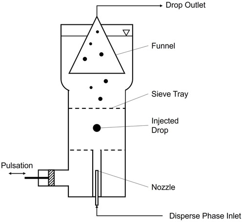
FIGURE 1. Single-drop cell for investigating drop breakage on sieve trays.
Based on the experimental investigations, several modeling approaches for either of the breakage properties
with
Where
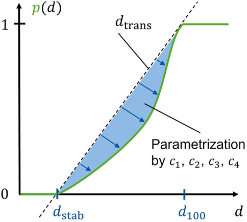
FIGURE 2. Qualitative representation of Garthe’s breakage model.
For sieve trays, Garthe provides eight parameter sets that account for four solvent systems toluene/acetone/water, butyl acetate/acetone/water, toluene/water, butyl acetate/water (abbreviated by TWA, BWA, TW, BW) and two sieve tray orifice diameters (
In the two empirical models by Haverland and Garthe, the prediction of the breakage probability consists of a single mathematical expression, wherein
with
In the final validation of his model, Gourdon showed that Eq 1–6 correctly depicts the trend of the breakage probability over a wide range of operating conditions for the solvent systems TW and TWA despite some considerable deviations for single data sets.
In contrast to pursuing a single correlation for

FIGURE 3. Definition of web width
Most of the modeling approaches for drop breakage in PSE are characterized by a trade-off between a broad validity range and good prediction accuracy. Thereby, good prediction accuracy highly depends on the model’s parametrization, which can simultaneously limit the validity range to specific operating conditions, a specific solvent system, and a specific sieve tray geometry. Consequently, every new application of a breakage model would demand a re-parametrization to guarantee good accuracy. In this study, we want to overcome the need for a re-parametrization by introducing a hybrid modeling approach for drop breakage in PSEs. For this purpose, we have chosen a serial hybrid modeling approach (Thompson and Kramer, 1994) in which a physical-empirical model basis is enhanced by data-driven parameter estimation models (PEM). This way, we intend to combine the domain knowledge incorporated in developing physical-empirical models with the accuracy of data-driven models (McBride et al., 2020).
The study is organized as follows. The methods section gives an overview of the error metrics for model evaluation, the data-driven modeling approach, the breakage model, and the database used for model development. In the subsequent section, the results of the PEM development are presented and evaluated, and finally, the overall hybrid breakage model is validated on the breakage database. In a subsequent sensitivity analysis, we assess the hybrid breakage model’s ability to predict the breakage behavior for several representative solvent systems, sieve tray geometries, and operating conditions. The final section closes with a brief conclusion and outlook on our future work.
2 Methods
2.1 Error metric
The accuracy of the developed models is evaluated based on different metrics for the error
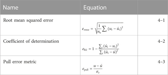
TABLE 1. Error metrics used in this work.
In contrast to the first two, the pull metric
2.2 Data flow for machine learning
The development of the data-driven models follows the data flow introduced by (Brockkötter et al., 2020; Brockkötter et al., 2021). The data flow consists of five steps, including (i) data transformation, (ii) data split, (iii) machine learning (ML), (iv) selection of the data-driven algorithm, and (v) wrapper feature selection. In the first two steps, the database is transformed by applying a Min Max scaler and split randomly into a train and a test part with a ratio of 85/15. The split is performed once before training and not altered thereafter to ensure comparability of the following development steps. The transformed and split data set is used to train six potential machine learning algorithms, including (i) linear regression, (ii) k-Nearest Neighbor, (iii) support-vector-regression, (iv) Gaussian processes, (v) decision tree, and (vi) random forest. In contrast to (Brockkötter et al., 2020), we did not consider Artificial Neural Networks (ANN) as the mismatch between the size of our data sets and the model complexity of ANNs would not justify the use of such a complex algorithm. The training of all ML algorithms is divided into two consecutive steps. First, the training of all ML algorithms is performed based on an exhaustive grid search with k-fold cross-validation with
2.3 Revised breakage model
The white-box part of the hybrid breakage model is based on a revised form of Garthe’s breakage model. Garthe’s model was chosen for this purpose as, in principle, it is not bound to a specific breakage mechanism, but rather replicates the form of the breakage probability between the boundary values
For
The first term on the right side of Eq. 2–1 limits the
2.4 Breakage database
The breakage database for PSEs consists of 743 data sets retrieved from literature (Haverland, 1988; Eid et al., 1991; Wagner, 1994; Garthe, 2006). One data set corresponds to one entry in the breakage database which specifies the experimental value of the breakage probability
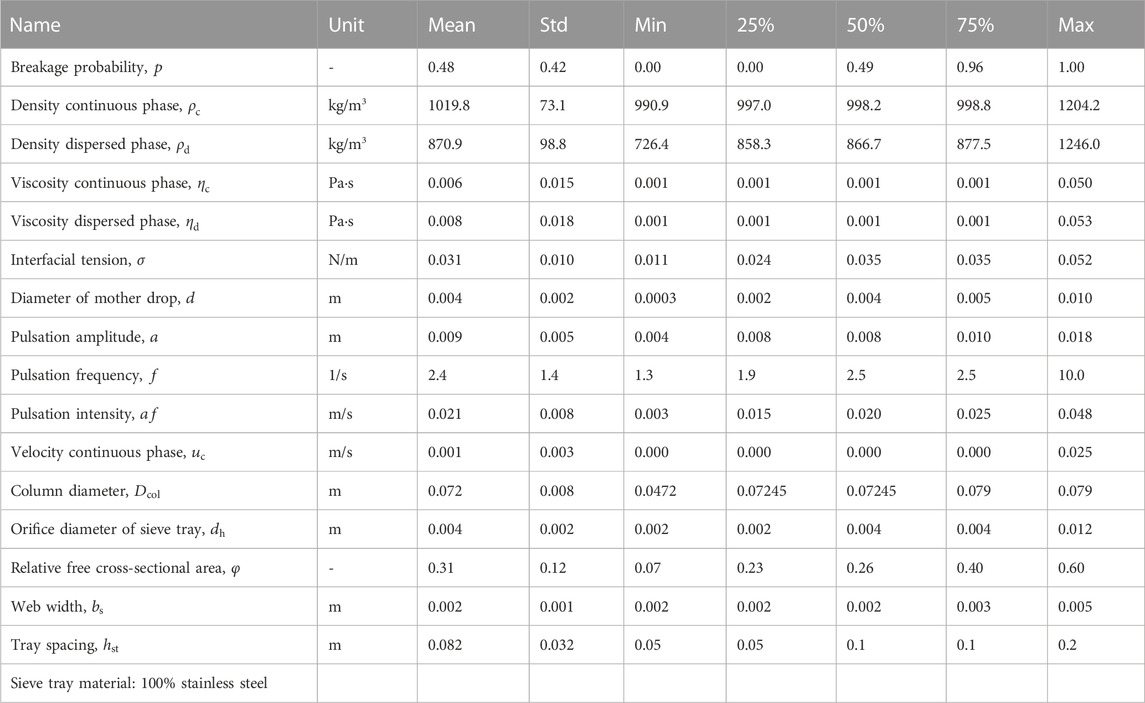
TABLE 2. Statistical information on the breakage database.
The experimental values for
3 Results and discussion
3.1 Hybrid breakage model
The revised breakage model introduced in section 2.3 poses the prerequisite for a robust breakage model, due to a physically consistent prediction of drop breakage between
In the following, we address these limitations by introducing PEM for
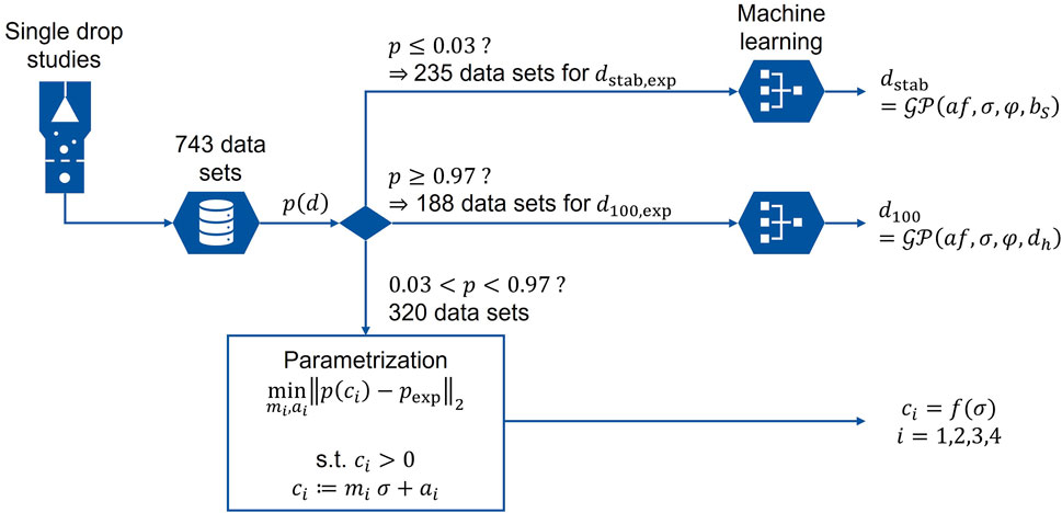
FIGURE 4. Dataflow for the development of the hybrid breakage model.
In the following, the results of the PEM development for
3.1.1 Modeling of
The data sets for
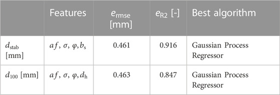
TABLE 3. Final data-driven models for
The feature set included in the final models agrees well with most physical-empirical correlations for
3.1.2 Continuous parameter estimation for
For the development of PEMs for the breakage model parameters
w.r.
The results of the parameterization are summarized in Table 4. The table shows the eight parameters

TABLE 4. Results of constant and linear parametrization of the hybrid breakage model and residues of the hybrid breakage model and Garthe’s model. The original parameterization of Garthe’s model depends on multiple influencing factors. Thus, the entries are marked with the non-zero marker ∗. The numerical values for ∗ are listed in the Supplementary Material.
3.1.3 Model validation
In the final step of the model development, the revised breakage model is extended by the data-driven PEM for
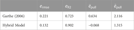
TABLE 5. Error metrics of Garthe’s and the hybrid breakage model for the prediction of the breakage probability on the complete breakage database.
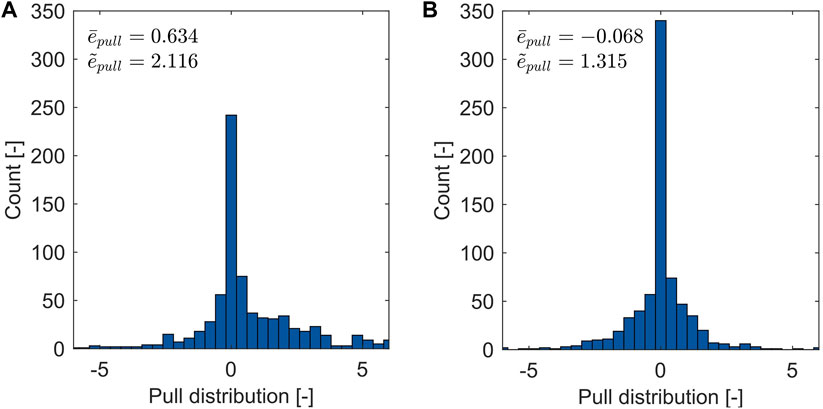
FIGURE 5. Pull distribution of Garthe’s (A) and the hybrid breakage model (B) for the prediction of the breakage probability on the complete breakage database.
Regarding the pull distribution, both models are centered around 0 and have a qualitatively reasonable spread around the center point. The hybrid model predicts a larger fraction of the database within the assumed measurement accuracy, while the variance is obviously smaller. The qualitative observation is numerically confirmed: the hybrid model achieves a prediction accuracy close to the optimal value of 0, underestimating it slightly (
Finally, a qualitative evaluation based on Figure 5 indicates that both models can correctly depict the experimental breakage probability in the database. Nevertheless, the hybrid model achieves better scores in all error metrics and has an extended validity range due to the PEMs for
3.2 Sensitivity analysis
The purpose of the sensitivity analysis is to test the model’s ability to predict physically consistent trends of
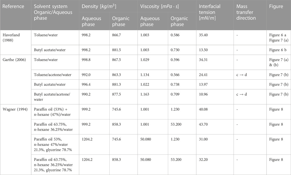
TABLE 6. Properties of the solvents considered in the sensitivity analysis.
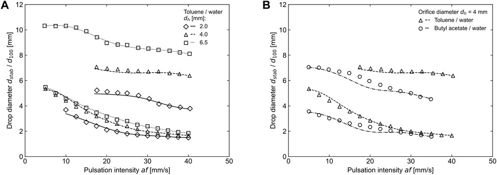
FIGURE 6. (A) Comparison of
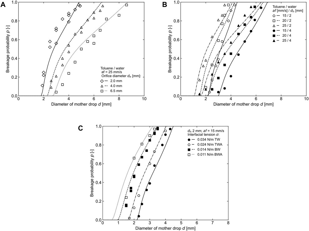
FIGURE 7. Breakage probability for toluene/water for (A) different orifice diameters, (B) different orifice diameters and pulsation intensities, and (C) for different interfacial tensions. Experimental data: symbols, prediction: lines. Figures according to (Haverland, 1988; Garthe, 2006).
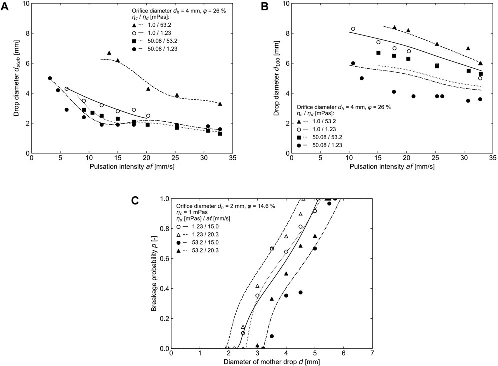
FIGURE 8. Comparison of (A)
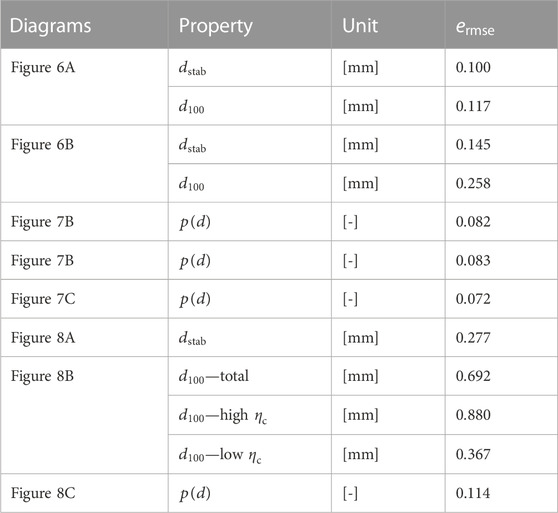
Three overall
- Trend 1: Higher
- Trend 2: Lower
- Trend 3: Higher
Trends 1 and 2 can be accounted for by a force balance of stabilizing and disruptive forces acting on the drop surface and deforming the shape of the drop. In principle, the force balance is incorporated in the
Considering the prediction of
In contrast, Wagner’s data sets include rather unconventional solvent systems, which can be distinguished primarily based on the viscosities
Apart from the trends already discussed for the EFCE systems, one additional trend can be deduced from Wagner’s experiments.
- Trend 4: Higher
Wagner argues that a highly viscous continuous phase increases the shear stress on the drops during orifice passage, increasing the tendency to drop breakage (see
Although both viscosities
The validity of the
Overall, the prediction of the hybrid breakage model is consistent with the trends in the experimental data for
4 Conclusion
Within this study, we have developed a hybrid breakage model for PSEs based on a serial hybrid modeling approach. The hybrid breakage model consists of an empirical model basis which is enhanced by data-driven PEMs. For the model basis, Garthe’s breakage model was revised to guarantee a physically consistent prediction of the breakage probability
For validation purposes, the complete breakage database was predicted by Garthe’s and the hybrid breakage model, respectively. Subsequently, the accuracy of both models was compared based on the pull distribution of their predictions. Thereby, the hybrid model not only surpassed Garthe’s model regarding the prediction error (hybrid:
Regarding the research on drop breakage, we would suggest two aspects to be considered for future studies. As demonstrated in Section 3.2, a limited variety in the training data of the data-driven PEM can substantially affect the quality of the model. Consequently, future studies should focus on solvent systems beyond the EFCE solvents. Special effort should be put in the investigation of highly viscous solvents as was done for agitated systems in recent years. The second aspect we would suggest concerns the model development itself. In this study, we focused primarily on the reduction of the number of features considered for the PEM development. The reduction of the feature space addresses the problem that every additional feature in a data-driven model improves the error metrics, yet simultaneously reduces the validity range, e.g., convex hull. In future studies, a reduction of the number of parameters should be considered as a possible objective too. For example, the breakage probability might be expressed by a simpler breakage model eventually with fewer parameters than
Data availability statement
The original contributions presented in the study are included in the article/Supplementary Material, further inquiries can be directed to the corresponding author.
Author contributions
AP: Conceptualization, Data curation, Formal Analysis, Investigation, Methodology, Project administration, Software, Supervision, Validation, Visualization, Writing–original draft, Writing–review and editing. JR: Conceptualization, Data curation, Formal Analysis, Investigation, Methodology, Software, Visualization, Writing–review and editing, Writing–original draft, Validation. HG: Data curation, Methodology, Writing–review and editing, Software. AJ: Supervision, Writing–review and editing.
Funding
The author(s) declare that no financial support was received for the research, authorship, and/or publication of this article.
Conflict of interest
The authors declare that the research was conducted in the absence of any commercial or financial relationships that could be construed as a potential conflict of interest.
Publisher’s note
All claims expressed in this article are solely those of the authors and do not necessarily represent those of their affiliated organizations, or those of the publisher, the editors and the reviewers. Any product that may be evaluated in this article, or claim that may be made by its manufacturer, is not guaranteed or endorsed by the publisher.
Supplementary material
The Supplementary Material for this article can be found online at: https://www.frontiersin.org/articles/10.3389/fceng.2023.1274349/full#supplementary-material
Abbreviations
ANN, Artificial neural network; BW, Butyl acetate/water; BWA, Butyl acetate/water/acetone; EFCE, European Federation of Chemical Engineering; GP, Gaussian Process; ML, Machine learning; PBM, Population balance model; PEM, Parameter estimation model; PSE, Pulsed sieve-tray extraction column; Sec, Section; TW, Toluene/water; TWA, Toluene/water/acetone.
References
Brockkötter, J., Ahndorf, J., and Jupke, A. (2021). Prediction of flooding in packed liquid-liquid and high-pressure extraction columns using a Gaussian process. Chem. Ing. Tech. 93, 1907–1916. doi:10.1002/cite.202100073
Brockkötter, J., Cielanga, M., Weber, B., and Jupke, A. (2020). Prediction and characterization of flooding in pulsed Sieve Plate Extraction columns using data-driven models. Ind. Eng. Chem. Res. 59, 19726–19735. doi:10.1021/acs.iecr.0c03282
Cramer, E., and Kamps, U. (2017). Grundlagen der Wahrscheinlichkeitsrechnung und Statistik: Eine Einführung für Studierende der Informatik, der Ingenieur-und Wirtschaftswissenschaften. Berlin: Springer Spektrum.
Dahmen, W., and Reusken, A. (2022). Numerik für Ingenieure und Naturwissenschaftler. Berlin [u.a.]: Springer.
Eid, K., Gourdon, C., Casamatta, G., and Muratet, G. (1991). Drop breakage in a pulsed sieve-plate column. Chem. Eng. Sci. 46, 1595–1608. doi:10.1016/0009-2509(91)87008-Z
Gameiro, M. L. F., Machado, R. M., Ismael, M. R. C., Reis, M. T. A., and Carvalho, J. M. R. (2010). Copper extraction from ammoniacal medium in a pulsed sieve-plate column with LIX 84-I. J. Hazard. Mater. 183, 165–175. doi:10.1016/j.jhazmat.2010.07.006
Garthe, D. (2006). [München]: Technical University of Munich. Fluiddynamics and Mass Transfer of Single Particles and Swarms of Particles in Extraction Columns. [Dissertation].
Gourdon, C., Casamatta, G., and Angelino, H. (1991). Single drop experiments with liquid test systems: a way of comparing two types of mechanically agitated extraction columns. Chem. Eng. J. 46, 137–148. doi:10.1016/0300-9467(91)87005-U
Hasan, B. O. (2017). Breakage of drops and bubbles in a stirred tank: a review of experimental studies. Chin. J. Chem. Eng. 25, 698–711. doi:10.1016/j.cjche.2017.03.008
Haverland, H. (1988). Untersuchungen zur Tropfendispergierung in flüssiigkeitspulsierten Siebboden-Extraktionskolonnen. [Dissertation]. Clausthal: Technical University of Clausthal.
Haverland, H., Vogelpohl, A., Gourdon, C., and Casamatta, G. (1987). Simulation of fluid dynamics in a pulsed sieve plate column. Chem. Eng. Technol. 10, 151–157. doi:10.1002/ceat.270100119
Henschke, M. (2003). Auslegung pulsierter siebboden-extraktionskolonnen. [Habilitation]. [Aachen]: RWTH Aachen University.
Hlawitschka, M. W., Schulz, J., Wirz, D., Schäfer, J., Keller, A., and Bart, H.-J. (2020). Digital Extraction Column: measurement and modeling techniques. Chem. Ing. Tech. 92, 914–925. doi:10.1002/cite.202000043
James, G., and Witten, D. (2013). #x88;An introduction to statistical learning: with applications in R. New York: Springer. [etc.].
Jaradat, M., Attarakih, M., and Bart, H.-J. (2011a). Advanced prediction of pulsed (packed and sieve plate) extraction columns performance using population balance modelling. Chem. Eng. Res. Des. 89, 2752–2760. doi:10.1016/j.cherd.2011.05.009
Jaradat, M., Attarakih, M., and Bart, H.-J. (2011b). Population balance modeling of pulsed (packed and sieve-plate) extraction columns: coupled hydrodynamic and mass transfer. Ind. Eng. Chem. Res. 50, 14121–14135. doi:10.1021/ie201041q
Jareš, J., and Procházka, J. (1987). Break-up of droplets in Karr reciprocating plate extraction column. Chem. Eng. Sci. 42, 283–292. doi:10.1016/0009-2509(87)85058-3
Kahrs, O., and Marquardt, W. (2007). The validity domain of hybrid models and its application in process optimization. Chem. Eng. Process. Process Intensif. 46, 1054–1066. doi:10.1016/j.cep.2007.02.031
Kalem, M. (2015). Einzeltropfenbasierte Simulation von pulsierten Siebbodenextraktionskolonnen für die Reaktivextraktion. [Dissertation]. Aachen: RWTH Aachen University.
Kolmogorov, A. N. (1991). The local structure of turbulence in incompressible viscous fluid for very large Reynolds numbers. Proc. R. Soc. Lond. A 434, 9–13. doi:10.1098/rspa.1991.0075
Kraume, M., Gäbler, A., and Schulze, K. (2004). Influence of physical properties on drop size distribution of stirred liquid-liquid dispersions. Chem. Eng. Technol. 27, 330–334. doi:10.1002/ceat.200402006
Kumar, A., and Hartland, S. (1995). A unified correlation for the prediction of dispersed-phase hold-up in liquid-liquid extraction columns. Ind. Eng. Chem. Res. 34, 3925–3940. doi:10.1021/ie00038a032
Lagarias, J. C., Reeds, J. A., Wright, M. H., and Wright, P. E. (1998). Convergence properties of the nelder-mead simplex method in low dimensions. SIAM J. Optim. 9, 112–147. doi:10.1137/S1052623496303470
Maaß, S., Rojahn, J., Hänsch, R., and Kraume, M. (2012). Automated drop detection using image analysis for online particle size monitoring in multiphase systems. Comput. Chem. Eng. 45, 27–37. doi:10.1016/j.compchemeng.2012.05.014
McBride, K., Sanchez Medina, E. I., and Sundmacher, K. (2020). Hybrid semi-parametric modeling in separation processes: a review. Chem. Ing. Tech. 92, 842–855. doi:10.1002/cite.202000025
R. Goedecke (Editor) (2006). Fluidverfahrenstechnik: geschichte, methodik, praxis, technik (Weinheim, Chichester: Wiley-VCH Verlag GmbH; John Wiley & Sons).
Schügerl, K. (1994). Solvent extraction in biotechnology: recovery of primary and secondary metabolites. Springer-Verlag.
Stamatoudis, M., and Tavlarides, L. L. (1985). Effect of continuous-phase viscosity on the drop sizes of liquid-liquid dispersions in agitated vessels. Ind. Eng. Chem. Proc. Des. Dev. 24, 1175–1181. doi:10.1021/i200031a047
Thompson, M. L., and Kramer, M. A. (1994). Modeling chemical processes using prior knowledge and neural networks. AIChE J. 40, 1328–1340. doi:10.1002/aic.690400806
T. C. Lo, M. H. I. Baird, and C. Hanson (Editors) (1983). Handbook of solvent extraction (New York: Wiley).
T. Mísek (Editor) (1985). Standard test systems for liquid extraction (Rugby: Institution of Chemical Engineers).
Wagner, G. (1994). Der Einfluss der Viskosität auf die Strömung in Apparaten für die Flüssig-flüssig-Extraktion. [Dissertation]. [Munich]: Technical University of Munich.
Weber, B., and Jupke, A. (2020). Compartment-model for the simulation of the separation performance of stirred liquid–liquid-extraction columns. AIChE J. 66. doi:10.1002/aic.16286
Weber, B., Meyer, C., and Jupke, A. (2019). Performance map for the design of liquid-liquid extraction columns. Chem. Ing. Tech. 91, 1674–1680. doi:10.1002/cite.201900057
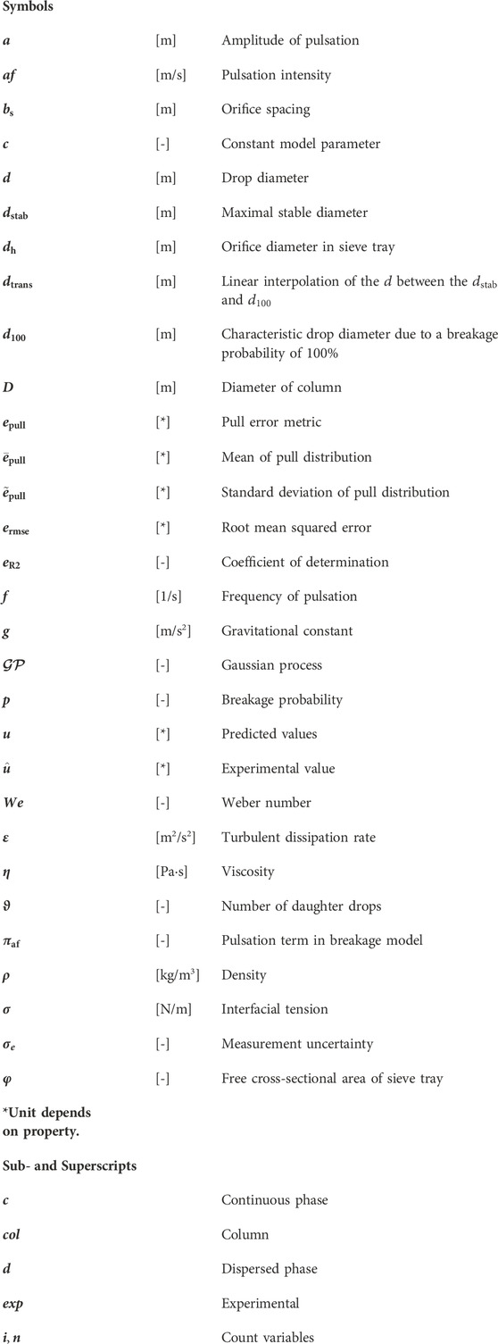
Nomenclature
Keywords: pulsed sieve tray extraction column, liquid-liquid extraction, drop breakage, hybrid model, population balance model
Citation: Palmtag A, Rousselli J, Gröschl H and Jupke A (2023) Hybrid modeling of drop breakage in pulsed sieve tray extraction columns. Front. Chem. Eng. 5:1274349. doi: 10.3389/fceng.2023.1274349
Received: 08 August 2023; Accepted: 05 October 2023;
Published: 08 November 2023.
Edited by:
Hans-Jörg Bart, University of Kaiserslautern, GermanyReviewed by:
Matthaeus Siebenhofer, Graz University of Technology, AustriaVille Alopaeus, Aalto University, Finland
Copyright © 2023 Palmtag, Rousselli, Gröschl and Jupke. This is an open-access article distributed under the terms of the Creative Commons Attribution License (CC BY). The use, distribution or reproduction in other forums is permitted, provided the original author(s) and the copyright owner(s) are credited and that the original publication in this journal is cited, in accordance with accepted academic practice. No use, distribution or reproduction is permitted which does not comply with these terms.
*Correspondence: Andreas Jupke, YW5kcmVhcy5qdXBrZUBhdnQucnd0aC1hYWNoZW4uZGU=