The evolution of heat exposure in changing societies and a changing climate from 1960 to 2100

With climate change, human exposure to heat has increased over recent decades and is expected to substantially increase in the future. This study introduces a novel metric – namely, the exponentially weighted degree-day approach – to assess population-weighted heat exposure at the national level, incorporating both static and dynamic population scenarios. Using ERA5 reanalysis and CMIP6 climate projections under the SSP2-4.5 and SSP5-8.5 scenarios, we analyze and categorize global heat exposure and its trends from 1960 until 2100. Our findings reveal a significant rise in heat exposure over past decades, disentangling the contributions of climate and demographic changes. Furthermore, a thorough analysis of biases across different datasets and model dimensions provides a global perspective based on daily maximum and daily mean temperatures. This analysis forms the basis for quantifying current and future heat exposure, together with a qualitative heat zone classification scheme. The results underscore the urgent need for targeted adaptation strategies and improved climate metrics to better assess and mitigate future heat-related risks.

1 Introduction

Global temperatures have been rising for several decades and will continue to do so, depending on the pathway of anthropogenic climate change. With rising temperatures, heat waves are becoming more frequent in more regions around the world. They are a social burden, and their link to climate change is of great relevance due to the increasing temperature near the surface and increasing humidity, according to the so-called Clausius-Clapeyron scaling (Marx et al., 2021). Extreme summer temperatures have repeatedly caused significant excess mortality (Gasparrini et al., 2015), especially among vulnerable populations, as seen in the years 2003 (Kosatsky, 2005), 2015 (Muthers et al., 2017), 2019 (Klimiuk et al., 2024), 2022 (Ballester et al., 2023), and also 2023 (Gallo et al., 2024) in Central Europe. Beyond mortality, increased temperatures and humidity have a direct impact on health and labor productivity (Szewczyk et al., 2021; Kjellstrom et al., 2018), and wellbeing (Zhao et al., 2021). They also result in a change in climate zones, with consequences, for example, for infectious diseases (Semenza and Menne, 2009) or an increase in heat stress and cooling costs (Hooyberghs et al., 2017; Hundhausen et al., 2023; Saeed et al., 2021).

Beyond regional climate trends, urban areas are significantly more affected by increased temperatures than rural areas (Holmer and Eliasson, 1999). More than 50% of the world's population lives in urban areas (Zhou et al., 2018), although these regions only cover 3% of Earth's total land surface (Eugenio Pappalardo et al., 2023). The concentrated development of living space within these urban landscapes results in dense built structures with reduced vegetation and increased surface sealing. This leads to a modified thermal climate in which temperatures are elevated compared to the rural countryside. This phenomenon is called the urban heat island (UHI) effect and is especially pronounced during the night (Voogt and Oke, 2003). Due to the relatively small spatial extent and highly heterogeneous nature of cities, UHI effects are insufficiently represented in global climate models. The coarse grid resolution of ERA5 reanalysis, as well as the lack of urban process parameters, contribute to the neglect of UHI effects in this dataset (Nogueira et al., 2022; Adinolfi et al., 2023). Consequently, small-scale temperature extremes are poorly captured by coarse global models, potentially leading to an under representation of the heat exposure experienced by urban residents. Nonetheless, both downscaled climate models as well as ERA5 are the global standard for climate analysis and are, despite their limitations, useful for any kind of global analysis.

In our study, we focus on the concept of heat exposure by assessing the annual amount of daily mean and maximum temperatures affecting the population in a certain country. However, the change in heat stress on human exposure is determined not only by climate alone. Demographic changes, including population growth, urbanization, and migration, also shape how and where people are exposed to heat and heat extremes (Jones et al., 2015; Rohat et al., 2019). Yet, most of the existing literature focuses mainly on climatic variables without explicitly accounting for changes in the population distribution over time (Matthews et al., 2017; Schwingshackl et al., 2021a). Thus, the relative impacts of changes in population distribution and temperature trends has not yet been sufficiently disentangled yet.

To address this gap, we assess changes in heat exposure driven by both climatic and demographic trends. Specifically, we focus on annual changes in degree-days based on daily mean and maximum temperatures per country. In doing so, we consider both a static and dynamic spatial population distributions. This is carried out for the historic period of 1960–2024 and for different climate pathways, including the historical baseline of CMIP6 from 1960 to 2014 and the climate scenarios of SSP2-4.5 and SSP5-8.5 for 2015–2100.

In summary, we provide three different perspectives. First, we assess the impact of population dynamics on heat exposure since 1960. Second, we compare ERA5 and CMIP6 results for both the historical reference period and the initial decade of the climate projection from 2015 to 2024. Finally, we assess the development of heat exposure for future decades up to 2100 and provide a qualitative classification scheme for heat exposure to better compare and communicate the results. This way, we want to resolve how historical changes in climate and population have contributed to heat exposure, how it might continue in the upcoming decades, and how temperatures from climate models correlate to historical observations. All steps are conducted on a national basis to provide valuable insights for policymakers to anticipate future challenges related to social and infrastructural heat impacts.

2 Data

2.1 Climate data

Historical temperature data were obtained from the ERA5 reanalysis dataset of the European Centre for Medium-Range Weather Forecasts (ECMWF; Hersbach et al., 2020). This dataset, which is widely used for global and regional historical climate assessments, provides a global coverage of hourly data on a 0.25° × 0.25° spatial resolution since 1940. Covering the period from 1960 to 2024, the hourly surface air temperature at 2 m above the ground was aggregated to retrieve daily maximum temperatures (tasmax) and daily mean temperatures (tas).

Future projections of daily maximum temperatures were derived from the Global Downscaled Projections for Climate Impacts Research (GDP-CIR) CMIP6 dataset (Thrasher et al., 2022), which is publicly available. This dataset provides bias-corrected and downscaled climate model data based on the Scenario Model Intercomparison Project (ScenarioMIP; O'Neill et al., 2016) of CMIP6 (CMIP6; Eyring et al., 2016) for daily minimum and maximum temperatures. The bias correction and downscaling of this dataset were done using quantile data mapping (Cannon et al., 2015) and quantile-preserving localized-analog downscaling based on ERA5. This ensures that the full range of climate variability from the original data is realistically represented in the downscaled data. The raw output from global climate models within CMIP6 would be too coarse in resolution; thus, the downscaling component of this dataset, with a resolution of about 25 km, makes it directly compatible with ERA5. However, this dataset does not explicitly provide daily mean temperatures. Thus, they are considered as the mean between the daily maximum and minimum values.

It should be noted that such global climate models come with various limitations, including insufficient capturing of extreme values (e.g., strong wind or precipitation) as well as limitations in identifying very regional climate patterns (e.g., severe convective storms or topographic effects). Even bias corrected models usually do not suffice to overcome these limits (Ehret et al., 2012; Casanueva et al., 2020). For this study, we utilized 15 individual climate models as well as the ensemble for 2 shared socio-economic pathways (SSP) (SSPs; Riahi et al., 2017). SSP2-4.5 describes a stabilizing pathway with intermediate emissions and climate protection measures in place. In contrast, SSP5-8.5 describes the high-emission scenario representing fossil-fueled development. While SSP2-4.5 can be anticipated as a potential outcome of global policies, the “Middle of the Road” which still ends well above the 2 °C Paris climate goal with a global warming of 2.1–3.5 °C, SSP5-8.5 can be considered the worst-case climate scenario under a failure of global climate protection efforts and an extensive fossil fuel industry with average global temperatures increasing by 3.3–5.7 °C (Riahi et al., 2017).

In total, 15 individual models and their ensemble mean have been taken into account (see Table 1). Similar to ERA5, this data is also provided at a spatial resolution of 0.25° × 0.25°. For comparison, the historic baseline from 1960–2014 is considered, as well as the respective climate projections from 2015–2100, covering a whole century of climate change.

Table 1

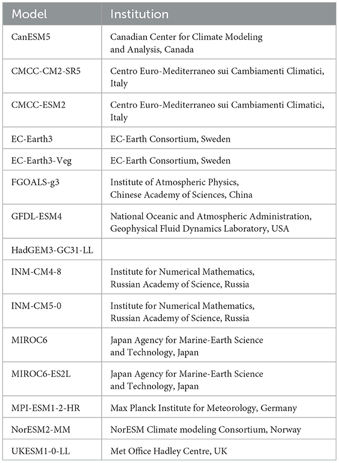
Table 1. List of used bias-corrected and downscaled CMIP6 models (historical, SSP245 and SSP585 runs) from Thrasher et al. (2022).

2.2 Population data

As a starting point for the spatial aggregation of heat exposure, the 2023 version of the Global Human Settlement Layer (GHSL) population model was used. This model is supported by the European Commission, Joint Research Centre, and Directorate-General for Regional and Urban Policy (Schiavina et al., 2023; Freire et al., 2016). The GHSL is the source of new global spatial information, evidence-based analysis, and knowledge about human presence on the planet. It provides spatial rasters with different resolutions on the population distribution in 5 year increments between 1975 and 2030. Here, we used data on a 1 km raster as starting point. To assess years prior to 1975, we applied the 1975 population distribution as a static approximation to account for the lack of reliable spatial data for earlier years. For all other years, population distributions were linearly interpolated between GHSL's reference years to acquire annual population distribution maps from 1960 to 2024. For future projections, we use a static population scenario, considering 2020 as the reference year.

3 Methodology

3.1 Preprocessing

To get the data ready for computing heat exposure, some preprocessing was necessary. First, the geographic scope was constrained to territorial states. With the initial climate rasters on an approximately 25 km sized grid cells, very small countries and especially small island states are not appropriately represented. Thus, those small nations have been excluded from the assessment. This results in approximately 190 countries worldwide being available for the computation of heat exposure statistics.

Next, it was necessary to bring both population and climate rasters to the same spatial resolution. This was done by linear 2D spline interpolation onto a global 10 km grid for both population and climate, increasing the resolution of climate rasters and decreasing it for the population rasters. The increase of spatial resolution in the climate data does not improve the spatial details of the raw climate data, but allows for a more efficient data processing down the line. Since only the relative population distribution is relevant in this approach, as outlined below, ensuring that the absolute population distribution remained intact across every year when resampling its spatial resolution was not necessary. Finding a middle ground on spatial resolution was the most feasible approach with respect to computational efficiency while staying as close to the original data resolution as possible. Individual grid cells were then exclusively assigned to their closest country.

3.2 Heat exposure

To assess the impact of increasing heat on people, a spatial correlation of population statistics and temperature data was conducted. This approach integrates climate and population data on a daily basis, which allows for both a static and dynamic perspective on population distribution. It builds upon the concept of degree-days, which has been widely used in the field of agriculture and energy consumption to measure heat accumulation over a certain time period (Mourshed, 2012; Bai et al., 2025). However, in this application, temperatures are not summed linearly, but exponentially to better capture the nonlinear human vulnerability to extreme heat (e.g., Huang et al., 2022; Lo et al., 2023; Sherwood and Huber, 2010; Mora et al., 2017).

This methodology follows three key steps. First, we compute daily population-weighted temperature histograms for each country and year. Second, these histograms are normalized and weighted exponentially by temperature. Finally, annual aggregation and logarithmic transformation provide a country-level annual heat exposure index, which we call the representative temperature T_rep. These steps are explained in further detail in the next paragraphs.

For each country c, year y, and day d, we computed a histogram describing how many people have been exposed to a specific daily temperature. This was done for every grid cell i within a country. P(i, y) then describes the population in year y and cell i with its respective daily average or maximum temperature T(i, d, y). Then, the histogram value for a specific temperature bin T can be calculated as:

$\begin{array}{ll}H(c,d,y,T)={\displaystyle \sum _{i\in c}}\delta (T(i,d,y)-T)\times P(i,y)& (1)\end{array}$

where δ denotes the binning function to group the population into discrete temperature bins depending on T. This was done across all climate models, their respective time frames, and countries.

These histograms were then normalized by dividing them by the total population within a country and weighted by the temperature weighting term W(T). This term was defined for temperatures above 10 °C and 0 otherwise. This exponential form was chosen to strongly emphasize the impact of higher temperatures, consistent with known nonlinear physiological responses, while the 10 °C threshold focused the analysis on warmer conditions relevant to heat stress. Alternative formulations exist, but this form provides the necessary sensitivity for our comparative analysis. This led to the normalized daily heat exposure $\tilde{H}(c,d,y)$.

$\begin{array}{ll}\tilde{H}(c,d,y,T)=W(T)\times \frac{H(c,d,y,T)}{{\displaystyle {\sum }_{i\in c}}P(i,y)}& (2)\end{array}$

$\begin{array}{ll}W(T)=\{\begin{array}{ll}\exp (T-10),\hfill & \text{if }T\ge {10}^{\circ }\text{C}\hfill \\ 0,\hfill & \text{if }T<{10}^{\circ }\text{C}\hfill \end{array}& (3)\end{array}$

Here, population is used to spatially weight the climate variable. Thus, the absolute population is of lesser importance than its relative spatial distribution. This reduces uncertainties arising due to resampling of the input data to a desired resolution and from their absolute values.

Finally, the normalized heat exposure is summed and log-normally transformed to retrieve the annual heat exposure, which we can also call the representative temperature T_rep(c, y) for country c and year y. The annual sum of daily weighted exposures:

$\begin{array}{ll}{T}_{rep}(c,y)=ln({\displaystyle \sum _{d=1}^D}{\displaystyle \sum _T}\tilde{H}(c,d,y,T))& (4)\end{array}$

This approach reduces the total heat exposure of a country to a single value. T_rep can be computed based on different daily temperature statistics. In the following, we will use $T_{rep}^{tasmax}$ for statistics based on daily maximum temperatures and $T_{rep}^{tas}$ for statistics using daily mean temperatures. Values of $T_{rep}^{tasmax}$ typically range from 20°C to 40°C and from 10°C to 30°C for $T_{rep}^{tas}$. While providing a single value per country-year, T_rep is treated as a dimensionless index primarily intended for comparing relative exposure changes across regions and scenarios, rather than as an absolute physical temperature.

3.3 Population scenarios

To disaggregate the influence of population and climate on heat exposure, we considered 2 different population scenarios. First, we computed the annual heat exposure assuming a static population distribution. For this, we applied the 2020 population distribution model to all years, assuming a changing climate as if it would affect the 2020 population. Second, we applied the changing population distribution as modeled by Schiavina et al. (2023) for the years 1975 to 2025 in 5-year increments. As outlined above, for years within the increments, the population distribution was linearly interpolated.

Both static and dynamic population scenarios were then applied to recompute heat exposure based on the ERA5 historical reanalysis data from 1960 to 2024. Heat exposure computed based on CMIP6 models considered only a static population distribution, since the spatial population distribution models already end in 2030, making them irrelevant for use for the upcoming decades. Thus, CMIP6 future projections were computed with a constant 2020 population model to remain consistent with the static population scenario.

To identify potential biases within and between different model components, we introduced several assessment metrics.

To quantify the relevance of changes in the population distribution, we compared heat exposure for two different periods and under two different population scenarios. The first scenario assumes a dynamic population development as given by the data from GHSL, while the second assumes a constant population distribution based on the year 2020.

This allows us to compute the change in heat exposure based on population changes $\Delta T_{rep}^{pop}$ between two points in time, which can be computed as:

$\begin{array}{l}\Delta T_{rep}^{pop}=(T_{rep}^d(c,t_2)-T_{rep}^d(c,t_1))-(T_{rep}^s(c,t_2)\\ -T_{rep}^s(c,t_1))t_2>t_1& (5)\end{array}$

Here, $T_{rep}^d(c,t_x)$ describes the representative temperature at time t_x considering a dynamic population scenario and $T_{rep}^s(c,t_x)$ the same for a static population model. Here, t₂ is a later point in time than t₁. To get robust results, it is recommended that t₁ and t₂ are not single-year statistics, but the average across a timespan of e.g., +/–15 around t₁ and t₂ respectively. When referencing certain years in time in the following sections, the respective 30-year average is meant.

Heat exposure can be influenced by epistemic and aleatoric uncertainties. To address those when quantifying biases for future decades, we introduce an indicator system based on 3 different model domains. The first indicator captures whether heat exposure has been previously influenced by population dynamics; the second captures the long-term historical bias when comparing ERA5 and CMIP6 historical reference period; the last one compares the first decade of climate projections of 2015–2024. Due to the high uncertainties in modeling, we reduce the potential values of each indicator to –1, 0, and +1 to acquire a robust indicator metric.

The index I_p identifies whether population dynamics have significantly influenced heat exposure from 1975 to 2020. If population dynamics contributed more than the threshold t_p, I_p becomes +1, if they reduced it by at least t_p then I_P = −1:

$\begin{array}{ll}{I}_p=\{\begin{array}{ll}+1,\hfill & \text{if }\Delta T_{rep}^{pop}/\Delta T_{rep}>+t_p\%\hfill \\ -1,\hfill & \text{if }\Delta T_{rep}^{pop}/\Delta T_{rep}<-t_p\%\hfill \\ 0,\hfill & \text{else}\hfill \end{array}& (6)\end{array}$

Here, ΔT_rep describing the heat exposure change assuming the static population of 2020 and $\Delta T_{rep}^{pop}$ represents the change resulting only from dynamics in temperature and population from the years 1975 to 2020. We apply the same logic for I_h and I_r. I_h is the indicator based on the error between CMIP6 and ERA5 for the historical reference period of 1960 to 2014. Similarly, I_r is the indicator based on the error between CMIP6 and ERA5 for the latest decade of 2015 to 2024 as described above. In both cases, if the error is larger than t_h|t_r, I_r, or I_h are +1; if the error is smaller than t_h|t_r, then I_r or I_h are –1.

$\begin{array}{ll}{I}_h=\{\begin{array}{ll}-1,\hfill & \text{if }\Delta {\overline{T}}_{rep}(\tau )<-t_h\hfill \\ +1,\hfill & \text{if }\Delta {\overline{T}}_{rep}(\tau )>+t_h\hfill \\ 0,\hfill & \text{else}\hfill \end{array}\text{\hspace{1em}with\hspace{1em}}\tau =[1960,2015]& (7)\end{array}$

$\begin{array}{ll}{I}_r=\{\begin{array}{ll}-1,\hfill & \text{if }\Delta {\overline{T}}_{rep}(\tau )<-t_r\hfill \\ +1,\hfill & \text{if }\Delta {\overline{T}}_{rep}(\tau )>+t_r\hfill \\ 0,\hfill & \text{else}\hfill \end{array}\text{\hspace{1em}with\hspace{1em}}\tau =[2015,2024]& (8)\end{array}$

Here, $\Delta {\overline{T}}_{rep}(\tau )$ describes the average difference between T_rep from CMIP6 and ERA5 for a period τ; for the historical indicator I_h, this period is 1960 to 2014. I_r is defined the same way, but with τ = [2015, 2024]. For this period, CMIP6 data have been averaged across SSP2-4.5 and SSP5-8.5 to avoid uncertainties from the respective input models. This is a valid approach since relevant differences in climate forcing due to the different emission scenarios do not occur before 2030.

We apply this to results from both tas and tasmax leading to 6 separate indicators. Thus, the total indicator of over- or underestimation, I_t, ranges from –6 to +6.

$\begin{array}{ll}I={\displaystyle \sum _{i\in \left[p,h,r\right]}^{tas}}{I}_i+{\displaystyle \sum _{i\in \left[p,h,r\right]}^{tasmax}}{I}_i& (9)\end{array}$

This indicative approach provides a qualitative way to showcase potential model biases and avoids the introduction of potentially highly uncertain quantitative adjustments. It combined the assessment of models errors both on the climatological scale at 2 time frames as well as errors potentially introduced by changes in the population pattern. Thus, we can directly use CMIP6 model results and qualitatively highlight whether they under- or overestimate heat exposure based on the given indication.

4 Results

The results can be broken down into three major parts. The first part considers how heat exposure is influenced by population dynamics. Second, we compare the historical period of CMIP6 with observations from ERA5 to identify biases of over- and underestimation of heat exposure. Finally, we assess heat exposure biases for future decades under CMIP6 SSP2-4.5 and SSP5-8.5 by applying our previous findings.

4.1 Population dynamics

To assess the contribution of population dynamics to changes in heat exposure, we compare the change in heat exposure between the 1980s (1980–1989) and the 2020s (2015–2024) under two different population scenarios. Here, we consider the difference in heat exposure changes between the static and dynamic population distributions, denoted as $\Delta T_{rep}^{pop}$. If the heat exposure change is larger for the dynamic population scenario, then the changes in the spatial population distribution account for increased heat exposure. On the other hand, if the static population scenario leads to a larger change in heat exposure, then the changes in population distribution have counteracted the climate change signal.

In general, population distribution plays a critical role in heat exposure, especially for large countries with a diverse bioclimatic landscape covering different climate zones and thus different levels of heat exposure. However, spatial demographic changes are negligible for small countries and island states like Singapore or Seychelles. For developed countries with minimal relative changes in population distribution, the demographic impact on heat exposure is also minimal compared to the climate signal, e.g., for Germany. This can be seen in Figure 1, which shows the absolute change in T_rep due solely to population distribution changes for both tas and tasmax from the 1980s to the 2020s. In addition, Figure 2 provides examples for four different countries with different levels of demographic contribution from 1960 to 2024. There, the solid blue line indicates the static population scenario, while the dashed blue line shows the dynamic population scenario. In addition, the red lines indicate results from climate models, which will be addressed later on.

Figure 1

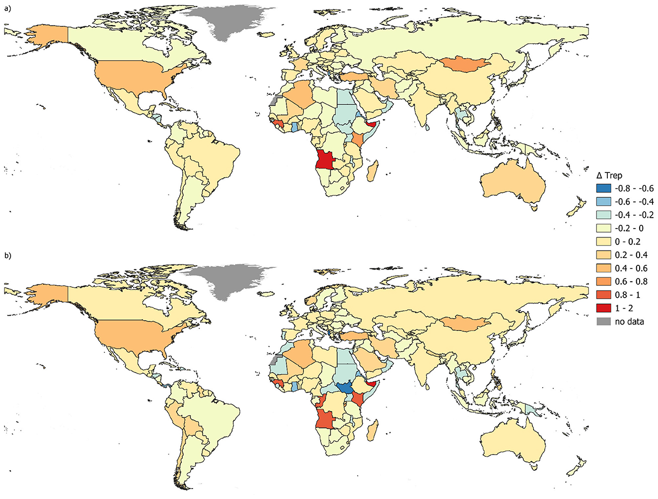
Figure 1. $\Delta T_{rep}^{pop}$ for tas (a) and tasmax (b) based on changes in population distribution between 1985 (1980–1989) and 2020 (2015–2024). Negative numbers indicate reduced heat exposure due to changes in population distribution, positive numbers indicate elevated heat exposure because of changes in population distribution in addition to climate in the same time period.

Figure 2

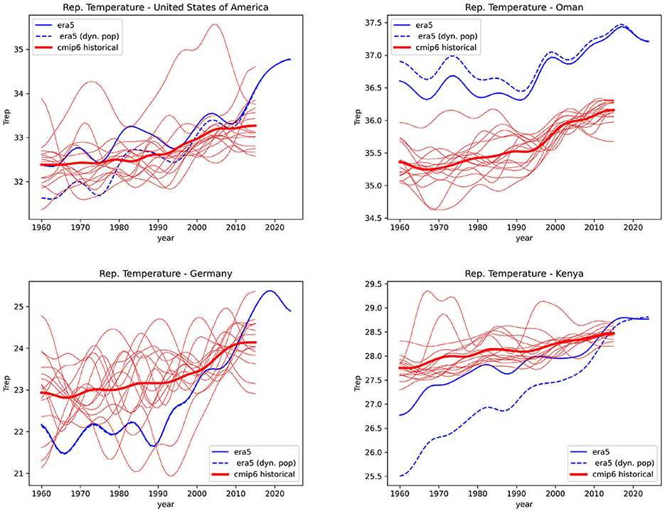
Figure 2. Curves for $T_{rep}^{tasmax}$ for the United States (top left), Oman (top right), Germany (bottom left), and Kenya (bottom right). The blue lines show the heat exposure based on ERA5 reanalysis data using either a static population scenario (solid line) or the dynamic population scenario (dashed). Red lines indicate CMIP6 historical baseline results considering a static population scenario. The strong red lines represent the ensemble mean of the individual simulations (thin red lines). Lines have been Gaussian smoothed (σ = 3 years) for better readability.

In countries with substantial population growth and urbanization dynamics, the locations where their populations settled strongly contributed to their overall heat exposure. For example, in the United States, as GHSL data show, relative population growth was strongest in Southern and Western states, which exhibit higher temperatures. This led to a contribution of about 26% to heat exposure due solely to changes in population patterns for both tasmax and tas statistics.

Urbanization can have a major impact on heat exposure, depending on where the urban centers of a country are located. In Norway, the concentration of a large proportion of the population in the Oslo region, which is warmer than most of the rest of the country, contributes about 60% of the positive change in heat exposure for tas. On the other hand, in countries like the United Arab Emirates or Oman, where their capitals are located in more temperate places than the rest of the country, the accumulation of population in these capitals reduces heat exposure in comparison to the static population scenario. This indicates that if these countries had had the population distribution of 2020 in earlier decades, their heat exposure would have been lower.

In summary, changes in spatial population distribution did contribute in many countries to a change in heat exposure. Across all countries, independent of whether changes in population distribution elevated or counter-acted temperature rise, population dynamics contributed about 17.5% to the observed climate change between 1960 and 2024. On average, it reduced the temperature increase, e.g., for tasmax by about 5% as migration to cooler areas within a country were more common. However, this does not necessarily indicate general reduction of heat exposure as e.g., effects of urban heat is not considered in this study. For the majority of countries, this contribution is minimal (e.g., Germany, +0.24%), while it can be substantial for others (e.g., Kenya +42% or Morocco –32%). Especially for countries with smaller populations, the accumulation of people due to urbanization can be a major driver for increasing or reducing heat exposure, on top of climate change impacts. In some cases, these contributions can be even larger than those from climate change or can completely counteract the signal. In addition, urbanization also leads to urban heat islands, which elevate heat exposure based on tas at a smaller regional resolution than that captured in this assessment.

4.2 Historical review of ERA5 and CMIP6

To accurately assess heat exposure for the upcoming decades under different climate pathways, it is necessary to assess the differences between observations and the underlying historical baseline of the applied CMIP6 models. The goal is to identify potential regional and temporal biases between the ERA5 reanalysis data, considered ground truth, and the CMIP6 ensemble. This is done by applying the static population model of 2020.

It should be noted that CMIP6 models generally exhibit systematic biases when compared to reanalysis datasets. Previous studies have shown that they often overestimate land surface temperatures, particularly in tropical and arid regions, while underestimating warming in high-latitude areas (Fan et al., 2020; Duan et al., 2025). Such discrepancies may lead to an overestimation or underestimation of heat exposure, depending on regional climate characteristics.

In our assessment, we compared T_rep for both tasmax and tas computed for the historical period (1960–2014) of CMIP6 and ERA5. The CMIP6 ensemble mean results show a mix of positive and negative biases compared to ERA5, which vary by region. In Eastern Europe (e.g., Ukraine, Romania, Slovakia, and Belarus), there is a large positive bias, suggesting an overestimation by CMIP6 in terms of heat exposure. Conversely, parts of Southeast Asia (Philippines, Sri Lanka, Indonesia, and Vietnam), parts of Scandinavia, and Central America show a negative bias, indicating an underestimation of temperatures. In addition, the largest errors were found for arid regions like Qatar, Kuwait, and Chile, where CMIP6 substantially underestimates the ERA5 values. These biases are found for both tas and tasmax. For T_rep based on daily maximum temperature, the biases were generally more pronounced, indicating an underestimation of extreme values.

Furthermore, we compared the last decade of observational data (2015–2024) with the corresponding first decade of the CMIP6 models under different potential pathways. Since these pathways are very close together in their initial years, we compared the difference between observations and the mean of SSP2-4.5 and SSP5-8.5 for that decade.

In general, most biases from the historical reference period remain consistent throughout these climate projections. In some places they are amplified, as in Armenia or Chile. In other places, a shift from underestimation to overestimation takes place, as in various European countries (e.g., Germany, Switzerland, France, and the United Kingdom). Especially, arid regions continue to show a consistent underestimation, while, e.g., Eastern Europe remains overestimated.

Warming of the last decade has been insufficiently captured in many places, as shown by the described error shift and the amplification of pre-existing underestimation. The global distribution of these biases can be seen in Figure 3, which highlights both historical and recent biases. Figure 2 also shows the variability of individual climate models, together with their ensemble mean, in comparison to ERA5 for selected countries. In summary, for the historical period, warming has been over- and underestimated in a roughly equal number of countries (about 35–40 each). For the remaining countries, a bias of less than 0.5°C is considered negligible. For the most recent decade (2015–2024), warming has been underestimated more frequently. A relevant overestimation was identified for tasmax in only 20 countries, while almost 70 countries can be considered underestimated. For tas, this bias is less pronounced.

Figure 3

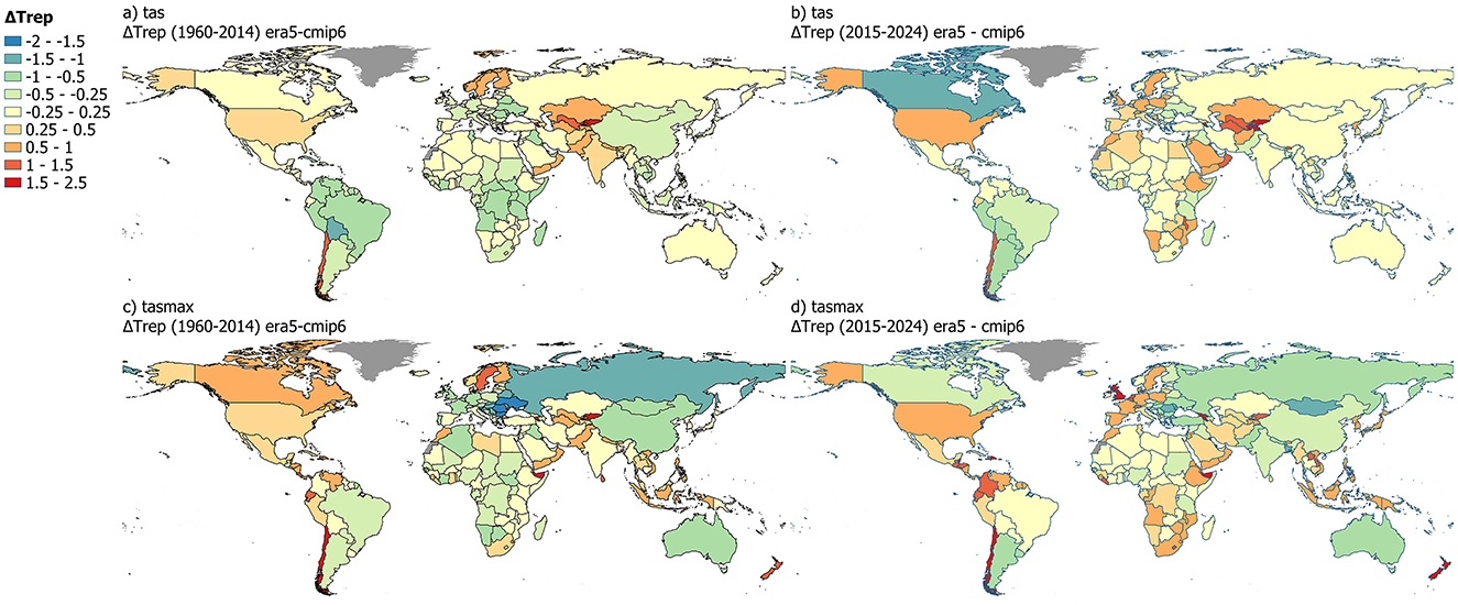
Figure 3. Absolute change of T_rep for tas (a) and tasmax (b) comparing the historic reference period (1960 to 2014) of ERA5 and the CMIP6 ensemble mean (a, c) and the difference between observed T_rep from the latest observational decade (2015–2024) compared to the first modeled decade of CMIP6 (b, d). Positive values indicate that the observed temperatures are higher than the model.

Since T_rep relies on an exponential weighting of temperatures, individual extreme values become more important compared to a long-term average. Individual extremes are often filtered out by averaging across different models, as is done here by computing the ensemble mean. This results in maximum temperature extremes being more likely to be missed than average temperatures. In addition, if a model bias occurs in densely populated regions, it becomes more pronounced due to the population weighting technique applied to retrieve T_rep.

4.3 Future climate

The final part of this analysis focuses on the upcoming decades to estimate how heat exposure might change and how such trends might be biased based on the lessons learned from the review of historical decades. Thus, we have assessed SSP2-4.5 and SSP5-8.5 until 2100 assuming a static population scenario. It is important to note that the influence of population dynamics is neglected due to a lack of sufficient future projections of population distribution. The influence of a changing population distribution would come on top.

Under this premise, we incorporate these biases into the bias indicator I, which considers biases resolved from both tas and tasmax. I is the sum on I_p, I_h and I_r based on tas and tasmax, respectively. Their threshold parameters have been set to t_p = 10% and t_h = t_r = 0.5, which are approximately the upper and lower sigma bounds based on the national statistics across all countries. Ranging from -6 to +6,a high value indicates a potential underestimation of heat exposure by the CMIP6 models, while low values indicate a potential overestimation. Figure 4 shows the global distribution of I, revealing some clear patterns. In case of I_p it is assumed that the population dynamics of the past decades are indicative for the population dynamics of future decades (e.g., continuous urbanization).

Figure 4

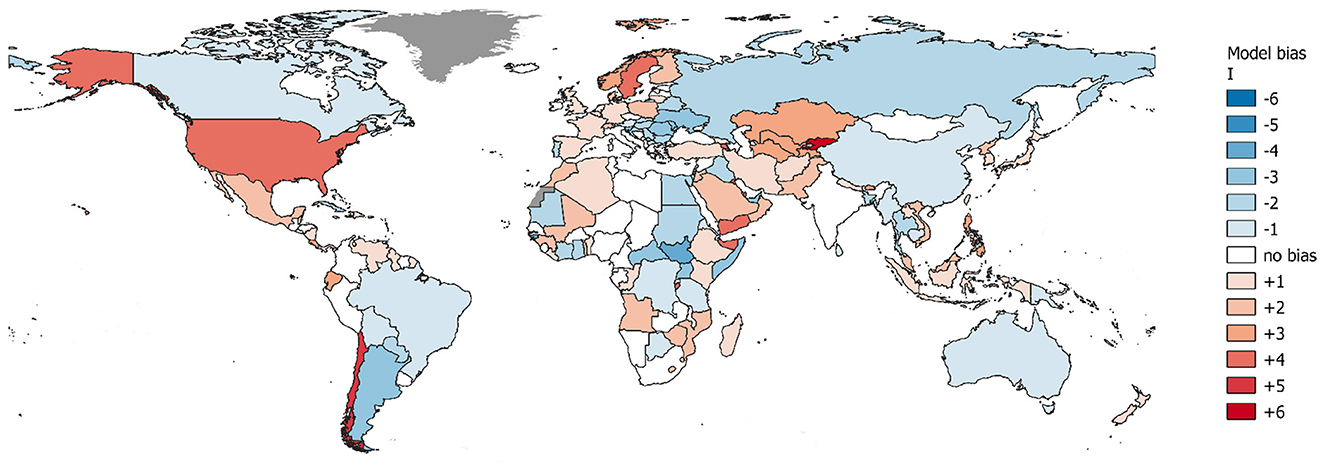
Figure 4. Model bias indicator I based on the combined observed biases from population distribution changes, and relative errors between ERA5 and CMIP6 from both historical and recent observation periods taking into account biases from both tas and tasmax. A high value indicates a potential underestimation of CMIP6 heat exposure, while a low values indicates a potential overestimation.

Most notably, parts of the Middle East, Central Asia, the Americas, and Northern Europe experience the strongest bias toward underestimation, including the United States (+4), Chile (+5), Yemen (+3), Sweden (+4), and Kyrgyzstan (+6). Generally, most of Western Europe sees a potential underestimation, while most of Eastern Europe, except for Poland and the Baltics, might be overestimated. Across Africa, the distribution is heterogeneous. Most countries along the Nile River may be overestimated, except for Ethiopia (+1). A similar pattern can be seen for the Central African countries, except for Burundi (+4) where heat exposure might be underestimated, especially in South Sudan (–4). In South America, countries East of the Andes show a tendency to be overestimated, while those West of the Andes are either neutral or potentially underestimated, especially Chile.

Such biases indicate challenges in properly representing regional climate dynamics in global models, particularly when also accounting for a granular human exposure in these places. Using a population-weighted approach in this study also ensures that desolate places without any exposure do not interfere with geospatial statistics. Thus, the observed biases are highly relevant for risk-driven assessments.

However, the most important question is what the future climate might look like. For this purpose, we compiled the change in T_rep for both tas and tasmax (denoted as ΔT_rep) for the period since 1980, as well as for future projections in the 2050s and 2090s for both SSP2-4.5 and SSP5-8.5 (Figures 5, 6). These projections indicate the most notable changes in heat exposure will be in Europe, especially in Eastern Europe, which could represent an overestimation according to the biases described above. On average, the trends for tasmax and tas are very similar in most countries. However, countries with high altitude, like Bolivia, or arid places with already high daily maximum temperatures, like Iraq, experience much more pronounced changes in their daily average temperatures than in their maximums. In addition, mid-latitude countries experience higher absolute and relative changes in their heat exposure than those in the tropics, where average daily temperatures are already high. Nonetheless, heat exposure from average and maximum daily temperatures increases in all countries and under both scenarios.

Figure 5

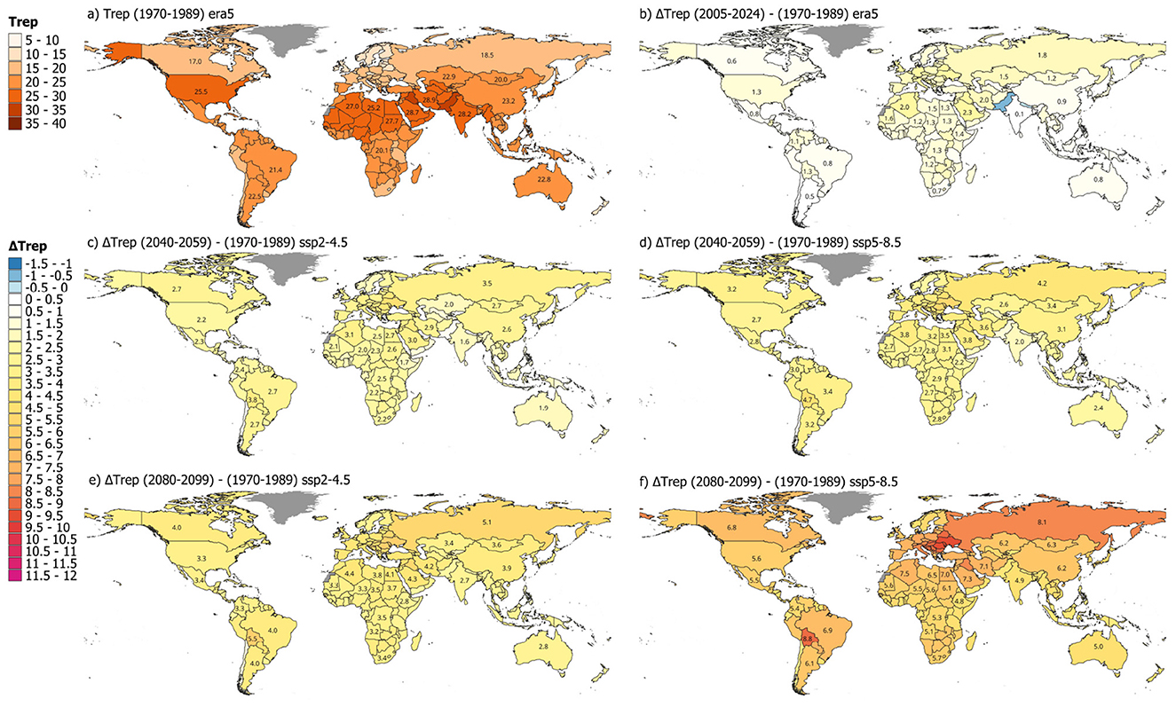
Figure 5. World view on T_rep based on tas in the 1980s (a) and its changes in ΔT_rep by 2020 (2015–2024) (b), and by 2050 for SSP2-4.5 (c) and SSP5-8.5 (d) and 2090s (e, f).

Figure 6

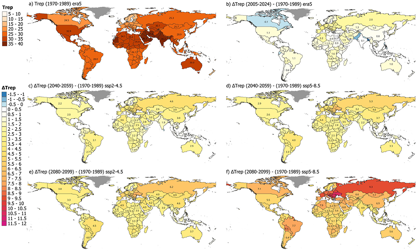
Figure 6. World view on T_rep based on tasmax in the 1980s (a) and its changes in ΔT_rep by 2020 (2015–2024) (b), and by 2050 for SSP2-4.5 (c) and SSP5-8.5 (d) and 2090s (e, f).

The changes in heat exposure inevitably go hand-in-hand with changes in climate zones (Cui et al., 2021). However, climate zones depend on more variables than just temperature and provide a good qualitative way to describe the climate or a part of it. Thus, we introduce so-called “heat zones” based on the average heat exposure from tas and tasmax, ${\overline{T}}_{rep}$, which is defined as

$\begin{array}{ll}{\overline{T}}_{rep}=\frac{(T_{rep}^{tas}+T_{rep}^{tasmax})}{2}& (10)\end{array}$

In total, we define eight different heat zones based on five-degree increments of ${\overline{T}}_{rep}$, which range from 5 to 45, covering cold, temperate, and warm climates with intermediate steps. The highest class, “unbearably warm,” had not manifested by 2020 but might occur by the 2050s under SSP5-8.5 or by the 2090s under SSP2-4.5 in the Middle East. Table 2 summarizes these different classes. These zones are based on qualitative descriptions, provided by the authors, of contemporary conditions in the respective countries (e.g., France) or in the places within those countries where the majority of people live (e.g., Canada). These zones can be considered a temperature- and population-weighted simplification of the Köppen climate classification. Cui et al. (2021) and Belda et al. (2014) have taken similar approaches. It should be remembered that these zones are based on population-weighted temperatures. In the case of the United States, California, Texas, and Florida, with their high populations, dominate the overall classification, in contrast to, e.g., Montana or Alaska, which have very few people.

Table 2

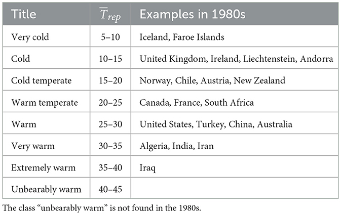
Table 2. Definition of heat zones based on ${\overline{T}}_{rep}$, which is the average of T_rep resolved from tas and tasmax.

The class “unbearably warm” was introduced to account for heat exposures not yet experienced today. Considering that heat is already substantially challenging for some societies today, a further increase in average and maximum temperatures can lead to a potentially unbearable situation where a region is no longer suitable to sustain human life.

Already by 2020, many countries had changed their heat zone since 1980. For example, Spain moved from a “warm temperate” to a “warm” country, while most of Central Europe increased from “cold temperate” to “warm temperate.” The movement of heat zones is illustrated both in Figure 7 as global maps and in Figure 8, which provides the distribution of all countries across heat zones. The latter highlights that countries classified as “very cold” or “cold” today may disappear as early as the 2050s or at the latest by the 2090s. “Warm temperate" countries are the most common class of heat exposure worldwide today. However, by the 2050s, “warm” countries will become the most common, and by the 2090s under SSP5-8.5, there will be more countries classified as “very warm” or above worldwide than in any other category. Between 1980 and 2020, about a third of all countries experienced an increase in their heat zone by one level. By 2050, under SSP5-8.5 (which is almost equivalent to 2090 under SSP2-4.5), only a third of the countries have not yet switched their heat zones, while a few countries have even moved a second level higher.

Figure 7

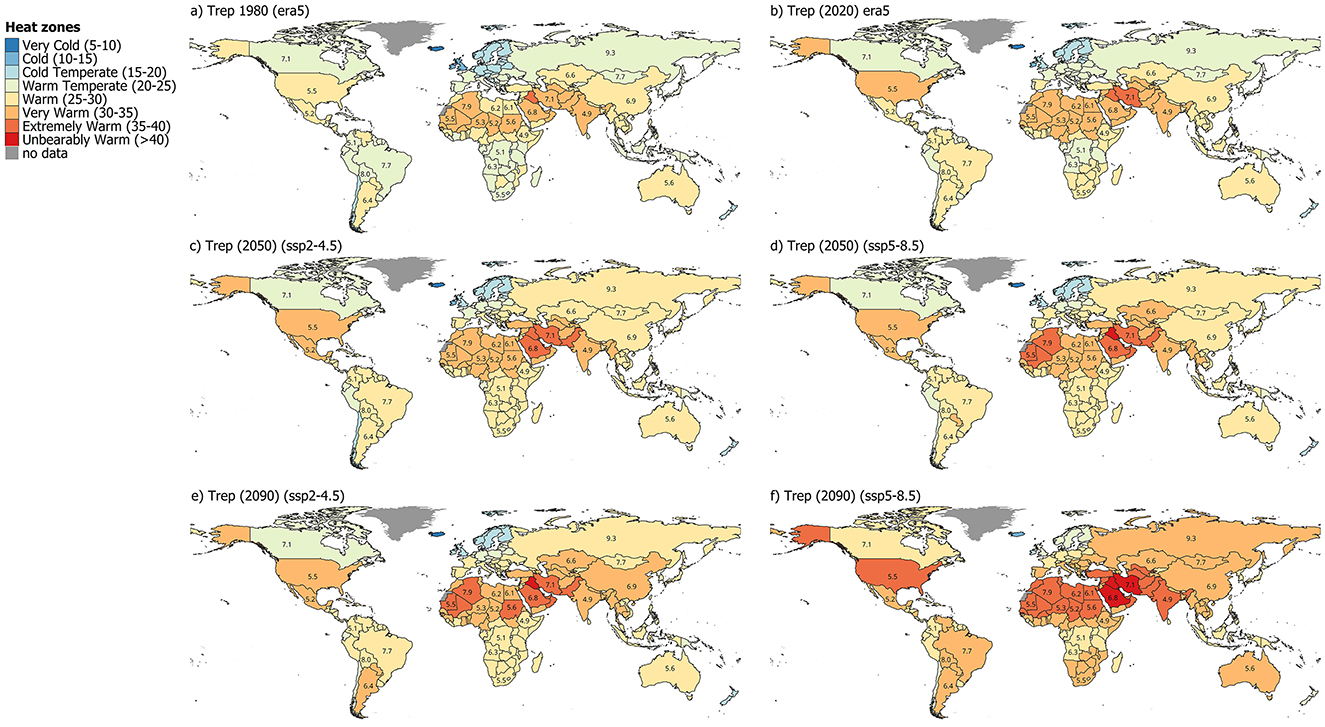
Figure 7. World view on different heat zones in 1980 (a), 2020 (b) and by 2050 for SSP2-4.5 (c) and SSP5-8.5 (d) and 2090 respectively (e, f).

Figure 8

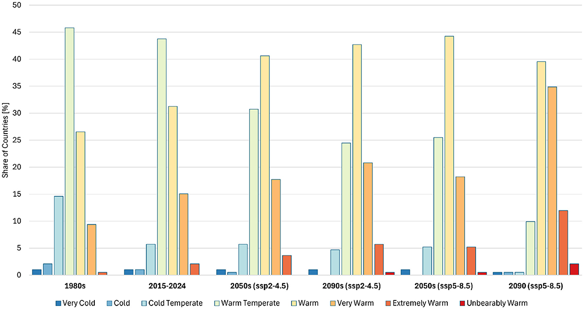
Figure 8. Histograms on the qualitative heat zones for different decades and climate projections showing the shift from a majority of cold and temperate countries to mostly warm.

5 Discussion

In our study, we have shown how population dynamics have influenced heat exposure in different countries, to what extent ERA5 and CMIP6 data fit together, and where potential errors and biases should be considered. Furthermore, we assessed what future heat exposure may look like and how it compares to today's situation using a qualitative classification system.

Overall, this assessment highlights the increasing heat exposure worldwide. Following the nomenclature of heat zones used in this study, the increase in countries experiencing “very warm” and “extremely warm” heat conditions, as well as the potential emergence of an “unbearably warm” zone, highlight the growing risk of extreme heat. The consequences can be severe with respect to heat-related mortality, impacts on agricultural productivity, and the potential for increased migration pressure. Several countries in regions already experiencing exceptionally high temperatures, such as the Middle East, Southeast Asia, or major parts of Africa, may move into extreme heat conditions as early as the 2050s. In addition, mid-latitude countries in regions such as Europe experience the largest increase in heat exposure.

Despite these overall trends, there are various biases and potential error sources that need to be addressed. First, the assessed climate projections rely on the latest CMIP6 climate models, which still contain various uncertainties and regional biases, as highlighted in the comparison with ERA5 for recent decades. Places that are highlighted by these models to experience some of the most pronounced changes in heat exposure, such as Eastern Europe, are also indicated to be constantly overestimated by the CMIP6 historical baseline, which counteracts the projected extremes.

In addition, this assessment was carried out on a country-by-country basis, where sub-national variations have only been considered by introducing a population-based weighting technique. However, for very large countries like the United States, Brazil, or India, this might still be insufficient. Future iterations of this research should take into account smaller administrative units.

Furthermore, as shown for recent decades, changes in population can significantly impact heat exposure, especially in countries with substantial dynamics in demography and spatial migration. Even though we have limited the analysis to a static population model after 2020, future migration patterns are very uncertain and will potentially be influenced by a changing climate itself (Balsari et al., 2020). Thus, as in the past, heat exposure also depends on where people decide to live in the future. This can also be connected to changes in land use, which also influence regional temperature patterns (Adeyeri et al., 2023). Additional improvements could be made considering also projections of population patterns into the future. However, this would also introduce further modeling uncertainties and assumptions which need to be addressed within the analysis.

Likewise, the effect of the urban heat island, which would have a substantial impact on daily average temperatures in urbanized regions, depends on the spatial distribution of settlements. This is especially important since urbanization is a key driver behind the demographic contribution to changes in heat exposure. In the future, higher-resolution climate models should be used to better capture heat distribution in general and, specifically, to better account for effects such as the urban heat island, in order to better quantify the actual burden of heat in cities.

Finally, this assessment is solely based on temperature to quantify heat exposure. However, in terms of heat risk to, for example, health, humidity is a crucial factor (Ebi et al., 2021). Hot temperatures in dry climates are less dangerous than those in more humid climates. Here, future research should also take into account heat based on indicators such as the heat index or humidex (Diaconescu et al., 2023).

6 Conclusion

The results of our study outline the significant shift in global temperatures that has already occurred and the expected intensification of these trends over the coming decades. However, it was also shown that climate change is not the only major driver of national heat exposure. Population dynamics with respect to changes in the relative population distribution within a country—for example, due to urbanization or conflicts—can substantially increase or reduce heat exposure over decades. This must be taken into account when planning climate adaptation measures at a national level. Habitability with respect to heat will become an increasingly important factor in international and domestic migration.

In addition, by providing a qualitative classification of heat exposure, it is easier to compare the level of heat today with that of tomorrow and to identify places where countermeasures are needed. For example, Germany should carefully review the heat adaptation measures used in the Mediterranean, as its future climate will be closely reminiscent of that in parts of Italy or France today. However, a spatially more granular approach at a sub-national or city level would provide even greater insight into such relationships.

Nonetheless, our results should be interpreted carefully due to the inherent biases and uncertainties from climate models, population dynamics (this study limited future population to a static distribution of 2020), and geospatial aggregation (linear interpolation of climate models). Countries with existing heat exposure will see exacerbated risks, while those previously considered temperate are entering new and unfamiliar climate regimes.

This study underlines the importance of integrating high-resolution climate and demographic data for more precise risk assessments. The underrepresentation of urban heat stress, regional feedback mechanisms, and socioeconomic vulnerabilities within future socioeconomic pathways suggests that actual exposure may be even higher than estimated. These findings recommend a more holistic approach to assessing the impacts and dynamics of heat exposure, one that integrates scientific perspectives from climate science, risk science, and health science, as well as from policymakers and urban planners. In addition, it might be help to also include other climate pathways, e.g., SSP1-2.6, which is more in-line with the Paris Agreement, to highlight what the best potential future among all pathways could be, despite becoming more unlikely.

The results of the current worst-case climate pathway, SSP5-8.5, highlight the crucial need to avoid a future where heat exposure becomes extreme for too many places in the world—a situation that would be potentially unbearable for many societies. Achieving a pathway similar to SSP2-4.5 would still be a challenge for many countries, requiring costly adaptation measures. However, the authors hope that the findings of this study support decision-makers in advancing climate mitigation and adaptation and motivate scientists to close the identified data and research gaps to better understand the impact dynamics of climate change.

Data availability statement

The raw data supporting the conclusions of this article will be made available by the authors, without undue reservation.

Author contributions

AS: Conceptualization, Formal analysis, Methodology, Writing – original draft, Writing – review & editing. PL: Conceptualization, Formal analysis, Writing – original draft, Writing – review & editing. SM: Supervision, Validation, Writing – review & editing. SK: Writing – original draft. BM: Conceptualization, Investigation, Writing – original draft. SB: Conceptualization, Writing – original draft. MK: Supervision, Writing – review & editing.

Funding

The author(s) declare that no financial support was received for the research and/or publication of this article.

Conflict of interest

The authors declare that the research was conducted in the absence of any commercial or financial relationships that could be construed as a potential conflict of interest.

Generative AI statement

The author(s) declare that no Gen AI was used in the creation of this manuscript.

Any alternative text (alt text) provided alongside figures in this article has been generated by Frontiers with the support of artificial intelligence and reasonable efforts have been made to ensure accuracy, including review by the authors wherever possible. If you identify any issues, please contact us.

Publisher's note

All claims expressed in this article are solely those of the authors and do not necessarily represent those of their affiliated organizations, or those of the publisher, the editors and the reviewers. Any product that may be evaluated in this article, or claim that may be made by its manufacturer, is not guaranteed or endorsed by the publisher.

References

Adeyeri, O. E., Zhou, W., Laux, P., Wang, X., Dieng, D., Widana, L. A., et al. (2023). Land use and land cover dynamics: Implications for thermal stress and energy demands. Renew. Sustain. Energy Rev. 179:113274. doi: 10.1016/j.rser.2023.113274

Crossref Full Text | Google Scholar

Adinolfi, M., Raffa, M., Reder, A., and Mercogliano, P. (2023). Investigation on potential and limitations of ERA5 Reanalysis downscaled on Italy by a convection-permitting model. Clim. Dyn. 61, 4319–4342. doi: 10.1007/s00382-023-06803-w

Crossref Full Text | Google Scholar

Bai, Y., Zhang, F., Ma, X., Ma, H., and Liu, Q. (2025). Enhancing crop yield predictions under drought: Integrating Accumulated Drought Degree Days into the WOFOST model. Ecol. Model. 508:111224. doi: 10.1016/j.ecolmodel.2025.111224

Crossref Full Text | Google Scholar

Ballester, J., Quijal-Zamorano, M., Méndez Turrubiates, R. F., Pegenaute, F., Herrmann, F. R., Robine, J. M., et al. (2023). Heat-related mortality in europe during the summer of 2022. Nat. Med. 29, 1857–1866. doi: 10.1038/s41591-023-02419-z

PubMed Abstract | Crossref Full Text | Google Scholar

Balsari, S., Dresser, C., and Leaning, J. (2020). Climate change, migration, and civil strife. Curr. Environ. Health Rep. 7, 404–414. doi: 10.1007/s40572-020-00291-4

PubMed Abstract | Crossref Full Text | Google Scholar

Belda, M., Holtanová, E., Halenka, T., and Kalvová, J. (2014). Climate classification revisited: from köppen to trewartha. Clim. Res. 59, 1–13. doi: 10.3354/cr01204

Crossref Full Text | Google Scholar

Cannon, A. J., Sobie, S. R., and Murdock, T. Q. (2015). Bias correction of gcm precipitation by quantile mapping: how well do methods preserve changes in quantiles and extremes? J. Clim. 28, 6938–6959. doi: 10.1175/JCLI-D-14-00754.1

Crossref Full Text | Google Scholar

Casanueva, A., Herrera, S., Iturbide, M., Lange, S., Jury, M., Dosio, A., et al. (2020). Testing bias adjustment methods for regional climate change applications under observational uncertainty and resolution mismatch. Atmosphere. Sci. Lett. 21:e978. doi: 10.1002/asl.978

Crossref Full Text | Google Scholar

Cui, D., Liang, S., and Wang, D. (2021). Observed and projected changes in global climate zones based on köppen climate classification. Clim. Change 12:e701. doi: 10.1002/wcc.701

Crossref Full Text | Google Scholar

Diaconescu, E., Sankare, H., Chow, K., Murdock, T. Q., and Cannon, A. J. (2023). A short note on the use of daily climate data to calculate humidex heat-stress indices. Int. J. Climatol. 43, 837–849. doi: 10.1002/joc.7833

Crossref Full Text | Google Scholar

Duan, L., Freese, L. M., Bala, G., and Caldeira, K. (2025). Historical model biases in monthly high temperature anomalies indicate under-estimation of future temperature extremes. Commun. Earth Environ. 6:604. doi: 10.1038/s43247-025-02579-5

Crossref Full Text | Google Scholar

Ebi, K. L., Capon, A., Berry, P., Broderick, C., de Dear, R., Havenith, G., et al. (2021). Hot weather and heat extremes: health risks. Lancet 398, 698–708. doi: 10.1016/S0140-6736(21)01208-3

PubMed Abstract | Crossref Full Text | Google Scholar

Ehret, U., Zehe, E., Wulfmeyer, V., Warrach-Sagi, K., and Liebert, J. (2012). Hess opinions “should we apply bias correction to global and regional climate model data?” Hydrol. Earth Syst. Sci. 16, 3391–3404. doi: 10.5194/hess-16-3391-2012

Crossref Full Text | Google Scholar

Eugenio Pappalardo, S., Zanetti, C., and Todeschi, V. (2023). Mapping urban heat islands and heat-related risk during heat waves from a climate justice perspective: a case study in the municipality of Padua (Italy) for inclusive adaptation policies. Landsc. Urban Plann. 238:104831. doi: 10.1016/j.landurbplan.2023.104831

Crossref Full Text | Google Scholar

Eyring, V., Bony, S., Meehl, G. A., Senior, C. A., Stevens, B., Stouffer, R. J., et al. (2016). Overview of the coupled model intercomparison project phase 6 (cmip6) experimental design and organization. Geosci. Model Dev. 9, 1937–1958. doi: 10.5194/gmd-9-1937-2016

Crossref Full Text | Google Scholar

Fan, X., Miao, C., Duan, Q., Shen, C., and Wu, Y. (2020). The performance of CMIP6 versus CMIP5 in simulating temperature extremes over the global land surface. J. Geophys. Res. Atmos. 125:e2020JD033031. doi: 10.1029/2020JD033031

Crossref Full Text | Google Scholar

Freire, S., MacManus, K., Pesaresi, M., Doxsey-Whitfield, E., and Mills, J. (2016). “Development of new open and free multi-temporal global population grids at 250 m resolution,” in Geospatial Data in a Changing World: Selected Papers of the 19th AGILE Conference on Geographic Information Science.

Google Scholar

Gallo, E., Quijal-Zamorano, M., Méndez Turrubiates, R. F., Tonne, C., Basaga na, X., Achebak, H., et al. (2024). Heat-related mortality in Europe during 2023 and the role of adaptation in protecting health. Nat. Med. 30, 3101–3105. doi: 10.1038/s41591-024-03186-1

PubMed Abstract | Crossref Full Text | Google Scholar

Gasparrini, A., Guo, Y., Hashizume, M., Kinney, P. L., Petkova, E. P., Lavigne, E., et al. (2015). Mortality risk attributable to high and low ambient temperature: a multicountry observational study. Lancet 386, 369–375. doi: 10.1016/S0140-6736(14)62114-0

PubMed Abstract | Crossref Full Text | Google Scholar

Hersbach, H., Bell, B., Berrisford, P., Hirahara, S., Horányi, A., Muñoz-Sabater, J., et al. (2020). The era5 global reanalysis. Q. J. R. Meteorol. Soc. 146, 1999–2049. doi: 10.1002/qj.3803

Crossref Full Text | Google Scholar

Holmer, B., and Eliasson, I. (1999). Urban-rural vapour pressure differences and their role in the development of urban heat islands. Int. J. Climatol. 19, 989–1009. doi: 10.1002/(SICI)1097-0088(199907)19:9<989::AID-JOC410>3.0.CO;2-1

Crossref Full Text | Google Scholar

Hooyberghs, H., Verbeke, S., Lauwaet, D., Costa, H., Floater, G., and De Ridder, K. (2017). Influence of climate change on summer cooling costs and heat stress in urban office buildings. Clim. Change 144, 721–735. doi: 10.1007/s10584-017-2058-1

Crossref Full Text | Google Scholar

Huang, W. T. K., Braithwaite, I., Charlton-Perez, A., Sarran, C., and Sun, T. (2022). Non-linear response of temperature-related mortality risk to global warming in England and Wales. Environ. Res. Lett. 17:034017. doi: 10.1088/1748-9326/ac50d5

Crossref Full Text | Google Scholar

Hundhausen, M., Feldmann, H., Laube, N., and Pinto, J. G. (2023). Future heat extremes and impacts in a convection-permitting climate ensemble over germany. Nat. Haz. Earth Syst. Sci. 23, 2873–2893. doi: 10.5194/nhess-23-2873-2023

Crossref Full Text | Google Scholar

Jones, B., O'Neill, B., McDaniel, L., McGinnis, S., Mearns, L., and Tebaldi, C. (2015). Future population exposure to us heat extremes. Nat. Clim. Chang. 5, 652–655. doi: 10.1038/nclimate2631

Crossref Full Text | Google Scholar

Kjellstrom, T., Freyberg, C., Lemke, B., Otto, M., and Briggs, D. (2018). Estimating population heat exposure and impacts on working people in conjunction with climate change. Int. J. Biometeorol. 62, 291–306. doi: 10.1007/s00484-017-1407-0

PubMed Abstract | Crossref Full Text | Google Scholar

Klimiuk, T., Ludwig, P., Sanchez-Benitez, A., Goessling, H. F., Braesicke, P., and Pinto, J. G. (2024). The european summer heatwave 2019-a regional storyline perspective. Earth Syst. Dyn. Disc. 2024, 1–24. doi: 10.5194/esd-2024-16

Crossref Full Text | Google Scholar

Kosatsky, T. (2005). The 2003 european heat waves. Eurosurveillance 10, 3–4. doi: 10.2807/esm.10.07.00552-en

PubMed Abstract | Crossref Full Text | Google Scholar

Lo, Y. E., Mitchell, D. M., Buzan, J. R., Zscheischler, J., Schneider, R., Mistry, M. N., et al. (2023). Optimal heat stress metric for modelling heat-related mortality varies from country to country. Int. J. Climatol. 43, 5553–5568. doi: 10.1002/joc.8160

PubMed Abstract | Crossref Full Text | Google Scholar

Marx, W., Haunschild, R., and Bornmann, L. (2021). Heat waves: a hot topic in climate change research. Theor. Appl. Climatol. 146, 781–800. doi: 10.1007/s00704-021-03758-y

PubMed Abstract | Crossref Full Text | Google Scholar

Matthews, T., Wilby, R. L., and Murphy, C. (2017). Communicating the deadly consequences of global warming for human heat stress. Proc. Nat. Acad. Sci. 114, 3861–3866. doi: 10.1073/pnas.1617526114

PubMed Abstract | Crossref Full Text | Google Scholar

Mora, C., Dousset, B., Caldwell, I., Powell, F., Geronimo, R., Bielecki, C., et al. (2017). Global risk of deadly heat. Nat. Clim. Chang. 7, 501–506. doi: 10.1038/nclimate3322

Crossref Full Text | Google Scholar

Mourshed, M. (2012). Relationship between annual mean temperature and degree-days. Energy Build. 54, 418–425. doi: 10.1016/j.enbuild.2012.07.024

Crossref Full Text | Google Scholar

Muthers, S., Laschewski, G., and Matzarakis, A. (2017). The summers 2003 and 2015 in south-west germany: heat waves and heat-related mortality in the context of climate change. Atmosphere 8:224. doi: 10.3390/atmos8110224

Crossref Full Text | Google Scholar

Nogueira, M., Hurduc, A., Ermida, S., Lima, D. C. A., Soares, P. M. M., Johannsen, F., et al. (2022). Assessment of the Paris urban heat island in ERA5 and offline SURFEX-TEB (v8.1) simulations using the METEOSAT land surface temperature product. Geosci. Model Dev. Disc. 15, 5949–5965. doi: 10.5194/gmd-15-5949-2022

Crossref Full Text | Google Scholar

O'Neill, B. C., Tebaldi, C., van Vuuren, D. P., Eyring, V., Friedlingstein, P., Hurtt, G., et al. (2016). The scenario model intercomparison project (scenariomip) for cmip6. Geosci. Model Dev. 9, 3461–3482. doi: 10.5194/gmd-9-3461-2016

Crossref Full Text | Google Scholar

Riahi, K., van Vuuren, D. P., Kriegler, E., Edmonds, J., O'Neill, B. C., Fujimori, S., et al. (2017). The shared socioeconomic pathways and their energy, land use, and greenhouse gas emissions implications: an overview. Global Environ. Change 42, 153–168. doi: 10.1016/j.gloenvcha.2016.05.009

Crossref Full Text | Google Scholar

Rohat, G., Flacke, J., Dosio, A., Dao, H., and van Maarseveen, M. (2019). Projections of human exposure to dangerous heat in african cities under multiple socio-economic and climate scenarios. Earth's Fut. 7, 528–546. doi: 10.1029/2018EF001020

Crossref Full Text | Google Scholar

Saeed, S., Waqas, A., Xiang, J., and Cao, C. (2021). Energy implications of future heatwaves: a global review. Renew. Sustain. Energy Rev. 150:111473.

Google Scholar

Schiavina, M., Freire, S., Carioli, A., and MacManus, K. (2023). “Ghs-pop r2023a-ghs population grid multitemporal (1975–2030),” in European Commission (Joint Research Centre (JRC)).

Google Scholar

Schwingshackl, C., Hirsch, A. L., Sillmann, J., and Gudmundsson, L. (2021a). Heat stress indicators in cmip6: estimating future trends and thresholds. Environ. Res. Lett. 16:064036. doi: 10.1029/2020EF001885

Crossref Full Text | Google Scholar

Semenza, J. C., and Menne, B. (2009). Climate change and infectious diseases in europe. Lancet Infect. Dis. 9, 365–375. doi: 10.1016/S1473-3099(09)70104-5

Crossref Full Text | Google Scholar

Sherwood, S. C., and Huber, M. (2010). Adaptability limits to climate change due to heat stress. Proc. Nat. Acad. Sci. 107, 9552–9555. doi: 10.1073/pnas.0913352107

Crossref Full Text | Google Scholar

Szewczyk, W., Mongelli, I., and Ciscar, J.-C. (2021). Heat stress, labour productivity and adaptation in europe–a regional and occupational analysis. Environ. Res. Lett. 16:105002. doi: 10.1088/1748-9326/ac24cf

Crossref Full Text | Google Scholar

Thrasher, B., Wang, W., Michaelis, A., Melton, F., Lee, T., and Nemani, R. (2022). NASA global daily downscaled projections, CMIP6. Sci. Data 9:262. doi: 10.1038/s41597-022-01393-4

PubMed Abstract | Crossref Full Text | Google Scholar

Voogt, J. A., and Oke, T. R. (2003). Thermal remote sensing of urban climates. Rem. Sens. Environ. 86, 370–384. doi: 10.1016/S0034-4257(03)00079-8

Crossref Full Text | Google Scholar

Zhao, M., Lee, J. K. W., Kjellstrom, T., and Cai, W. (2021). Assessment of the economic impact of heat-related labor productivity loss: a systematic review. Clim. Change 167:22. doi: 10.1007/s10584-021-03160-7

Crossref Full Text | Google Scholar

Zhou, D., Xiao, J., Bonafoni, S., Berger, C., Deilami, K., Zhou, Y., et al. (2018). Satellite remote sensing of surface urban heat islands: progress, challenges, and perspectives. Rem. Sens. 11:48. doi: 10.3390/rs11010048

Crossref Full Text | Google Scholar