Techno-economic analysis of ocean iron fertilization

This study provides an updated, comprehensive framework for conducting a techno-economic assessment (TEA) of novel carbon dioxide removal approaches. Specifically, the framework is applied to a scenario involving ocean iron fertilization (OIF) in the Southern Ocean. The study investigates whether cost elements, such as administrative and support labor, are accurately included in standard methodologies and proposes solutions for characterizing prospective cost elements and uncertainty in novel CDR TEAs. The first-of-a-kind (FOAK) levelized cost of carbon (LCOC) for OIF deployment is approximately $200 per tonne of CO₂. Learning rates are applied, and prospective nth-of-a-kind (NOAK) costs decrease to approximately $180 per tonne of CO₂. A local sensitivity analysis indicates that oceanographic parameters, such as the export efficiency of carbon biomass to the deep ocean, have a greater impact on the LCOC compared to engineering parameters like the cost of equipment or materials. Nevertheless, large capital engineering expenditures of approximately $120–160 million also significantly affect the levelized cost. The effect of these high-impact parameters on the LCOC is demonstrated by a cost range from $25 per tonne of CO₂ to $53,000 per tonne of CO₂ for best- to worst-case scenarios when varying values for monitoring, reporting, and verification (MRV) processes, losses due to nutrient robbing, equivalent carbon (CO₂e) losses from N₂O production, CO₂ ventilation losses to the atmosphere, net increase in primary production, and export efficiency are considered. Additionally, the effect of learning rates on determining prospective costs is shown through a sensitivity analysis to have a less significant impact on the overall costs of deployment and, in turn, future cost reductions when large parameter input uncertainties are present. Based on these results, it is recommended that oceanographic parameters be better characterized through additional research and development to reduce uncertainty in cost estimation. Methods of OIF deployment, including MRV processes, should also be investigated to minimize capital costs. Additionally, the proposed framework, including the bottom-up business cost analysis, should be applied to other CDR approaches to provide consistent and comprehensive comparisons for companies and decision-makers, underpinning informed funding decisions in the CDR space.

1 Introduction

The cost of mitigating climate change is variable and uncertain and largely depends on the fractional mix of emissions reductions, carbon capture and storage (CCS), and carbon dioxide removal (CDR). To combat climate change and limit the global temperature rise to well below the target of 2°C outlined in the 2015 Paris Climate Agreement (Allen et al., 2018), removing and storing atmospheric carbon dioxide (CO₂) will be essential and will require the development of CDR strategies. Since the ocean currently absorbs about a third of anthropogenic CO₂ emissions and accounts for the majority of Earth’s natural carbon sequestration capacity (Buesseler et al., 2022; National Academies of Sciences Engineering and Medicine, 2022), there may be potential for additional CO₂ removal through ocean-based carbon dioxide removal (OCDR), commonly known as marine CDR (mCDR). Ocean-based approaches typically fall into two main categories: biotic approaches that utilize biomass generation or storage and abiotic approaches that involve adding materials such as rocks, minerals, and solutions to alter ocean carbonate chemistry (National Academies of Sciences Engineering and Medicine, 2022). Physical processes, such as artificial upwelling or downwelling, incorporating both biotic (upwelling/fertilization) and abiotic (downwelling of inorganic carbon to depths) elements (National Academies of Sciences Engineering and Medicine, 2022), could also be classified as a third intermediary category.

One potentially low-cost biotic approach is ocean nutrient fertilization, which involves adding macronutrients (nitrogen, phosphorus, and silicon), micronutrients (iron), or a combination of both to nutrient-deficient areas of the ocean (Yoon et al., 2018; National Academies of Sciences Engineering and Medicine, 2022). The increased concentration of these elements, crucial for phytoplankton growth, leads to a rise in the amount of photosynthetic carbon in the surface ocean, which reduces the fraction of dissolved carbon dioxide in seawater and drives additional atmospheric CO₂ uptake (National Academies of Sciences Engineering and Medicine, 2022). For this approach to effectively contribute to long-term carbon storage, organic carbon must sink into the deeper ocean (Bertram, 2011; National Academies of Sciences Engineering and Medicine, 2022; Bach et al., 2023).

Between 1993 and 2012, 14 artificial and 6 natural ocean trials were conducted on ocean iron fertilization (OIF) to examine the effects of both human and natural iron additions to the ocean (Williamson et al., 2012; Yoon et al., 2018; Boettcher et al., 2019; Kim, 2020; Buesseler et al., 2022). Iron acts as a limiting nutrient in various ocean ecosystems, and its addition enhances phytoplankton primary productivity. However, uncertainties remain regarding the fractional export of carbon to the deep ocean, the stability of the exported carbon, and the cost of carbon removal through this process (Williamson et al., 2012; Yoon et al., 2018; National Academies of Sciences Engineering and Medicine, 2022).

The variability in process conditions, as well as in background assumptions and methods employed, adds to the variability in cost estimates for ocean iron fertilization (OIF). As a result, it is difficult to compare cost estimates directly for such mCDR approaches. Cost estimates for ocean iron fertilization vary greatly, ranging from ~$2 to ~$1,280 per tonne of CO₂ removed (Boyd, 2008; Harrison, 2013; Babakhani et al., 2022; Bach et al., 2023; Emerson et al., 2024). Additional variance can arise from the inclusion of specific costs within economic models, such as labor, monitoring, reporting, and verification (MRV) processes, as well as deployment methods (e.g., aerial vs. ship-based). Monitoring costs include the expenses associated with collecting and storing data that demonstrates CO₂ removal is occurring (carbon tracking) while ensuring that negative environmental and ecological impacts are not occurring. This can be carried out through ocean sampling on dedicated research (MRV) vessels, the operation of autonomous underwater vehicles (AUVs), and recording the ocean’s surface via satellite. Reporting and verification costs include the expenses of generating carbon credits based on the collected data and having them verified by an independent third party.

Conventional techno-economic analysis (TEA) utilizes various methods to determine the costs of industrial processes, which have known inputs and outputs and exist in specific configurations. However, novel carbon dioxide removal (CDR) approaches that are in the early stages may be subject to substantial development, such that early configurations are simplifications of what is eventually deployed. The context in which these approaches are deployed, such as energy costs or climate policy, may also have greatly changed. Alternative frameworks for performing TEA on early-stage technologies have been proposed to address such concerns, such as the hybrid method (Rubin, 2019). This approach estimates the costs of a commercial first-of-a-kind (FOAK) process under the current context and process configurations, using bottom-up engineering cost estimation and applying learning rates to determine the nth-of-a-kind (NOAK) future (prospective) costs of a mature process. In this study, the FOAK process is an ocean iron fertilization (OIF) deployment at a technology readiness level (TRL) of 9, indicating a commercial operation that has been proven to work in the chosen environment (Rackley, 2023). The NOAK process is an OIF deployment at a TRL of 9 or more, indicating a mature commercial operation that has integrated with systems/value chains, achieved cost reductions due to learning, and undergone predictable growth (van der Spek et al., 2017; International Energy Agency, 2024). Conventional and hybrid cost estimation frameworks can be applied to early-stage technologies, but they have rarely been applied to CDR approaches such as OIF. As a result, there is a lack of comprehensive TEA case studies within the marine CDR (mCDR) space. Investigation of the applicability of conventional methodologies and their assumptions, as well as characterization of mCDR-specific aspects such as vessel maintenance costs and ocean monitoring, reporting, and verification (MRV), is essential to fill this research gap. Therefore, a comprehensive framework for prospective techno-economic analysis is proposed and applied to a case study of ocean iron fertilization. A sensitivity analysis of a selection of key input variables is undertaken to characterize uncertainty within the proposed TEA framework and provide suggestions on how to manage inherent uncertainty. The TEA is both prospective and ex ante, as it considers the future costs of an early-stage technology (Arvidsson et al., 2024).

2 Materials and methods

2.1 Framework for CDR

This study aims to inform future research and development (R&D) of ocean iron fertilization (OIF) as a carbon dioxide removal (CDR) strategy through a prospective techno-economic analysis of future deployment scenarios. Conventional cost methodologies from the U.S. Department of Energy’s National Energy Technology Laboratory (DOE/NETL) (Rubin et al., 2013; Theis, 2021; Henry et al., 2023) and the International Energy Agency Greenhouse Gas Programme (IEAGHG) (Rubin et al., 2013) were employed alongside an updated TEA framework to estimate the capital expenditure (CAPEX), operating expenditure (OPEX), cash flow, and economic indicators of a 28-year OIF project (3 years of construction, 25 years of deployment). The proposed OIF approach was divided into four stages: material production, transport of materials to the ocean, operation of the CDR approach, and monitoring, reporting, and verification (MRV), as recommended by Ward et al. (2024). The stage-by-stage structure, including the flow of materials and energy into and out of the process, is illustrated in Figure 1. It was assumed that multiple vessels equipped with mixing processes and storage tanks would deploy an acidified iron sulfate solution into the ocean to promote additional phytoplankton growth. The study uses OIF as a case study to evaluate the proposed TEA framework.

Figure 1

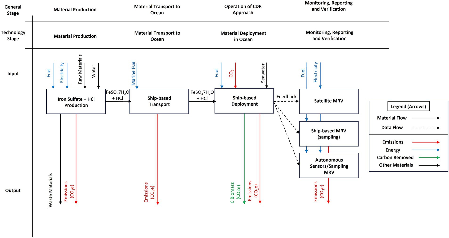
Figure 1. Overview of OIF process stages. Adapted from Ward et al. (2024).

2.2 Barriers to OIF implementation

A detailed analysis of the environmental impacts of OIF deployment is outside the scope of this study but must be conducted should this technology be considered for implementation. This includes aspects such as, but not limited to, the production of gases from phytoplankton growth and decay [dimethylsulfide (DMS), nitrous oxide (N2O)] (Williamson et al., 2012), nutrient robbing (the use of nutrients in OIF instead of natural biomass production/carbon uptake) (Buesseler et al., 2022; National Academies of Sciences Engineering and Medicine, 2022), mid- to deep-ocean anoxia or hypoxia (Gnanadesikan et al., 2003; Aumont and Bopp, 2006), deep-ocean acidification (due to enhanced carbon export from the surface ocean) (Oschlies et al., 2010; Buesseler et al., 2022), and disruption of ecosystem balance (Williamson et al., 2012; Buesseler et al., 2022). OIF has the potential to disrupt the ocean’s natural biological carbon pump and negatively affect existing ecosystems. Therefore, thorough life cycle assessments (LCAs) and studies on the wider impacts of OIF are essential. Pilot and demonstration work should incorporate best-practice guidance for responsible research and innovation [e.g., mCDR codes of conduct (Boettcher et al., 2023)]. It is crucial to incorporate the precautionary principle to balance the potential positive environmental benefits of OIF deployment to mitigate climate change against the associated negative environmental impacts (Güssow et al., 2010; Williamson et al., 2012).

It is assumed that a broader scientific foundation has been established prior to the implementation of OIF in this study, as the technology will be at a mature technology readiness level (TRL ~ 9). This includes the effects of OIF deployment on natural CDR (e.g., related to nutrient robbing) and broader environmental/ecosystem impacts. This would involve collaboration among marine biologists, ecologists, and the wider scientific community. Scientific knowledge should be developed to the point where verifiable computer modeling of OIF applications (carbon tracking and environmental impacts), with input from oceanic measurements, can accurately predict the long-term impacts of the process and comply with carbon accounting standards (Gnanadesikan et al., 2003; Bach et al., 2023). The costs of including this R&D were not factored into the cost estimate directly, as this case study presents the deployment costs in a future scenario where OIF is a more mature CDR approach. The pathway to achieving this deployment stage through R&D must be navigated before any large-scale commercial deployments occur. This ensures that ecological, ethical, and legal barriers to OIF implementation are only addressed once the necessary scientific foundation has been established.

Ocean Iron Fertilization (OIF) is a controversial carbon dioxide removal (CDR) approach, and its perceived public and political acceptability has led to legal restrictions that limit its deployment (Yoon et al., 2018; Bindoff et al., 2022; National Academies of Sciences Engineering and Medicine, 2022; Buesseler et al., 2024). Legal obligations regarding the spreading of fertilizing materials across the ocean must be addressed in the context of the London Convention, the London Protocol and the United Nations Convention on Biological Diversity (Kim, 2020) before OIF can be deployed at the scales discussed here. Since the scientific basis for OIF was assumed to have been developed prior to any deployment, the legal restrictions concerning OIF—specifically the London Convention and the London Protocol, which prevent large-scale OIF deployments—were also assumed to no longer be binding for the selected location of this study (Yoon et al., 2018; Bach et al., 2023). This assumption, which is inherently essential to any OIF deployment scenario, would require extensive work to be established and, therefore, should be specified whenever the costs from this study are applied elsewhere. The selected area is also outside the Commission for the Conservation of Antarctic Marine Living Resources (CCAMLR) marine protected area and the Antarctic Treaty zones, which aim to protect marine life and the Antarctic more generally (Bach et al., 2023). Thus, it was assumed that the process would not be subject to these regulations, which could hinder OIF deployment. Additional legal aspects were not considered, except for the inclusion of labor costs for operational legal expertise within the bottom-up business costing.

2.3 Location

The location of an OIF deployment is key to ensuring that carbon is removed, exported to deep waters, and durably sequestered for long time scales (>100 years) (Yoon et al., 2018; Kim, 2020; National Academies of Sciences Engineering and Medicine, 2022). An area of 200,000 km² was assumed to be fertilized in 90 parallel tracks with 5 km spacing, according to the scale suggested by previous cost estimates (Emerson et al., 2024).

The geographic location of the base case scenario was selected based on multiple criteria, including exclusion from countries’ exclusive economic zones (EEZ), exclusion from marine protected areas, proximity to downwelling/cold deep water in the global ocean conveyor belt, surface seawater temperatures sufficient for phytoplankton growth, availability of photosynthetically active radiation, high levels of surface nitrate and silicate, and low levels of surface iron and chlorophyll. These parameters were compared using graphs and diagrams from various sources (Boyd et al., 2007; Toulza et al., 2012; White and Costello, 2014; Yoon et al., 2018; National Academies of Sciences Engineering and Medicine, 2022; Encyclopædia Britannica, 2024) as well as the Ocean Visions online Ocean Iron Fertilization Site Suitability Planning Tool (Ocean Visions, 2024). The location was chosen to ensure the highest effectiveness possible across all categories (Figure 2). Exclusion from countries’ EEZs ensures that technology deployment occurs only with international agreements.

Figure 2

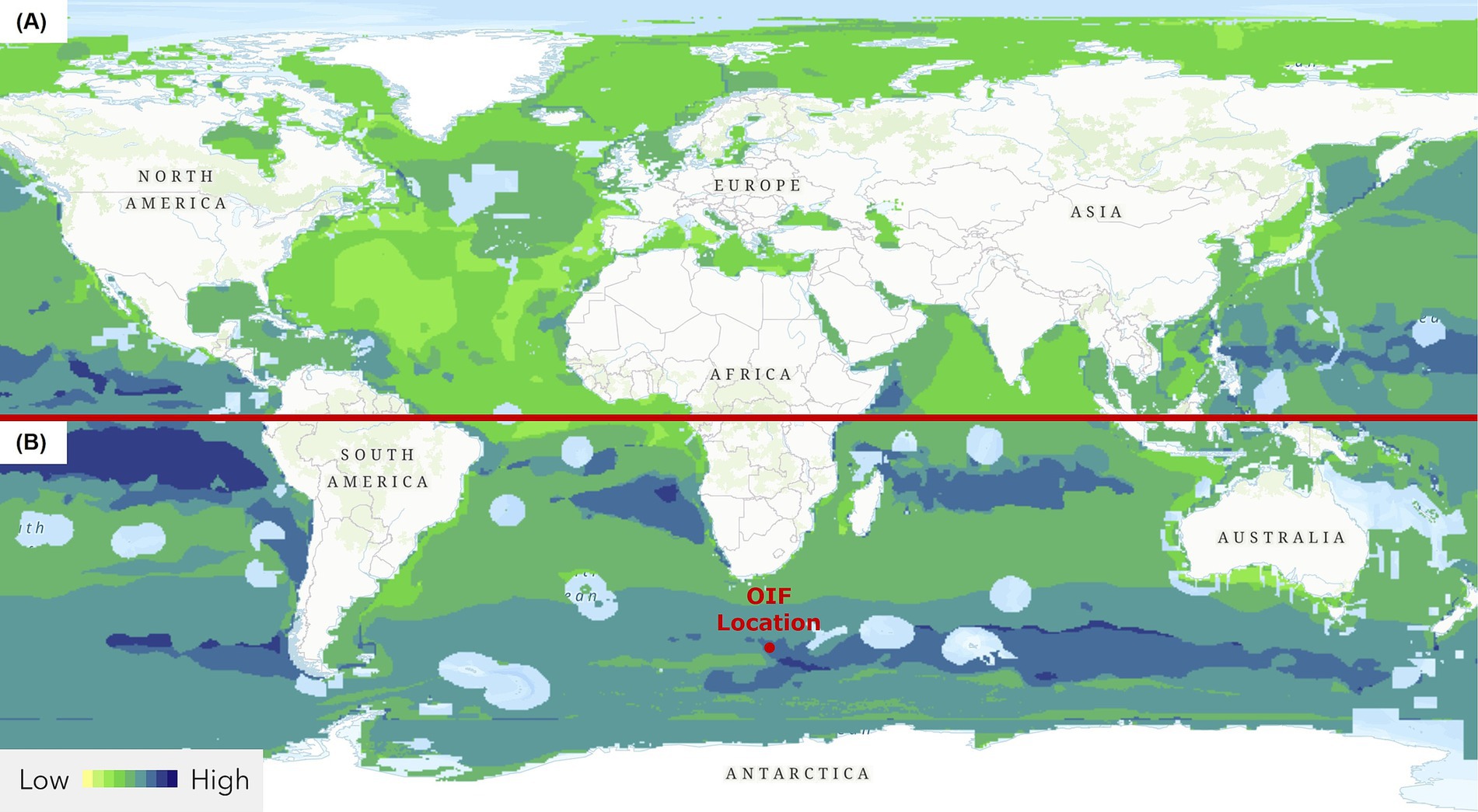
Figure 2. OIF case study locations. This map illustrates the proposed case study location (red dot) in relation to the distribution of OIF site suitability, adapted from Ocean Visions (2024). (A) depicts OIF site suitability during Northern Hemisphere summer conditions (April–September). (B) illustrates OIF site suitability in Southern Hemisphere summer conditions (October–March). Darker areas indicate greater suitability for OIF, considering factors such as the availability of photosynthetically active radiation, sea surface temperature, sea/air CO₂ exchange efficiency, upper ocean dissolved iron concentrations, upper ocean nitrate concentrations, and the presence of marine protected areas (shown as pale blue).

The OIF deployment location is situated off the coast of Antarctica (~1800 km from the port of Cape Town) and is close to the Southern Ocean (Figure 2). It is close to the deployment zone for a prior OIF field experiment known as EIFEX, which was the only previous OIF experiment to document a significant increase in the export of biomass (Yoon et al., 2018). Ports were chosen to align with major shipping routes (Rodrigue, 2017), aiming to minimize costs by utilizing the existing setup of the shipping sector.

2.4 Material and energy flows

An acidified iron sulfate solution comprised of iron sulfate heptahydrate (FeSO₄·7H₂O), 30 wt% hydrochloric acid (HCl), and seawater was utilized as the fertilizing material, as evidenced by its performance in ship-based OIF trials (Yoon et al., 2018; Emerson et al., 2024). Other materials, such as ferric chloride, have been proposed (Markels et al., 2011). However, their consideration fell outside the scope of this study since they have not been tested in field experiments.

The mass of iron required to achieve a specific concentration of iron on the ocean surface, the amount of carbon biomass produced and exported for storage in the deep ocean, and the net carbon removal were determined using the method provided by Emerson et al. (2024). The net carbon removal accounts for equivalent carbon (CO₂e) losses from nitrous oxide (N₂O) production, ventilation of remineralized CO₂ during and after the sinking of biomass (phytoplankton), and emissions from each process stage. The equivalent CO₂ (CO₂e) emission factors for the production of iron sulfate (0.200 tCO₂e/t FeSO₄·7H₂O) and hydrochloric acid (0.517 tCO₂e/t HCl) were estimated based on Emerson et al. (2024) and Ecoinvent LCI data (modeled with the IPCC 2021 LCIA method GWP 100), respectively. Emissions from the use of marine diesel oil (MDO) across all process stages were determined from a report by the International Maritime Organization (3.206 kgCO_2/kg MDO) (Faber et al., 2020).

The desired iron concentration in the ocean to stimulate phytoplankton growth (0.6 nmol/L) was estimated to be higher than in previous OIF experiments (~1.0–4.0 nmol/L) to ensure maximum growth rates for various species (Yoon et al., 2018; Emerson et al., 2024). The net increase in carbon production (~1,000 mg C/m²/day) and the growth phase of the bloom (~20 days) were informed by OIF experiments (Yoon et al., 2018; Emerson et al., 2024). The iron bioavailability fraction (the amount of iron available for use by phytoplankton) (Fe_av) was estimated at 20% of the added iron sulfate. Some studies indicated that between ~4% (Tsumune et al., 2005) and 24% (de Baar et al., 2005) of dissolved iron is available for biological uptake, while previous cost analyses have used values as high as 67% (Emerson et al., 2024). The concentration of iron in the product solution was specified at 0.5 M based on earlier OIF experiments (Martin et al., 1994), and this was used along with the known mass of iron required to determine the volume of the product solution. A simple seawater system with subsequent HCl additions was modeled with PHREEQC to determine the product solution HCl concentration (~0.020 M) for a specified pH [pH ~ 2.0, in line with earlier OIF experiments (Martin et al., 1994; Law et al., 2006)]. The mass of HCl was calculated using the volume of the product solution and HCl concentration.

The reduction in downstream primary production due to nutrient robbing was accounted for based on estimations by Harrison (2013), assuming an offset of 7% of newly produced biomass. Medium-term measurements to verify the assumption of nutrient robbing were assumed to be taken during the deployment period by a research vessel to provide indications of downstream effects. As the research required to conduct and verify Ocean Iron Fertilization (OIF) for carbon removal should be completed before the deployment in the case study, the costs of measurement over larger ocean areas were assumed to be minimal and accounted for within subsequent OIF deployments. The export efficiency (Exp_eff) represents the fraction of carbon biomass (phytoplankton) generated in the surface ocean that is exported below the mixed layer depth (MLD, ~60 m) of the water column (C_exp) (Swart et al., 2023; Emerson et al., 2024). Export efficiency data (25–120 m depth) from previous short-term OIF experiments (Southern Ocean) varied between 0 and 50% (Harrison, 2013), with many experiments showing minimal export (Yoon et al., 2018). The Southern Ocean EIFEX experiment was a notable exception, showing an Exp_eff of ~50% below 1,000 m within eddy conditions (Smetacek et al., 2012). In contrast, estimations of export from worldwide natural ocean measurements vary from <20% (at 100 m) (Roca-Martí et al., 2017), to 2–65% (35–150 m) (Harrison, 2013) to 1–40% (~300 m) (Buesseler and Boyd, 2009) to 10–30% (at 300 m) (Clevenger et al., 2024). Based on these export values, the base case export (0–60 m) value was set to 25% for the Southern Ocean deployment. The reduction in export between 60 m (MLD) and 1,000–2,000 m (ideal storage depth), as well as the final amount of carbon sequestered (C_seq), was accounted for using an efficiency factor related to the ventilation of remineralized CO₂ during and after the sinking of biomass (phytoplankton) (L_vent). Some studies suggested that 25–43% of exported carbon at 100 m reaches 750 m (Martin et al., 2011), while others indicated that 1–5% of surface carbon biomass (phytoplankton) reaches below 1,000 m (Bach et al., 2023). Therefore, it was assumed in the base case that the losses due to the ventilation of remineralized carbon (L_vent) are 85% (Siegel et al., 2021; Emerson et al., 2024). The additional losses due to nitrous oxide (N₂O) production, resulting from microbes consuming organic materials in low-oxygen environments, were estimated at 5% of the carbon exported by the process, based on estimations ranging from 2–9% (Oschlies et al., 2010; Harrison, 2013; Emerson et al., 2024). Considering losses due to nutrient robbing, export, N₂O production, and the ventilation of remineralized carbon, roughly 2% of the newly created biomass (primary production) was assumed to be exported and stored at least 1,000–2,000 m below the ocean surface for approximately 100–250 years (Bertram, 2011; Siegel et al., 2021; National Academies of Sciences Engineering and Medicine, 2022). The inputs chosen for the case study are summarized in Table 1.

Table 1

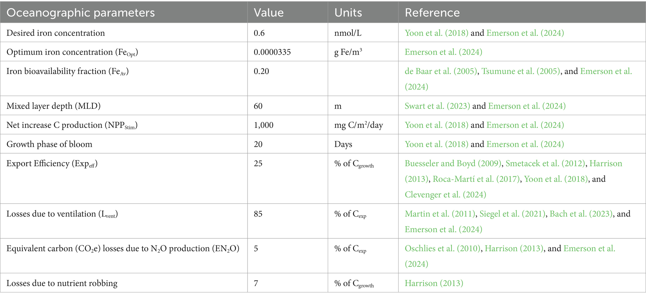
Table 1. Oceanographic model inputs.

Material flows for all pipelines were calculated for liquid flows (seawater, hydrochloric acid, and product) to achieve a velocity between 1 and 3 m/s, as recommended by standard engineering guidelines (Sinnot and Towler, 2009). The pressure drop and work required to move fluids through each pipeline were determined using the equivalent pipe diameter method, while the power requirements for each pump were calculated based on assumed efficiency and the associated pipeline work (Sinnot and Towler, 2009). The power requirements for the mixing tanks were estimated based on ranges provided for similar medium-sized, agitated baffled tanks (Sinnot and Towler, 2009). The power requirements for the solid screw conveyors (GN Solids Control, 2021) and bucket elevators (ADM Packaging Automation, 2018) were derived from industry sources based on the flow rate (t/h) and the size (m³) of the equipment required for the case study. Power for all vessel-based activities was assumed to be supplied by onboard diesel-electric generators, necessitating additional fuel beyond that needed for vessel propulsion. Future fuel mixes could potentially include renewable energy sources; however, the costs of conventional fossil fuels were considered here as a conservative scenario. The total power requirements were calculated for 24-h operation, with continuous operation for most process equipment (see Section 2.5).

2.5 Process equipment

A dedicated 1,500 deadweight tonnage (DWT) modified tanker (Figure 3) was used for all process operations, as it is large enough for long ocean voyages, ensuring sufficient capacity for all required fuel, materials, and personnel. The modified process vessels each have a maximum speed of 12 knots, a maximum cargo capacity of 800 metric tonne (t), and an engine power requirement of 1880 kW based on industry design specifications (Norden Ship Design House, 2024). The vessels were modified to include storage and mixing equipment to continuously produce a 9.94 kg/s (~0.01 m³/s) stream of acidified iron sulfate solution (pH 2), which is dispersed into the prop wash.

Figure 3

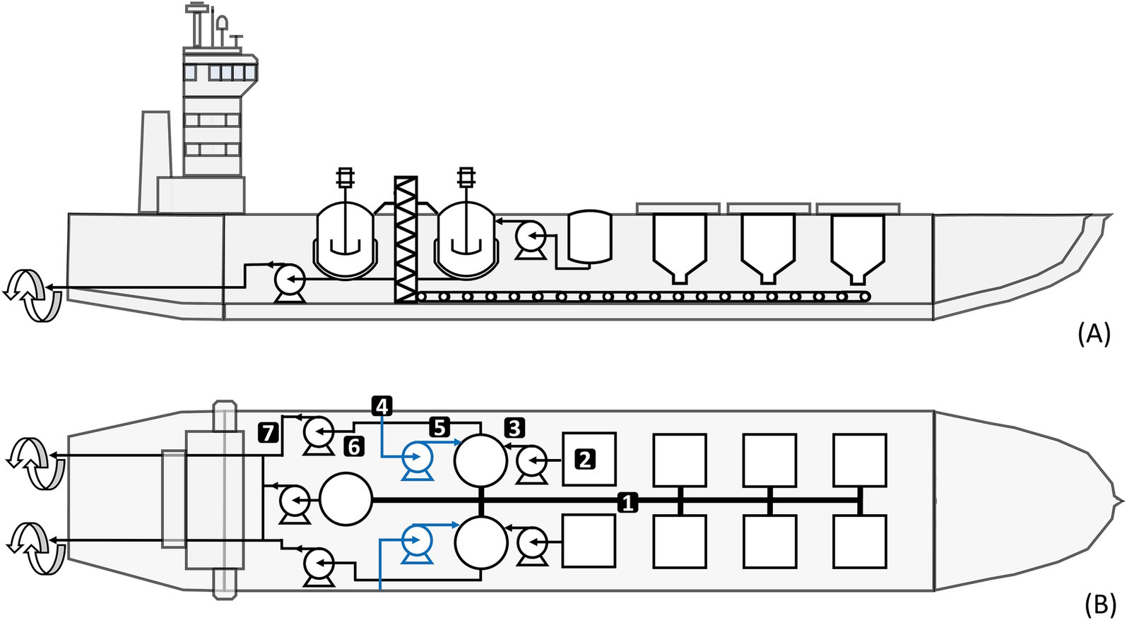
Figure 3. OIF vessel process flow diagram. (A) Vessel Side view. (B) Vessel top-down view. Streams represent (1) Iron sulfate (FeSO₄·7H₂O) mixer input, (2) HCl mixer input (pre-pump), (3) HCl mixer input (post-pump), (4) Seawater input (pre-pump), (5) Seawater input (post-pump), (6) Acidified iron sulfate solution output from mixer (pre-pump), (7) Acidified iron sulfate solution output from mixer (post-pump).

Six storage tanks were assumed for the iron sulfate and two for the 30 wt% HCl solution to evenly distribute weight and reduce safety risks from leakage or human contact. Centrifugal pumps transferred HCl (0.02 kg/s) and seawater (8.74 kg/s) into the mixing tanks. Screw conveyors and bucket elevators moved solid iron sulfate (1.18 kg/s) to the tanks. The process occurred continuously, and two mixing tanks were used in a mixing/dispersing rotation to allow for maintenance and cleaning intervals. To mitigate the impact of downtime and provide redundancy, especially since repairs may not be feasible when sailing hundreds to thousands of kilometers from port, a backup mixing tank/system was included on each vessel.

Table 2 shows the major model inputs. The minimum number of process vessels was determined to be 14, based on the maximum cargo capacity, the total mass of FeSO₄·7H₂O and HCl for a single deployment (comprising three applications), and the mass of seawater required for 1 h of operation. An overestimation of seawater storage capacity (1 h estimated vs. ~5 min actual holdup) provided weight redundancy to ensure flexibility in vessel capacity for extra fuel (allowing for longer travel distances) and iron sulfate storage (allowing for additional iron addition). The time required for spreading and transport is based on the distance traveled and the speed of the vessels. One deployment (comprising three applications) occurs annually to account for the growth of phytoplankton and the measurement of biomass export.

Table 2

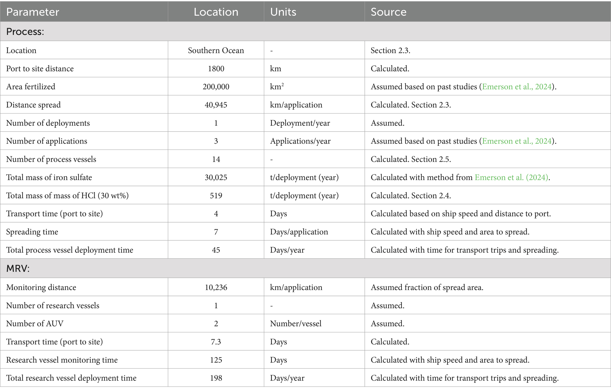
Table 2. Major model inputs/assumptions.

The average specific fuel consumption for all process vessels was estimated as 0.2 kg/kWh for medium-sized marine diesel oil (MDO)-fueled engines, utilizing literature sources (Marques et al., 2017; Tadros et al., 2019; Sofen et al., 2023) and industry insights (Sustainable Ships, 2024). Research vessels were assumed to have a fuel consumption of 0.25 kg/kWh to account for slower movement due to the deployment of AUVs and ocean sampling procedures. It was assumed that the vessels constantly operated at 85% of maximum speed and the associated engine load. MDO was chosen as the fuel for all vessels, following the increasing trend of usage in the international shipping sector compared to the more conventional heavy fuel oil (Faber et al., 2020), along with the potential for stricter emissions regulations in the future that may economically inhibit the use of heavy fuel oil.

The costs of process equipment (vessel process plant) were calculated using the cost correlation method outlined by Woods (2007). All costs were adjusted to 2023 USD ($) using a Chemical Engineering Plant Cost Index (CEPCI) value of 798, consistent with the annual value for 2023 (797.9) as reported by Anonymous (2024). Each cost element within the model is assumed to reflect 2023 USD ($). No location adjustments were considered, as it was assumed that the vessels would be retrofitted in the USA or Europe. Process vessel capital costs were determined to be $7 M per vessel by averaging the costs of five chemical tanker vessels with similar DWT from online industry sources (Nautilus Shipbrokers, 2024), assuming a conservative depreciation/inflation factor of -10% per year (Ådland et al., 2004).

Monitoring, reporting, and verification (MRV) costs related to carbon tracking (e.g., biomass generation, export to the deep ocean) and environmental/ecological tracking (e.g., ecosystem balance, nutrient concentrations) were preliminarily addressed in the model by the capital costs associated with a research vessel and AUV, as well as the operational costs of labor (science team, including ocean modeling studies), fuel (research vessel), and satellite monitoring. The inclusion of the research vessel (for point source measurement), satellites (for high-resolution mapping), and AUVs (for variable source measurements) was intended to cover a wide array of possible ocean parameters, such as chlorophyll, pH, nutrients, nitrous oxide (N₂O), oxygen (O₂), and marine species, among others (Emerson et al., 2024). It was assumed that the research vessel could deploy sediment traps and any necessary AUVs to capture subsurface biogeochemical measurements and carbon export (National Academies of Sciences Engineering and Medicine, 2022). As OIF is currently in the early stages, while the case study assumes it is at a mature stage (TRL ~ 9), the precise requirements for MRV remain uncertain. Consequently, the model does not constrain specific MRV pathways but encompasses a wide range of measurement approaches that may be required under the current assumptions. Research vessels were incorporated conservatively into the model’s baseline scenario, but they may not be necessary for MRV in more advanced future scenarios should ocean models, autonomous sampling, or other forms of carbon tracking develop further. Additionally, any broader environmental effects of OIF deployment (e.g., downstream nutrient robbing, ecosystem balance) that need to be characterized for a mature technological deployment were assumed to be addressed through long-term monitoring associated with subsequent OIF deployments. The OIF deployment location was assumed to remain constant each year. The logistics of future deployments considered the required carbon and environmental monitoring/measurement locations from prior deployments to establish an efficient deployment path for vessels and equipment. In summary, future deployments were assumed to measure oceanic parameters based on current and past deployments through a comprehensive MRV and environmental quality control process. The specified equipment requirements, logistical considerations, and assumptions regarding the scientific knowledge essential for deployment (Section 2.2) were designed to enable the quantification of carbon sequestered and its assignment to the specific OIF process (ensuring additionality), as well as the determination of environmental side effects, laterally (surface area) and vertically (depth) across oceans in accordance with the suggested mCDR monitoring system requirements (Boyd et al., 2023; Doney et al., 2025; Halloran et al., 2025). These requirements accounted for the inherent mixing and dilution effects of the ocean (Doney et al., 2025). The oceanographic research vessels (approximately 50 m in length) were projected to have an average speed of 6.5 knots and a combined engine power of 3,530 kW (see existing vessels such as Reformar, 2021). The capital cost of research vessels was estimated at $120 M, based on industry sources for similar vessels (U.S. National Science Foundation, 2018; The Maritime Executive, 2021; Hereon, 2024). Each research vessel was outfitted with two autonomous underwater vehicles (AUVs), estimated to cost $4 M each (industrial quote from Ocean Nourishment Corporation, 2024). A research vessel was included as standard to assess the impact of owning and operating all equipment for the process compared to externally chartering another vessel. The research vessel was assumed to return to port five times during the expeditions for refueling and resupplying.

2.6 Capital expenditure

The capital expenditure (CAPEX) was estimated using the methodology provided by DOE/NETL (Rubin et al., 2013; Theis, 2021; Henry et al., 2023). The costs are presented in real 2023 dollars, excluding the effects of inflation. The equipment costs were considered the bare erected cost (BEC), which includes the process equipment, supporting facilities, and direct/indirect labor costs. Engineering, procurement, and construction (EPC) contractor services were estimated at 15% of BEC (Rubin et al., 2013). The process contingency was set at 40% to reflect the limited data and operational experience of OIF as a CDR approach (Rubin et al., 2013). The project contingency was also set at 40% to conservatively demonstrate an AACE Class 4 cost estimation (Rubin et al., 2013; Theis, 2021). Owners’ costs include pre-production (startup), inventory capital, financing, and other site-specific owners’ costs. The costs of fuel and chemicals (FeSO₄·7H₂O, HCl) within the pre-production (startup) and inventory capital owners’ costs were adjusted to account for the reduced yearly operating time (~45 days) compared to year-round energy generation processes that the standard methodology is based upon (~365 days). The pre-production (startup) and inventory capital owners’ costs were calculated according to Theis (2021) and adjusted to ensure the same fractional cost for materials per year despite the reduction in operating time. Financing was set at 2.7% of the total plant cost (TPC), and other owners’ costs were set at 15% of TPC, following standard guidelines for process plants (Theis, 2021). These cost values were assumed to include ocean mapping/feasibility studies, the construction of additional port facilities (e.g., loading cranes/distribution), and legal/permitting fees associated with ocean operations. The total as-spent capital investment was determined assuming a capital distribution of 10, 60, and 30% over a 3-year period with a discount rate of 10% (Henry et al., 2023).

2.7 Bottom-up business costing

The likely route to large-scale deployment of CDR approaches may feature profit-driven businesses. As a result, it is crucial to account for the costs of business operations (total labor) as well as CDR deployment (process operations) when conducting TEA of such novel approaches. To explore whether business costs are accurately accounted for within current TEA methods, bottom-up business costing was implemented. A pseudo-CDR business structure was created based on that of operating companies and industry experience regarding the expertise required in the CDR field. The business was formed of multiple teams, each with a lead/executive who oversees operations, as shown for operating labor in Table 3 and administrative and support labor in Table 4. The number of people required for each role was combined with the salaries of the closest possible roles from the U.S. Bureau of Labor Statistics (2024) and an additional 30% labor burden (Schmitt et al., 2022) to provide an indicative operational cost of labor for the business. The total operational labor includes administrative support (including leadership) as well as operating labor (process operators, vessel crew, and MRV science personnel).

Table 3

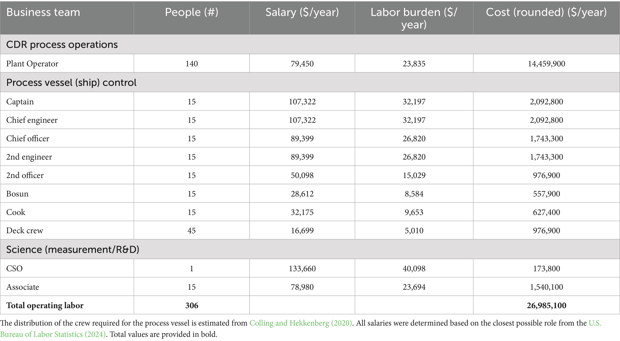
Table 3. Bottom-up business costing—operating labor.

Table 4

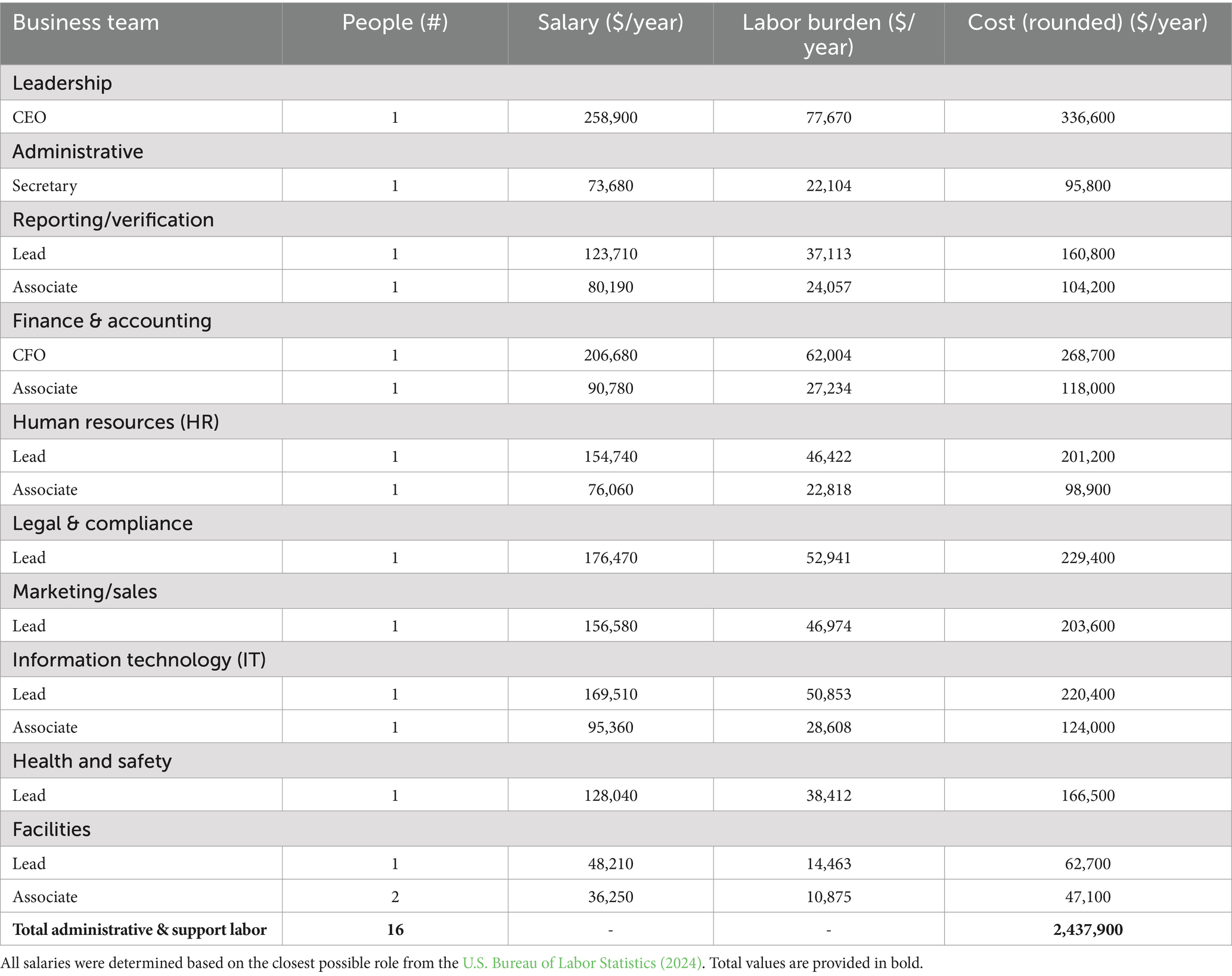
Table 4. Bottom-up business costing—administrative and support labor.

The operating labor includes the personnel responsible for running all process operations and conducting on-the-water scientific measurements and AUV operations. The estimated number of people required for process operations on each vessel is 10, based on the number of transport (pumps/conveyor) and mixing process operations for each vessel. The required crew size for each vessel was estimated conservatively, using the standards set for larger vessels (Colling and Hekkenberg, 2020). The science personnel ensured that any necessary samples were collected during MRV cruises, AUVs were deployed as needed, and research into more efficient deployment methods was pursued.

The administrative and support labor comprises all personnel essential for running a CDR business that conducts ocean iron fertilization. The standard core business teams, including leadership, administration, finance and accounting, human resources (HR), information technology (IT), and facilities, are essential for managing the company, its people, and the information stored in internal and external systems. However, several additional teams are required. A reporting and verification team ensures that all data is available to generate carbon credits, the core of a CDR business. A legal and compliance team ensures adherence to local and international laws and regulations in the ocean space. A marketing and sales team promotes the credits generated by the business and enhances the company’s reputation to drive growth. A health and safety team ensures the safety of all affected individuals, as conducting offshore process activities poses inherent risks.

2.8 Operational expenditure

The operating expenditure was estimated using the methodology provided by DOE/NETL, except for the maintenance labor and materials, which followed the IEAGHG method (Rubin et al., 2013). The nomenclature recommended by Rubin et al. (2013) was adopted to ensure that the proposed framework is comprehensive and consistent, given that the novel mCDR approach has process-specific considerations. For the fixed operating costs, the operating labor was determined through bottom-up business costing, specifically for the process operators, vessel crew, and MRV science personnel. The total maintenance cost (TMC) was set at 2.5% of the total plant cost (TPC) (Rubin et al., 2013). The maintenance labor accounts for 40% of the TMC, while maintenance materials constitute 60% of the TMC (Rubin et al., 2013). Administration and support labor was taken as 25% of the burdened operating and maintenance labor (Rubin et al., 2013). Insurance was calculated as 2% of the total plant cost (Rubin et al., 2013). Marine CDR-specific items, including vessel maintenance, AUV maintenance, and carbon credit verification, were additionally included as 1% of the process and research vessel capital costs (a conservative estimate from Konovessis, 2012), $100,000 per AUV per year (an industrial quote from Ocean Nourishment Corporation, 2024) $5,000 (Verra, 2023), respectively.

To calculate the variable operating costs, the mass of fuel (process & research (MRV) vessels) and chemicals required was multiplied by conservative prices for iron sulfate (FeSO₄·7H₂O, $350/t), hydrochloric acid (HCl, $200/t), and marine diesel oil (MDO, $1,000/t) (Harrison, 2013; Babakhani et al., 2022; Future Fuels and Technology Project, 2024; Ship & Bunker, 2024). The waste disposal and byproduct sales costs were excluded because they do not apply to the process. CO₂ transport costs were not included separately, as they were incorporated into labor and fuel costs. The operational costs of CO₂/carbon monitoring and measurement (satellite monitoring of biomass growth and storage for OIF) were included within the CO₂ storage term, similar to DOE/NETL’s guidelines for CCS (Henry et al., 2023). This was estimated as $0.2/tCO₂, which is 2.5 times an industry quote of approximately $80,000 (60,000 GBP) (Pixalytics Ltd., 2024) for activities related to a similar 1Mt scale process. The quote was increased several times to account for uncertainties between mCDR approaches and the required thoroughness of MRV. Any additional equipment or operational expenses were not quantified. The cost of offsetting all carbon dioxide emitted in the process (emissions tax) through schemes such as the EU ETS (European Commission, 2024) was not included, as the process is net negative. An additional term for variable carbon credit verification costs was needed to address the expenses associated with verifying carbon credits through external parties such as Verra. This was included in the model as a combined VCU issuance levy and methodology compensation rebate cost ($/tCO₂) for each carbon credit (1 tCO₂) generated (Verra, 2023). The cost of developing a methodology for carbon credit verification was not necessary, assuming that a methodology has been established in future deployment scenarios. The total operating cost is the sum of fixed and variable operating costs.

Several costs were included in addition to those outlined in the framework by Rubin et al. (2013) and the methodologies provided by DOE/NETL and IEAGHG to create a framework applicable to novel CDR/mCDR approaches. These costs encompass the maintenance of process and MRV (monitoring, reporting, and verification) vessels, as well as the fixed or variable verification expenses for third-party verification of data and carbon credits. Labor costs for vessel operation, monitoring by the science team, and fuel for process/research vessels and MRV equipment were included as both fixed and variable operating costs.

2.9 Cash flow/economic indicators

Cash flow analysis was based on the method outlined by Towler and Sinnott (2022), with the inclusion of interest during construction added to the CAPEX, following a distribution of 10, 60, and 30% over 3 years (Henry et al., 2023), and utilizing a discount rate of 10% as an average for the base case scenario. The levelized cost of carbon (LCOC, $/tCO₂ net-removed) was determined using the equation adapted from van der Spek et al. (2017):

$\mathit{LCOC}=\frac{{\displaystyle \sum }_{t=1}^n\frac{VO{M}_t+FO{M}_t+C\mathrm{A}PE{X}_t}{{\left(1+r\right)}^t}}{{\displaystyle \sum }_{t=1}^n\frac{NetC{O}_2\mathit{Remove}{d}_t}{{\left(1+r\right)}^t}}\text{,}$

where VOM_t is the annual variable O&M costs in year t ($/year), FOM_t is the annual fixed O&M costs in year t ($/year), CAPEX_t is the capital expenditure distributed in year t ($/year), Net CO₂ Removed_t is the net amount of CO₂ removed by the process in year t (t CO₂/year), r is the discount rate, and n is the total number of years from construction to end of project life.

2.10 Prospective (ex-ante) NOAK analysis

While the FOAK costs are also prospective in nature, the NOAK levelized cost of carbon was determined for various plant capacities using learning rate equations (IEAGHG, 2021):

$y=a{x}^{-b}$

$b=-\frac{ln\left(1-LR\right)}{ln\left(2\right)}$

where y is the CAPEX or OPEX for a specified NOAK plant capacity, a is the CAPEX or OPEX for the FOAK plant capacity, x is the ratio of current cumulative capacity to initial capacity, b is the learning rate exponent for a doubling of plant capacity, and LR is the fractional learning rate.

Estimations of the possible upper scale of ocean fertilization range from 100 Mt. to 1,000 Mt., considering the environmental and legal constraints of large-scale deployment (Scott-Buechler and Greene, 2019; National Academies of Sciences Engineering and Medicine, 2022; Bach et al., 2023). The NOAK scale was set conservatively at 10 Mt., approximately 10 times the capacity of the FOAK base case scenario, to ensure that possible environmental implications were limited and the area required for fertilization (~2,000,000 km², ~0.6% of the world’s ocean area) was within the constraints of available high nitrate low chlorophyll (HNLC) regions (~30–40% of the ocean) (Emerson, 2019). The locations for OIF were assumed to vary as the business scales since nutrient limitations from additional growth will reduce the efficiencies of OIF when conducted in an ever-increasing area (Ianson et al., 2012).

A conservative 5% learning rate for the process as a whole was applied to the total plant cost (TPC) based on the assumption that the learning rate was similar to other emerging industries (Thomassen et al., 2020; IEAGHG, 2021). Since the fixed OPEX is dependent on this variable, except for the majority of labor, vessel maintenance, and carbon credit verification costs, the fixed OPEX changed accordingly. While minor reductions in labor costs due to improved learning may be possible, this was assumed to be negligible, as costs would likely not continue to decrease with each doubling of carbon removal (plant) capacity. Vessel maintenance is already an established industry, and carbon credit verification costs are set by third parties. Therefore, these fixed costs were also assumed to be unchanging. A separate conservative learning rate of 5% for the variable OPEX was applied to account for potential changes in variable operating costs (IEAGHG, 2021). Variations in the learning rates from the base case scenario were included in an uncertainty analysis (Section 3.3).

3 Results and discussion

3.1 Scenarios – base case

Table 5 presents a comparison of the FOAK and NOAK OIF deployment costs for the base case scenario. The NOAK scale for the base case is 10 Mt., illustrating a feasible size for a realistic carbon removal company operating in this field (Section 2.10). The NOAK sensitivity analysis (Section 3.3) examines a broad range of scales (CO₂ removal capacity) and the impact this has on the NOAK LCOC. The deployment costs in the Southern Ocean are approximately $205/t CO₂ for the FOAK process (~1 Mt) and about $180/t CO₂ for the NOAK process (~10 Mt). Although these costs exceed the industry goal of $100/t CO₂ (National Academies of Sciences Engineering and Medicine, 2022)_, the base case costs for FOAK and NOAK scenarios reflect the cost potential of OIF. However, the parameters and costs that comprise these values are based on key assumptions, which can adversely (increase costs from the base case) or favorably (reduce costs from the base case) affect the outcome.

Table 5

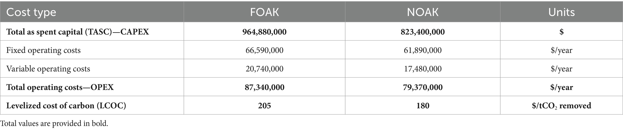
Table 5. FOAK vs. NOAK cost comparison: values represent a single deployment operation for the FOAK scale (~1 Mt. CO₂ removal) and per several deployment operations for the NOAK scale (10 Mt. CO₂ removal).

The assumptions for administrative and support labor within standard DOE/NETL cost estimates (25% of O&M labor) (Rubin et al., 2013) indicate higher labor costs (FOAK, $8,316,800 per year) compared to small- to medium-scale businesses using the proposed bottom-up business costing method (Section 2.7, FOAK, $2,437,900 per year). For the cost analysis of small- to medium-scale businesses, such as those operating in the CDR space, this result suggests that the cost of administrative and support labor should be adjusted based on the outcomes of a bottom up business costing. Furthermore, total labor costs account for approximately 48% of the total operating costs of the process, utilizing bottom-up business costing for operating labor and standard methodologies for administrative and support and maintenance labor. Operating labor accounts for 31% of total operating costs, highlighting the importance of conducting bottom-up business cost analyses to determine labor costs when dealing with similar novel CDR processes.

Furthermore, the cost impact of operating a dedicated research vessel for monitoring carbon removal through biomass generation and export is included in the model’s base case scenario. As discussed further in the sensitivity analysis, the capital expenditure for such a cutting-edge vessel (~$120 M base case) with 2 AUVs ($8,000,000) has a substantial impact on the final LCOC. Investigating the use of a purchased vessel and AUV versus one chartered at a rate of $50,000 per day, assumed to include fuel (Emerson et al., 2024), results in a reduction of the FOAK LCOC from the base case value of $205 per tCO₂ to $146 per tCO₂. In addition to the challenges of securing financing for a research vessel, these results indicate that it is much more economical to charter a research vessel for OIF deployment purposes compared to purchasing one outright, except potentially in cases of large-scale OIF or other combinations of ocean CDR deployment. In such situations, there may not be enough capacity to charter research vessels for a sufficient duration to accurately constrain CO₂ removal. For this reason, the capital expenditure for a research vessel, along with the costs of AUVs, fuel, crew, and maintenance, is included as standard in the model.

Additionally, the impact of process emissions (Table 6) from material production, transport, spreading, and MRV stages is much lower overall (10,208 tCe/year) than the offsets due to N₂O production (139,500 tCe/year), carbon losses from nutrient robbing (840,000 tCe/year), carbon losses due to CO₂ ventilation (2,371,500 tCe/year), and export efficiency (8,370,000 tCe/year). This indicates that oceanographic parameters play a key role in the final net carbon removed by the OIF process (C_net) and, consequently, in the final levelized cost of carbon.

Table 6

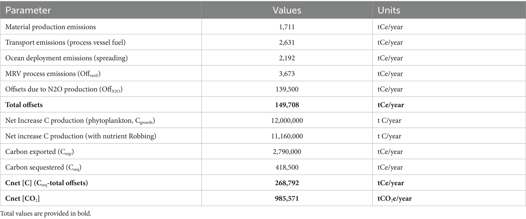
Table 6. Carbon balance.

3.2 Uncertainty analysis – FOAK

The parameters considered in the model included the major stages of OIF deployment: material production, material transport to the ocean, material deployment, and monitoring, reporting, and verification. However, the uncertainty in the chosen parameters necessitates conducting an uncertainty analysis to determine whether variation in these parameters significantly impacts the LCOC. A local sensitivity analysis was used to achieve this goal for the FOAK and NOAK costs at the selected location.

A local sensitivity analysis was conducted on 26 of the main input parameters to determine the impact of a range of possible variations in each parameter on the FOAK LCOC. Each parameter was varied individually. Not all parameters were varied by the same percentage base case +/− as physical (e.g., number of people ≠ ≤ 1), scientific (e.g., values < experimental), and economic (e.g., iron sulfate price < industry maximum) constraints were set for each parameter individually (see Supplementary Materials). Additionally, the same percentage changes were not essential for comparison, as some parameters may vary more than others (e.g., price vs. number of MRV (research) vessels). A total of 10 linearly spaced points were used as standard unless the parameters required fewer or more to demonstrate a trend.

The engineering costs that have a significant impact on LCOC include the process vessel cost (Δ = overall variance = ~$55/tCO₂), research vessel cost (Δ ~ $59/tCO₂), the number of process vessels (Δ ~ $85/tCO₂), and the number of MRV (research) vessels (Δ ~ $132/tCO₂) (Figure 4). The substantial impact on the levelized cost from the quantity and cost of research vessels arises from the extremely high capital expenditure required for each vessel. The process vessel cost also has a notable impact on the levelized cost, especially when compared to the MRV AUV cost (Δ ~ $2/tCO₂; see Supplementary Material), due to the high capital expenditure associated with the total number of vessels. This indicates that capital outlay must be significant (~$120–160 M) to impact the levelized cost of carbon meaningfully. Other studies have described the high variability of MRV costs from both research and industry perspectives (5–300% of total costs) (Emerson et al., 2024; Mercer et al., 2024). Furthermore, the results of this study suggest that the major capital cost items of MRV, such as research vessels and AUV equipment, have a more substantial effect on the levelized cost of OIF. In contrast, operational costs, including the fuel consumption of the research vessels, satellite monitoring, or scientific personnel, have a minor overall cost impact. Consequently, to achieve accurate carbon tracking and environmental monitoring through a combined MRV process, minor variations in operational costs of consumables and personnel are unlikely to affect the economic feasibility of the process.

Figure 4

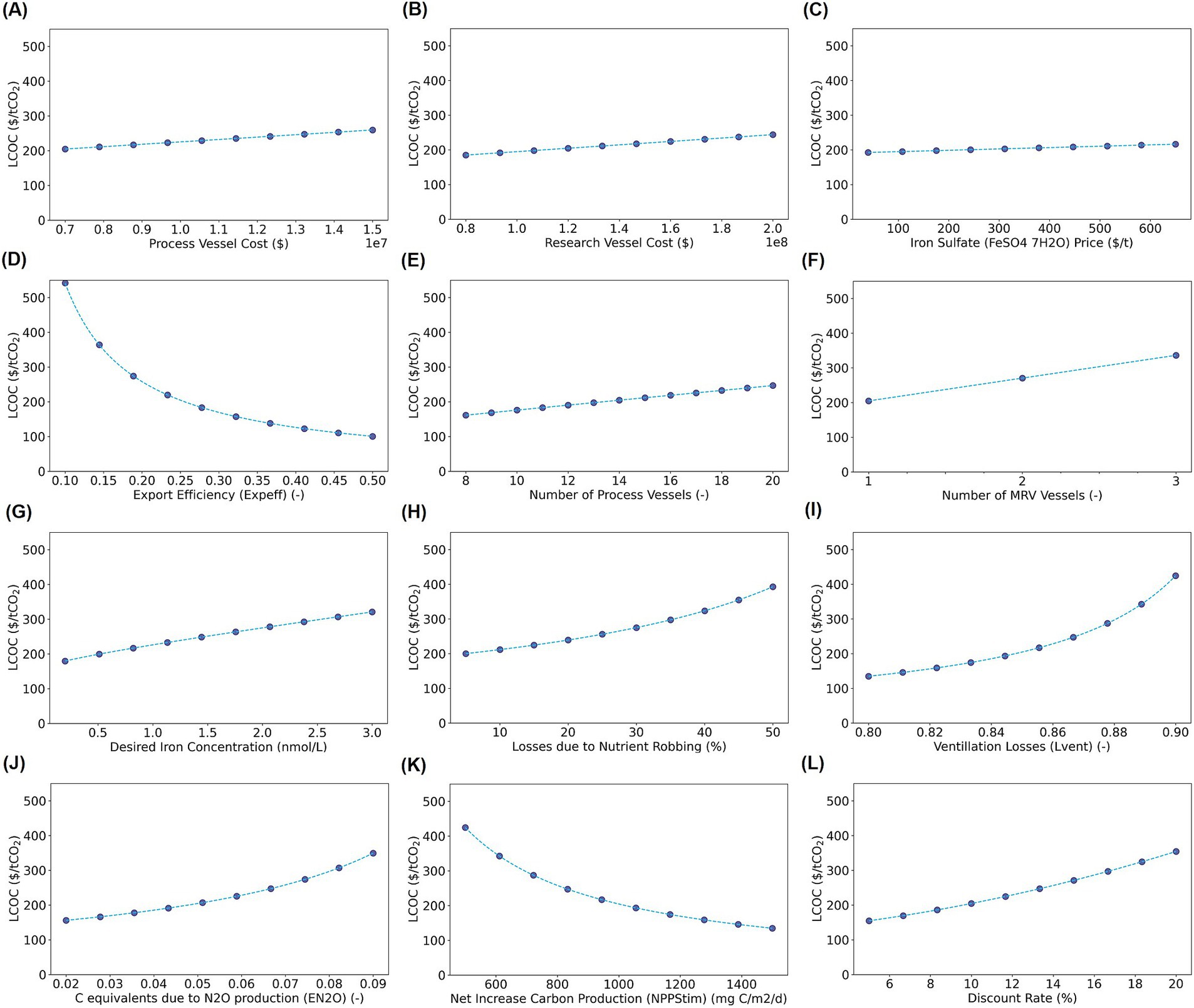
Figure 4. Sensitivity analysis of major parameters. Results of the FOAK local sensitivity analysis illustrate the effects of (A) process vessel cost, (B) research vessel cost, (C) iron sulfate price, (D) export efficiency, (E) number of process vessels, (F) number of MRV (research) vessels, (G) desired iron concentration, (H) losses due to nutrient robbing, (I) losses from ventilation of CO₂, (J) equivalent carbon (CO₂e) losses due to N₂O production, (K) net increase in carbon production, and (L) discount rate on the FOAK levelized cost of carbon ($/tCO₂ removed).

The results also suggest that the distance between locations in the geographic northern and southern regions of the world is not a significant factor for cost, as the distance from the port to OIF deployment sites has a minimal effect on the LCOC (Δ ~ $11/tCO₂ with Δ ~ 3,500 km; see Supplementary Materials). Additionally, the interconnectivity of global shipping routes and ports limits the transport distance and, thereby, this cost variance. The price of iron sulfate has a minor influence on the LCOC (Δ ~ $24/tCO₂) across a wide range of values ($40–650/t FeSO₄·7H₂O). When operating at scale, with other parameters characterized and efficiencies realized, minimizing costs due to material prices may be essential for profitability and, unlike oceanographic parameters, can be negotiated. However, overall, the oceanographic parameters exert the most notable influence on the FOAK LCOC. Losses due to nutrient robbing (Δ ~ $193/tCO₂), equivalent carbon (CO₂e) losses due to N₂O production (Δ ~ $193/tCO₂), desired iron concentration (Δ ~ $141/tCO₂), losses due to ventilation of CO₂ (Δ ~ $290/tCO₂), net increase in carbon production (Δ ~ $290/tCO₂), and, most significantly, export efficiency (Δ ~ $441/tCO₂) have the potential to drastically vary the final cost of an OIF deployment. The discount rate also has a significant effect on the LCOC (Δ ~ $200/tCO₂), highlighting the need to constrain certain economic parameters as well as the oceanographic parameters to provide accurate cost estimations.

Plotting the sensitivity results as a tornado diagram (Figure 5) further demonstrates the cost variance due to oceanographic parameters but also highlights that some parameters have a higher input sensitivity than others. Notably, equivalent changes in the values for losses due to the ventilation of CO₂, net increase in carbon production (NPP Stim.), and export efficiency change the final LCOC significantly more than all other parameters. As these are oceanographic parameters that cannot be fully constrained except with further ocean experiments, there will always be a wide range for OIF cost estimates until certainty for large-scale OIF can be established. However, if future studies could better characterize the probabilities that certain ranges of input values exist for specific locations or scenarios, the more sensitive input parameters, along with the LCOC, could be better constrained to provide probabilistic costs.

Figure 5

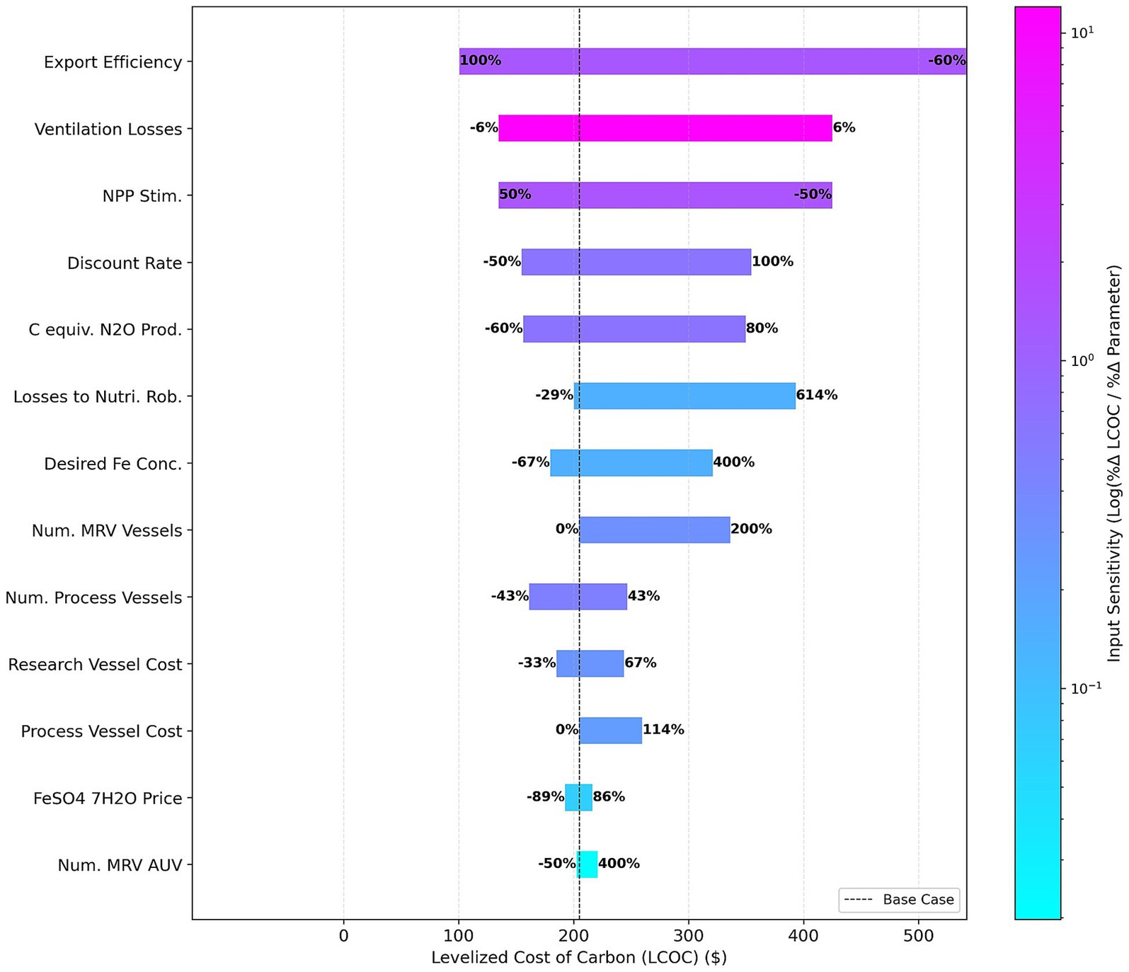
Figure 5. Tornado diagram showing a summary of input parameter variance on the FOAK levelized cost of carbon ($/tCO₂ removed). The values (%) next to each bar indicate the percentage change of an input parameter from the base case (dashed line). The color bar represents cost sensitivity to input parameters within the model, calculated as the average overall % change in LCOC from the base case cost divided by the average overall % change in input parameters from base case values. Small input changes resulting in large cost changes incur higher sensitivity values (purple/pink), while large input changes that result in small to medium cost changes incur lower sensitivity values (blue).

Additionally, there are indications that the iron bioavailability fraction has a major impact on the LCOC. However, this parameter was not varied because it affected the physical constraints of the process (e.g., number of process vessels (ships), capacity of process vessels, process equipment design, and time of deployment), which required manual corrections within the model due to the interconnectivity of various design parameters. A lower iron bioavailability fraction necessitated a larger processing capacity for the product solution (acidified iron sulfate), resulting in the need for more process vessels (ships) and larger equipment. The number of process vessels could be reduced by increasing the size of the ships or ensuring the availability of refueling/resupplying ships, but these options fall outside the scope of this study. All other varied input parameters have a comparatively low impact on the LCOC (Δ < $20/tCO₂) according to the specified minimum and maximum ranges (see Supplementary Material).

Other studies have found significant variations in cost estimates for OIF, ranging from $30 to $300 per tonne of CO₂ removed (Babakhani et al., 2022), approximately $6 to $1,280 per tonne of CO₂ removed (Emerson et al., 2024), and less than $100 to over $1,000 per tonne of CO₂ removed (Bach et al., 2023). These findings indicate inherent uncertainty in OIF cost estimations. Specifying the best- and worst-case values for MRV processes, losses due to nutrient robbing, equivalent carbon losses (CO₂e) due to N₂O production, ventilation losses of CO₂ to the atmosphere, net increase in primary production (phytoplankton growth), and export efficiency yields a cost range of $25 per tonne CO₂ to $53,000 per tonne CO₂ (FOAK). The best scenario for MRV processes assumes that no research vessels are required, with all MRV conducted via AUV, satellite imagery, and modeling of the ocean system, using the same number of employees for the science team. While the feasibility of this scenario remains uncertain until MRV requirements and oceanographic science advance, it presents an optimistic view. Conversely, the worst-case scenario for MRV processes involves the use of a 1 research vessel, as intensive sampling immediately after deployment would be essential. The range for losses due to nutrient robbing (5 to 25% of NPP) (Aumont and Bopp, 2006; Harrison, 2013), equivalent carbon losses from N₂O production (2 to 7.5% of C_exp) (Oschlies et al., 2010; Harrison, 2013; Emerson et al., 2024), ventilation losses of CO₂ (80 to 90%) (Martin et al., 2011; Siegel et al., 2021; Bach et al., 2023; Emerson et al., 2024), and the net increase in primary production (1,500 to 500 mgC/m²/d) (Yoon et al., 2018; Emerson et al., 2024) are based on several studies, providing a potential range of scenarios. It is important to note that the ventilation losses term was capped at 7.5% since higher values resulted in no net carbon removal. The best-case scenario for export efficiency was estimated at 50%, based on shallow (~60–150 m) export values from previous OIF experiments and natural studies (Buesseler and Boyd, 2009; Smetacek et al., 2012; Harrison, 2013; Yoon et al., 2018). The worst-case export efficiency was estimated at 10%, reflecting the lower ends of these ranges (Bertram, 2011; Sanders et al., 2014; Roca-Martí et al., 2017; Clevenger et al., 2024). The maximum LCOC for the best-to-worst-case range decreases to approximately $4,400 per tonne of CO₂ if the export is set to 20% (closer to the middle of the range of export values), as the primary increase in cost stems from reduced net CO₂ removal within the process. Nonetheless, the worst-case scenario illustrates possible oceanic conditions under which OIF could become economically unfeasible and should thus be avoided. The significant change in costs for OIF deployment due to small variations in specific oceanographic parameters emphasizes the need to constrain these factors. Specific ocean locations and deployment times may provide certainty regarding oceanic parameters, leading to constrained cost estimates. This could be achieved through future long-term ocean experiments.

3.3 Uncertainty analysis – NOAK

A local sensitivity analysis was also conducted on several prospective parameters to determine the impact of variance on the NOAK LCOC (Figure 6). The learning rates for the CAPEX and variable OPEX were varied between 1 and 15%, aligning with the estimated range for other emerging industries and technologies (Thomassen et al., 2020; IEAGHG, 2021). The CAPEX learning rate (Δ ~ $53/tCO₂) had a reasonable impact on the LCOC compared to the variable OPEX learning rate (Δ ~ $8/tCO₂), likely due to the substantially higher capital costs compared to operational costs (Table 5). However, both learning rate parameters had a comparatively low impact on the LCOC despite the degree of learning applied. While there is not enough data to be conclusive, these results suggest that learning rates do not significantly affect the overall costs of deployment compared to the oceanographic parameters for cost estimates with large input variations. Specifying the best- and worst-case values for MRV processes, losses due to nutrient robbing, equivalent carbon (CO₂e) losses due to N₂O production, ventilation losses of CO₂ to the atmosphere, net increase in primary production (phytoplankton growth), and export efficiency (similar to Section 3.2), the NOAK cost range for OIF was generated (Figure 7). The large best-worst-case cost difference and rectangular shape of the OIF deployment cost range diagram further demonstrate significant uncertainty due to oceanographic parameters.

Figure 6

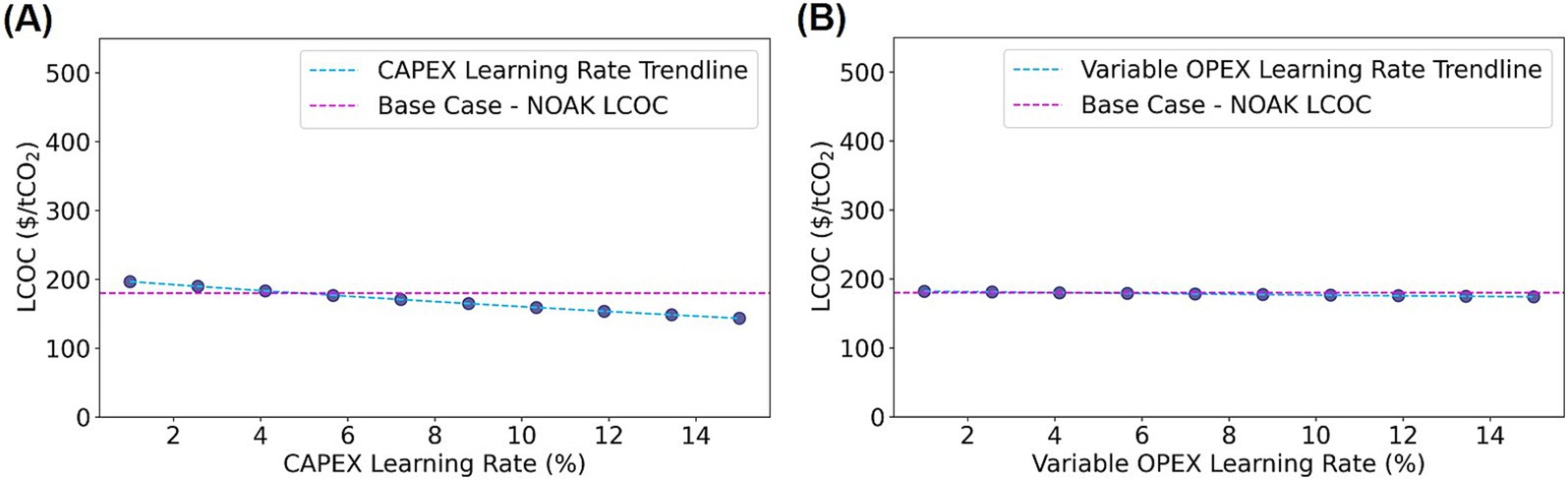
Figure 6. Sensitivity analysis of prospective factors. Results from the NOAK local sensitivity analysis demonstrate the impact of (A) the CAPEX learning rate and (B) the variable OPEX learning rate on the NOAK levelized cost of carbon ($/tCO₂ removed).

Figure 7

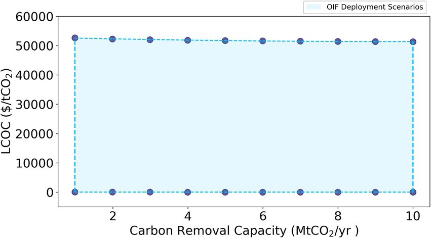
Figure 7. OIF deployment cost range. The diagram illustrates the possible range of costs for OIF deployment (y-axis) across various carbon removal capacities (x-axis). Carbon removal capacity refers to the scale of the OIF deployment scenario in terms of the carbon removed and stored in the deep ocean. Model input parameters that significantly influenced the levelized cost of carbon (see section 3.2) were varied between best-case and worst-case values. The lower horizontal trendline indicates the cost of OIF versus carbon removal capacity for the best-case input values. The upper trendline represents the cost of OIF versus carbon removal capacity for the worst-case input values. The shaded area between these trendlines depicts the potential cost of OIF for all other scenarios under the same model assumptions. Parameters varied between best-case and worst-case values (see sections 3.2, 3.3) include MRV processes, nutrient robbing losses, equivalent carbon (CO₂e) losses due to N₂O production, ventilation losses of CO₂ to the atmosphere, net increase in primary production (phytoplankton growth), export efficiency, and learning rate.

The best-case scenario assumed a learning rate of 15%, where significant process efficiencies were achieved through learning due to unforeseen scale-up requirements. The worst-case scenario assumed a learning rate of 1%, where only minimal process efficiencies were gained through learning. Both values reflect potential learnings when deploying a carbon dioxide removal technology, which is presumed to have a robust scientific foundation and is at a commercial deployment stage (TRL > =9) (Section 2.2). The difference in LCOC between the best- and worst-case scenarios (low and high horizontal trendlines) was found to decrease from the FOAK (~1 Mt) to the NOAK (~10 Mt) scales, indicating increased certainty due to learning. Additionally, the reduction in the levelized cost resulting from learning (decrease of each horizontal trendline) was found to be less economically significant (per dollar) for the best-case scenario (low horizontal trendline, LR = 15%, Δ ~ $8/tCO₂) compared to the worst-case scenario (high horizontal trendline, LR = 1%, Δ ~ $1,400/tCO₂), despite a larger percentage cost reduction in the best case (~30%) versus the worst case (~3%). The best-case costs are extremely low (~$18/tCO₂–$25/tCO₂) compared to the worst-case costs (~$51,000/tCO₂–$53,000/tCO₂) due to uncertainties in input parameters (Section 3.2). Therefore, the best-case costs remained low while the worst-case costs remained high, indicating that applying learning rates alone cannot sufficiently reduce cost ranges given significant input uncertainties. Nonetheless, the impact of learning rates within prospective cost estimation is crucial and must be considered in future models, as changes in underlying assumptions or input data could affect this outcome.

4 Conclusion

The framework provided was used to determine the prospective levelized cost of carbon for various OIF scenarios as approximately $200 per tonne of CO₂ for first-of-a-kind (FOAK) processes and approximately $180 per tonne of CO₂ for nth-of-a-kind (NOAK) processes, utilizing learning rates applied to capital and variable operating expenditures. A bottom-up business cost assessment of labor costs indicated that standard cost methodology guidelines tend to overestimate the administrative and support labor for small- to medium-scale CDR businesses. Since total labor costs account for nearly 50% of the overall operating costs of the process, it is essential that they are accurately constrained in TEA models through bottom-up business costing.

The results of a sensitivity analysis on the major model inputs indicate that oceanographic parameters, such as export efficiency, have a much larger impact on the final levelized cost of carbon compared to engineering costs, such as the prices of equipment or materials. This significant impact of oceanographic parameters on OIF cost models was also noted by Emerson et al. (2024). Additionally, this study revealed that large capital expenditures, estimated at ~$120–160 M from engineering costs such as research vessel costs, significantly influence the levelized cost. Varying the values for MRV processes, losses due to nutrient robbing, equivalent carbon (CO₂e) losses from N₂O production, ventilation losses of CO₂ to the atmosphere, net increase in primary production (phytoplankton growth), and export efficiency between best- and worst-case scenarios resulted in an excessive cost range of $25/tCO₂ to $53,000/tCO₂. The results of an nth-of-a-kind sensitivity analysis on the learning rates within the model indicated that these learning rates have a comparatively less significant impact on the overall costs of deployment and, subsequently, on future cost reductions when large uncertainties in parameter inputs are present.

Overall, the results suggest that OIF is feasible under some conditions and not feasible under others. Therefore, oceanographic parameters should be characterized more thoroughly through additional research and development before cost ranges can be accurately reduced for OIF. Methods of OIF deployment, including monitoring, reporting, and verification (MRV) processes, should also be investigated to minimize capital costs, such as those related to dedicated research vessels. Additionally, since learning rates play a crucial role in predicting future cost reductions, future studies should aim to narrow the applicable ranges for application to the CAPEX and variable OPEX within TEA models. The proposed framework, which includes a bottom-up business cost analysis, should be applied to other CDR methods to provide consistent and comprehensive comparisons of CDR approaches for companies and decision-makers. This would facilitate informed funding in the CDR sector and address essential research gaps in the pursuit of combating climate change through terrestrial and ocean-based carbon dioxide removal strategies.

Data availability statement

The original contributions presented in the study are included in the article/Supplementary material, further inquiries can be directed to the corresponding author.

Author contributions

CW: Conceptualization, Data curation, Formal analysis, Investigation, Methodology, Project administration, Software, Validation, Visualization, Writing – original draft, Writing – review & editing. RP: Conceptualization, Data curation, Methodology, Software, Validation, Writing – review & editing. SF: Conceptualization, Data curation, Formal analysis, Methodology, Project administration, Supervision, Writing – review & editing. PR: Conceptualization, Data curation, Formal analysis, Methodology, Project administration, Supervision, Writing – review & editing.

Funding

The author(s) declare that financial support was received for the research and/or publication of this article. This project has received funding from the European Union's Horizon Europe research and innovation programme under grant agreement no. 101081362.

Acknowledgments

The authors acknowledge valuable discussions with Dr. Christopher Pearce (National Oceanography Centre), Jill Storey (World Ocean Council), Dr. Nils Thonemann, Dr. Patrik Henriksson, and Mona Delval (University of Leiden), as well as Dr. Mijndert Van der Spek, Dr. Dan Su, and Dr. Isara Muangthai (Heriot-Watt University) during the production of this work. Additionally, the authors also acknowledge the advice and support received from project partners involved in the SEAO2-CDR project, of which this work is a key component.

Conflict of interest

The authors declare that the research was conducted in the absence of any commercial or financial relationships that could be construed as a potential conflict of interest.

The author(s) declared that they were an editorial board member of Frontiers, at the time of submission. This had no impact on the peer review process and the final decision.

Generative AI statement

The author(s) declare that no Gen AI was used in the creation of this manuscript.

Publisher’s note

All claims expressed in this article are solely those of the authors and do not necessarily represent those of their affiliated organizations, or those of the publisher, the editors and the reviewers. Any product that may be evaluated in this article, or claim that may be made by its manufacturer, is not guaranteed or endorsed by the publisher.

Supplementary material

The Supplementary material for this article can be found online at: https://www.frontiersin.org/articles/10.3389/fclim.2025.1509367/full#supplementary-material

References

Ådland, R., Jia, H., and Koekebakker, S. (2004). The pricing of forward ship value agreements and the unbiasedness of implied forward prices in the second-hand market for ships. Marit. Econ. Log. 6, 109–121. doi: 10.1057/palgrave.mel.9100098

Crossref Full Text | Google Scholar

ADM Packaging Automation (2018). ADM Bucket Elevator. Available online at: https://admpa.com.au/wp-content/uploads/2018/08/ADM-Bucket-Elevators-REV01.pdf (Accessed October 2, 2024).

Google Scholar

Allen, M. R., Dube, O. P., Solecki, W., Aragón-Durand, F., Cramer, W., Humphreys, S., et al. (2018). “Framing and context. In: global warming of 1.5°C. An IPCC special report on the impacts of global warming of 1.5°C above pre industrial levels and related global greenhouse gas emission pathways, in the context of strengthening the global response to the threat of climate change, sustainable development, and efforts to eradicate poverty” in Global warming of 1.5°C. eds. V. Masson-Delmotte, P. Zhai, H.-O. Pörtner, D. Roberts, J. Skea, and P. R. Shukla, et al. (Cambridge, UK and New York, NY, USA: Cambridge University Press), 49–92.

Google Scholar

Anonymous (2024). Economic Indicators. Chem. Eng. 131,:52. Available online at: https://www.proquest.com/trade-journals/economic-indicators/docview/3093913361/se-2?accountid=16064 (Accessed April 21, 2025).

Google Scholar

Arvidsson, R., Svanström, M., Sandén, B. A., Thonemann, N., Steubing, B., and Cucurachi, S. (2024). Terminology for future-oriented life cycle assessment: review and recommendations. Int. J. Life Cycle Assess. 29, 607–613. doi: 10.1007/s11367-023-02265-8

Crossref Full Text | Google Scholar

Aumont, O., and Bopp, L. (2006). Globalizing results from ocean in situ iron fertilization studies. Global Biogeochem. Cycles 20, 1–15. doi: 10.1029/2005GB002591

Crossref Full Text | Google Scholar

Babakhani, P., Phenrat, T., Baalousha, M., Soratana, K., Peacock, C. L., Twining, B. S., et al. (2022). Potential use of engineered nanoparticles in ocean fertilization for large-scale atmospheric carbon dioxide removal. Nat. Nanotechnol. 17, 1342–1351. doi: 10.1038/s41565-022-01226-w

Crossref Full Text | Google Scholar

Bach, L. T., Tamsitt, V., Baldry, K., McGee, J., Laurenceau-Cornec, E. C., Strzepek, R. F., et al. (2023). Identifying the Most (cost-)efficient regions for CO2 removal with Iron fertilization in the Southern Ocean. Global Biogeochem. Cycles 37:e2023GB007754. doi: 10.1029/2023GB007754

Crossref Full Text | Google Scholar

Bertram, C. (2011). “The potential of ocean Iron fertilization as an option for mitigating climate change” in Emissions trading: Institutional design, decision making and corporate strategies. eds. R. Antes, B. Hansjürgens, P. Letmathe, and S. Pickl (Berlin, Heidelberg: Springer Berlin Heidelberg), 195–207.

Google Scholar

Bindoff, N. L., Cheung, W. W. L., Kairo, J. G., Arístegui, J., Guinder, V. A., Hallberg, R., et al. (2022). “Changing ocean, marine ecosystems, and dependent communities. In: IPCC special report on the ocean and cryosphere in a changing climate” in The ocean and cryosphere in a changing climate: Special report of the intergovernmental panel on climate change. eds. H.-O. Pörtner, D. C. Roberts, V. Masson-Delmotte, P. Zhai, M. Tignor, and E. Poloczanska, et al. (Cambridge, UK and New York, NY, USA: Cambridge University Press), 447–587.

Google Scholar

Boettcher, M., Chai, F., Conathan, M., Cooley, S., Keller, D., Klinsky, S., et al. (2023). A Code of Conduct for Marine Carbon Dioxide Removal Research. The Aspen Institute.

Google Scholar

Boettcher, M., Chai, F., Cullen, J. J., and Lampitt, R. (2019). GESAMP working group 41: high level review of a wide range of proposed marine geoengineering techniques. International Maritime Organization.

Google Scholar

Boyd, P. W. (2008). Implications of large-scale iron fertilization of the oceans. Mar. Ecol. Prog. Ser. 364, 213–218. Available online at: http://www.jstor.org/stable/24872814 (Accessed January 11, 2024).

Google Scholar

Boyd, P. W., Claustre, H., Legendre, L., Gattuso, J.-P., and Le Traon, P.-Y. (2023). Operational monitoring of Open-Ocean carbon dioxide removal deployments: detection, attribution, and determination of side effects. In Frontiers in ocean observing: emerging Technologies for Understanding and Managing a changing ocean. Oceanography 36, 2–10. doi: 10.5670/oceanog.2023.s1.2

Crossref Full Text | Google Scholar

Boyd, P. W., Jickells, T., Law, C. S., Blain, S., Boyle, E. A., Buesseler, K. O., et al. (2007). Mesoscale Iron enrichment experiments 1993-2005: synthesis and future directions. Science 1979, 612–617. doi: 10.1126/science.1131669

Crossref Full Text | Google Scholar

Buesseler, K. O., Bianchi, D., Chai, F., Cullen, J. T., Estapa, M., Hawco, N., et al. (2024). Next steps for assessing ocean iron fertilization for marine carbon dioxide removal. Front. Clim. 6, 1–15. doi: 10.3389/fclim.2024.1430957

Crossref Full Text | Google Scholar

Buesseler, K. O., and Boyd, P. W. (2009). Shedding light on processes that control particle export and flux attenuation in the twilight zone of the open ocean. Limnol. Oceanogr. 54, 1210–1232. doi: 10.4319/lo.2009.54.4.1210

Crossref Full Text | Google Scholar

Buesseler, K., Chai, F., Karl, D., Ramakrishna, K., Satterfield, T., Siegel, D., et al. (2022). Ocean Iron Fertilization: Assessing its potential as a climate solution. Available online at: http://oceaniron.org (Accessed April 21, 2025).

Google Scholar

Clevenger, S. J., Benitez-Nelson, C. R., Roca-Martí, M., Bam, W., Estapa, M., Kenyon, J. A., et al. (2024). Carbon and silica fluxes during a declining North Atlantic spring bloom as part of the EXPORTS program. Mar. Chem. 258:104346. doi: 10.1016/j.marchem.2023.104346

Crossref Full Text | Google Scholar

Colling, A., and Hekkenberg, R. (2020). Waterborne platooning in the short sea shipping sector. Transp. Res. Part C Emerg. Technol. 120, 1–15. doi: 10.1016/j.trc.2020.102778

Crossref Full Text | Google Scholar

de Baar, H. J. W., Boyd, P. W., Coale, K. H., Landry, M. R., Tsuda, A., Assmy, P., et al. (2005). Synthesis of iron fertilization experiments: from the Iron age in the age of enlightenment. J. Geophys. Res. Oceans 110, 1–24. doi: 10.1029/2004JC002601

Crossref Full Text | Google Scholar

Doney, S. C., Wolfe, W. H., McKee, D. C., and Fuhrman, J. G. (2025). The science, engineering, and validation of marine carbon dioxide removal and storage. Annu. Rev. Mar. Sci. 17, 55–81. doi: 10.1146/annurev-marine-040523-014702

Crossref Full Text | Google Scholar

Emerson, D. (2019). Biogenic Iron dust: a novel approach to ocean Iron fertilization as a means of large scale removal of carbon dioxide from the atmosphere. Front. Mar. Sci. 6, 1–8. doi: 10.3389/fmars.2019.00022

Crossref Full Text | Google Scholar

Emerson, D., Sofen, L. E., Michaud, A. B., Archer, S. D., and Twining, B. S. (2024). A cost model for ocean Iron fertilization as a means of carbon dioxide removal that compares ship- and aerial-based delivery, and estimates verification costs. Earths. Future 12:e2023EF003732. doi: 10.1029/2023EF003732

Crossref Full Text | Google Scholar

Encyclopædia Britannica (2024). Thermohaline circulation. Available online at: https://www.britannica.com/science/thermohaline-circulation (Accessed September 17, 2024).

Google Scholar

European Commission (2024). Guidance Document: The EU ETS and MRV Maritime General guidance for shipping companies. Available online at: https://climate.ec.europa.eu/document/download/31875b4f-39b9-4cde-a4e2-fbb8f65ee703_en?filename=policy_transport_shipping_gd1_maritime_en.pdf (Accessed September 18, 2024).

Google Scholar

Faber, J., Hanayama, S., Zhang, S., Pereda, P., Comer, B., Hauerhof, E., et al. (2020). Fourth IMO GHG study. International Maritime Organization.

Google Scholar

Future Fuels and Technology Project (2024). Prices of Alternative Fuels. Available online at: https://futurefuels.imo.org/home/latest-information/fuel-prices/ (Accessed September 18, 2024).

Google Scholar

GN Solids Control (2021). Screw Conveyor. Available online at: https://www.gnsolidscontrol.com/screw-conveyor (Accessed October 2, 2024).

Google Scholar

Gnanadesikan, A., Sarmiento, J. L., and Slater, R. D. (2003). Effects of patchy ocean fertilization on atmospheric carbon dioxide and biological production. Global Biogeochem. Cycles 17, 1–17. doi: 10.1029/2002GB001940

Crossref Full Text | Google Scholar

Güssow, K., Proelss, A., Oschlies, A., Rehdanz, K., and Rickels, W. (2010). Ocean iron fertilization: why further research is needed. Mar. Policy 34, 911–918. doi: 10.1016/j.marpol.2010.01.015

Crossref Full Text | Google Scholar

Halloran, P. R., Bell, T. G., Burt, W. J., Chu, S. N., Gill, S., Henderson, C., et al. (2025). Seawater carbonate chemistry based carbon dioxide removal: towards commonly agreed principles for carbon monitoring, reporting, and verification. Front. Clim. 7, 1–10. doi: 10.3389/fclim.2025.1487138

Crossref Full Text | Google Scholar

Harrison, D. P. (2013). A method for estimating the cost to sequester carbon dioxide by delivering iron to the ocean. Int. J. Glob. Warm. 5, 231–254. doi: 10.1504/IJGW.2013.055360

Crossref Full Text | Google Scholar

Henry, S., Turner, M., Woods, M., Hoffman, H., Hackett, G., Shultz, T., et al. (2023). Basis for techno-economic analysis: carbon utilization procurement Grants. National Energy Technology Laboratory (NETL).

Google Scholar

Hereon, Helmholtz-Zentrum (2024). The Research Vessel Coriolis. Available online at: https://www.hereon.de/innovation_transfer/coriolis/index.php.en (Accessed September 16, 2024).

Google Scholar

Ianson, D., Völker, C., Denman, K. L., Kunze, E., and Steiner, N. (2012). The effect of vertical and horizontal dilution on fertilized patch experiments. Global Biogeochem. Cycles 26, 1–14. doi: 10.1029/2010GB004008

Crossref Full Text | Google Scholar

IEAGHG (2021). Towards improved guidelines for cost evaluation of carbon capture and storage 2021-TR05. The International Energy Agency (IEA).

Google Scholar

International Energy Agency (2024). Direct Air Capture: A key technology for net zero. Available online at: www.iea.org/t&c/ (Accessed February 28, 2025).

Google Scholar

Kim, T.-J. (2020). Appropriate location and deployment method for successful Iron fertilization. Open J. Marine Sci. 10, 149–172. doi: 10.4236/ojms.2020.103012

Crossref Full Text | Google Scholar

Konovessis, D. (2012). An investigation on cost-effective tanker design configurations for reduced oil outflow. Ocean Eng. 49, 16–24. doi: 10.1016/j.oceaneng.2012.04.011

Crossref Full Text | Google Scholar

Law, C. S., Crawford, W. R., Smith, M. J., Boyd, P. W., Wong, C. S., Nojiri, Y., et al. (2006). Patch evolution and the biogeochemical impact of entrainment during an iron fertilisation experiment in the sub-Arctic Pacific. Deep-Sea Res. II Top. Stud. Oceanogr. 53, 2012–2033. doi: 10.1016/j.dsr2.2006.05.028

Crossref Full Text | Google Scholar

Markels, M., Sato, T., Chen, L., and Jones, I. S. F. (2011). Enhanced carbon storage in the ocean. Engineering Committee for Oceanic Resources.

Google Scholar

Marques, C. H., Belchior, C. R. P., and Caprace, J. D. J. E. M. (2017). A model to optimise the selection of marine dual-fuel low-speed diesel engines. Marine Syst. Ocean Technol. 12, 138–149. doi: 10.1007/s40868-017-0030-6

Crossref Full Text | Google Scholar

Martin, J. H., Coale, K. H., Johnson, K. S., Fitzwater, S. E., Gordon, R. M., Tanner, S. J., et al. (1994). Testing the iron hypothesis in ecosystems of the equatorial Pacific Ocean. Nature 371, 123–129. doi: 10.1038/371123a0

Crossref Full Text | Google Scholar

Martin, P., Lampitt, R. S., Jane Perry, M., Sanders, R., Lee, C., and D’Asaro, E. (2011). Export and mesopelagic particle flux during a North Atlantic spring diatom bloom. Deep-Sea Res. I Oceanogr. Res. Pap. 58, 338–349. doi: 10.1016/j.dsr.2011.01.006

Crossref Full Text | Google Scholar

Mercer, L., Burke, J., and Rodway-Dyer, S. (2024). Towards improved cost estimates for monitoring, reporting and verification of carbon dioxide removal. London School of Economics and Political Science. Available online at: www.lse.ac.uk/granthaminstitute (Accessed April 21, 2025).

Google Scholar

National Academies of Sciences Engineering and Medicine (2022). A research strategy for ocean-based carbon dioxide removal and sequestration. Washington, DC: The National Academies Press.

Google Scholar

Nautilus Shipbrokers (2024). Chemical/ Product Tankers For Sale. Available online at: https://www.nautisnp.com/tankers/chemical-product (Accessed September 16, 2024).

Google Scholar

Norden Ship Design House (2024). 1500 DWT Oil Tanker. Available online at: https://www.nordenshipdesign.com/project/1500-dwt-oil-tanker-2/ (Accessed September 15, 2024).

Google Scholar

Ocean Nourishment Corporation (2024). ONC’s WhaleX team entry in the Elon Musk XPrize. Ocean Nourishment Corporation.

Google Scholar

Ocean Visions (2024). Ocean Iron Fertilization Site Suitability Planning Tool. Available online at: https://ocean-visions-hub-oceanvisions.hub.arcgis.com/ (Accessed September 17, 2024).

Google Scholar

Oschlies, A., Koeve, W., Rickels, W., and Rehdanz, K. (2010). Side effects and accounting aspects of hypothetical large-scale Southern Ocean iron fertilization. Biogeosciences 7, 4017–4035. doi: 10.5194/bg-7-4017-2010

Crossref Full Text | Google Scholar

Pixalytics Ltd. (2024). Satellite Monitoring Quote.

Google Scholar

Rackley, S. (2023). “Chapter 2—overview of negative emissions technologies,” in Negative emissions Technologies for Climate Change Mitigation, eds. S. Rackley, G. Andrews, D. Clery, R. RichterDe, G. Dowson, and P. Knops, et al. (Amsterdam, Netherlands; Oxford, United Kingdom; Cambridge, United States: Elsevier), 19–39. doi: 10.1016/B978-0-12-819663-2.00001-0

Crossref Full Text | Google Scholar

Reformar (2021). Coriolis II Specs Sheet. Available online at: https://reformar.ca/en/coriolis-2-2/ (Accessed October 2, 2024).

Google Scholar

Roca-Martí, M., Puigcorbé, V., Iversen, M. H., van der Loeff, M. R., Klaas, C., Cheah, W., et al. (2017). High particulate organic carbon export during the decline of a vast diatom bloom in the Atlantic sector of the Southern Ocean. Deep-Sea Res. II Top. Stud. Oceanogr. 138, 102–115. doi: 10.1016/j.dsr2.2015.12.007

Crossref Full Text | Google Scholar

Rodrigue, J.-P. (2017). “Maritime transport” in International encyclopedia of geography: People, the earth, environment and technology. eds. D. Richardson, N. Castree, M. F. Goodchild, A. Kobayashi, W. Liu, and R. A. Marston (Wiley), 1–7.

Google Scholar

Rubin, E. S. (2019). Improving cost estimates for advanced low-carbon power plants. Int. J. Greenhouse Gas Control 88, 1–9. doi: 10.1016/j.ijggc.2019.05.019

Crossref Full Text | Google Scholar

Rubin, E. S., Short, C., Booras, G., Davison, J., Ekstrom, C., Matuszewski, M., et al. (2013). A proposed methodology for CO2 capture and storage cost estimates. Int. J. Greenhouse Gas Control 17, 488–503. doi: 10.1016/j.ijggc.2013.06.004

Crossref Full Text | Google Scholar

Sanders, R., Henson, S. A., Koski, M., De La Rocha, C. L., Painter, S. C., Poulton, A. J., et al. (2014). The biological carbon pump in the North Atlantic. Prog. Oceanogr. 129, 200–218. doi: 10.1016/j.pocean.2014.05.005

Crossref Full Text | Google Scholar

Schmitt, T., Leptinsky, S., Turner, M., Zoelle, A., White, C. W., Hughes, S., et al. (2022). Cost and performance baseline for fossil energy plants, vol. 1. Pittsburgh, PA, Morgantown, WV, and Albany, OR, United States: Bituminous Coal and Natural Gas to Electricity.

Google Scholar

Scott-Buechler, C. M., and Greene, C. H. (2019). “Chapter 6—role of the ocean in climate stabilization” in Bioenergy with carbon capture and storage. eds. J. C. M. Pires and A. L. D. C. Gonçalves (London, Oxford, United Kingdom; San Diego, Cambridge, United States: Academic Press), 109–130.

Google Scholar

Ship & Bunker (2024). World Bunker Prices. Available online at: https://shipandbunker.com/prices (Accessed September 16, 2024).

Google Scholar

Siegel, D. A., DeVries, T., Doney, S. C., and Bell, T. (2021). Assessing the sequestration time scales of some ocean-based carbon dioxide reduction strategies. Environ. Res. Lett. 16, 1–9. doi: 10.1088/1748-9326/ac0be0

Crossref Full Text | Google Scholar

Sinnot, R., and Towler, G. (2009). Chemical engineering design. 5th Edn. Oxford, United Kingdom; Massachusetts, United States: Butterworth-Heinemann.

Google Scholar

Smetacek, V., Klaas, C., Strass, V. H., Assmy, P., Montresor, M., Cisewski, B., et al. (2012). Deep carbon export from a Southern Ocean iron-fertilized diatom bloom. Nature 487, 313–319. doi: 10.1038/nature11229

Crossref Full Text | Google Scholar

Sofen, L., Michaud, A., Archer, S., Twining, B., and Emerson, D. (2023). OIF Cost Model. Zenodo.

Google Scholar

Sustainable Ships (2024). Specific Fuel Consumption [g/kWh] for Marine Engines. Available online at: https://www.sustainable-ships.org/stories/2022/sfc (Accessed October 1, 2024).

Google Scholar

Swart, S., du Plessis, M. D., Nicholson, S.-A., Monteiro, P. M. S., Dove, L. A., Thomalla, S., et al. (2023). The Southern Ocean mixed layer and its boundary fluxes: fine-scale observational progress and future research priorities. Philos. Trans. R. Soc. A Math. Phys. Eng. Sci. 381:20220058. doi: 10.1098/rsta.2022.0058

Crossref Full Text | Google Scholar

Tadros, M., Ventura, M., and Guedes Soares, C. (2019). Optimization procedure to minimize fuel consumption of a four-stroke marine turbocharged diesel engine. Energy 168, 897–908. doi: 10.1016/j.energy.2018.11.146

Crossref Full Text | Google Scholar

The Maritime Executive (2021). $765M research vessel highlights Canada’s shipbuilding cost debate. Available online at: https://maritime-executive.com/article/765m-research-vessel-highlights-canada-s-shipbuilding-cost-debate#:~:text=The%20cost%20growth%20for%20the,Canada’s%20Department%20of%20National%20Defense (Accessed September 16, 2024).

Google Scholar

Theis, J. (2021). Quality Guidelines for Energy System Studies: Cost Estimation Methodology for NETL Assessments of Power Plant Performance. Available online at: www.netl.doe.gov (Accessed April 21, 2025).

Google Scholar

Thomassen, G., Van Passel, S., and Dewulf, J. (2020). A review on learning effects in prospective technology assessment. Renew. Sust. Energ. Rev. 130:109937. doi: 10.1016/j.rser.2020.109937

Crossref Full Text | Google Scholar

Toulza, E., Tagliabue, A., Blain, S., and Piganeau, G. (2012). Analysis of the Global Ocean sampling (GOS) project for trends in Iron uptake by Surface Ocean microbes. PLoS One 7:e30931. doi: 10.1371/JOURNAL.PONE.0030931

Crossref Full Text | Google Scholar

Towler, G., and Sinnott, R. (2022). “Chapter 9—economic evaluation of projects” in Chemical engineering design. eds. G. Towler and R. Sinnott. Third ed. (Oxford, United Kingdom; Cambridge, United States: Butterworth-Heinemann), 305–337.

Google Scholar

Tsumune, D., Nishioka, J., Shimamoto, A., Takeda, S., and Tsuda, A. (2005). Physical behavior of the SEEDS iron-fertilized patch by Sulphur hexafluoride tracer release. Prog. Oceanogr. 64, 111–127. doi: 10.1016/j.pocean.2005.02.018

Crossref Full Text | Google Scholar

U.S. Bureau of Labor Statistics (2024). Bureau of Labor Statistics. Available online at: https://www.bls.gov/ (Accessed September 16, 2024).

Google Scholar

U.S. National Science Foundation (2018). Construction begins on research ship funded by NSF, operated by Oregon State University. Available online at: https://www.nsf.gov/news/news_summ.jsp?cntn_id=297128&org=NSF&from=news (Accessed September 16, 2024).

Google Scholar

van der Spek, M., Ramirez, A., and Faaij, A. (2017). Challenges and uncertainties of ex ante techno-economic analysis of low TRL CO2 capture technology: lessons from a case study of an NGCC with exhaust gas recycle and electric swing adsorption. Appl. Energy 208, 920–934. doi: 10.1016/j.apenergy.2017.09.058

Crossref Full Text | Google Scholar

Verra (2023). Program Fee Schedule. Available online at: https://verra.org/wp-content/uploads/2023/03/Program-Fee-Schedule-v4.3-FINAL.pdf (Accessed September 16, 2024).

Google Scholar

Ward, C., Muangthai, I., Delval, M., Thonemann, N., Henriksson, P., and Renforth, P. (2024). Deliverable 2.1 – OCDR technical readiness review. Available online at: https://seao2-cdr.eu/ (Accessed October 10, 2024).

Google Scholar

White, C., and Costello, C. (2014). Close the high seas to fishing? PLoS Biol. 12:e1001826. doi: 10.1371/JOURNAL.PBIO.1001826

Crossref Full Text | Google Scholar

Williamson, P., Wallace, D. W. R., Law, C. S., Boyd, P. W., Collos, Y., Croot, P., et al. (2012). Ocean fertilization for geoengineering: a review of effectiveness, environmental impacts and emerging governance. Process Saf. Environ. Prot. 90, 475–488. doi: 10.1016/j.psep.2012.10.007

Crossref Full Text | Google Scholar

Woods, D. R. (2007). “Appendix D: Capital Cost Guidelines” in Rules of thumb in engineering practice (Weinheim, Germany: WILEY-VCH Verlag GmbH & Co. KGaA).

Google Scholar

Yoon, J.-E., Yoo, K.-C., Macdonald, A. M., Yoon, H.-I., Park, K.-T., Yang, E. J., et al. (2018). Reviews and syntheses: ocean iron fertilization experiments – past, present, and future looking to a future Korean Iron fertilization experiment in the Southern Ocean (KIFES) project. Biogeosciences 15, 5847–5889. doi: 10.5194/bg-15-5847-2018

Crossref Full Text | Google Scholar