 Ivy Glade
 James W. Hurrell
 Danica L. Lombardozzi
- 1Department of Atmospheric Science, Colorado State University, Fort Collins, CO, United States
- 2Department of Ecosystem Science and Sustainability, Colorado State University, Fort Collins, CO, United States
Extreme heat events have increased in frequency, intensity and duration over the last several decades as a result of anthropogenic climate change. Extreme heat events impact human and natural systems including human mortality and morbidity, agricultural and livestock yields, ecosystem vulnerability and water resource management. Increasing risks from climate change has prompted an increase in research into the potential impacts—both good and bad—of climate intervention. Stratospheric aerosol injection (SAI) is one of the most studied methods of climate intervention and could quickly cool or stabilize global temperatures by injecting reflective aerosols into the stratosphere. We investigate future projections of a type of extreme heat event, called a warm spell, in the context of a policy relevant and moderate emissions scenario (SSP2–4.5) and SAI deployment simulated in two Earth-system models: CESM2 and UKESM1. Warm spells are prolonged periods of anomalously high temperature that can occur at any time of the year. Under SSP2–4.5 warm spells are projected to become increasingly frequent, intense and longer in both models. SAI deployment is able to effectively mitigate many of these changes; however, differences in future projections of warm spells between CESM2 and UKESM1, regardless of whether or not SAI is deployed, highlight the importance of inter-model comparisons in assessments of future climates.
1 Introduction
The year 2024 was the warmest in the instrumental record, with the global annual mean surface temperature likely exceeding 1.5°C above the 1850–1900 mean for the first time (Tollefson, 2025; WMO, 2025). Under current emissions rates, it is probable that the twenty-year mean temperature will exceed 1.5°C within the next decade (IPCC, 2022; Jones et al., 2023; Matthews and Wynes, 2022). This is the threshold identified in the Paris Agreement that should not be surpassed in order to avoid some of the most devastating impacts of anthropogenic climate change (Schleussner et al., 2016; UNFCCC, 2015). As global temperatures have risen over the last several decades, extreme heat events have increased in frequency, intensity and duration across the globe (Seneviratne et al., 2021). Future projections indicate that these increases will continue if global temperatures continue to increase (e.g., Cooper et al., 2002; Fischer and Schär, 2010; Huntingford et al., 2024; Meehl et al., 2000; Perkins et al., 2012; Perkins-Kirkpatrick and Gibson, 2017; Schär et al., 2004; Seneviratne et al., 2021). Earth system model (ESM) simulations have also indicated that increased temperature variability likely contributes to increased extreme heat events (Fischer and Schär, 2009; Schär et al., 2004; Simolo and Corti, 2022). Regional temperature extremes are further influenced by physical processes such as large-scale circulation patterns (Domeisen et al., 2023; Kautz et al., 2022; Sousa et al., 2018), soil moisture fluctuations (Benson and Dirmeyer, 2021; Lorenz et al., 2016; Seneviratne et al., 2010), and changes to land cover properties (Mueller et al., 2016; Skinner et al., 2018; Teuling et al., 2010). The detrimental effects that extreme heat events occurring in the warm season (heatwaves) have on human mortality and morbidity (Anderson and Bell, 2009; Ebi et al., 2021; Guirguis et al., 2014; Matthews et al., 2025), crop and livestock yields (Bezner Kerr and Gawa, 2023; Brás et al., 2021) and energy demand (Auffhammer et al., 2017), among other things, have made these events the focus of considerable research.
Compared to heatwaves, only a limited amount of work has examined how the characteristics of warm spells, periods of anomalously high temperature that can occur at any time of the year (Perkins et al., 2012; Sillmann et al., 2013), may be impacted by anthropogenic climate change. Warm spell research has tended to focus on a specific region or season (Hansen et al., 2014; Scaff et al., 2024) and has primarily examined future changes in occurrence (Tye et al., 2022), but not other characteristics such as amplitude and duration. Other studies have utilized observational datasets that lack global coverage (Perkins et al., 2012). Including periods of anomalously high temperature outside of the warm season allows for impacts to be considered that are specific to events occurring during other times of the year. For instance, cold season warm spells were found to increase snow ablation (snowpack mass loss) in the mountainous western U.S. leading to earlier streamflow, which could impact local water resource management and ecosystems (Scaff et al., 2024). Cold season events have also resulted in melting permafrost and rain on snow events that impact wildlife mortality in the High Arctic (Hansen et al., 2014).
We assess future projections of warm spells not only as a function of increasing greenhouse gas concentrations, but also under a scenario of stratospheric aerosol injection (SAI). SAI is a method of climate intervention that could slow the increase of, stabilize or even reduce global temperatures by injecting reflective particles, or the gasses that precede their formation, into the stratosphere to reflect a small amount of incoming solar radiation away from Earth (Crutzen, 2006). While progress has been made to reduce emissions, society's dependence on fossil fuels and the long residence time of carbon dioxide (CO2) in the atmosphere makes it unlikely that global temperature rise will be limited to 1.5°C or even 2°C through climate mitigation alone (IPCC, 2021; UNEP, 2023). Because SAI could have a relatively rapid impact on temperature, it is proposed to be used in parallel with climate mitigation methods such as emissions reductions and CO2 removal to prevent global temperature rise from surpassing dangerous thresholds (Hurrell et al., 2024; Tilmes et al., 2020; Zhang et al., 2024).
SAI is one of the most studied methods of climate intervention to date due to its potentially low implementation costs (Smith, 2020), its ability to be simulated in ESMs (e.g., Henry et al., 2023; Kravitz et al., 2011; Richter et al., 2022; Tilmes et al., 2018) and because it has a natural analog: volcanic eruptions (Crutzen, 2006). Research into the potential impacts and risks of methods of climate intervention has been increasing over the last several years (e.g., Bednarz et al., 2022; Glade et al., 2023; Goddard et al., 2023; Haywood et al., 2025; Hueholt et al., 2024; Keys et al., 2022; Lee et al., 2023; Morrison et al., 2024; Touma et al., 2023; Wells et al., 2024; Zarnetske et al., 2021), including if SAI deployment could mitigate projected future increases in the frequency of extreme heat events (e.g., Obahoundje et al., 2023). However, most studies of extreme heat events, similar to those investigating the impacts of climate change alone, have been regionally focused or have considered SAI deployment in the context of high-end emissions scenarios (Jiang et al., 2024; Tye et al., 2022). Here, we examine future projections of warm spells and their characteristics globally as simulated in two ESMs under the moderate and policy relevant Shared Socioeconomic Pathway 2–4.5 (SSP2–4.5) scenario, and we compare those projections to another assuming SAI deployment in the near future.
2 Data and methods
2.1 Model information
We assess future projections of warm spells in the context of climate change with and without simulated SAI deployment by the Community Earth System Model, version 2 (CESM2; Danabasoglu et al., 2020) and the United Kingdom Earth System Model, version 1 (UKESM1; Sellar et al., 2019). The Whole Atmosphere Community Climate Model, version 6 (WACCM6), is the atmospheric component used in CESM2 (Gettelman et al., 2019). It has 0.95° × 1.25° horizontal resolution and 70 vertical levels from the surface to ~140 km. SSP2–4.5 is used to consider future projections of climate change. This is a middle-of-the-road emissions scenario that projects 2.7°C of warming by the end of the century (IPCC, 2021; O'Neill et al., 2017; Riahi et al., 2017). We utilize a 10-member ensemble run under SSP2–4.5. The first five-members extend from 2015 to 2100 and were conducted as a part of the Coupled Model Intercomparison Project, version 6 (CMIP6; Eyring et al., 2016). The second five-members extend from 2015 to 2069 and were completed as a part of the Assessing Responses and Impacts of Solar climate intervention on the Earth-system with stratospheric aerosol injection (ARISE-SAI Richter et al., 2022) project. ARISE-SAI also includes a 10-member ensemble using CESM2(WACCM6) to simulate SAI deployment from 2035 to 2069. The primary climate goals of SAI deployment in this case were to stabilize global mean temperature at ~1.5°C above pre-industrial levels. Additionally, SAI aimed to maintain the equator-to-pole and interhemispheric temperature gradients at values corresponding to the global mean temperature target. These goals were benchmarked against the 2020–2039 period in the CESM2 SSP2–4.5 simulations, which is when the long-term global mean temperature reaches ~1.5°C above pre-industrial levels. To achieve these objectives, sulfur dioxide (SO2) was continuously injected into the stratosphere (around 21.6 km altitude) at 15°N/S and 30°N/S, all at 180°W. The amount of SO2 injected at each location was adjusted annually using a controller algorithm to ensure the specified targets were met (Kravitz et al., 2017; MacMartin et al., 2014; Richter et al., 2022).
UKESM1 utilizes the Met Office Unified Model (UM) as its atmospheric component, which has 1.875° × 1.25° horizontal resolution and 85 vertical levels from the surface to ~85 km (Archibald et al., 2020). The UKESM1 simulations include two 5-member ensembles: one that extends from 2015 to 2100 considering climate change under SSP2–4.5, run as a part of CMIP6, and another extending from 2035 to 2069 that considers SAI deployment (Henry et al., 2023). The UKESM1 SAI simulations use the same deployment strategy as in CESM2(WACCM6) to reach the same global temperature targets (Henry et al., 2023). Note that the time period corresponding to ~1.5°C of warming in UKESM1 is 2014–2033, earlier than that in CESM2, since UKESM1 has a higher equilibirum climate sensitivity (ECS; Zelinka et al., 2020). As a result, global mean 2m temperature in UKESM1 rises 1.797°C by the 2060s, while it rises 1.011°C in CESM2. This discrepancy may be due to structural differences between CESM2 and UKESM1, providing one reason why multi-model comparisons are useful (e.g., Deser et al., 2020; Meehl et al., 1997). There are also significant differences between CESM2 and UKESM1 for the amount of SO2 injection required to stabilize global mean temperature at ~1.5°C when SAI is deployed. In UKESM1, injection rates are high initially in order to cool global temperatures to this target. Additionally, sulfate lifetime and SO4 burden are ~50% higher in CESM2 than UKESM1 which also leads to higher injection rates overall in UKESM1 (Henry et al., 2023).
2.2 Defining warm spells
We define warm spells as anytime the 90% threshold of daily maximum temperature is exceeded for at least six consecutive days. The 90% threshold of daily maximum temperature is calculated for every calendar day using a 5-day centered moving window over the time period in each model that corresponds to when global mean temperature exceeds 1.5°C above the 1850-1900 mean (2020–2039 in CESM2; 2014–2033 in UKESM1). This definition is similar to that defined by the Expert Team on Climate Change Detection and Indices, but with the use of a different reference period climatology (Zhang et al., 2011). Warm spell occurrence is calculated from 2015 to 2069 in the SSP2–4.5 simulations and from 2035 to 2069 in the SAI simulations using daily maximum 2 m temperature. Individual years are considered exclusive from each other, such that a warm spell is only counted if it reaches the minimum length requirement in the year that it started in. In CESM2, only the second five-member ensemble of the SSP2–4.5 simulations is used, due to erroneous data in the first five-member ensemble that was run as a part of CMIP6 (Richter et al., 2022). We take data from the 2020–2039 period of all five usable ensemble members and compute the 90% thresholds of daily maximum temperature for each calendar day relative to all 100 years. These thresholds are then applied to each ensemble member of the SSP2–4.5 and SAI simulations, respectively, to calculate warm spell occurrence over the simulation periods. This same methodology is extended to the UKESM1 simulations.
In addition to warm spell event occurrence, warm spell days, duration and amplitude are also computed for each ensemble member based on the heat wave characteristics described in Fischer and Schär (2010). These metrics have been used extensively to examine the characteristics of extreme heat events in current and future climates (e.g., Fischer and Schär, 2010; Perkins et al., 2012; Perkins-Kirkpatrick and Gibson, 2017). Warm spell days describe the total number of days that occurred during a warm spell in a year. Warm spell duration is the length (in days) of the longest warm spell that occurs in a year. Warm spell amplitude is the maximum deviation (in °C) from the 2020–2039 (2014–2033) mean calendar day maximum 2 m temperature in CESM2 (UKESM1) that occurs during a warm spell in a year. For warm spell duration and warm spell amplitude, years when no warm spell occurred are excluded from analysis as in Fischer and Schär (2010).
2.3 Model validation
To evaluate whether CESM2 and UKESM1 are able to reasonably represent warm spells and their characteristics, historical simulations from each model are qualitatively compared to the ECMWF reanalysis, version 5 (ERA5; Hersbach et al., 2020). ERA5 has 0.25° horizontal resolution, and data availability from 1940 onward. We use the CESM2 Large Ensemble (CESM2-LE), a 100-member ensemble that follows historical forcing from 1850 to 2014 (Rodgers et al., 2021), for this comparison. The CESM2-LE utilizes the low-top atmospheric component of CESM2, the Community Atmosphere Model, version 6 (CAM6) rather than WACCM6. Since CAM6 and WACCM6 have the same vertical structure from the surface to 87 hPa (Danabasoglu et al., 2020), there should not be an appreciable impact on the variables we consider, which are all near-surface based. The CESM2-LE is used for validation because output from CESM2(WACCM6) historical simulations do not include daily maximum 2 m temperature.
The first 50-members of the CESM2-LE were run with a slightly different forcing protocol than the second 50-members. This was because the CMIP6 historical forcing protocol prescribes biomass burning emissions from 1997 to 2014 using remote sensing data that contain more interannual variability compared to the rest of the period (van Marle et al., 2017). This enhanced interannual variability was found to impact Northern Hemisphere temperature and sea ice extent (DeRepentigny et al., 2022; Fasullo et al., 2022). Because of this, the second 50 ensemble members were run with a new protocol that smoothed the biomass burning emissions forcing data from 1997 to 2014 (Rodgers et al., 2021). We evaluate warm spells over the historical period by considering the first and second 50-members of the CESM2-LE separately and find that the difference in forcing protocol does not appreciably change the spatial distribution or frequency of warm spell event occurrence (Supplementary Figure S1). Thus, we include all 100 members of the CESM2-LE for this analysis. The historical UKESM1 simulations we utilize are a 17-member ensemble that extends from 1850 to 2014 following historical forcing as prescribed by CMIP6 (Sellar et al., 2019).
In the CESM2-LE, UKESM1 and ERA5, we calculate warm spell occurrence from 1980 to 2014. The 90% threshold of daily maximum 2 m temperature in each dataset is computed relative to the 1950–1979 period. Figure 1 shows how annual mean warm spell occurrence in the CESM2-LE and UKESM1 compares to ERA5. To first order, the CESM2-LE and UKESM1 are able to capture the spatial distribution of annual mean warm spell occurrence over 1980–2014, where warm spells occur three times or more a year over regions such as the western United States (U.S.), the Sahara and the Arabian Peninsula, and less than once a year over regions such as southern South America, southern Australia and eastern Europe (Figures 1a–c). There are a few regions in both models that deviate from ERA5. For instance, in the CESM2-LE, warm spells occur infrequently over the Maritime continent, whereas more frequent warm spell occurrence is evident in ERA5. In UKESM1, annual mean warm spell occurrence is relatively high over the Amazon and central Africa, while ERA5 shows few warm spells impacting these regions. Both models underestimate annual mean warm spell event occurrence over Antarctica compared to ERA5. The spatial pattern of warm spells in ERA5 shows less coherent structure than the CESM2-LE and UKESM1, likely because ERA5 has higher resolution and it is being compared to ensembles of historical simulations.
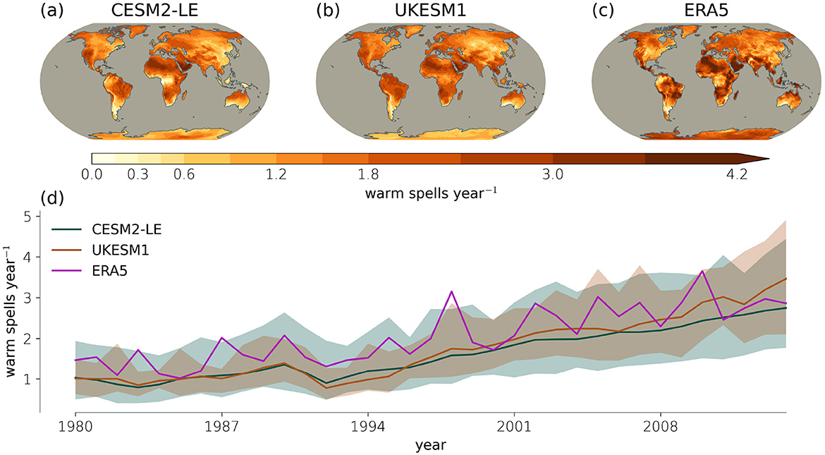
Figure 1. Annual mean warm spell occurrence for 1980–2014 in CESM2, UKESM1 and ERA5, respectively, are shown in (a–c). The time series of annual mean warm spell occurrence area-averaged across all global land grid points is shown in (d). The green line shows the time series for the CESM2-LE, the brown line shows the time series for UKESM1 and the purple line shows the time series for ERA5. The green (brown) shading shows the range of ensemble members in the CESM2-LE (UKESM1).
From a land-only area-averaged perspective, annual mean warm spell event occurrence in ERA5 fits within the range of CESM2-LE and UKESM1 ensemble members, indicating that both models are able to reasonably represent the observed trend in warm spell event frequency from 1980 to 2014 (Figure 1d). The interannual variability of ERA5 is likely larger compared to the CESM2-LE or UKESM1, since both model results are averages across many realizations. Results from similar analyses of warm spell days, duration and amplitude largely agree with the results shown for warm spell occurrence (Supplementary Figures S2–S4). One discrepancy is that, in the CESM2-LE, area averaged ensemble mean warm spell amplitude is ~0.5°C less than that in ERA5 and the UKESM1 historical simulations (Supplementary Figures S4). However, the ERA5 values fit within the range of the CESM2-LE ensemble members.
3 Results
3.1 Characterizing warm spells in current and future climates
A challenge in comparing future projections of warm spells and their characteristics under SSP2–4.5 between CESM2 and UKESM1 is that the magnitude of global temperature change over the simulation period is larger in UKESM1 (as discussed above). In order to address this challenge, we normalize future changes in warm spells and their characteristics by the corresponding global mean temperature change in each model. Changes to warm spell characteristics are overall larger in magnitude in UKESM1 than in CESM2 under SSP2–4.5 (Supplementary Figures S5–S8) before normalization, whereas the magnitude of change is more comparable between models after normalization (Figures 2–5). While this method appears to reasonably account for the differences in future projections of warm spells and their characteristics between models, it assumes that these characteristics increase linearly with temperature. Given that shifts in the mean temperature have been shown to be the dominant contributor to changes in hot extremes (e.g., McKinnon et al., 2016; Seneviratne et al., 2021; Van Loon and Thompson, 2023), this is likely an appropriate assumption. Normalization was not applied to the SAI simulations since the deployment goals in both models are to stabilize global mean temperature (Henry et al., 2023; Richter et al., 2022).
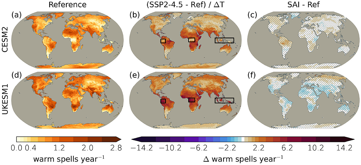
Figure 2. Annual mean warm spell event occurrence is shown for 2020–2039 in CESM2 (a) and 2014–2033 in UKESM1 (d). The change in annual mean warm spell event occurrence for 2060–2069 relative to each model's reference period under SSP2–4.5 normalized by the corresponding change in global mean temperature in CESM2 (1.011°C) and UKESM1 (1.797°C) is shown in (b) and (e), respectively. Annual mean warm spell event occurrence for 2060-2069 relative to each model's reference period under SAI is shown in (c, f). The black boxes in (b) and (e) indicate regions where future projections of warm spells between CESM2 and UKESM1 are distinct. Stippled regions indicate those where the 2060–2069 period is not statistically significantly different from the respective model's reference period according to a two-sample student's t-test with α = 0.05. Each ensemble member is considered to be an independent sample. Multiple testing issues and spatial correlation are accounted for by adjusting the p-value according to the methods described in Wilks (2016).
Over the reference period (2020–2039 in CESM2, 2014–2033 in UKESM1), warm spells occur, on average, up to approximately three times per year over many land regions in both models (Figures 2a, d). Warm spell occurrence, however, exhibits considerable spatial heterogeneity, with more frequent occurrence over regions such as the western United States (U.S.), the Sahara and the Indian subcontinent, and less frequent occurrence over regions such as the eastern U.S., southern Australia and central Asia. Under SSP2–4.5, warm spell occurrence is projected to increase globally by the end of the simulation period (i.e., the 2060s), except over Iceland in CESM2, with increases of up to 10 warm spells per year (Figures 2b, e). Increases in warm spell frequency are largest at lower latitudes over regions such as the Amazon, central Africa and southeast Asia, although increases are up to five warm spells per year over Northern Hemisphere high latitudes (Figures 2b, e). There are some regions where future projections of warm spells are noticeably different between the two models, such as over western North America (Figures 2b, e) and some tropical rainforests (boxed regions in Figures 2b, e). When SAI is deployed, future increases in warm spells are reduced globally (Figures 2c, f). In CESM2, there is little change in warm spell event occurrence between the 2060s under SAI and the reference period, with the largest change being a slight increase (no more than four warm spells per year) over west-central South America (Figure 2c). In contrast, in UKESM1, there is a slight decrease in warm spell occurrence relative to the reference period over most land regions (Figure 2f). To evaluate if changes in warm spell characteristics are significant, we use a two-sample student's t-test at the α = 0.05 level, with the p-value adjusted at each grid point to account for multiple-testing and spatial correlation issues (Wilks, 2016). Each individual ensemble member is considered to be an independent sample. Stippled regions in Figure 2 and all following figures indicate areas where the 2060–2069 period was not found to be statistically significantly different from the reference period of each respective model.
The regions where warm spells occur most frequently (Figures 2a, d) are also the regions where the number of warm spell days is greatest during the reference period (Figures 3a, d). Up to 33 warm spell days occur across all warm spell events per year during this period. Similar to with warm spell occurrence, warm spell days are projected to increase by several times relative to the reference period under SSP2–4.5, with increases of up to 175 warm spell days per year over low latitude regions (Figures 3b, e). There are also similar differences between CESM2 and UKESM1 as with warm spell frequency: for example, there are relatively small increases in warm spell days over tropical rainforests in CESM2 but relatively large increases in UKESM1 (Figures 3b, e). SAI deployment reduces future increases in warm spell days in CESM2 and UKESM1 across the globe such that increases are less than 50 warm spell days per year (Figures 3c, d).
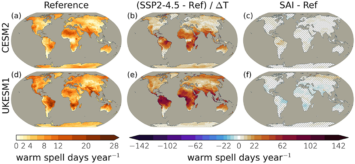
Figure 3. Annual mean warm spell days for 2020–2039 in CESM2 is shown in (a) and 2014–2033 in UKESM1 is shown in (d). The change in annual mean warm spell days for 2060–2069 relative to each model's reference period under SSP2–4.5 normalized by the corresponding change in global mean temperature in CESM2 (1.011°C) and UKESM1 (1.797°C) is shown in (b) and (e), respectively. Annual mean warm spell days for 2060–2069 relative to each model's reference period under SAI is shown in (c, f). Stippled regions indicate those where the 2060–2069 period is not statistically significantly different from the respective model's reference period according to a two-sample student's t-test with α = 0.05. Each ensemble member is considered to be an independent sample. Multiple testing issues and spatial correlation are accounted for by adjusting the p-value according to the methods described in Wilks (2016).
The longest warm spells are generally <10 days in length during the reference period (Figures 4a, d). In UKESM1, warm spell duration reaches up to 108 days over the northern half of South America, which is long compared to the rest of the globe and to CESM2 (Figure 4d). Under SSP2–4.5, warm spell duration is projected to increase as for warm spell occurrence and warm spell days (Figures 4b, e). These increases are reduced under SAI (Figures 4c, f). Differences between CESM2 and UKESM1 for future warm spell duration changes under SSP2–4.5 and SAI are similar to those described for warm spell occurrence and warm spell days. Over west-central South America, there is a larger magnitude reduction in warm spell duration under SAI in UKESM1 compared with changes in warm spell occurrence and warm spell days (Figure 4f). This same region has higher warm spell duration in the reference period compared to other global land areas (Figure 4d).
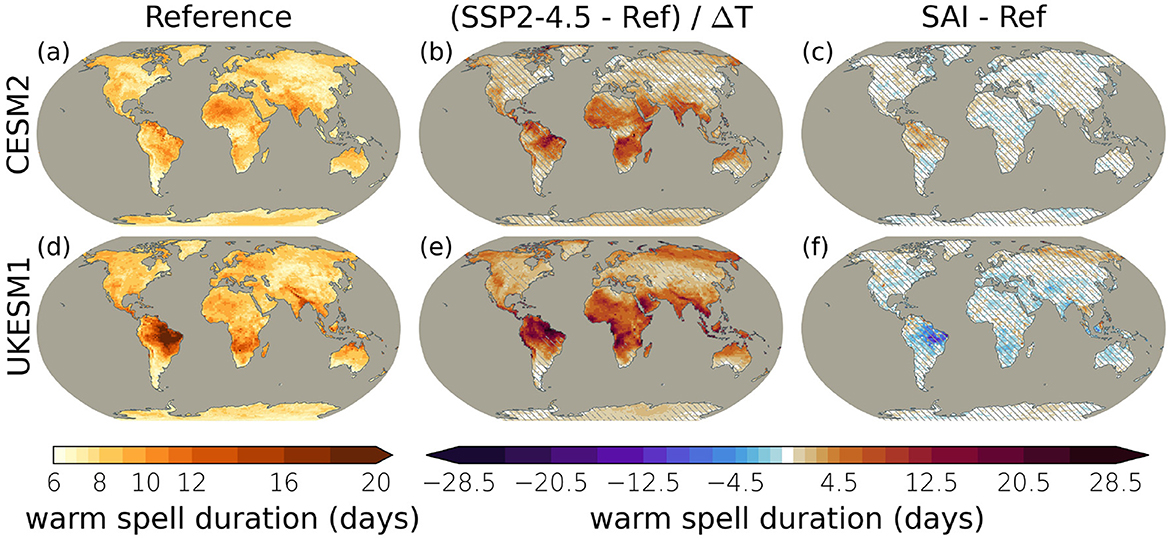
Figure 4. Annual mean warm spell duration (in days) is shown for 2020–2039 in CESM2 (a) and 2014–2033 in UKESM1 (d). The change in annual mean warm spell duration for 2060–2069 relative to each model's reference period under SSP2–4.5 normalized by the corresponding change in global mean temperature in CESM2 (1.011°C) and UKESM1 (1.797°C) is shown in (b) and (e), respectively. Annual mean warm spell duration for 2060–2069 relative to each model's reference period under SAI is shown in (c, f). Note that years without a warm spell were excluded from this portion of analysis. Stippled regions indicate those where the 2060–2069 period is not statistically significantly different from the respective model's reference period according to a two-sample student's t-test with α = 0.05. Each ensemble member is considered to be an independent sample. Multiple testing issues and spatial correlation are accounted for by adjusting the p-value according to the methods described in Wilks (2016).
Warm spell amplitude shows a considerably different spatial pattern in each model's reference period compared to other warm spell characteristics (Figures 5a, d). Warm spell amplitude is largest at high latitudes and smallest at low latitudes, likely because high latitude regions have more temperature variability than lower latitudes (Supplementary Figure S9). Under SSP2–4.5, warm spell amplitude is projected to increase over nearly all global land areas, with increases of up to 8°C (Figures 5b, e). The relative magnitude of increase in amplitude is more spatially homogeneous in both models compared with other warm spell characteristics (Figures 5b, e). When SAI is deployed, the large-scale increase in warm spell amplitude is mostly avoided (Figures 5c, f). However, spatially heterogeneous changes in warm spell amplitude still exist. Some of these regions show contrasting responses between models when SAI is deployed. For instance, CESM2 projects a decrease in warm spell amplitude over Greenland while UKESM1 projects an increase in warm spell amplitude (Figures 5c, f).
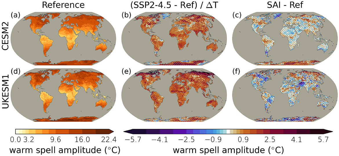
Figure 5. Annual mean warm spell amplitude (in °C) is shown for 2020–2039 in CESM2 (a) and 2014–2033 in UKESM1 (d). The change in annual mean warm spell amplitude for 2060–2069 relative to each model's reference period under SSP2–4.5 normalized by the corresponding change in global mean temperature in CESM2 (1.011°C) and UKESM1 (1.797°C) is shown in (b) and (e), respectively. Annual mean warm spell amplitude for 2060–2069 relative to each model's reference period under SAI is shown in (c, f). Note that years without a warm spell were excluded from this portion of the analysis. Stippled regions indicate those where the 2060–2069 period is not statistically significantly different from the respective model's reference period according to a two-sample student's t-test with α = 0.05. Each ensemble member is considered to be an independent sample. Multiple testing issues and spatial correlation are accounted for by adjusting the p-value according to the methods described in Wilks (2016).
The presented results focus on changes in warm spell characteristics calculated annually, but seasonal analyses were also completed for warm spell occurrence (Figure 6) and other characteristics (not shown). Seasonal warm spell occurrence was calculated assuming seasons are exclusive of one another, meaning that a warm spell is only counted if it reaches the minimum length requirement in the season in which it started. In order to only consider seasons with consecutive months, the first winter season of each analysis period excludes December, and we also omit the last December of each simulation period. Over each model's reference period, the spatial pattern of seasonal warm spell occurrence is relatively similar to annual warm spell occurrence (Figures 2a, d), where warm spells occur more frequently (in excess of 0.4 warm spells per season) over regions such as the western U.S., the Sahara and the Indian subcontinent, and less frequently (fewer than 0.2 warm spells per season) over regions such as the eastern U.S. and southern Australia (Figure 6). There are some regions where there is notable seasonal variability including over the Amazon and west-central Africa (Figure 6). Over the Amazon, seasonal variability is most apparent in CESM2, where warm spells occur more frequently in the northern portion during December, January and February (DJF), and more frequently over the southern portion during June, July, and August (JJA) (Figure 6). Over west-central Africa, broadly speaking, warm spells occur rarely or not at all throughout the year (Figure 6). This region of low occurrence expands northward during JJA and September, October, and November (SON). Seasonal variability is more evident over west-central Africa in UKESM1 than that over the Amazon. However, there is generally less seasonal variability and more frequent warm spells over this region in UKESM1 than in CESM2 (Figure 6). Although not as stark, regions such as the southeastern U.S., western Europe and northeast Russia all exhibit seasonal variability as well (Figure 6). While not shown, future projections of warm spell occurrence calculated from a seasonal perspective have similar spatial patterns to those of the reference period. Further, warm spell days and duration calculated seasonally are consistent with those for warm spell occurrence. This follows for seasonal warm spell amplitude, although warm spell amplitude tends to be larger in the summer hemisphere.
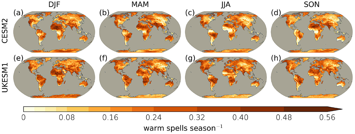
Figure 6. Seasonal warm spell event occurrence is shown for 2020–2039 in CESM2 for December, January and February (DJF) (a), March, April and May (MAM) (b), June, July and August (JJA) (c) and September, October and November (SON) (d). Seasonal warm spell event occurrence is shown for 2014–2033 in UKESM1 for DJF (e), MAM (f), JJA (g), and SON (h).
3.2 Physical factors that drive the differences between CESM2 and UKESM1
The dominant factor contributing to future projections of warm spells and their characteristics is changes to global mean temperature: warm spell characteristics increase globally in CESM2 and UKESM1 under SSP2–4.5, but change little in the simulations when SAI was deployed (Figures 2–5). This relationship has been shown in the observational record (McKinnon et al., 2016), reanalysis (Van Loon and Thompson, 2023), and model projections (Sillmann et al., 2013). A second factor contributing to differences between CESM2 and UKESM1 is the spatial pattern of warming. In UKESM1, there is projected to be a slight decrease in warm spell occurrence, days and duration across most global land areas (Figures 2f, 3f, 4f) in the simulations with SAI. This is likely due to the spatial pattern of temperature change, where temperature increases in the Arctic, and most other regions cool slightly in order to reach the global mean temperature target of SAI deployment (Figure 7f). The region of cooling that is projected over the North Atlantic in CESM2 is another example of how the spatial pattern of warming contributes to future projections of warm spells (Figures 7b, c). Small regions over northeastern Canada, southern Greenland and northwestern Europe that are adjacent to this cooling region are projected to have nearly no change or slight decreases in warm spell characteristics (Figures 2b, c, 3b, c, 4b, c, 5b, c). The differences in the response of the Arctic and the North Atlantic to rising greenhouse gas concentrations between CESM2 and UKESM1 may be due to how Arctic sea ice and resulting land-atmosphere interactions and the Atlantic meridional overturning circulation, respectively, are represented in each model. Confirming these relationships is beyond the scope of this work.
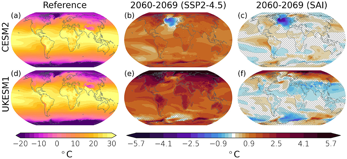
Figure 7. Annual mean 2 m temperature (in °C) is shown for 2020–2039 in CESM2 (a) and 2014–2033 in UKESM1 (d). The change in annual mean 2 m temperature for 2060–2069 relative to each model's reference period under SSP2–4.5 is shown in (b) and (e), respectively. Annual mean 2 m temperature for 2060–2069 relative to each model's reference period under SAI is shown in (c, f). Stippled regions indicate those where the 2060–2069 period is not statistically significantly different from the respective model's reference period according to a two-sample student's t-test with α = 0.05. Each ensemble member is considered to be an independent sample. Multiple testing issues and spatial correlation are accounted for by adjusting the p-value according to the methods described in Wilks (2016).
There are additional differences in future projections of warm spell characteristics between the two models that are not explained by the magnitude of mean warming or the spatial pattern of temperature change. CESM2 projects larger increases in warm spell occurrence, days and duration over western North America under SSP2–4.5 than in UKESM1 (Figures 2–4). There are also prominent differences between models over tropical rainforests (boxed regions in Figures 2b, e, 3b, e, 4b, e), where smaller magnitude increases in warm spell characteristics are projected in CESM2 than UKESM1. These respective differences may be due to differences in other factors important for warm spell characteristics, such as inter-model differences in future projections of large-scale atmospheric circulation patterns, soil-moisture fluctuations and land cover properties (e.g., Benson and Dirmeyer, 2021; Domeisen et al., 2023; Kautz et al., 2022; Seneviratne et al., 2010; Skinner et al., 2018). Next, we examine the physical mechanisms that may be responsible for the differences in future projections of warm spell characteristics over tropical rainforests (land regions in black boxes in Figure 2b), since these are the largest differences that occur between the two models under SSP2–4.5.
3.2.1 Tropical rainforests
We use leaf area index (LAI) to evaluate how changes to plant physiology may influence future projections of warm spells over tropical rainforests, given that plant physiological changes have been shown to affect both regional temperature projections (Zarakas et al., 2020) and the incidence of extremes (Skinner et al., 2018). LAI is the ratio of one-sided green leaf area per unit horizontal ground surface area (Fang et al., 2019) and may increase due to higher productivity under elevated CO2 concentrations. LAI is output by the land component of CESM2, the Community Land Model, version 5 (CLM5; Lawrence et al., 2019), and the land component of UKESM1, the Joint U.K. Land Environment Simulator (JULES; Clark et al., 2011), respectively. In the reference period, regions with high LAI are similar between models, though the extent of these regions is larger in UKESM1 (Figures 8a, d). LAI is projected to increase under SSP2–4.5 over tropical rainforests in CESM2 by up to 1.75 m2 m−2 (blacked boxed regions in Figure 8b). In contrast, LAI is projected to change very little (increase by no more than 0.37 m2 m−2) over these same regions in UKESM1 (black boxed regions in Figure 8e). When SAI is deployed, LAI changes are similar to those under SSP2–4.5, although increases are larger over tropical rainforests under SAI in UKESM1 than under SSP2–4.5 (Figures 8c, f).
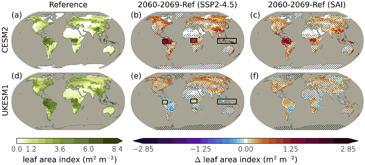
Figure 8. Annual mean leaf area index is shown for 2020–2039 in CESM2 (a) and 2014–2033 in UKESM1 (d). The change in annual mean leaf area index for 2060–2069 relative to each model's reference period under SSP2–4.5 is shown in (b) and (e), respectively. Annual mean leaf area index for 2060–2069 relative to each model's reference period under SAI is shown in (c, f). Stippled regions indicate those where the 2060–2069 period is not statistically significantly different from the respective model's reference period according to a two-sample student's t-test with α = 0.05. Each ensemble member is considered to be an independent sample. Multiple testing issues and spatial correlation are accounted for by adjusting the p-value according to the methods described in Wilks (2016).
The discrepancies in future projections of LAI between models may be due to differing responses of plant physiology to climate change under SSP2–4.5 as simulated by CLM5 and JULES. CO2 fertilization, where photosynthesis increases in response to rising atmospheric CO2 concentrations (Donohue et al., 2013; Kirschbaum, 2004), as well as stomatal closure, where the pores which regulate the exchange of water and CO2 into and out of the leaf, close as atmospheric CO2 concentration rise (Ainsworth and Rogers, 2007; Field et al., 1995), are processes contributing to the plant physiological response to climate change. As a result of CO2 fertilization, productivity (biomass production) typically increases which leads to increased canopy transpiration. Stomatal closure generally leads to declines in leaf level transpiration. The rate of photosynthesis is also sensitive to temperature, increasing until optimal temperature levels are reached (Kirschbaum, 2004; Kirschbaum and McMillan, 2018), although acclimation is possible (Yamori et al., 2014). One difference between CLM5 and JULES is that CLM5 includes a parameterization that allows for photosynthetic acclimation (Lombardozzi et al., 2015), while the version of JULES used does not (Clark et al., 2011; Harper et al., 2016, 2018). The inclusion of acclimation in CLM5 may thus be a cause for the disagreement between models for future projections of LAI since acclimation can increase the productivity of plants at higher temperatures. Increased LAI is connected with increased transpiration and evaporative cooling, which could explain why there are small changes in warm spell occurrence, days and duration in CESM2 compared to UKESM1, where LAI doesn't appreciably change under SSP2–4.5 over tropical rainforests (Figures 2b, e, 3b, e, 4b, e). Time series analysis of evaporative fraction over tropical rainforest regions supports these arguments (see Supplementary material and Supplementary Figure S10).
4 Conclusion
We have assessed warm spell characteristics in the context of climate change under SSP2–4.5 with and without the deployment of SAI in CESM2 and UKESM1. In the current climate, warm spells occur up to three times per year and exhibit a heterogeneous spatial pattern (Figures 2–5). When evaluating warm spells seasonally, the spatial pattern is generally similar to annual warm spell occurrence, although some regions exhibit distinct seasonality, such as over the Amazon and west-central Africa (Figure 6). Warm spells and associated characteristics are projected to increase globally in both models under SSP2–4.5. These increases are reduced when SAI is deployed. While the representation of warm spells is similar, overall, between CESM2 and UKESM1 in current and future climates, distinct differences exist. One principal difference is that the relative magnitude of increase in warm spell occurrence, days, duration and amplitude is larger in UKESM1 than in CESM2 (Supplementary Figures S5–S8), likely because UKESM1 has a higher ECS than CESM2 (Zelinka et al., 2020). Additionally, in UKESM1, warm spell occurrence, days and duration are projected to decrease slightly under SAI. This is likely due to the spatial pattern of temperature change in UKESM1, where temperature increases in the Arctic, and most other regions cool slightly in order to reach the temperature targets of SAI deployment (Figure 7). These results indicate that changes in mean temperature as well as the spatial pattern of change are the dominant contributors to future changes in warm spell event occurrence, days, duration and amplitude regardless of if SAI is deployed or not, which agrees with previous work (e.g., McKinnon et al., 2016; Seneviratne et al., 2021; Van Loon and Thompson, 2023).
There also exists notable differences in future projections of warm spells over tropical rainforests between the two models. Over these regions, CESM2 projects a relatively small increase in warm spell occurrence, days and duration under CESM2, whereas UKESM1 projects a relatively large magnitude increase (Figures 2b, e, 3b, e, 4b, e). Contrasting plant physiological responses to increasing CO2 and temperature over these regions is likely to contribute to these differences; namely, LAI is projected to increase under SSP2–4.5 much more in CESM2 than in UKESM1 (Figure 8). It is important to note that both models contain biases in their representation of LAI. Song et al. (2021) compared the representation of LAI in CMIP6 models to several observational datasets and indicated that the recent historical (1982–2014) average LAI more closely resembled observations in CESM2 than in UKESM1. Specifically, UKESM1 overestimates the magnitude and extent of regions of high LAI in tropical rainforests, especially over the Amazon. However, the trend in LAI over the historical period was overestimated in CESM2 and underestimated in UKESM1 over these regions, with the trend in UKESM1 being closer to observations (Song et al., 2021).
We have highlighted potential sources of inter-model uncertainty and model bias that can impact the magnitude and spatial distribution of future projections of warm spells, an important aspect of uncertainty for climate prediction (Hawkins and Sutton, 2009). We found that the spatial pattern and magnitude of warming, which differ between CESM2 and UKESM1, is a dominant factor contributing to future projections of warm spells and associated characteristics. We also found that contrasting future projections of warm spells over tropical rainforests between the two models may be due, in part, to differences in how plant physiology responds to increasing atmospheric CO2 and temperature. In particular, differences in how these responses are parameterized in CLM5 and JULES are likely critical: CLM5 includes consideration of the acclimation of photosynthesis, while JULES, to our knowledge, does not. We highlighted several sources of uncertainty that exist between CESM2 and UKESM1 and emphasize the importance of inter-model comparisons in climate change research. Future analyses could be extended to include additional ESMs in order to more fully capture the range of inter-model uncertainty.
Other avenues for future exploration are the potential impact of internal climate variability and the sensitivity to the chosen future scenario on warm spell characteristics. Both have been shown to have a meaningful effect on future climate projections (Deser et al., 2020; Hawkins and Sutton, 2009; Schwarzwald and Lenssen, 2022) and future projections of extreme heat events (Perkins and Alexander, 2013; Perkins-Kirkpatrick and Gibson, 2017; Sillmann et al., 2013). Future work could also explore the impact of other physical processes known to impact extremes, such as those related to large-scale circulation patterns, soil-moisture fluctuations, cloud cover and land cover properties (Benson and Dirmeyer, 2021; Domeisen et al., 2023; Kautz et al., 2022; Seneviratne et al., 2010; Sousa et al., 2018). These processes can be particularly impactful at the regional scale, and likely contribute to the spatial heterogeneity of warm spell occurrence in future projections, as well as to differences between models. Finally, the results of analyses such as ours are also dependent on the specific warm spell definition and the choice of base period.
While the extent to which SAI may be able to mitigate future increases in indices of extremes has been assessed previously (Tye et al., 2022), to our knowledge, this is the first study to assess globally future projections of warm spells and their characteristics under both climate change and SAI using two different ESMs. Compared to heatwaves, which occur only in the warm season, warm spells, which occur throughout the year, have received considerably less attention. We found that over most land regions, warm spells are not concentrated in only the warm season (Figure 6). The impact that warm spells in other seasons could have on ecosystem vulnerability and water resource management (Hansen et al., 2014; Scaff et al., 2024), for instance, underscores the importance of extending analyses beyond just warm season events. We found that under SSP2–4.5, warm spell occurrence, days, duration and amplitude are expected to increase by up to several times their reference period values (Figures 2–5), suggesting that impacts will also increase, such as those on human mortality and morbidity (Anderson and Bell, 2009; Dagon and Schrag, 2017; Guirguis et al., 2014; Matthews et al., 2025), agricultural yields (Bezner Kerr and Gawa, 2023; Brás et al., 2021) and energy demand (Auffhammer et al., 2017). The deployment of SAI could reduce many of these impacts.
Data availability statement
The original contributions presented in the study are included in the article/Supplementary material, further inquiries can be directed to the corresponding author.
Author contributions
IG: Conceptualization, Data curation, Formal analysis, Investigation, Methodology, Project administration, Software, Validation, Visualization, Writing – original draft, Writing – review & editing. JH: Funding acquisition, Methodology, Project administration, Resources, Supervision, Writing – review & editing. DL: Methodology, Writing – review & editing.
Funding
The author(s) declare that financial support was received for the research and/or publication of this article. This work was supported by the National Oceanic and Atmospheric Administration (NOAA Grant NA22OAR4320473).
Acknowledgments
The ARISE-SAI simulations were produced by the National Center for Atmospheric Research (NCAR) with support from the National Science Foundation (NSF; Grant 1852977) and by SilverLining through its Safe Climate Research Initiative. The CESM2 Large Ensemble simulations were produced by NCAR. The CESM project is supported primarily by NSF. The UKESM1 SAI simulations were produced by Mohit Dalvi and Andy Jones at the U.K. Met Office Hadley Centre. The UKESM1 SSP2–4.5 and historical simulations were produced by the U.K. Met Office Hadley Centre as a part of CMIP6. The authors extend special thanks to Peter Cox for his insightful comments on the early stages of this work, especially related to the influence of land-atmosphere interactions on temperature and warm spells. The authors also thank Matthew Henry and Lina Mercado for their expertise on the UKESM1 model and simulations. Finally, the authors thank the two reviewers, Isobel Parry and Romaric Odoulami, for their thoughtful comments on the manuscript.
Conflict of interest
The authors declare that the research was conducted in the absence of any commercial or financial relationships that could be construed as a potential conflict of interest.
Generative AI statement
The author(s) declare that no Gen AI was used in the creation of this manuscript.
Publisher's note
All claims expressed in this article are solely those of the authors and do not necessarily represent those of their affiliated organizations, or those of the publisher, the editors and the reviewers. Any product that may be evaluated in this article, or claim that may be made by its manufacturer, is not guaranteed or endorsed by the publisher.
Supplementary material
The Supplementary Material for this article can be found online at: https://www.frontiersin.org/articles/10.3389/fclim.2025.1581305/full#supplementary-material
References
Ainsworth, E. A., and Rogers, A. (2007). The response of photosynthesis and stomatal conductance to rising [CO2]: mechanisms and environmental interactions. Plant Cell Environ. 30, 258–270. doi: 10.1111/j.1365-3040.2007.01641.x
Anderson, B. G., and Bell, M. L. (2009). Weather-related mortality: how heat, cold, and heat waves affect mortality in the United States. Epidemiology 20, 205–213. doi: 10.1097/EDE.0b013e318190ee08
Archibald, A. T., O'Connor, F. M., Abraham, N. L., Archer-Nicholls, S., Chipperfield, M. P., Dalvi, M., et al. (2020). Description and evaluation of the UKCA stratosphere-troposphere chemistry scheme (StratTrop vn 1.0) implemented in UKESM1. Geosci. Model Dev. 13, 1223–1266. doi: 10.5194/gmd-13-1223-2020
Auffhammer, M., Baylis, P., and Hausman, C. H. (2017). Climate change is projected to have severe impacts on the frequency and intensity of peak electricity demand across the United States. Proc. Nat. Acad. Sci. 114, 1886–1891. doi: 10.1073/pnas.1613193114
Bednarz, E. M., Visioni, D., Richter, J. H., Butler, A. H., and MacMartin, D. G. (2022). Impact of the latitude of stratospheric aerosol injection on the southern annular mode. Geophys. Res. Lett. 49:e2022GL100353. doi: 10.1029/2022GL100353
Benson, D. O., and Dirmeyer, P. A. (2021). Characterizing the relationship between temperature and soil moisture extremes and their role in the exacerbation of heat waves over the contiguous United States. J. Clim. 34, 2175–2187. doi: 10.1175/JCLI-D-20-0440.1
Brás, T. A., Seixas, J., Carvalhais, N., and Jägermeyr, J. (2021). Severity of drought and heatwave crop losses tripled over the last five decades in Europe. Environ. Res. Lett. 16:065012. doi: 10.1088/1748-9326/abf004
Clark, D. B., Mercado, L. M., Sitch, S., Jones, C. D., Gedney, N., Best, M. J., et al. (2011). The joint UK land environment simulator (JULES), model description - part 2: carbon fluxes and vegetation dynamics. Geosci. Model Dev. 4, 701–722. doi: 10.5194/gmd-4-701-2011
Cooper, R. N., Houghton, J. T., McCarthy, J. J., and Metz, B. (2002). Climate change 2001: the scientific basis. Foreign Aff. 81:208. doi: 10.2307/20033020
Crutzen, P. J. (2006). Albedo enhancement by stratospheric sulfur injections: a contribution to resolve a policy dilemma? Clim. Chang. 77, 211–220. doi: 10.1007/s10584-006-9101-y
Dagon, K., and Schrag, D. P. (2017). Regional climate variability under model simulations of solar geoengineering. J. Geophys. Res. Atmos. 122, 12.106–12.121. doi: 10.1002/2017JD027110
Danabasoglu, G., Lamarque, J., Bacmeister, J., Bailey, D. A., DuVivier, A. K., Edwards, J., et al. (2020). The community earth system model version 2 (CESM2). J. Adv. Model. Earth Syst. 12:e2019MS001916. doi: 10.1029/2019MS001916
DeRepentigny, P., Jahn, A., Holland, M. M., Kay, J. E., Fasullo, J., Lamarque, J.-F., et al. (2022). Enhanced simulated early 21st century Arctic sea ice loss due to CMIP6 biomass burning emissions. Sci. Adv. 8:eabo2405. doi: 10.1126/sciadv.abo2405
Deser, C., Lehner, F., Rodgers, K. B., Ault, T., Delworth, T. L., DiNezio, P. N., et al. (2020). Insights from earth system model initial-condition large ensembles and future prospects. Nat. Clim. Chang. 10, 277–286. doi: 10.1038/s41558-020-0731-2
Domeisen, D. I. V., Eltahir, E. A. B., Fischer, E. M., Knutti, R., Perkins-Kirkpatrick, S. E., Schär, C., et al. (2023). Prediction and projection of heatwaves. Nat. Rev. Earth Environ. 4, 36–50. doi: 10.1038/s43017-022-00371-z
Donohue, R. J., Roderick, M. L., McVicar, T. R., and Farquhar, G. D. (2013). Impact of CO2 fertilization on maximum foliage cover across the globe's warm, arid environments. Geophys. Res. Lett. 40, 3031–3035. doi: 10.1002/grl.50563
Ebi, K. L., Capon, A., Berry, P., Broderick, C., Dear, R. D., Havenith, G., et al. (2021). Hot weather and heat extremes: health risks. Lancet 398, 698–708. doi: 10.1016/S0140-6736(21)01208-3
Eyring, V., Bony, S., Meehl, G. A., Senior, C. A., Stevens, B., Stouffer, R. J., et al. (2016). Overview of the coupled model intercomparison project phase 6 (CMIP6) experimental design and organization. Geosci. Model Dev. 9, 1937–1958. doi: 10.5194/gmd-9-1937-2016
Fang, H., Baret, F., Plummer, S., and Schaepman-Strub, G. (2019). An overview of global leaf area index (LAI): methods, products, validation, and applications. Rev. Geophys. 57, 739–799. doi: 10.1029/2018RG000608
Fasullo, J. T., Lamarque, J.-F., Hannay, C., Rosenbloom, N., Tilmes, S., DeRepentigny, P., et al. (2022). Spurious late historical-era warming in CESM2 driven by prescribed biomass burning emissions. Geophys. Res. Lett. 49:e2021GL097420. doi: 10.1029/2021GL097420
Field, C. B., Jackson, R. B., and Mooney, H. A. (1995). Stomatal responses to increased CO2: implications from the plant to the global scale. Plant Cell Environ. 18, 1214–1225. doi: 10.1111/j.1365-3040.1995.tb00630.x
Fischer, E. M., and Schär, C. (2009). Future changes in daily summer temperature variability: driving processes and role for temperature extremes. Clim. Dyn. 33, 917–935. doi: 10.1007/s00382-008-0473-8
Fischer, E. M., and Schär, C. (2010). Consistent geographical patterns of changes in high-impact European heatwaves. Nat. Geosci., 3, 398–403. doi: 10.1038/ngeo866
Gettelman, A., Mills, M. J., Kinnison, D. E., Garcia, R. R., Smith, A. K., Marsh, D. R., et al. (2019). The whole atmosphere community climate model version 6 (WACCM6). J. Geophys. Res. Atmos. 124, 12380–12403. doi: 10.1029/2019JD030943
Glade, I., Hurrell, J. W., Sun, L., and Rasmussen, K. L. (2023). Assessing the impact of stratospheric aerosol injection on US convective weather environments. Earth's Future 11:e2023EF004041. doi: 10.1029/2023EF004041
Goddard, P. B., Kravitz, B., MacMartin, D. G., Visioni, D., Bednarz, E. M., Lee, W. R., et al. (2023). Stratospheric aerosol injection can reduce risks to antarctic ice loss depending on injection location and amount. J. Geophys. Res. Atmos. 128:e2023JD039434. doi: 10.1029/2023JD039434
Guirguis, K., Gershunov, A., Tardy, A., and Basu, R. (2014). The impact of recent heat waves on human health in California. J. Appl. Meteorol. Climatol. 53, 3–19. doi: 10.1175/JAMC-D-13-0130.1
Hansen, B. B., Isaksen, K., Benestad, R. E., Kohler, J., Pedersen, S., Loe, L. E., et al. (2014). Warmer and wetter winters: characteristics and implications of an extreme weather event in the High Arctic. Environ. Res. Lett. 9:114021. doi: 10.1088/1748-9326/9/11/114021
Harper, A. B., Cox, P. M., Friedlingstein, P., Wiltshire, A. J., Jones, C. D., Sitch, S., et al. (2016). Improved representation of plant functional types and physiology in the Joint UK Land Environment Simulator (JULES v4.2) using plant trait information. Geosci. Model Dev. 9, 2415–2440. doi: 10.5194/gmd-9-2415-2016
Harper, A. B., Wiltshire, A. J., Cox, P. M., Friedlingstein, P., Jones, C. D., Mercado, L. M., et al. (2018). Vegetation distribution and terrestrial carbon cycle in a carbon cycle configuration of JULES4.6 with new plant functional types. Geosci. Model Dev. 11, 2857–2873. doi: 10.5194/gmd-11-2857-2018
Hawkins, E., and Sutton, R. (2009). The potential to narrow uncertainty in regional climate predictions. Bull. Am. Meteorol. Soc. 9, 1095–1108. doi: 10.1175/2009BAMS2607.1
Haywood, J. M., Boucher, O., Lennard, C., Storelvmo, T., Tilmes, S., Visioni, D., et al. (2025). World Climate Research Programme lighthouse activity: an assessment of major research gaps in solar radiation modification research. Front. Clim. 7:1507479. doi: 10.3389/fclim.2025.1507479
Henry, M., Haywood, J., Jones, A., Dalvi, M., Wells, A., Visioni, D., et al. (2023). Comparison of UKESM1 and CESM2 simulations using the same multi-target stratospheric aerosol injection strategy. Atmos. Chem. Phys. 23, 13369–13385. doi: 10.5194/acp-23-13369-2023
Hersbach, H., Bell, B., Berrisford, P., Hirahara, S., Horányi, A., Muñoz-Sabater, J., et al. (2020). The ERA5 global reanalysis. Q. J. R. Meteorol. Soc. 146, 1999–2049. doi: 10.1002/qj.3803
Hueholt, D. M., Barnes, E. A., Hurrell, J. W., and Morrison, A. L. (2024). Speed of environmental change frames relative ecological risk in climate change and climate intervention scenarios. Nat. Commun. 15:3332. doi: 10.1038/s41467-024-47656-z
Huntingford, C., Cox, P. M., Ritchie, P. D. L., Clarke, J. J., Parry, I. M., Williamson, M. S., et al. (2024). Acceleration of daily land temperature extremes and correlations with surface energy fluxes. npj Clim. Atmos. Sci. 7, 1–10. doi: 10.1038/s41612-024-00626-0
Hurrell, J. W., Haywood, J. M., Lawrence, P. J., Lennard, C. J., and Oschlies, A. (2024). Climate intervention research in the World Climate Research Programme: a perspective. Front. Clim. 6:1505860. doi: 10.3389/fclim.2024.1505860
IPCC (2021). Climate Change 2021- The Physical Science Basis: Working Group I Contribution to the Sixth Assessment Report of the Intergovernmental Panel on Climate Change, 1 Edn. Cambridge: Cambridge University Press.
IPCC (2022). Global Warming of 1.5°C: IPCC Special Report on Impacts of Global Warming of 1.5°C above Pre-industrial Levels in Context of Strengthening Response to Climate Change, Sustainable Development, and Efforts to Eradicate Poverty, 1 Edn. Cambridge: Cambridge University Press. doi: 10.1017/9781009157940
Jiang, J., Xia, Y., Cao, L., Kravitz, B., MacMartin, D. G., Fu, J., et al. (2024). Different strategies of stratospheric aerosol injection would significantly affect climate extreme mitigation. Earth's Future 12:e2023EF004364. doi: 10.1029/2023EF004364
Jones, A. D., Rastogi, D., Vahmani, P., Stansfield, A. M., Reed, K. A., Thurber, T., et al. (2023). Continental United States climate projections based on thermodynamic modification of historical weather. Sci. Data 10:664. doi: 10.1038/s41597-023-02485-5
Kautz, L.-A., Martius, O., Pfahl, S., Pinto, J. G., Ramos, A. M., Sousa, P. M., et al. (2022). Atmospheric blocking and weather extremes over the Euro-Atlantic sector - a review. Weather Clim. Dyn. 3, 305–336. doi: 10.5194/wcd-3-305-2022
Kerr, B., and Gawa, H. (2023). Climate Change 2022 - Impacts, Adaptation and Vulnerability: Working Group II Contribution to the Sixth Assessment Report of the Intergovernmental Panel on Climate Change, 1 Edn. Cambridge: Cambridge University Press.
Keys, P. W., Barnes, E. A., Diffenbaugh, N. S., Hurrell, J. W., and Bell, C. M. (2022). Potential for perceived failure of stratospheric aerosol injection deployment. Proc. Nat. Acad. Sci. 119:e2210036119. doi: 10.1073/pnas.2210036119
Kirschbaum, M. U. F. (2004). Direct and indirect climate change effects on photosynthesis and transpiration. Plant Biol. 6, 242–253. doi: 10.1055/s-2004-820883
Kirschbaum, M. U. F., and McMillan, A. M. S. (2018). Warming and elevated CO2 have opposing influences on transpiration. Which is more important? Curr. For. Rep. 4, 51–71. doi: 10.1007/s40725-018-0073-8
Kravitz, B., MacMartin, D. G., Mills, M. J., Richter, J. H., Tilmes, S., Lamarque, J.-F., et al. (2017). First simulations of designing stratospheric sulfate aerosol geoengineering to meet multiple simultaneous climate objectives. J. Geophys. Res. Atmos. 122, 12.616–12.634. doi: 10.1002/2017JD026874
Kravitz, B., Robock, A., Boucher, O., Schmidt, H., Taylor, K. E., Stenchikov, G., et al. (2011). The geoengineering model intercomparison project (GeoMIP). Atmos. Sci. Lett. 12, 162–167. doi: 10.1002/asl.316
Lawrence, D. M., Fisher, R. A., Koven, C. D., Oleson, K. W., Swenson, S. C., Bonan, G., et al. (2019). The community land model version 5: description of new features, benchmarking, and impact of forcing uncertainty. J. Adv. Model. Earth Syst. 11, 4245–4287. doi: 10.1029/2018MS001583
Lee, W. R., MacMartin, D. G., Visioni, D., Kravitz, B., Chen, Y., Moore, J. C., et al. (2023). High-latitude stratospheric aerosol injection to preserve the arctic. Earth's Future 11:e2022EF003052. doi: 10.1029/2022EF003052
Lombardozzi, D. L., Bonan, G. B., Smith, N. G., Dukes, J. S., and Fisher, R. A. (2015). Temperature acclimation of photosynthesis and respiration: a key uncertainty in the carbon cycle-climate feedback. Geophys. Res. Lett. 42, 8624–8631. doi: 10.1002/2015GL065934
Lorenz, R., Argüeso, D., Donat, M. G., Pitman, A. J., van den Hurk, B., Berg, A., et al. (2016). Influence of land-atmosphere feedbacks on temperature and precipitation extremes in the GLACE-CMIP5 ensemble. J. Geophys. Res. Atmos. 121, 607–623. doi: 10.1002/2015JD024053
MacMartin, D. G., Kravitz, B., Keith, D. W., and Jarvis, A. (2014). Dynamics of the coupled human-climate system resulting from closed-loop control of solar geoengineering. Clim. Dyn. 43, 243–258. doi: 10.1007/s00382-013-1822-9
Matthews, H. D., and Wynes, S. (2022). Current global efforts are insufficient to limit warming to 1.5°C. Science 376, 1404–1409. doi: 10.1126/science.abo3378
Matthews, T., Raymond, C., Foster, J., Baldwin, J. W., Ivanovich, C., Kong, Q., et al. (2025). Mortality impacts of the most extreme heat events. Nat. Rev. Earth Environ. 6, 193–210. doi: 10.1038/s43017-024-00635-w
McKinnon, K. A., Rhines, A., Tingley, M. P., and Huybers, P. (2016). The changing shape of Northern Hemisphere summer temperature distributions. J. Geophys. Res. Atmos. 121, 8849–8868. doi: 10.1002/2016JD025292
Meehl, G. A., Boer, G. J., Covey, C., Latif, M., and Stouffer, R. J. (1997). Intercomparison makes for a better climate model. Eos Trans. Am. Geophys. Union 78, 445–451. doi: 10.1029/97EO00276
Meehl, G. A., Zwiers, F., Evans, J., Knutson, T., Mearns, L., Whetton, P., et al. (2000). Trends in extreme weather and climate events: issues related to modeling extremes in projections of future climate change. Bull. Am. Meteorol. Soc. 78, 445–451. doi: 10.1175/1520-0477(2000)081<0427:TIEWAC>2.3.CO;2
Morrison, A. L., Barnes, E. A., and Hurrell, J. W. (2024). Stratospheric aerosol injection to stabilize northern hemisphere terrestrial permafrost under the ARISE-SAI-1.5 scenario. Earth's Future 12:e2023EF004151. doi: 10.1029/2023EF004151
Mueller, N. D., Butler, E. E., McKinnon, K. A., Rhines, A., Tingley, M., Holbrook, N. M., et al. (2016). Cooling of US Midwest summer temperature extremes from cropland intensification. Nat. Clim. Chang. 6, 317–322. doi: 10.1038/nclimate2825
Obahoundje, S., Nguessan-Bi, V. H., Diedhiou, A., Kravitz, B., and Moore, J. C. (2023). Implication of stratospheric aerosol geoengineering on compound precipitation and temperature extremes in Africa. Sci. Total Environ. 863:160806. doi: 10.1016/j.scitotenv.2022.160806
O'Neill, B. C., Kriegler, E., Ebi, K. L., Kemp-Benedict, E., Riahi, K., Rothman, D. S., et al. (2017). The roads ahead: narratives for shared socioeconomic pathways describing world futures in the 21st century. Glob. Environ. Change 42, 169–180. doi: 10.1016/j.gloenvcha.2015.01.004
Perkins, S. E., and Alexander, L. V. (2013). On the measurement of heat waves. J. Clim. 26, 4500–4517. doi: 10.1175/JCLI-D-12-00383.1
Perkins, S. E., Alexander, L. V., and Nairn, J. R. (2012). Increasing frequency, intensity and duration of observed global heatwaves and warm spells. Geophys. Res. Lett. 39. doi: 10.1029/2012GL053361
Perkins-Kirkpatrick, S. E., and Gibson, P. B. (2017). Changes in regional heatwave characteristics as a function of increasing global temperature. Sci. Rep. 7:12256. doi: 10.1038/s41598-017-12520-2
Riahi, K., van Vuuren, D. P., Kriegler, E., Edmonds, J., O'Neill, B. C., Fujimori, S., et al. (2017). The shared socioeconomic pathways and their energy, land use, and greenhouse gas emissions implications: an overview. Glob. Environ. Change 42, 153–168. doi: 10.1016/j.gloenvcha.2016.05.009
Richter, J. H., Visioni, D., MacMartin, D. G., Bailey, D. A., Rosenbloom, N., Dobbins, B., et al. (2022). Assessing responses and impacts of solar climate intervention on the Earth system with stratospheric aerosol injection (ARISE-SAI): protocol and initial results from the first simulations. Geosci. Model Dev. 15, 8221–8243. doi: 10.5194/gmd-15-8221-2022
Rodgers, K. B., Lee, S.-S., Rosenbloom, N., Timmermann, A., Danabasoglu, G., Deser, C., et al. (2021). Ubiquity of human-induced changes in climate variability. Earth Syst. Dyn. 12, 1393–1411. doi: 10.5194/esd-12-1393-2021
Scaff, L., Krogh, S. A., Musselman, K., Harpold, A., Li, Y., Lillo-Saavedra, M., et al. (2024). The impacts of changing winter warm spells on snow ablation over western North America. Water Resour. Res. 60:e2023WR034492. doi: 10.1029/2023WR034492
Schär, C., Vidale, P. L., Lüthi, D., Frei, C., Häberli, C., Liniger, M. A., et al. (2004). The role of increasing temperature variability in European summer heatwaves. Nature 427, 332–336. doi: 10.1038/nature02300
Schleussner, C.-F., Rogelj, J., Schaeffer, M., Lissner, T., Licker, R., Fischer, E. M., et al. (2016). Science and policy characteristics of the Paris Agreement temperature goal. Nat. Clim. Chang. 6, 827–835. doi: 10.1038/nclimate3096
Schwarzwald, K., and Lenssen, N. (2022). The importance of internal climate variability in climate impact projections. Proc. Nat. Acad. Sci. 119:e2208095119. doi: 10.1073/pnas.2208095119
Sellar, A. A., Jones, C. G., Mulcahy, J. P., Tang, Y., Yool, A., Wiltshire, A., et al. (2019). UKESM1: description and evaluation of the U.K. earth system model. J. Adv. Model. Earth Syst. 11, 4513–4558. doi: 10.1029/2019MS001739
Seneviratne, S. I., Corti, T., Davin, E. L., Hirschi, M., Jaeger, E. B., Lehner, I., et al. (2010). Investigating soil moisture-climate interactions in a changing climate: a review. Earth-Sci. Rev. 99, 125–161. doi: 10.1016/j.earscirev.2010.02.004
Seneviratne, S. I., Zhang, X., Adnan, W., Badi, C., Derecynski, A., Di Luca, S., et al. (2021). Weather and Climate Extreme Events in a Changing Climate. Amsterdam: Technical report.
Sillmann, J., Kharin, V. V., Zwiers, F. W., Zhang, X., and Bronaugh, D. (2013). Climate extremes indices in the CMIP5 multimodel ensemble: Part 2. Future climate projections. J. Geophys. Res. Atmos. 118, 2473–2493. doi: 10.1002/jgrd.50188
Simolo, C., and Corti, S. (2022). Quantifying the role of variability in future intensification of heat extremes. Nat. Commun. 13:7930. doi: 10.1038/s41467-022-35571-0
Skinner, C. B., Poulsen, C. J., and Mankin, J. S. (2018). Amplification of heat extremes by plant CO2 physiological forcing. Nat. Commun. 9:1094. doi: 10.1038/s41467-018-03472-w
Smith, W. (2020). The cost of stratospheric aerosol injection through 2100. Environ. Res. Lett. 15:114004. doi: 10.1088/1748-9326/aba7e7
Song, X., Wang, D.-Y., Li, F., and Zeng, X.-D. (2021). Evaluating the performance of CMIP6 Earth system models in simulating global vegetation structure and distribution. Adv. Clim. Chang. Res. 12, 584–595. doi: 10.1016/j.accre.2021.06.008
Sousa, P. M., Trigo, R. M., Barriopedro, D., Soares, P. M. M., and Santos, J. A. (2018). European temperature responses to blocking and ridge regional patterns. Clim. Dyn. 50, 457–477. doi: 10.1007/s00382-017-3620-2
Teuling, A. J., Seneviratne, S. I., Stöckli, R., Reichstein, M., Moors, E., Ciais, P., et al. (2010). Contrasting response of European forest and grassland energy exchange to heatwaves. Nat. Geosci. 3, 722–727. doi: 10.1038/ngeo950
Tilmes, S., MacMartin, D. G., Lenaerts, J. T. M., van Kampenhout, L., Muntjewerf, L., Xia, L., et al. (2020). Reaching 1.5 and 2.0°C global surface temperature targets using stratospheric aerosol geoengineering. Earth Syst. Dyn. 11, 579–601. doi: 10.5194/esd-11-579-2020
Tilmes, S., Richter, J. H., Kravitz, B., MacMartin, D. G., Mills, M. J., Simpson, I. R., et al. (2018). CESM1(WACCM) stratospheric aerosol geoengineering large ensemble project. Bull. Am. Meteorol. Soc. 99, 2361–2371. doi: 10.1175/BAMS-D-17-0267.1
Tollefson, J. (2025). Earth shattered heat records in 2023 and 2024: is global warming speeding up? Nature 637, 523–524. doi: 10.1038/d41586-024-04242-z
Touma, D., Hurrell, J. W., Tye, M. R., and Dagon, K. (2023). The impact of stratospheric aerosol injection on extreme fire weather risk. Earth's Future 11:e2023EF003626. doi: 10.1029/2023EF003626
Tye, M. R., Dagon, K., Molina, M. J., Richter, J. H., Visioni, D., Kravitz, B., et al. (2022). Indices of extremes: geographic patterns of change in extremes and associated vegetation impacts under climate intervention. Earth Syst. Dyn. 13, 1233–1257. doi: 10.5194/esd-13-1233-2022
UNEP (2023). Emissions Gap Report 2023: Broken Record - Temperatures Hit New Highs, Yet World Fails to Cut Emissions (Again). Nairobi: United Nations Environment Programme.
Van Loon, S., and Thompson, D. W. J. (2023). Comparing local versus hemispheric perspectives of extreme heat events. Geophys. Res. Lett. 50:e2023GL105246. doi: 10.1029/2023GL105246
van Marle, M. J. E., Kloster, S., Magi, B. I., Marlon, J. R., Daniau, A.-L., Field, R. D., et al. (2017). Historic global biomass burning emissions for CMIP6 (BB4CMIP) based on merging satellite observations with proxies and fire models (1750–2015). Geosci. Model Dev. 10, 3329–3357. doi: 10.5194/gmd-10-3329-2017
Wells, A. F., Henry, M., Bednarz, E. M., MacMartin, D. G., Jones, A., Dalvi, M., et al. (2024). Identifying climate impacts from different stratospheric aerosol injection strategies in UKESM1. Earth's Future 12:e2023EF004358. doi: 10.1029/2023EF004358
Wilks, D. S. (2016). “The stippling shows statistically significant grid points": how research results are routinely overstated and overinterpreted, and what to do about it. Bull. Am. Meteorol. Soc. 97, 2263–2273. doi: 10.1175/BAMS-D-15-00267.1
WMO (2025). WMO Confirms 2024 as Warmest Year on Record at About 1.55°C Above Pre-industrial Level. Geneva: World Meteorological Organization.
Yamori, W., Hikosaka, K., and Way, D. A. (2014). Temperature response of photosynthesis in C3, C4, and CAM plants: temperature acclimation and temperature adaptation. Photosyn. Res. 119, 101–117. doi: 10.1007/s11120-013-9874-6
Zarakas, C. M., Swann, A. L. S., Laguë, M. M., Armour, K. C., and Randerson, J. T. (2020). Plant physiology increases the magnitude and spread of the transient climate response to CO2 in CMIP6 earth system models. J. Clim. 33, 8561–8578. doi: 10.1175/JCLI-D-20-0078.1
Zarnetske, P. L., Gurevitch, J., Franklin, J., Groffman, P. M., Harrison, C. S., Hellmann, J. J., et al. (2021). Potential ecological impacts of climate intervention by reflecting sunlight to cool earth. Proc. Nat. Acad. Sci. 118:e1921854118. doi: 10.1073/pnas.1921854118
Zelinka, M. D., Myers, T. A., McCoy, D. T., Po-Chedley, S., Caldwell, P. M., Ceppi, P., et al. (2020). Causes of higher climate sensitivity in CMIP6 Models. Geophys. Res. Lett. 47:e2019GL085782. doi: 10.1029/2019GL085782
Zhang, S., Naik, V., Paynter, D., Tilmes, S., and John, J. (2024). Assessing GFDL-ESM4.1 climate responses to a stratospheric aerosol injection strategy intended to avoid overshoot 2.0°C warming. Geophys. Res. Lett. 51:e2024GL113532. doi: 10.1029/2024GL113532
Keywords: climate, climate change, climate intervention, stratospheric aerosol injection, extremes, warm spells, earth system models
Citation: Glade I, Hurrell JW and Lombardozzi DL (2025) Comparing future projections of warm spells and their characteristics under climate change and stratospheric aerosol injection in CESM2 and UKESM1. Front. Clim. 7:1581305. doi: 10.3389/fclim.2025.1581305
Received: 21 February 2025; Accepted: 01 July 2025;
Published: 18 July 2025.
Edited by:
Mark Williamson, University of Exeter, United KingdomReviewed by:
Romaric C. Odoulami, University of Cape Town, South AfricaIsobel Parry, University of Exeter, United Kingdom
Copyright © 2025 Glade, Hurrell and Lombardozzi. This is an open-access article distributed under the terms of the Creative Commons Attribution License (CC BY). The use, distribution or reproduction in other forums is permitted, provided the original author(s) and the copyright owner(s) are credited and that the original publication in this journal is cited, in accordance with accepted academic practice. No use, distribution or reproduction is permitted which does not comply with these terms.
*Correspondence: Ivy Glade, aXZ5Z2xhZGVAcmFtcy5jb2xvc3RhdGUuZWR1