Assessing the limitations of commercial sensors and models for supporting marine carbon dioxide removal monitoring: a case study

Several unknowns remain surrounding marine Carbon Dioxide Removal (mCDR) monitoring, reporting, and verification (MRV) practices and capabilities. Current in-situ sensor technology is limited (primarily pH and pCO₂), requiring calculations and assumptions to estimate changes in carbonate chemistry parameters, including total alkalinity (TA). Considering that cost, energy consumption, and accuracy of commercial sensors can vary by orders of magnitude, understanding how well existing sensors perform in an mCDR context is important for this emerging community. Likewise, documenting sensor limitations and how relatively simple models can optimize sensor deployments will improve MRV efforts and support protocol development. Here we (1) compare performance a variety of commercially available sensors in a blind mesocosm experiment simulating ocean alkalinity enhancement (OAE), and how sensor performance impacted carbonate chemistry estimates; (2) evaluate if sensors can distinguish the OAE signal from natural variability during a small scale OAE field test in Sequim Bay, WA, USA, and (3) use an idealized ocean biogeochemistry model to explore optimal sensor network design based on (1) and (2). Our mesocosm results indicate that correctly constraining pH uncertainty will be critical for accurate TA estimates with current sensor technology compared to the less impactful variation caused by uncertainty in pCO₂ (pH data that are presented throughout are reported on the total scale (pH_T) unless otherwise noted). Our pilot field test demonstrated that sensors were capable of distinguishing mCDR signatures from natural variability under optimal real-world conditions. Idealized modeling simulations of the field test showed that a range of sparse and dense (3 to 100) sensors sampling areas of detectable increases will underestimate the net change in surface pH by at least 35–55%, at both realistic and highly elevated alkalinity input levels. We also highlight the limitations of current sensing technology for MRV, and the importance of ocean biogeochemistry models as critical tools for predicting when and where mCDR signals will be detectable using available sensors. Overall, our findings suggest that commercially available pCO₂ sensors and some pH sensors will form an important backbone for mCDR MRV tasks, though complete MRV characterization will require these data to be used in combination with other tools.

1 Background/introduction

Marine carbon dioxide removal (mCDR) comprises a collection of techniques designed to durably store (>100 years) atmospheric carbon dioxide (CO₂) in marine settings and/or directly capture CO₂ from seawater. Establishing mCDR carbon markets and understanding potential environmental impacts will require both advancing mCDR technologies to field deployment scales as well as refining monitoring, reporting, and verification (MRV) protocols that rely on both measurements and models.

Ocean alkalinity enhancement (OAE) facilitates the oceanic uptake of atmospheric CO₂ through the addition of alkalinity that can be generated electrochemically or through the addition of minerals like olivine and calcite (Renforth and Henderson, 2017). Mineral-based alkalinity generation enhances natural weathering cycles by returning ground minerals to the ocean to release alkaline molecules as they dissolve; this enhanced mineral weathering for CO₂ sequestration is being assessed for coastal and open ocean applications (Feng et al., 2017; Ilyina et al., 2013; Köhler et al., 2010; Meysman and Montserrat, 2017; Montserrat et al., 2017). While alkaline rocks are readily abundant on Earth, logistical constraints related to mining, transportation, and milling large quantities of minerals to an appropriate grain size represent unresolved hurdles that may limit the extent of CO₂ removal from the overall process (Rau et al., 2007). By contrast, electrochemical methods (e.g., electrolysis, electrodialysis) can be used to produce aqueous hydroxides, including sodium hydroxide (NaOH), directly from seawater (Eisaman et al., 2012; Eisaman, 2024; Lannoy et al., 2018). The alkaline solution can then be returned to the ocean, thereby shifting the carbonate system and allowing for the uptake of atmospheric CO₂. The byproduct of this OAE approach is dilute acid removed from seawater, generally in the form of HCl (Eisaman, 2024), which can be used for a variety of potential applications such as replacing industrially-produced acids (Ferella et al., 2025). While electrodialysis-based mCDR trials remain in their early stages, field sites and research centers are emerging (Burt et al., 2024), especially given the high potential scalability and durability of carbon stored (Agbo et al., 2024; Cross et al., 2023). Accordingly, this case study focused on electrochemically generated NaOH from a bipolar membrane electrodialysis system (Lannoy et al., 2018; Savoie et al., 2025).

Despite the theoretical promise of OAE, the early stages of MRV development will be critical for OAE research, environmental impact monitoring, and ultimately, for markets (Doney et al., 2024; Ho et al., 2023). Monitoring mCDR will be needed to quantify the additional removal of CO₂ outside of a baseline scenario (Doney et al., 2024), regardless of the scale of deployment. However, there are currently numerous unknowns relating to monitoring and a need for established MRV protocols (Duke et al., 2023; Oschlies et al., 2023). The majority of MRV frameworks for OAE suggest the need for marine carbonate system data and improvements to sensors and ocean biogeochemical models (Bresnahan et al., 2023; Briciu-Burghina et al., 2023; Duke et al., 2023; Wang et al., 2019) including the development of a strong monitoring program (Cross et al., 2023; Oschlies et al., 2023).

Effectively measuring OAE to meet MRV requirements for a viable carbon market requires the ability to constrain observed changes in carbonate chemistry. This can be accomplished by directly measuring the impacts of marine carbonate system parameters, including total alkalinity (TA) and dissolved inorganic carbon (DIC), to constrain the uptake efficiency of atmospheric CO_2. To adequately capture changes in the marine carbonate system and the associated environment driven by mCDR interventions, a combination of monitoring methods that capture these responses at relevant spatial and temporal scales will be required. At a minimum, this will likely include in-situ water monitoring using autonomous sensors and biogeochemical modeling. However, both TA and DIC are currently only measurable in a laboratory setting, limiting the temporal and spatial resolution of measurements. It should be noted that a few in-situ alkalinity sensors are in development, but are typically not as mature or commercially available compared to the other sensors discussed here (Briggs et al., 2017, 2020; Shangguan et al., 2021). Alternatively, commercially available in-situ sensors for monitoring the partial pressure of CO₂ (pCO₂) and pH can help constrain the marine carbonate system. Although this approach enables high-frequency data collection, the estimates of marine carbonate chemistry from these sensor measurements typically carry substantial uncertainty and may therefore be inadequate for capturing changes in TA due to mCDR interventions in coastal systems. Numerical simulations are therefore likely also required for the development and refinement of mCDR MRV procedures (Ho et al., 2023). Monitoring will likely rely heavily on biogeochemical models and mixing zone models to adequately predict CO₂ removal and environmental implications (Fennel et al., 2023; Ho et al., 2023). Well-validated models can be used to inform monitoring gaps, predict responses from OAE applications, and aid in understanding environmental changes in relation to OAE deployments.

Several unknowns remain around field trials and deployment-scale applications of mCDR (Cyronak et al., 2023), including monitoring limitations, sensor performance, and energy consumption needs. While previous work has summarized available marine sensors (Briciu-Burghina et al., 2023) and sensor technology for ocean acidification (OA) research (Martz et al., 2015; Sastri et al., 2019), limited research has been conducted on sensor performance under mCDR scenarios. Additionally, some research has explored a range of renewable energy sources, including marine energy (e.g., wave or tidal), that may be feasible for either powering mCDR itself or the tools used for MRV (Cotter et al., 2021; Niffenegger et al., 2023). Considering the goal of mCDR is net CO₂ uptake, the energy consumption and carbon footprint for all steps of the process must be considered, including the measurements we make to evaluate an intervention’s effectiveness.

This study explores how commercially available pCO₂ and pH sensors and modeling can be used effectively for monitoring the efficacy of mCDR in dynamic coastal environments. We first conducted a blind mesocosm experiment (sensors not explicitly identified) to assess sensor performance and power consumption in a closed system, and establish relationships between sensor performance and estimates of marine carbonate chemistry uncertainty. We next conducted a field test as a proof-of-concept study to assess the detection limits of current sensor technology from point source interventions in real-world conditions within a complex coastal ecosystem. Finally, we used sensor performance metrics from the mesocosm experiment and release metrics from the field test to parameterize an idealized model. These model results were used to guide potential sensor deployments and better quantify sensor limitations and the ability to capture the efficiency and impacts of OAE in a small coastal environment.

2 Methods

2.1 Site description

This case study focuses on Sequim Bay (WA, United States). Sequim Bay is a semi-enclosed tidally influenced basin in the Greater Puget Sound. The study was based out of the Pacific Northwest National Laboratory (PNNL)’s Sequim campus (PNNL-Sequim, Figure 1A) in western Washington state. PNNL-Sequim laboratories are situated along the Sequim Bay shoreline and are plumbed with raw and filtered seawater that is pumped directly from the Bay. Ambient Sequim Bay seawater and environmental conditions were utilized throughout the mesocosm experiment, field test, and modeling study (sections 2.2, 2.3, and 2.4, respectively).

Figure 1

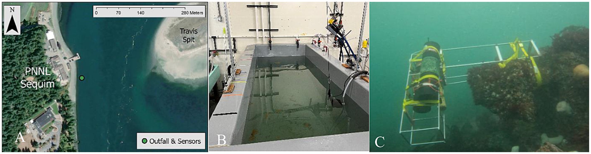
Figure 1. (A) Map of Sequim Bay channel and PNNL-Sequim. (B) Laboratory mesocosm used for both the sensor experiment and for the field experiment. (C) Deployment of YSI EXO2 pH sensor 15–20 cm from outfall pipes in the Sequim Bay channel.

Sequim Bay is a fjord-like tidally influenced semi-enclosed basin in the Pacific Northwest with a single narrow inlet at the northernmost point of the bay (Figure 1A). It has minimal freshwater influence and flushes at an approximate rate of once every 10 days (Khangaonkar et al., 2024). Tidal exchange in Sequim Bay averages ~2.5 m but can increase to more than 3 m during peak spring tides that result in tidal currents that can reach 2 m s⁻¹. Temperature and salinity in the Bay vary annually, and range between 29 and 32 PSU and 6–12 °C, respectively. Values for pH_NBS generally range from 7.6 to 8.3, depending on time of year and tidal conditions (Jones et al., 2025).

The mixing and dilution controls relating to alkalinity enhancement have been previously modeled in Sequim Bay (Khangaonkar et al., 2024). Sequim Bay is a unique location for testing point source release OAE due to its narrow inlet and high tidal currents that can potentially act to spread an alkaline plume over a large surface area, thereby increasing contact with the atmosphere. However, these rapid currents do not guarantee any confinement of elevated alkaline water at the surface, which poses challenges for determining the timing and location of an ideal release point.

2.2 Mesocosm sensors experiment

We conducted a mesocosm experiment to assess the performance of five commercially available pH sensors (Sunburst iSAMI, Seabird HydroCAT, Idronaut OS315, Yellow Springs Instruments (YSI) EXO2, and YSI ProDSS) and two commercially available pCO₂ sensors (Turner C-Sense and Batelle MAPCO₂/ASVCO₂) for monitoring alkalinity releases in coastal marine waters (Table 1). PNNL’s policy prohibits endorsement of commercial products; therefore, sensor manufacturers will not be explicitly linked to a specific sensor-measured data set in the mesocosm experiment. The sensors in the mesocosm experiment will be referred to as Sensors 1–5 from this point forward (Table 1). A 4000 L mesocosm tank was filled with raw Sequim Bay seawater and mixed continuously by two submersible bilge pumps placed in the tank on opposite ends (Figure 1B). All sensors were placed in the tank prior to the atmospheric pre-equilibration period and located in the same area within the tank. Atmospheric pre-equilibration of Sequim Bay seawater in the tank lasted 5 days before starting the experiment, allowing the sensors’ response to tank water to stabilize. Alkalinity (9.03 L of 0.5 M NaOH) was then added to the tank as a single dose, which was monitored for 28 days, until it reached near atmospheric equilibration in terms of pCO₂ values. After the 28 day, the sensors were removed and all data were exported for analysis.

Table 1

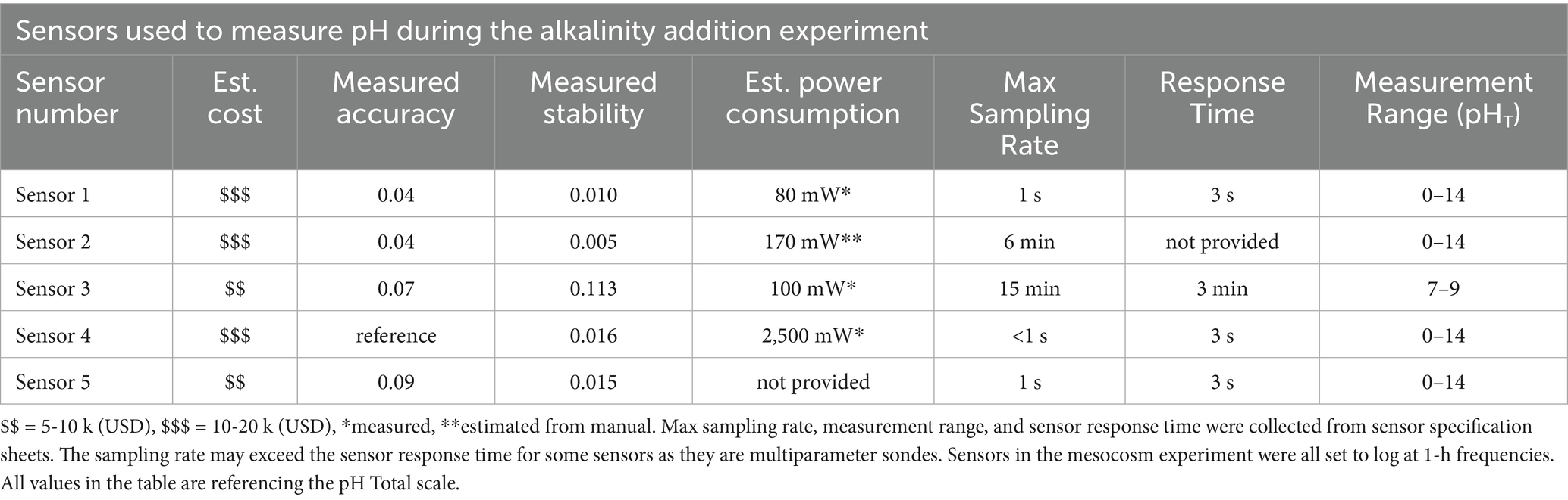
Table 1. Sensors used in the mesocosm experiment, including their estimated cost, relative accuracy based on mesocosm measurements (based on differences from Sensor 4, which was used as the reference), stability based on variance in hourly mesocosm measurements during the end of the experiment when values were most stable, and estimated power consumption.

All pH sensors across all experiments were calibrated to manufacturer specifications before and after deployment. pH Sensor 4 was calibrated with Tris buffer solution, in artificial seawater of salinity 35 [acquired from the Scripps Institution of Oceanography (La Jolla, CA, United States)], per manufacturer recommendations and measured pH on the total scale (pH_T). Sensor 3 was factory calibrated and measured pH on the total scale. All other pH sensors, measuring pH on the NBS scale (pH_NBS), were calibrated using a three-point calibration with National Institute of Standards and Technology (NIST) low ionic strength buffers at pH 4, 7, and 10. Pre and post-calibration values were compared to assess drift in sensor calibrations over the course of the experiment. All pH sensors were set to log at hourly intervals for the mesocosm experiment, with the exception of a hand-held sensor, which we used to measure pH twice daily during weekdays. Additionally, all pH sensor data not measured in pH_T were converted to the total scale following methods outlined by the seacarb R package (Gattuso et al., 2024) by first converting to seawater scale (SWS), then converting to total scale, and will be presented throughout the manuscript as pH_T, unless otherwise stated. One pCO₂ sensor had a continuous gas reference and did not require calibration, while the other sensors’ response was calibrated against a 411 ppm CO₂ reference gas standard prior to the experiment. The pCO₂ sensors were set to log at 3-h intervals during the mesocosm experiment.

To provide a ground truth for pH measurements, discrete samples for DIC and TA were collected daily in 250 mL glass bottles from the mesocosm tank, referencing methods from Dickson et al., 2007. Samples were preserved with 100 μL of HgCl₂ and analyzed via an Apollo SciTech Total Alkalinity Titrator (AS-ALK3) and Dissolved Inorganic Carbon Analyzer (AS-C6L), referenced against certified reference materials (CRMs). CRMs were run before and after TA and DIC sample analysis, resulting in a precision of ± 1 μmol kg⁻¹ for both parameters. pH_T was then calculated from the DIC and TA samples using the seacarb R package (Gattuso et al., 2024) referencing K1 and K2 dissociation constants from Lueker et al., 2000. The bisulfate dissociation constant from Dickson (1990) and total boron from Uppström (1974) were also used in the pH_T calculations.

2.3 Field test: Sequim Bay release

To test if alkalinity additions could be detected under real-world conditions and distinguished from natural variability, we conducted an alkalinity release from the PNNL-Sequim wastewater treatment facility’s outfall into Sequim Bay on February 7, 2025 (Figures 1A,C). (In this context, we use the term “test” deliberately: test deployments assess a single component or mechanism that is part of a larger technology or technical system, as here we test the capability of a particular sensor deployment configuration to detect discharge. A field trial, by contrast, is a rigorous performance evaluation of a well-established and previously demonstrated technology or technical system. A field trial would comprise a much longer and larger study across a series of discharges than was conducted by this study.) The same tank used in the mesocosm experiment was filled and maintained at a constant level with flowing raw seawater that was dosed with 0.5 M NaOH via a peristaltic pump at a rate that could maintain a pH_NBS ≤ 9.0 (as listed in NPDES permits). The outlet of the tank was plumbed into a wastewater treatment system where the pH was monitored and confirmed not to exceed a pH_NBS of approximately 9 (~8.9 pH_T) to maintain compliance with wastewater treatment facility discharge permits. The wastewater treatment system consisted of four cells that were sequentially filled with the effluent from the mesocosm experimental tank that connected to an outfall pipe in Sequim Bay. A total volume of 381 L (251 mol) of NaOH was diluted with ~180,000 L of ambient seawater, which was released from the outfall in four pulses, each separated by an hour, for a total of 8 h. Average flow conditions characterized by a ~ 2.5 m tidal exchange were observed during the release period, which allowed for a representative assessment of detection limits in this region.

We monitored the response in Sequim Bay to our pilot alkalinity release using a YSI EXO2 Sonde pH sensor attached directly to the outfall approximately 15–20 cm from the pipes (Figure 1C). The sensor was calibrated before and after deployment to the manufacturer’s recommendations, via the same methods listed in Section 2.2 for a three-point calibration, to account for drift and verify accuracy. The EXO sensor was installed 3 days before the release and recovered 9 days after the release. These data and a complete description of the field test methods are described by Savoie et al., 2025.

2.4 Idealized modeling experiments

We developed a simplified model based on Sequim Bay to explore the capabilities of multiple sensors to inform MRV efforts in a relevant coastal environment. These model scenarios were designed to quantify the MRV capabilities of commercially available sensors by incorporating (a) sensor performance metrics from the mesocosm experiment (Section 2.2) and (b) a similar-scale alkalinity release to the field test (Section 2.3). Averaged model outputs over a region of a detectable plume area were compared to model outputs sampled at discrete locations within said plume, mimicking the deployment of commercial sensors. This analysis provided a framework for assessing sensor capabilities to capture dilution and advection of an alkalinity release in a simplified channel that mirrors our field test environment.

The idealized model was developed within the Regional Ocean Modeling System (ROMS) framework (Shchepetkin and McWilliams, 2005) based on the marine carbonate system characteristics that roughly correspond to average Sequim Bay conditions (Figure 2). The idealized domain was developed with sloping boundaries in the across-channel direction and a maximum depth of 40 m to generally represent this type of coastal environment (Figure 2). This model grid has an average horizontal spatial resolution of ~60 m, an open boundary at the northern end of the simplified domain, a diurnally varying wind equal to ± 2 m s⁻¹ in the across-channel direction and ± 0.5 m s⁻¹ in the along-channel direction, and a regular tidal exchange of 3.5 m that is representative of regional tidal dynamics. Model outputs were saved every 2 h, and the barotropic time step was set to 20 s. Biogeochemical processes in this model are simplified and essentially contain only variables necessary for marine carbonate chemistry (i.e., model state variables include carbonate (CO₃²⁻), bicarbonate (HCO₃⁻), and total alkalinity (TA)). Total alkalinity is represented as carbonate alkalinity (computed as the sum of CO₃²⁻ and HCO₃⁻) and is permitted to equilibrate with a constant atmospheric CO₂ concentration of 422.5 ppm according to a standard ROMS subroutine (Fennel et al., 2008).

Figure 2

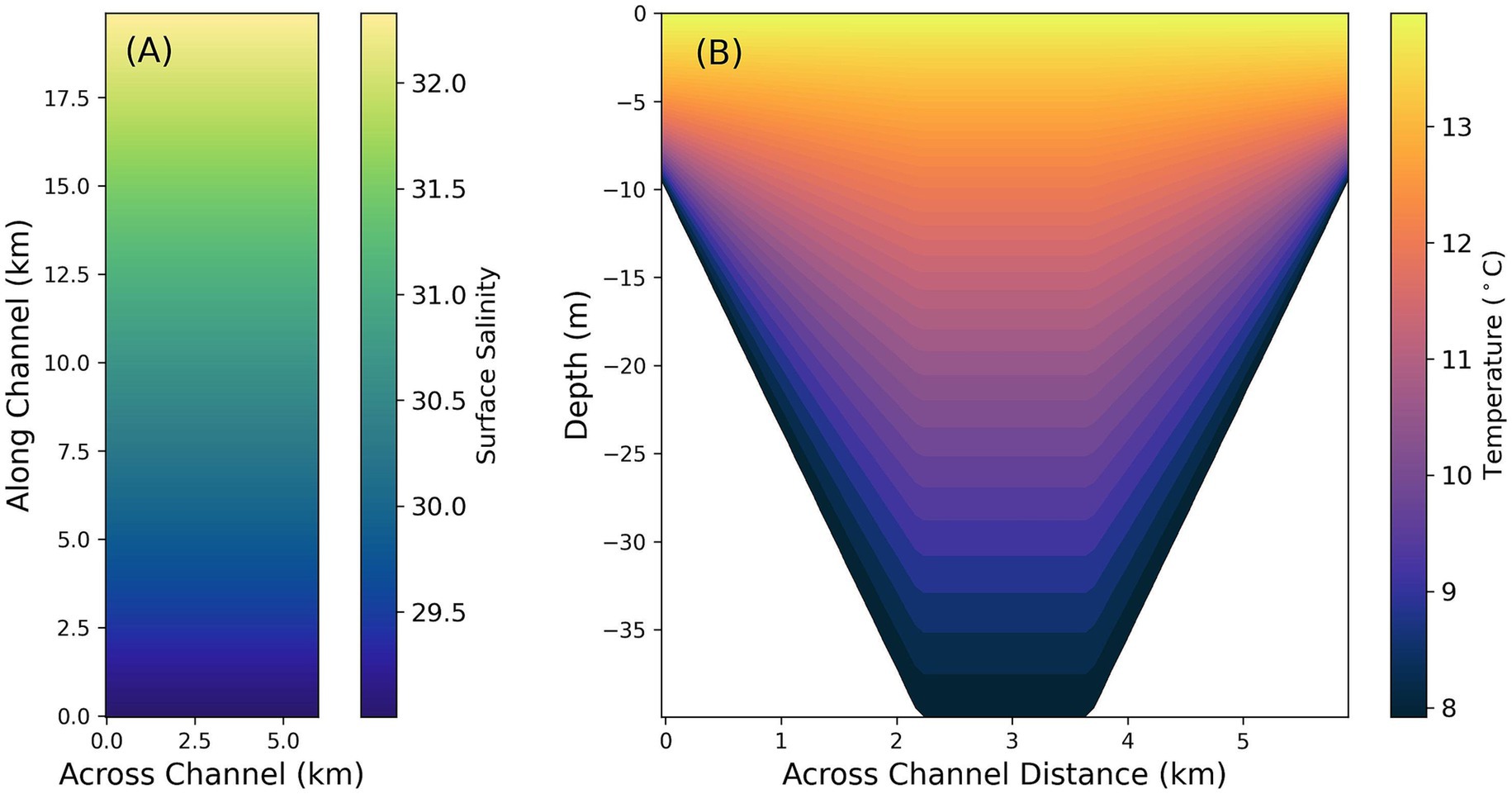
Figure 2. Sequim Bay, WA, idealized model domain with sloping walls and a maximum depth of 40 meters. (A) Plan view of surface salinity, constant with depth. (B) Along channel slice of model temperature.

The model was initialized from rest with a latitudinal salinity gradient and a vertical temperature gradient representative of average Sequim Bay conditions (29–32 PSU and 6–12 °C, respectively, Figure 2). Vertically varying biogeochemical values (higher at the surface, lower at the bottom) were applied throughout the domain at the initial time step (DIC = 2,110–2,350 μmol kg⁻¹, HCO₃⁻, = 1800–2000 μmol kg⁻¹, CO₃²⁻ = 158–176 μmol kg⁻¹, TA = 2,250 μmol kg⁻¹). These initial conditions were mirrored by the same constant open boundary conditions throughout the simulation. Two baseline simulations, with and without tidal exchanges, were first conducted over a period of 31 days to quantify the influence of open boundary changes on DIC and TA (S = 32, T = 9 °C). The closed boundary baseline experiment (‘Baseline Closed’, Table 2), while unrealistic in a marine system, essentially provides an upper limit on the capabilities of sensors to track changes to DIC and TA in a given domain and demonstrates the impact of natural variability in this region. Because the ‘Baseline Open’ experiment added no alkalinity, all changes to inorganic carbon in the model domain can be attributed to exchange processes with the open boundary (constant average DIC of 2,233 μmol kg⁻¹).

Table 2

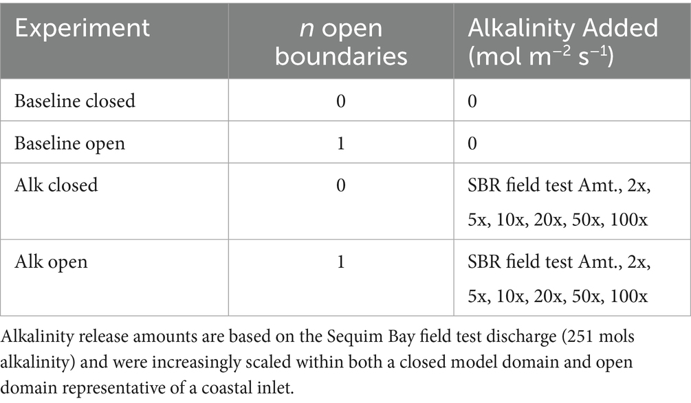
Table 2. Model experimental scenarios and descriptions.

Several modeling experiments were also conducted that increased alkalinity in a manner designed to simulate the addition of alkalinity in the SBR field test and explore the range of sensor sensitivities to increased fluxes. A surface flux of carbonate (CO₃²⁻) was injected into the center grid cell of the model domain over a period of 8 h, equaling the total applied in the SBR field test (1x, Table 2) for both a model domain with closed boundaries (‘Alk Closed’) and one with a single open boundary (‘Alk Open’). Additional alkalinity scenarios for the open and closed modeling domains were also conducted, where alkalinity was increased between two (2x) and one hundred times (100x) the amount of the SBR field test (251 mols of Alkalinity). While the closed boundary simulations are an unrealistic scenario for a marine system, they still present an opportunity to explore a hypothetical maximum limit on the ability of sensors to detect changes in the marine carbonate system that would be otherwise advected away or flushed through tidal mixing and currents. Values of pH_T were computed using PyCO₂SYS (Humphreys et al., 2025) to represent the sampling capabilities of multiple sensors for a plume in the idealized domain. Sampling bias was calculated by first taking the difference in mean pH_T (converted to [H+]) between alkalinity addition and baseline simulations, calculated for a specified number of stations (ranging from 3 to 100) and all available model cells. However, the average difference in modeled pH_T between the baseline simulation and an alkalinity addition was spatially limited to only include model cells where the pH_T change would be detectable at any point throughout the course of the simulation (Δ pH_T ≥ 0.01). Therefore, this bias calculation is constrained to only include areas of potentially detectable signals, which will likely remain uncertain prior to real-world alkalinity additions. After calculating the spatially limited differences between sampled cells and modeled cells versus a baseline (ΔSample and ΔModel), we calculated the percentage difference between ΔSample and ΔModel to determine the proportion of the pH_T signal that was capable of being captured by the sampling regime. Underestimates and overestimates of the captured signal are presented as negative and positive percentages, respectively. The positions of selected sampling points were randomly chosen in this subset of the model domain without replacement 10,000 times to more thoroughly evaluate possible surface sampling outcomes, with average changes and their associated standard errors computed for each sensor/alkalinity addition combination.

3 Results

3.1 Case study: commercial sensor evaluation and mesocosm tests

We first compare the specifications of 11 different commercially available pH sensors and eight pCO₂ sensors (Table 3), focusing on technologies that can be relatively easily deployed in coastal systems. The pH sensors described encompass a wide range of manufacturer-reported accuracies and can be broken down broadly into two categories: ion-selective electrode (ISE)-based sensors, spanning accuracies from 0.01–0.2 pH (NBS scale), and colorimetric/spectrophotometric sensors with accuracies of ≤ 0.01 pH (total scale). We observed general correspondence between accuracy and estimated cost, where sensors with lower accuracy were generally less expensive, although we note that estimated costs often included platforms (e.g., sondes, external batteries) as opposed to just the pH probe itself. All pCO₂ sensors included in Table 3 use the same measurement principle for quantifying gaseous pCO₂ (infrared (IR) absorption). However, they vary in terms of how CO₂ gas is extracted from water (e.g., gas permeable membranes vs. active equilibration) and how frequently calibrations are performed (e.g., prior to deployment vs. onboard span gas used to calibrate before each measurement). Similar to pH sensors, differences in cost often relate to the equipment necessary for proper operation of the sensor, including internal calibration capabilities and pumped heads for membrane-based sensors. On average, pCO₂ sensors cost more and have a wider range of accuracy compared to pH sensors.

Table 3

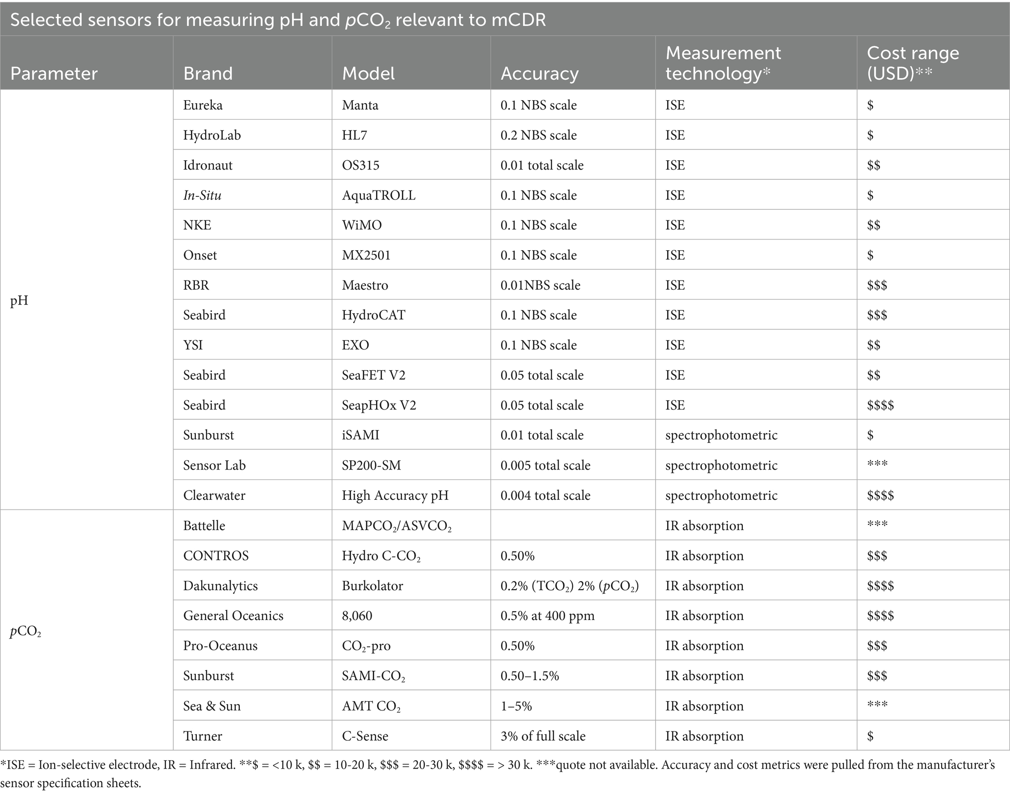
Table 3. Summary of commercially available in-situ sensors for monitoring mCDR applications in coastal marine systems.

We conducted a mesocosm alkalinity addition experiment to directly compare the performance of pH and pCO₂ sensors available for our specific application. To do this, we deployed a subset of the sensors (Table 3), including five pH sensors capable of being deployed in-situ in coastal waters and two pCO₂ sensors, representing a range of costs (Table 1). All sensors detected similar responses to the alkalinity addition and subsequent re-equilibration period over the course of the 28-day experiment, but some performed better than others (Figure 3). The initial spike in pH_T was detected by all sensors except Sensor 5, which had a delayed and decreased detection of the maximum extent, at least partially explained by a slower sampling rate relative to the other sensors (Figure 3A; Table 1). Sensors 3 and 5 had the greatest variability in pH_T during the least variable period, finding a change of roughly 0.07 and 0.09 pH_T, respectively. Additionally, Sensor 3 showed the most variability during the experiment (Figure 3A). The pCO₂ sensors had similar performance, with an average offset of 36 ppm (12% of benchtop sensor value) between the two sensors throughout the experiment. Offsets were the lowest immediately after alkalinity addition and increased as the experiment progressed (Figure 3B). The differences in pCO₂ values between the two pCO₂ sensors is likely due to autocalibration protocols unique to one sensor and the limited flow across the membrane of the other sensor, which would slow equilibration and result in consistently lower pCO₂ values, as was observed. To understand the deviation between each sensor and our reference sensor (Sensor 4, Table 1) during the experiment, we calculated point-by-point differences (Figure 3C). With the exception of one point for Sensor 5 showing a difference of > 1 pH_T during the period of largest change (e.g., the alkalinity addition), all sensors generally clustered near a difference of 0 with no clear temporal trends. We also plotted the linear relationship between pH_T measured by Sensor 4 and pH_T calculated using seacarb and TA and DIC samples measured in the lab (Figure 3D). We observed strong linearity and clustering around the 1:1 line, with an R² of 0.982 and an RMSE of 0.037 (or <1% of pH_T = 9).

Figure 3

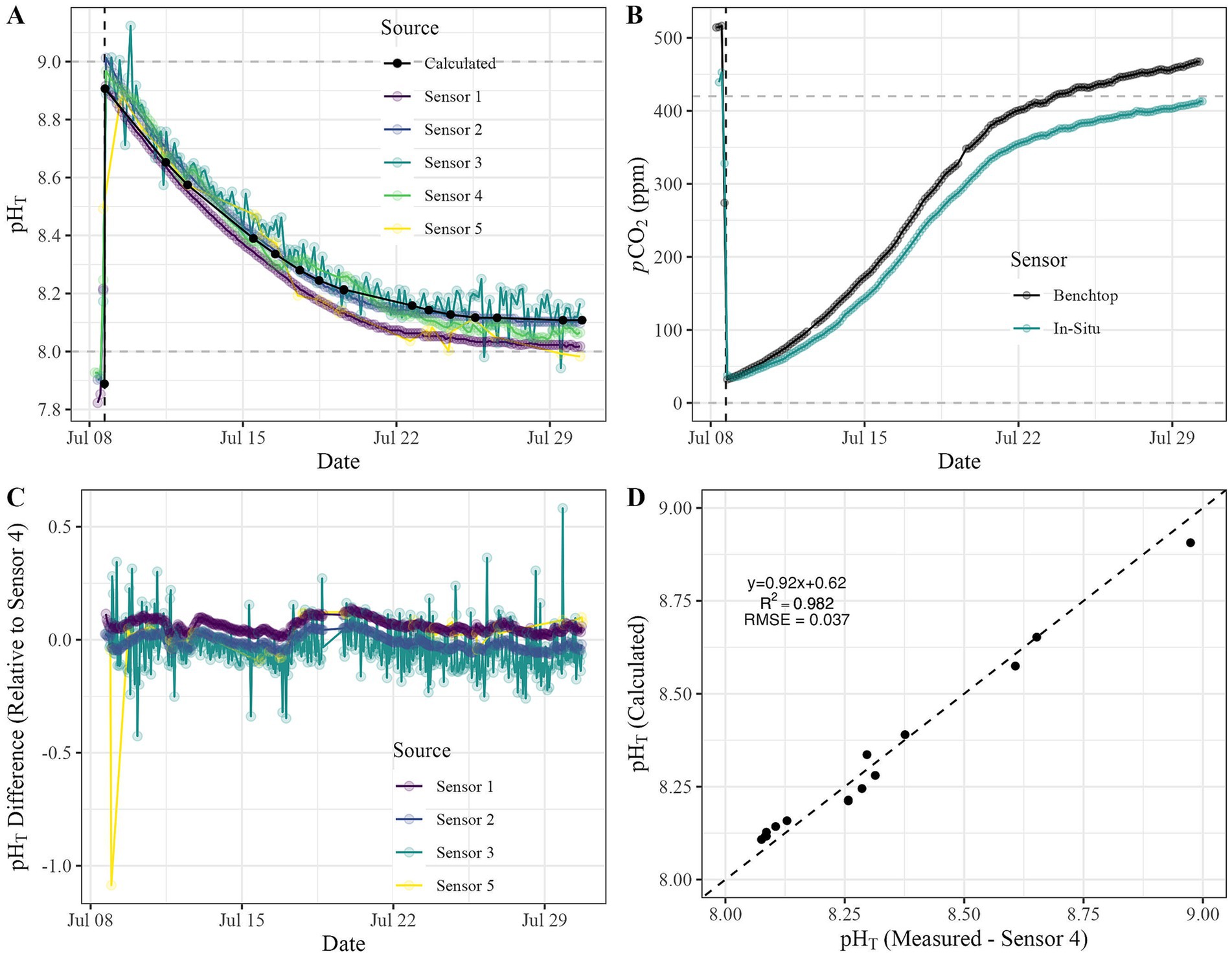
Figure 3. Time series for (A) pH_T (calculated pH values presented as black dots) and (B) pCO₂ measured during a 28-day alkalinity addition experiment conducted in the mesocosm tank shown in Figure 1. (C) We assessed the variance of each sensor relative to the reference pH sensor (Sensor 4) and (D) the relationship between pH_T. measured by Sensor 4 and pH_T calculated using TA and DIC laboratory measurements. The dashed black line represents a 1:1 relationship, and in-plot statistics present goodness-of-fit (R² of 0.982) and root-mean-square error (RMSE of 0.037).

We estimated sensor accuracy and resolution based on data in Figure 3, Table 1. We selected one sensor (Sensor 4) to be our reference sensor for calculating measured accuracy as it had the highest manufacturer-listed accuracy (0.01 pH_T), showed lower variability during the experiment, and had a dedicated reference probe (stable electrical potential to which the measuring electrode was compared). Estimated accuracies (relative to pH measured by Sensor 4) based on the measurements we collected in our mesocosm experiment were within the ranges reported by manufacturers (Table 3) and match the pattern that cost generally correlates with accuracy (e.g., lower cost equates to lower accuracy, Table 1). We observed almost two orders of magnitude in the range of our estimated sensor resolutions based on our datasets (Table 1).

To assess energy consumption under an OAE scenario, power consumption was measured for a subset of sensors used in the mesocosm experiment, also shown in Table 1. We report either values that we directly measured during sensor operations or estimates based on manufacturer-reported power consumption values when we could not directly measure power consumption without compromising the sensor. It should also be noted that no power-saving features, such as sleep modes or intermittent sampling strategies, were employed during this experiment. Power consumption (power use per day) varied between sensors by more than an order of magnitude, ranging from less than 100 mW to more than 2,000 mW (Table 1). While sensor energy consumption is likely minuscule compared to that of a given mCDR technology, there are both practical logistical considerations (e.g., time frame of deployment) and carbon accounting considerations (e.g., if a very large sensor network is required). Energy consumption is a particularly important consideration during remote and/or long-term deployments, where local offshore power sources, particularly tidal and solar, may be a primary limitation of sensor deployment length.

To understand how these differences in accuracy between sensors relate to estimates of marine carbonate chemistry, we conducted a sensitivity analysis where we set all parameters to assumed defaults (temperature = 25 °C, salinity = 35 PSU, pCO₂ = 420 ppm, pH_T = 8.0) and then manipulated either pH or pCO₂ values to replicate differences in accuracy represented across the sensors summarized in Table 1. For pH_T, we looked at accuracies ranging from 0.01 to 0.2 (Figure 4A). For all defaults, seacarb calculates an alkalinity of 2,145 μmol kg⁻¹. Using a pH_T sensor accuracy of ± 0.01, estimated alkalinity values had a range of 57 μmol kg⁻¹, with a maximum difference of 1.4% (percentage of the maximum difference from the default value of 2,145 μmol kg⁻¹). However, for the most common pH_T resolution (± 0.1), we observed a much larger range (1,107 μmol kg⁻¹), equivalent to a maximum difference of 29.4%. For the lowest accuracy represented in Table 3 (0.2) for a pH_T sensor, we observed a range of 2,383 μmol kg⁻¹, equivalent to a maximum difference of 71.2% (Figure 4A).

Figure 4

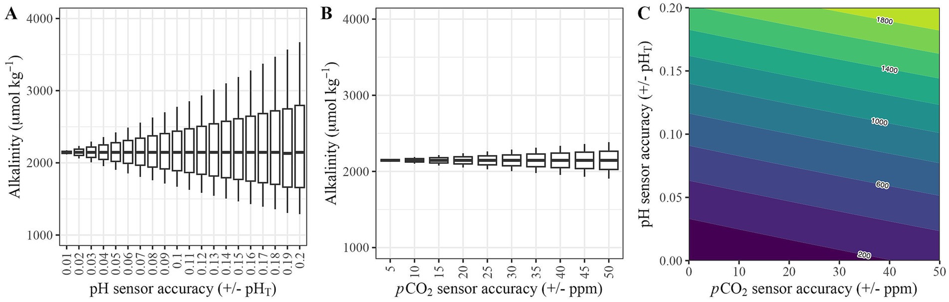
Figure 4. The relationships between sensor accuracy and alkalinity predicted by the seacarb R package for the accuracy ranges presented in Table 1 for (A) pH sensors, and (B) pCO₂ sensors were assessed. The range of sensor accuracies are presented in Table 1. Additionally (C) an error-space diagram to understand the combination of uncertainty in estimates of alkalinity for pH and pCO₂ sensors. The x-axis and y-axis are the ranges of accuracy presented in (A,B), and the contours represent the associated error (uncertainty presented as μmol kg⁻¹) of alkalinity estimates based on combinations of pCO₂ and pH sensor accuracies.

We conducted an equivalent sensitivity analysis where pH_T was held stable at 8.0, but pCO₂ values were manipulated from 0 to ± 20 ppm (approximately 5% of baseline pCO₂) at 2 ppm intervals (Figure 4B). Using a pCO₂ sensor accuracy of 2 ppm (~0.5% at 420 ppm), estimated alkalinity values had a range of 10 μmol kg⁻¹, with a maximum difference of 0.2%. The lowest accuracy sensor in Table 3 (± 5%) gave a range of 186 μmol kg⁻¹, with a maximum difference of 4.4%. Ultimately, there is better internal consistency when calculating the marine carbonate system using pCO₂ compared to pH_T in this analysis. To understand the combined impacts of the accuracy of pH_T and pCO₂ sensors on TA estimates, we constructed an error-space diagram (Figure 4C). Consistent with Figures 4A,B, the error-space diagram demonstrates that the accuracy of the pH sensor is considerably more important for reducing uncertainty in alkalinity estimates than the accuracy of the pCO₂ sensor.

3.2 Case study: SBR field test

Only a handful of OAE field trials have been conducted to date, turning a focus toward answering critical monitoring, reporting, and verification questions. Here, a proof-of-concept test was conducted to determine if in-situ pH sensors could detect a signal for an alkalinity release from an outfall into a tidally influenced channel in Sequim Bay, WA. Initial results from a YSI EXO2 pH sensor placed directly at the outfall indicate that, at close proximities, sensors could detect a signal as all four pulsed releases were detected outside of the range of normal observed variability (Figures 5A,B). However, the pH_T signals detected (15–20 cm from the outfall) were significantly diluted (~7.8–8.25) compared to the pH_T measured at the end member of the wastewater treatment system (~8.9).

Figure 5

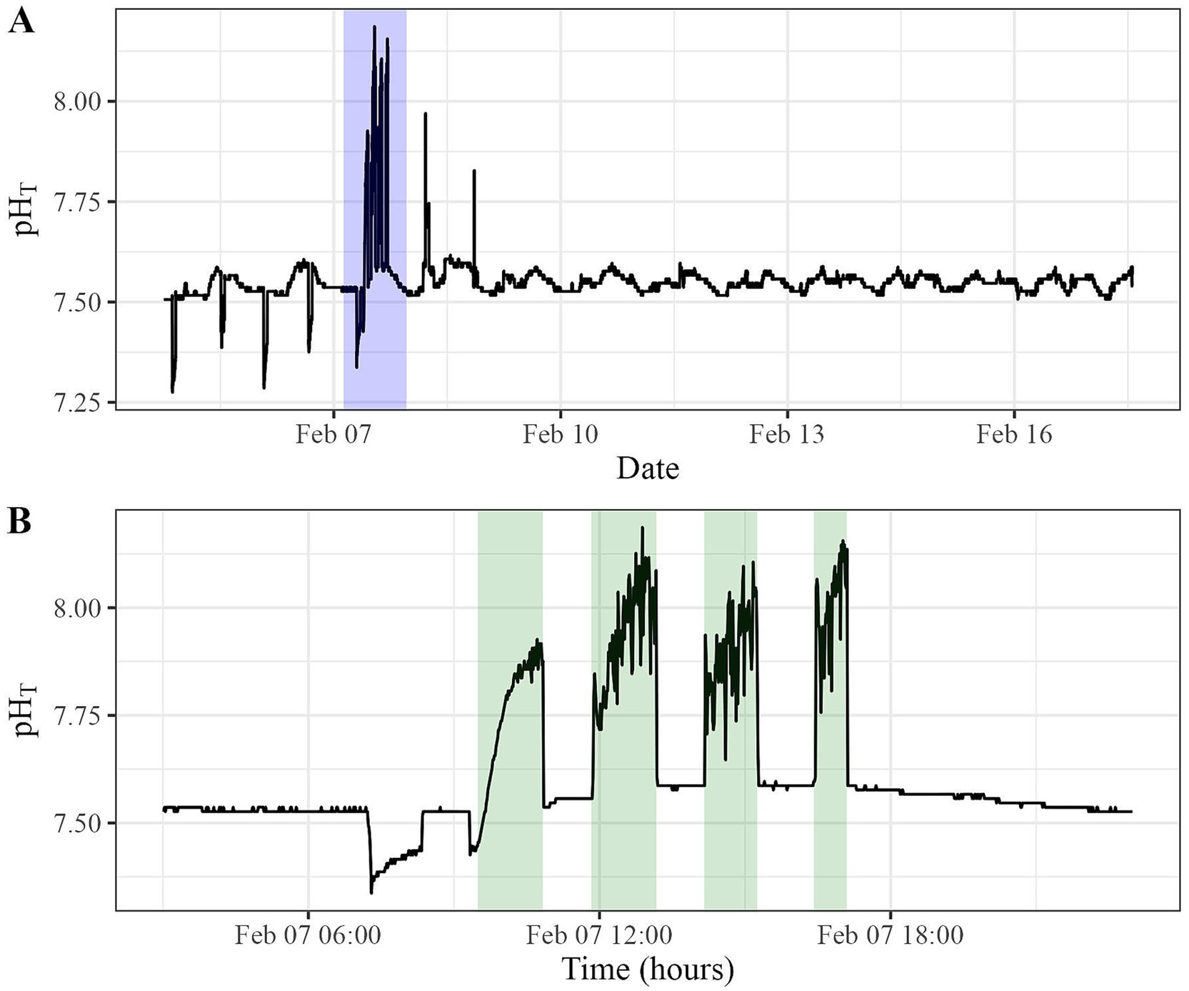
Figure 5. (A) YSI EXO2 Sonde pH time series recorded during an alkalinity release from a wastewater treatment outfall in a tidally influenced channel. (B) Four pulses were detected during the release over 8 h, each separated by 1 h.

The baseline pH_T conditions prior to the release were between 7.5 and 7.6. Each pH_T pulse released from the wastewater treatment system was detected between 7.8 and 8.3 (Figure 5). The variability observed along the baseline prior to and during the first step is likely due to tidal influence, followed by unmixed freshwater also exiting the cell during the first release (Figure 5, Panel B). Following the first release, the pH_T signal was observed to drop sharply off after each release, returning near the baseline almost immediately each time. The gradual slope, showing an increase in alkalinity during each of the four releases, is likely because the drainage of the wastewater cells was faster than the dilution of the system around the sensors (Figure 5). These sensors performed adequately from a permit compliance standpoint, verifying that we did not exceed the pH_T ~ 8.9 threshold of our NPDES permit (converted from NPDES permit threshold of pH_NBS 9.0). However, the sensor performance indicates that detectability beyond the outfall for carbon accounting purposes is a much larger challenge. More details about this field test can be found in Savoie et al., 2025.

3.3 Case study: modeling

A surface flux of alkalinity in the center grid cell of the idealized model domain was applied to simulate the dilution and detectability of an alkaline plume under hydrodynamic and tidal conditions representative of Sequim Bay. At the release level of the Sequim Bay field test, there were extremely low to no levels of detectable change, depending on the use of a 0.01 or 0.001 pH_T threshold. Therefore, the model results for the 100x experiment are plotted to show a larger areal extent of pH_T changes that would have a greater likelihood of detection (Figure 6). Results from the two baseline experiments demonstrate that ~10–11% of the apparent signal at the surface of the domain cannot be captured by pH_T sensors with an accuracy of 0.01 units [referencing Sensor 4 manufacturer reported accuracy of 0.01 pH_T (Table 1)] with an open boundary after a period of 1 week due to the effects of vertical and lateral mixing. Subsurface plume mixing and advection out of the inlet both contributed to continuous dilution, challenging the coherence of a signal corresponding to increased pH_T (Figure 6). When compared to the full volume of the idealized domain, tidal exchange irreversibly diluted this signal after ~3 days, and this fraction of alkalinity-enhanced waters exiting the surface of the model domain steadily increased thereafter for the remainder of the simulation.

Figure 6

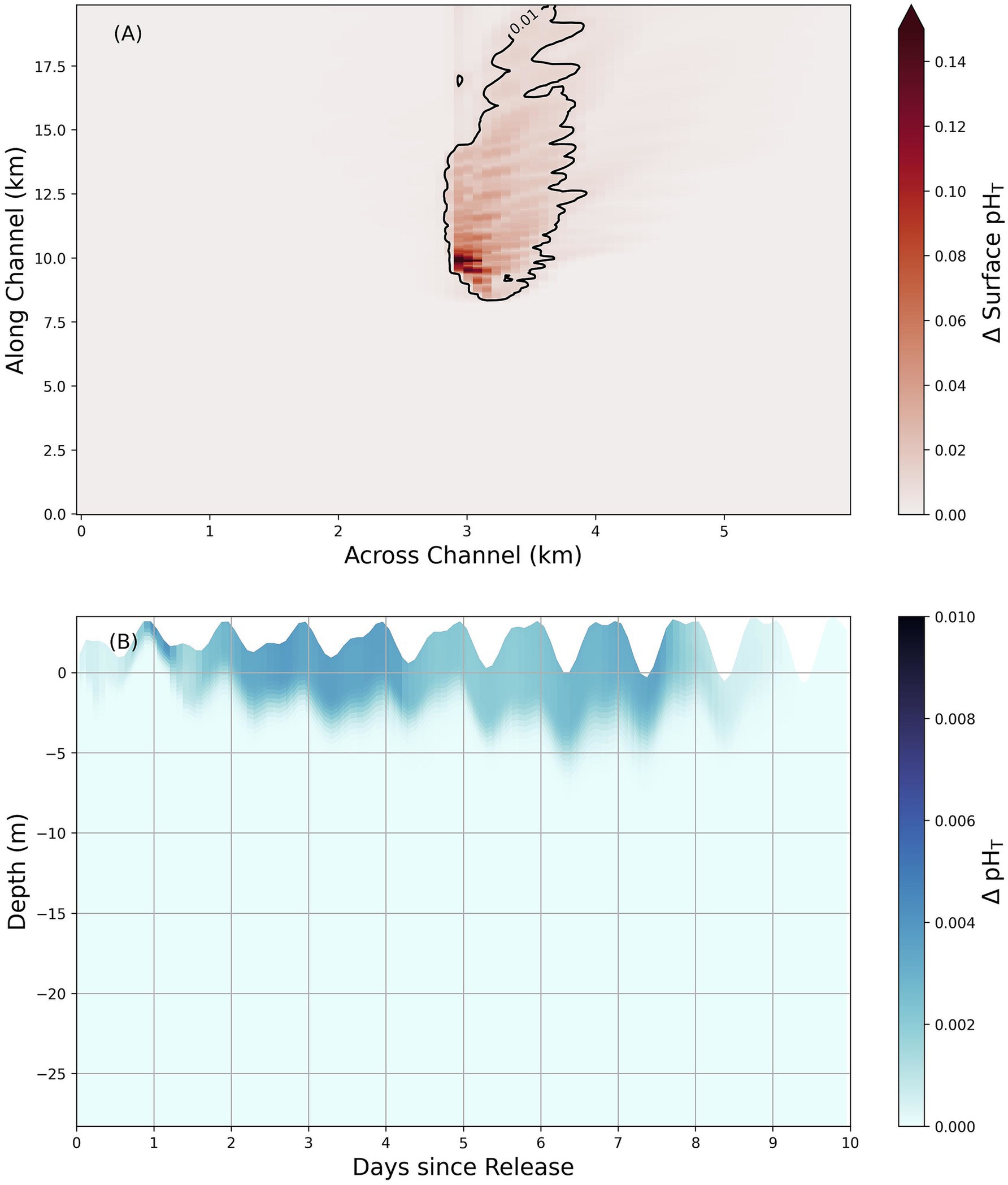
Figure 6. 100x model scenario from SBR field test showing the maximum spatiotemporal extent of changes to pH_T following an alkalinity release. Panel (A) shows surface pH_T changes in a Sequim Bay-like basin with an overlaid 0.01 contour while panel (B) shows the horizontally averaged pH_T changes at different depths (varying with the imposed tidal cycle) over the same domain for all cells that lie within the contour of 0.01 pH_T detectability shown in (A). Both panels show the changes in pH_T following a release that is 100 times the amount that was actually discharged (251 mols of alkalinity) into Sequim Bay over the same duration. Note that the color bars and scales differ between panels (A,B).

Changes to pH_T levels (calculated from modeling results using PyCO₂YS; Humphreys et al., 2025) show that the limits of detectable changes are confined to a small area near the alkalinity addition point in the center of the model domain, even at alkalinity release levels 100 times greater than the SBR field test (Figure 6A). For an alkalinity addition equal to the SBR field test (1x, Table 2), the maximum signal is undetectable at a 0.01 pH_T threshold for the area surrounding the deployment site over the first 10 days following the alkalinity addition, and only covers an area of approximately 0.11 km² if a 0.001 pH_T threshold is applied instead. As expected, this detectable range expands as the amount of added alkalinity increases: at 10 times the SBR field test, the maximum extent of pH_T covers an area equal to ~0.11 km², increasing further to 7.4 km² at 100 times the SBR field test for a 0.01 pH_T threshold. Even with a comprehensive sampling network of 75 sensors evenly spaced throughout the inlet at regular 1 km intervals, ~93% of the sampled stations would be unable to detect a signal in a scaled version of the SBR field test model experiment (100x) based on current precision levels of market-available pH_T sensors assessed during the mesocosm experiment (Tables 1, 2).

With an increasing number of sensors, we find that the uncertainty in capturing the change in the overall pH_T signal improves (decreased standard error bars), but consistently under-reports the true change in modeled pH_T (Figure 7). With a much larger release of alkalinity (100x), the number of sensors underestimates the true change in pH_T signal by approximately −35.9 ± 18.1% (−0.003 ± 0.002 pH_T) and −36.4 ± 0.5% (−0.003 ± 3.8E-5 pH_T) for the sparsest (3 sensors) and densest (100 sensors) observational configurations, respectively. This inability to fully capture the average change in surface pH_T is likely due to imperfect mixing of the change in DIC within the region where sampling occurs and where any signal is potentially detectable by sensors (≥ 0.01 pH_T). A fraction of the change to surface alkalinity that lies below the detection limit will also consequently be lost to monitoring efforts. At relatively small releases (1x, 2x), 5 sensors are adequate to fully sample the area that is affected by increased alkalinity changes within the specified detection limit (≥ 0.01 pH_T). At larger releases (50x, 100x), a release of 100 sampling sensors will only capture ~5–13% of the total surface pH_T change for an area where the detection limit will meet the specified threshold for a single time step in the model simulation (increasing to ~14–19% for a pH_T threshold of 0.001). Over time, alkalinity changes are mixed deeper in this idealized domain, where no air-sea equilibration can occur. This represents another limitation of capturing the total change in pH_T. Some percentage of this subducted alkalinity eventually is exchanged with the open boundary, which challenges even the most comprehensive surface monitoring network that could be deployed in a small coastal inlet. In model simulations with no open boundaries, the ability to detect the true signal with surface-only observation points slightly improves while the standard errors hardly differ (e.g., underestimated by 34.7 ± 0.4% at 100x the SBR release levels for 100 sensors). These findings are well-aligned with near-field plume modeling results that suggest the pH_T signal will rapidly dissipate within several meters of the outfall (Savoie et al., accepted), highlighting the need to integrate subsurface monitoring assets into mCDR and MRV applications.

Figure 7

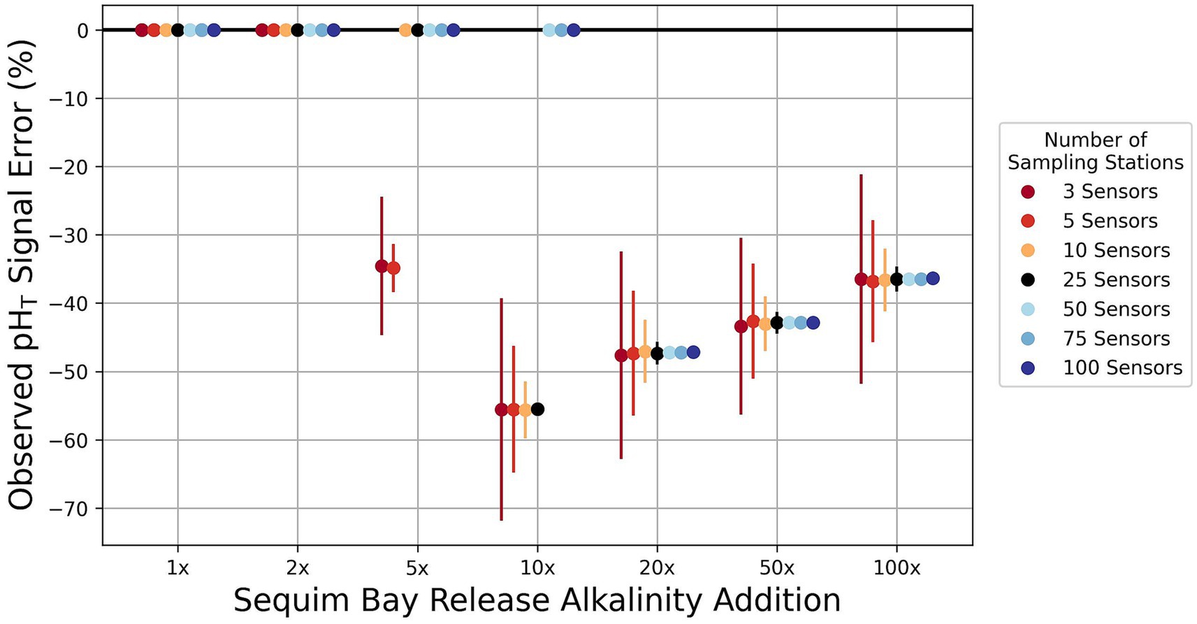
Figure 7. The magnitude of errors in the percentage of the pH signal captured using multiple stations compared to the model output in regions where a signal would be detectable. This percentage error varies based on the size of the alkalinity release. 1x is equal to the Sequim Bay field test release, 2x is two times that amount over the same time period (8 h), etc. The average difference between sampled and modeled surface pH_T changes are divided by underestimates (negative values) and overestimates (positive values). Standard errors of the percent of the signal captured by the number of sensors are displayed as error bars. Points for alkalinity additions that lie on the zero line perfectly capture the modeled signal because the number of stations is greater than the number of model cells where a detectable signal can occur. The averages and standard errors are computed from 10,000 sampled estimates.

4 Discussion

4.1 Monitoring: sensing

Accurate monitoring, reporting, and verification of mCDR applications are constrained by our ability to measure impacts at relevant spatial and temporal scales. This is a difficult task, particularly in coastal systems, where tidal, diurnal, and seasonal patterns all influence water chemistry. To better understand our monitoring limitations, sensors and models need to be assessed in these conditions.

Accurate monitoring of OAE is partially limited by the instruments available to measure parameters with suitable accuracy, which are currently benchtop instruments that require discrete samples with sufficient volume and careful sampling procedures to avoid atmospheric contamination. Alternatively, measurements can be collected to parameterize the marine carbonate system and then estimate all other components, including TA and DIC, using popular packages like CO₂YS (Pierrot et al., 2021) or the seacarb R package (Gattuso et al., 2024). These algorithms require measurements for two of four components: pH, pCO₂, TA, and DIC. In-situ pH and pCO₂ sensors are the most established to date (Briggs et al., 2020; Briggs et al., 2017; Byrne et al., 2010; Shangguan et al., 2022; Shangguan et al., 2021), can measure at high temporal resolutions, and provide an alternative to the collection of discrete samples. While this approach allows for a large increase in the frequency of measurements that can be collected autonomously, it is also subject to propagation of errors from sensor accuracy, sensor calibrations, and uncertainty introduced by estimating marine carbonate chemistry conditions from these measurements (Miller et al., 2021b; Miller and Kelley, 2021a). Sensors will need to be carefully selected for a given environment with consideration given to maximum sampling rates, measurement range, and sensor response time. For OAE, accurate measurements of TA and DIC are a current limiting factor: both are required for accurate accounting of sequestered carbon, and they are spatiotemporally variable with limited reliable in-situ sensing solutions available for either (Briggs et al., 2017, 2020; Byrne et al., 2010; Shangguan et al., 2021).

A range of pCO₂ sensors of varying costs and accuracies are currently available (Briciu-Burghina et al., 2023), but the underlying detection method of each sensor has its own limitations (Clarke et al., 2017). This also includes the limitations associated with the skill and experience of sensor operators (McLaughlin et al., 2017). pCO₂ sensors typically cost more than pH sensors (Table 3), but there is better internal consistency in the marine carbonate system when using pCO₂. While pH is a comparatively cheap and simple measurement to collect with an in-situ sensor, it is challenging to capture high-quality samples in coastal systems (Gonski et al., 2024; Herrmann et al., 2020; Miller et al., 2018), where many early OAE deployments are likely to take place. Calibration is critical for pH sensors, and in environments with dynamic salinities, it can be challenging to consistently match the salinity of the sample being tested to the salinity of the calibration buffer (Dickson et al., 2007; Easley and Byrne, 2012; Martell-Bonet and Byrne, 2020). To combat this several methods have been developed to calibrate pH sensors in dynamic systems, including in-situ or field calibrations (Bresnahan et al., 2014; Gonski et al., 2024). Drift can also become an issue for pH sensors over time due to biofouling and degradation (Briciu-Burghina et al., 2023; Delauney et al., 2010; Martz et al., 2015), as well as instability issues arising from temperature fluctuations during the day (Shen et al., 2024). However, with the current state of technology, when done well, pH will be a critical parameter for monitoring OAE. A well-constrained pH measurement will be critical for accurate monitoring of mCDR efforts if pH and pCO₂ are chosen as primary measured marine carbonate system parameters. Our results show that the pH sensors’ estimated accuracy was better than the manufacturer’s reported accuracy for all except one sensor during the mesocosm trials (Table 1). This suggests that rigorous accuracy testing using redundant sensors and/or discrete samples by sensor users is one potential way to increase confidence in lower-cost sensor data. Our results also highlight that more error is induced when calculating other marine carbonate system parameters, specifically TA, when pH is poorly constrained compared to pCO₂ (Figures 4A,B).

Outside of error propagation, understanding the detection limits of in-situ sensors due to dilution will be critical for determining the number and appropriate spatial distribution of sensors during OAE monitoring efforts. The mesocosm study highlights sensor performance in a closed system, but the field test and model showcase how quickly dilution impacts detection capability in an open system. During the SBR field test, at a 15–20 cm spacing away from the outfall, a dilution from pH_T 8.9 (measured before release) to ~7.9–8.1 was observed (Figure 5). At the same level of release, with any further distance from the outfall, detecting a measurable signal would be challenging with current pH sensor capabilities (sampling rates and sensor response times). Additionally, the influence of tidal exchange during the release was average for Sequim Bay. Increased dilution effects during larger tidal exchanges will also decrease the likelihood of signal detection, even at close proximities. These environmental challenges highlight the complexity of working in dynamic (tidally influenced) areas. Importantly, we note that matching sensing capabilities/settings to the persistence of the perturbation being measured is important not just across space but also through time. Accurately capturing system responses to mCDR interventions, critical for effective MRV, depends on three separate time-scales aligning: (1) the sensor response time– how rapidly the sensor can complete a measurement, (2) the sensor measurement interval – how frequently measurements are collected, and (3) the persistence of the perturbation – how long is the measurable signal present in the volume sampled by the sensor. As an example of how these three time-scales interact, a sensor with a response time of 1 s can measure a perturbation lasting 2 min. However, if the sensor is set to measure at 5-min intervals (a common measurement frequency that provides temporal resolution while saving battery and memory), it is likely it will miss the peak of the event, and may miss the event entirely. To improve the chance of signal detection, consideration during sensor selection should be given to the timescale of sensor response time, measurement range, and sensor measurement frequency. Ultimately, sensor accuracy will be irrelevant if it is not deployed in the correct location and sampled at sufficient temporal resolution and response time to capture the system’s response.

Powering sensing efforts in marine environments can be complex, especially at scale. Energy consumption, more broadly for all parts of mCDR deployment efforts, should be evaluated, including tools for MRV. Whereas general power consumption information provided on manufacturer sensor specification sheets is typically based on ‘normal’ operating conditions. These are far less dynamic than coastal regions and ranges that may be experienced during OAE deployments. Energy consumption for the five sensors tested ranged from 80 to 2,500 mW, which would be easily supplied by most tidal or floating solar setups (Table 1). In 1 year, at the measured rates of consumption, the sensors tested would consume 0.7 to 21.9 kWh of energy if run continuously. For context, a tidal turbine, with a 1 m² cross-sectional area, placed in Washington State tidal hotspots (annual available energy ranging from 411 to 19,657 kWh m⁻²) would have the potential to generate 102.75 to 4914.25 kWh annually (calculated using a conservative estimate of turbine energy conversion efficiency of 25%) (Yang et al., 2021).

That is two orders of magnitude more power than the sensors’ max draw. To power sensors at 2500 mW, you would need almost 6,000 18,650-format lithium iron phosphate batteries a year. However, these power consumption estimates do not account for additional factors, including ancillary power needs (e.g., active anti-fouling solutions and/or pumped water or air), user-configured deployment configuration (e.g., sample averages and measurement frequencies), or variation in power production in response to dynamic environmental conditions. Our results suggest that sensor energy consumption is an important consideration but likely will not be a limiting factor for field trials. Instead, we suggest that further research is needed to determine appropriate power sources for scaled-offshore mCDR deployments.

4.2 Models informing monitoring

Due to the cost and complexity of high-resolution sampling, practitioners will have to rely on models (in tandem with sensors) to adequately monitor OAE application and impacts. Models have the potential to forecast changes to key marine carbonate system variables, inform the total potential for the scale of CO₂ removal, and assist in predicting long-term impacts on biogeochemical processes. Our results highlight the utility of relatively simple idealized models for designing measurement strategies and predicting changes in the marine carbonate system. The use of more complex numerical Observing System Simulation Experiments (e.g., Hoffman and Atlas, 2016) is common practice for designing large-scale open ocean sensor deployments (e.g., Gasparin et al., 2019; Valsala et al., 2021; Vecchi and Harrison, 2007) but is less commonly employed for nearshore coastal studies. Such experiments are critical for coastal environments, given the highly variable conditions in which OAE interventions might be deployed and the uncertainty of the spatiotemporal resolution and number of sensors needed for a given environment. Prior to deployments, such models can be used to determine the number of sensors or monitoring stations required to capture some percentage of the total signal, given the detection limit of a sensor. As shown in Figure 7, increasing the number of stations can substantially reduce the level of uncertainty among a sampled average, and this effect is greatest when smaller amounts of alkalinity are released. Consequently, reducing uncertainty in observed changes to pH or pCO₂ will also require more power for the sensors utilized. Additionally, models can be used to better determine where sensors should be deployed in order to increase the probability of success that an OAE signal can be effectively targeted and detected for a specified period of time.

Our results highlight how a comparatively simple model can be used as a MRV testing tool, informing field trials and deployments before they are conducted. Alkalinity added to the idealized model is rapidly diluted despite the domain starting at rest and applying a minimal wind. This emphasizes the narrow period over which changes can be detected and accurate accounting of the carbon budget through monitoring efforts can be carried out (Figure 6). The relatively brief window over which changes can be detected also holds true for a closed basin that has no tidal exchanges, demonstrating that the speed of dilution presents a substantial challenge for monitoring efforts. Some of this OAE signal is also lost to depth, meaning that a more complete accounting of the alkaline plume would also require an increased number of subsurface sensors that are not evaluated here (Figure 6B). Further, accurate detection of an OAE signal by surface pH_T sensors underestimated the total detectable change by ~35–55% on average across all model experiments, whenever the number of model cells experiencing a pH_T threshold > 0.01 exceeded the number of sensors released (Figure 7). The role of spatial variability within the region of detectable pH_T changes also acts to limit the accuracy of sensors in capturing the average change, even at high sampling densities (50–100 sensors). Point measurements in this framework are limited, and a residual bias may be reduced if the sensors were permitted to drift, rather than remain in fixed positions. However, such an adjustment naively implemented is also an inherently limited strategy. Selecting random locations within the region of detectable influence based on the approach taken in this work only slightly reduces the uncertainty of measurements without meaningfully affecting sampling bias (Figure 8). Optimizing sensor placement to accurately capture changes to pH_T and alkalinity in real-world field trials will face additional hurdles. Chief among these challenges are the uncertainties in simulated trajectories of an alkalinity plume which will limit the ability of more robust sensor placement approaches to accurately predict changes in pH_T and alkalinity. MRV efforts may be best supported by regular gridded sampling over an area where a plume is expected to reside for a period of time, through drones or other novel technologies like towed sensors or pH-sensing cables. More statistically robust sampling methods should also be investigated to be paired with novel sensing technologies. Selecting points with the highest gradient in concentration of alkalinity may over-represent expected changes, while k-means clustering type algorithms may more accurately represent average conditions over the lifetime of a deployment. A more thorough investigation of possible techniques in conjunction with field trials will likely help to identify additional promising sampling approaches that are beyond the scope of this paper. Altogether, these results highlight that high-resolution models are likely the best option to represent alkalinity plume dynamics in complex environments and will be a critical tool to help inform the optimal placement and distribution of in-situ sensors.

Figure 8

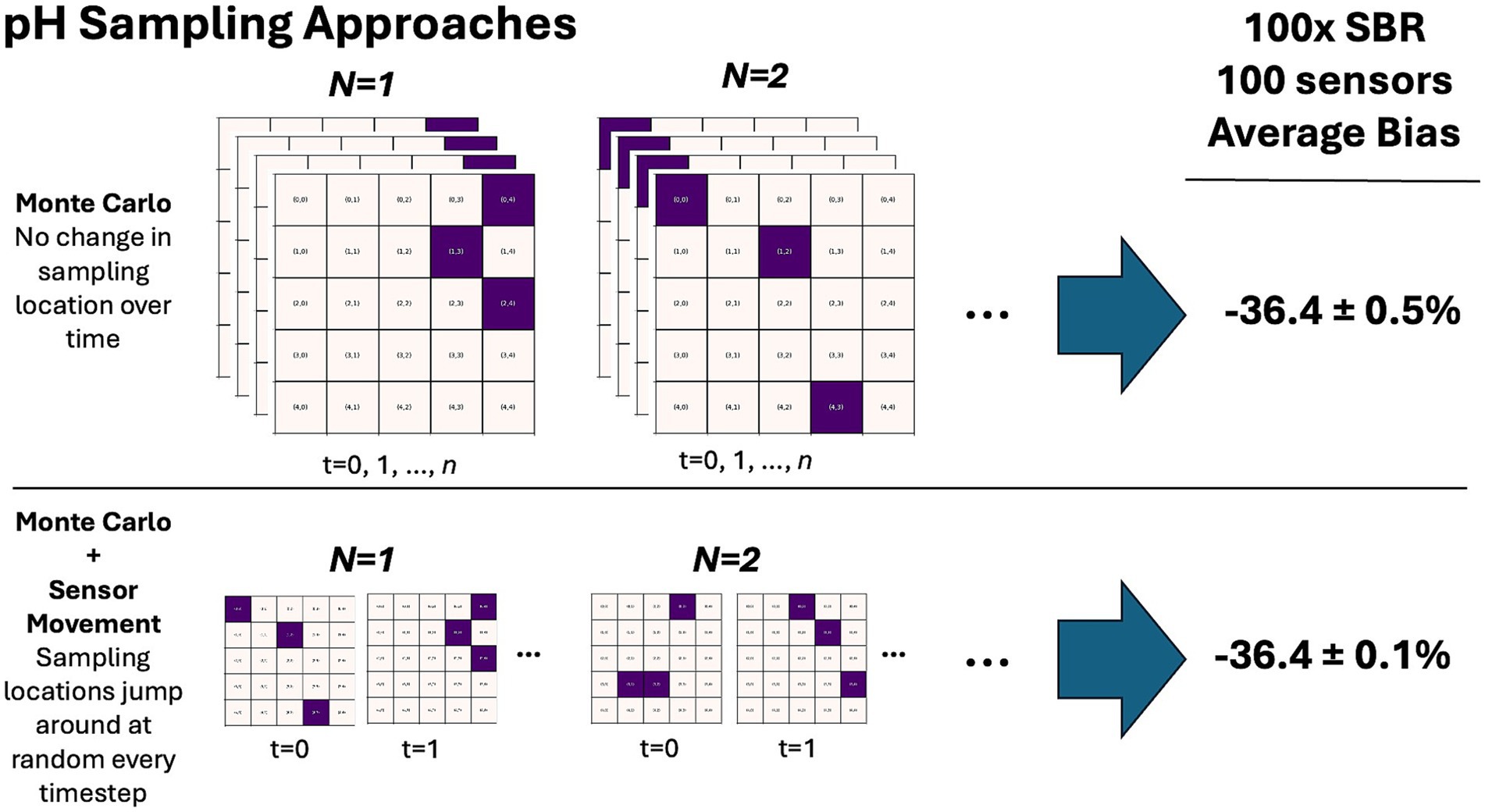
Figure 8. Comparison of synthetic sampling approaches characterized by the random placement of sensors within a detectable plume area. In the top row, a number of random points are selected for model sampling in a given Monte Carlo iteration. These points remain fixed over the duration of the sampling process, and the overall estimate of bias and associated standard error are equivalent to the 100x alkalinity release using 100 sensors shown in Figure 6. In the lower panel, these sampling locations are permitted to randomly adjust at each time step. Allowing the locations of the sampling points to move does not substantially lower the average bias but does reduce the associated standard error.

4.3 Key recommendations

4.3.1 Improvements: sensors and models

High-quality mCDR projects should strive to implement best practices that reduce uncertainty and minimize error in detecting and quantifying total rates of carbon removal. Making direct measurements of TA and pairing TA with DIC to calculate the rest of the marine carbonate system would reduce error propagation (Orr et al., 2018). However, TA and DIC are challenging to measure in-situ, creating important bottlenecks and limitations for the amount of data that could be collected, especially in cost-limited contexts. At least for now, autonomous, high-resolution pCO₂ and pH sensors are likely to form the backbone of mCDR MRV data collection. Reducing the costs of these sensors and improving their drift could support incremental improvements to the uncertainty of data collected by these sensors and cost-effective monitoring campaigns. Biofouling represents another key source of uncertainty not assessed in the short sensor deployment described here. Research is being conducted to determine how to combat biofouling, including using coatings and wipers, but only a handful are commercially available (Delauney et al., 2010).

In addition to the environmental challenges, sensor response time and maximum sampling frequencies may dictate or skew what perturbations can be captured through sensing alone. Sensor selection should be guided by the three time-scales described above (sensor response time, sensor measurement frequency, and persistence of perturbation). As an example, deploying less accurate sensors capable of finer temporal resolution alongside more accurate sensors with coarser sampling frequencies could provide opportunities to effectively interpolate higher-accuracy, sparser measurements based on the lower-accuracy, temporally resolved time-series.

While the accuracy of data collected is essential, sometimes even the most accurate sensors will struggle to detect a large signal against dynamic background variability. Within existing literature and frameworks, there has been a call for establishing and collecting baseline measurements prior to conducting mCDR activities (Boyd et al., 2023; Cross et al., 2023; Ho et al., 2023; Niffenegger et al., 2023). To adequately understand the chemical changes, biological response, and long-term impacts of OAE application, an understanding of the local marine carbonate system is crucial. Additionally, it has been noted that understanding the ‘additionality problem’, in relation to the extent that anthropogenic alkalinity alters the baseline or delivery of natural alkalinity, also needs to be addressed in monitoring efforts (Bach, 2024). Ultimately, monitoring practices long-term will need to be able to address both additionality and durability (Ho et al., 2023). Improvements to sensors would therefore benefit the development of readily available baseline data sets for OAE applications in environments of interest. In turn, this would advance the capabilities of sensors used to validate and inform models, quantify shifts outside ambient background variability, and support carbon markets. Historic environmental data can also be leveraged to support this effort, and improve the understanding of long-term trends.

Regardless of sensing method, direct observations will not be able to track 100% of changes induced from OAE (Ho et al., 2023), especially at large spatial scales. To adequately support these efforts, models will first need to accurately simulate key physical dynamics for extended periods (weeks to months) to capture equilibration timescales. Additionally, improvements in the representation of fine-scale dynamics and biogeochemical dynamics (e.g., secondary precipitation and potential modifications to air-sea fluxes) may be required, which can be very computationally demanding (Ward et al., 2025). These conditions should be explored further as real-world releases of mCDR efforts are likely to push many existing regional biogeochemical models outside the range of historically simulated model limits. More generally, expanding the user interface and accessibility will also be critical to the long-term development and support of these models for MRV efforts.

4.4 Clear MRV standards

Although mCDR research continues to advance, general guidelines are needed to structure current and future research to advance the field in tandem with sound science. Specific MRV guidelines will need to be developed in tandem to adequately support the development of the field. Some progress has recently been made clarifying suggested MRV practices related to specific technologies and carbon registries more generally (e.g., Agbo et al., 2024; Isometric, 2025; Myers et al., 2024). Scientists have also begun to compile best practices guides (e.g., Oschlies et al., 2023). Work to develop consensus standards among scientists and professionals is ongoing, and will need to be routinely assessed and updated as more sensors and models are developed, more field tests and trials are completed, and more regulations are enacted.

4.5 mCDR collaboration

Collaboration between mCDR monitoring campaigns is likely to be crucial to the success of each individual effort. This research could not have been completed without collaborating with scientists from various backgrounds and expertise. However, with the current lack of data sharing, it was challenging to collect sensor specifications and costing and compare results to similar mCDR studies. Previously, laboratory and sensor intercomparison projects (e.g., Bockmon and Dickson, 2015) have also identified analytical differences across different expert users, and this has been especially pronounced for pH accuracy and stability (Okazaki et al., 2017). Sharing data between projects, specific intercomparison efforts, and collecting redundant data that overconstrains the carbon system may all be integral to developing MRV protocols for this newly emerging field. Similar data quality standards have been developed for ocean acidification (Jiang et al., 2021; Newton et al., 2015). Bidirectional information sharing and shared data storing platforms should be established to support collaboration (National Academies of Sciences, Engineering, and Medicine, 2022; Oschlies et al., 2023). Additionally, the transparency of MRV will be critical to public perception and long-term adoption of these approaches. Accordingly, collaboration is likely to extend to public-private partnerships. Data management standards should certainly include protections for private sector IP, but must also allow for independent verification and validation, as well as scientific synthesis (Jiang et al., 2023; Palter et al., 2023). Observing networks that extend beyond the scientific community also build trust in scientific information and support evidence-based decision making (e.g., Cross et al., 2019; Tilbrook et al., 2019).

5 Conclusion

In addition to sensor technological advancements, understanding and documenting the successes and limitations of current sensor technologies in specific environmental scenarios will improve the ability to accurately monitor OAE deployments. Here, we conducted a case study in Sequim Bay (WA, United States) to assess the performance of sensors in a close. Our results show that it will be critical to constrain pH during OAE field deployments, given that errors in pH measurement can quickly propagate when used to calculate other parameters in the marine carbonate system, as will be essential in MRV calculations. While our pilot test showed that sensors could detect mCDR signatures from natural variability, they also showed how quickly signals can dissipate via dilution in real-world settings. This was confirmed by a simplified numerical mCDR simulation, which showed that sensors would struggle to capture the entirety of an OAE signal without accompanying large uncertainties. This finding also reinforces the benefits of model applications prior to mCDR deployments as a comparatively low-cost supplement to monitoring efforts that can inform decisions like sensor deployment location and the number and type of sensor packages needed. In the end, diverse and robust monitoring approaches will be critical to precisely assessing mCDR field deployments. Combining models, remote sensing, field observations, and autonomous systems will provide the lowest levels of uncertainty in determining changes in the marine carbonate system. Based on these findings, we recommend that future research consider coordinated and collaborative technical improvements to both measurements and model development that align with MRV standards.

Data availability statement

The raw data supporting the conclusions of this article will be made available by the authors, without undue reservation.

Author contributions

TS: Formal analysis, Writing – review & editing, Methodology, Writing – original draft, Investigation, Visualization, Conceptualization, Validation. PR: Visualization, Writing – original draft, Validation, Data curation, Methodology, Investigation, Writing – review & editing. KH: Writing – original draft, Data curation, Methodology, Investigation, Writing – review & editing, Visualization, Validation. CT: Writing – review & editing, Investigation. QM: Investigation, Writing – review & editing. NW: Supervision, Writing – review & editing, Conceptualization, Project administration, Funding acquisition. JC: Visualization, Conceptualization, Writing – review & editing, Supervision.

Funding

The author(s) declare that financial support was received for the research and/or publication of this article. Financial support for this research was provided by the US Department of Energy’s Water Power Technologies Office Laboratory Research Program.

Acknowledgments

This study was led by Pacific Northwest National Laboratory, which is operated for the US Department of Energy by Battelle Memorial Institute under contract DE-AC05-76RL01830. We also acknowledge partner institutions, the University of Washington CICOES and Ebb Carbon, who helped facilitate the field test on a related project with funding from Climateworks Foundation and the National Oceanographic Partnership Program (NOPP) under the National Oceanic and Atmospheric Administration’s Ocean Acidification Program.

Conflict of interest

The authors declare that the research was conducted in the absence of any commercial or financial relationships that could be construed as a potential conflict of interest.

The handling editor XL declared a shared affiliation with the author NW at the time of review.

Generative AI statement

The authors declare that Gen AI was used in the creation of this manuscript. AI was used to support the creation of the scope statement.

Any alternative text (alt text) provided alongside figures in this article has been generated by Frontiers with the support of artificial intelligence and reasonable efforts have been made to ensure accuracy, including review by the authors wherever possible. If you identify any issues, please contact us.

Publisher’s note

All claims expressed in this article are solely those of the authors and do not necessarily represent those of their affiliated organizations, or those of the publisher, the editors and the reviewers. Any product that may be evaluated in this article, or claim that may be made by its manufacturer, is not guaranteed or endorsed by the publisher.

References

Agbo, P., An, K., Baker, S. E., Cross, J., Kreibe, L., Li, W., et al. (2024) Technological innovation opportunities for CO₂ removal. Available online at: https://www.energy.gov/sites/default/files/2024-11/Carbon%20Negative%20Shot_Technological%20Innovation%20Opportunities%20for%20CO2%20Removal_November2024.pdf.

Google Scholar

Bach, L. T. (2024). The additionality problem of ocean alkalinity enhancement. Biogeosciences 21, 261–277. doi: 10.5194/bg-21-261-2024

Crossref Full Text | Google Scholar

Bockmon, E. E., and Dickson, A. G. (2015). An inter-laboratory comparison assessing the quality of seawater carbon dioxide measurements. Mar. Chem. 171, 36–43. doi: 10.1016/j.marchem.2015.02.002

Crossref Full Text | Google Scholar

Boyd, P., Claustre, H., and Legendre, L. (2023). Operational monitoring of Open-Ocean carbon dioxide removal deployments: detection, attribution, and determination of side effects. Oceanography 2023:2. doi: 10.5670/oceanog.2023.s1.2

Crossref Full Text | Google Scholar

Bresnahan, P., Farquhar, E., Portelli, D., Tydings, M., Wirth, T., and Martz, T. (2023). A low-cost carbon dioxide monitoring system for coastal and estuarine sensor networks. Oceanography 1:4. doi: 10.5670/oceanog.2023.s1.4

Crossref Full Text | Google Scholar

Bresnahan, P. J., Martz, T. R., Takeshita, Y., Johnson, K. S., and LaShomb, M. (2014). ‘Best practices for autonomous measurement of seawater pH with the Honeywell Durafet. Methods Oceanogr. 9, 44–60. doi: 10.1016/j.mio.2014.08.003

Crossref Full Text | Google Scholar

Briciu-Burghina, C., Power, S., Delgado, A., and Regan, F. (2023). Sensors for coastal and ocean monitoring. Annu. Rev. Anal. Chem. 16, 451–469. doi: 10.1146/annurev-anchem-091922-085746

Crossref Full Text | Google Scholar

Briggs, E. M., De Carlo, E. H., Sabine, C. L., Howins, N. M., and Martz, T. R. (2020). ‘Autonomous ion-sensitive field effect transistor-based Total alkalinity and pH measurements on a barrier reef of Ka̅ne’ohe bay’, ACS earth and space. Chemistry 4, 355–362. doi: 10.1021/acsearthspacechem.9b00274

Crossref Full Text | Google Scholar

Briggs, E. M., Sandoval, S., Erten, A., Takeshita, Y., Kummel, A. C., and Martz, T. R. (2017). Solid state sensor for simultaneous measurement of total alkalinity and pH of seawater. ACS Sens. 2, 1302–1309. doi: 10.1021/acssensors.7b00305

PubMed Abstract | Crossref Full Text | Google Scholar

Burt, W., Rackley, S., Izett, R., Vallis, J., Sadoon, O., and Rau, G. (2024). Planetary technologies’ groundbreaking marine carbon dioxide removal (mCDR) project in Halifax, and the emergence of Halifax as a global mCDR hub. OCEANS 2024 2024, 1–6. doi: 10.1109/OCEANS55160.2024.10754096

Crossref Full Text | Google Scholar

Byrne, R. H., DeGrandpre, M. D., Short, R. T., Martz, T. R., Merlivat, L., McNeil, C., et al. (2010). Sensors and systems for in situ observations of marine carbon dioxide system variables. In: Proceedings of OceanObs’09: Sustained Ocean Observations and Information for Society, Venice, Italy, 21–25 September 2009. OceanObs’09: Sustained Ocean Observations and Information for Society, Venice, Italy: OceanObs’09, p. 8.

Google Scholar

Clarke, J. S., Achterberg, E. P., Connelly, D. P., Schuster, U., and Mowlem, M. (2017). Developments in marine pCO₂ measurement technology; towards sustained in situ observations. TrAC Trends Anal. Chem. 88, 53–61. doi: 10.1016/j.trac.2016.12.008

Crossref Full Text | Google Scholar

Cotter, E., Cavagnaro, R., Copping, A., and Geerlofs, S. (2021) Powering negative-emissions technologies with marine renewable energy. In: OCEANS 2021: San Diego – Porto. OCEANS 2021: San Diego – Porto, pp. 1–8.

Google Scholar

Cross, J. N., Sweeney, C., Jewett, E. B., Feely, R. A., McElhany, P., Carter, B., et al. (2023) Strategy for NOAA Carbon Dioxide Removal (CDR) Research: A White Paper documenting a potential NOAA CDR Science Strategy as an element of NOAA’s Climate Interventions Portfolio. Available online at: https://repository.library.noaa.gov/view/noaa/52072 (Accessed June 10, 2025).

Google Scholar

Cross, J. N., Turner, J. A., Cooley, S. R., Newton, J. A., Azetsu-Scott, K., Chambers, R. C., et al. (2019). Building the knowledge-to-action pipeline in North America: Connecting Ocean acidification research and actionable decision support. Front. Mar. Sci. 6:356. doi: 10.3389/fmars.2019.00356

Crossref Full Text | Google Scholar

Cyronak, T., Albright, R., and Bach, L. T. (2023). Field experiments in ocean alkalinity enhancement research. State Planet 2:oae2023, 1–13. doi: 10.5194/sp-2-oae2023-7-2023

Crossref Full Text | Google Scholar

Delauney, L., Compère, C., and Lehaitre, M. (2010). Biofouling protection for marine environmental sensors. Ocean Sci. 6, 503–511. doi: 10.5194/os-6-503-2010

Crossref Full Text | Google Scholar

Dickson, A. G. (1990). Standard potential of the reaction: AgCl(s) +12H2(g) = ag(s) + HCl(aq), and and the standard acidity constant of the ion HSO4− in synthetic sea water from 273.15 to 318.15 K. J. Chem. Thermodyn. 22, 113–127. doi: 10.1016/0021-9614(90)90074-Z

Crossref Full Text | Google Scholar

Dickson, A. G., Sabine, C., and Christian, J. (2007). Guide to best practices for ocean CO₂ measurements. North Pacific Marine Science Organization.

Google Scholar

Doney, S., Wolfe, W. H., DC, M. K., and Fuhrman, J. G. (2024). The Science, Engineering, and Validation of Marine Carbon Dioxide Removal and Storage. Ann Rev Mar Sci 17, 55–81. doi: 10.1146/annurev-marine-040523-014702

Crossref Full Text | Google Scholar

Duke, P. J., Richaud, B., Arruda, R., Länger, J., Schuler, K., Gooya, P., et al. (2023). Canada’s marine carbon sink: an early career perspective on the state of research and existing knowledge gaps. FACETS 8, 1–21. doi: 10.1139/facets-2022-0214

Crossref Full Text | Google Scholar

Easley, R. A., and Byrne, R. H. (2012). Spectrophotometric calibration of pH electrodes in seawater using purified m-cresol purple. Environ. Sci. Technol. 46, 5018–5024. doi: 10.1021/es300491s

PubMed Abstract | Crossref Full Text | Google Scholar

Eisaman, M. D. (2024). Pathways for marine carbon dioxide removal using electrochemical acid-base generation. Front. Clim. 6:1349604. doi: 10.3389/fclim.2024.1349604

Crossref Full Text | Google Scholar

Eisaman, M. D., Parajuly, K., Tuganov, A., Eldershaw, C., Chang, N., and Littau, K. A. (2012). CO₂ extraction from seawater using bipolar membrane electrodialysis. Energy Environ. Sci. 5:7346. doi: 10.1039/c2ee03393c

Crossref Full Text | Google Scholar

Feng, E. Y., Koeve, W., Keller, D. P., and Oschlies, A. (2017). ‘Model-based assessment of the CO₂ sequestration potential of Coastal Ocean Alkalinization. Earths Future 5, 1252–1266. doi: 10.1002/2017EF000659

Crossref Full Text | Google Scholar

Fennel, K., Long, M. C., Algar, C., Carter, B., Keller, D., Laurent, A., et al. (2023). Modeling considerations for research on ocean alkalinity enhancement (OAE). State Planet 2023:10. doi: 10.5194/sp-2023-10

Crossref Full Text | Google Scholar

Fennel, K., Wilkin, J., Previdi, M., and Najjar, R. (2008). Denitrification effects on air-sea CO₂ flux in the coastal ocean: simulations for the Northwest North Atlantic. Geophys. Res. Lett. 35:L24608. doi: 10.1029/2008GL036147

Crossref Full Text | Google Scholar

Ferella, F., Suichies, A., Abdelkader, B. A., Dabhi, N. K., Werber, J., and de Lannoy, C.-F. (2025). Ocean alkalinity enhancement using bipolar membrane Electrodialysis: technical analysis and cost breakdown of a full-scale plant. Ind. Eng. Chem. Res. 64, 7085–7099. doi: 10.1021/acs.iecr.4c04364

Crossref Full Text | Google Scholar

Gasparin, F., Guinehut, S., Mao, C., Mirouze, I., Rémy, E., King, R. R., et al. (2019). Requirements for an integrated in situ Atlantic Ocean observing system from coordinated observing system simulation experiments. Front. Marine Sci. 6:83. doi: 10.3389/fmars.2019.00083

Crossref Full Text | Google Scholar

Gattuso, J. P., Epitalon, J. M., Lavigne, H., Orr, J., Gentili, B., Hagens, M., et al. (2024) Seacarb: seawater carbonate chemistry [version 3.3.3]. Available online at: https://cran.r-project.org/web/packages/seacarb/index.html.

Google Scholar

Gonski, S. F., Luther, G. W. III, Kelley, A. L., Martz, T. R., Roberts, E. G., Li, X., et al. (2024). A half-cell reaction approach for pH calculation using a solid-state chloride ion-selective electrode with a hydrogen ion-selective ion-sensitive field effect transistor. Mar. Chem. 261:104373. doi: 10.1016/j.marchem.2024.104373

Crossref Full Text | Google Scholar

Herrmann, M., Najjar, R. G., Da, F., Friedman, J. R., Friedrichs, M. A. M., Goldberger, S., et al. (2020). Challenges in quantifying air-water carbon dioxide flux using estuarine water quality data: case study for Chesapeake Bay. J. Geophys. Res. Oceans 125:e2019JC015610. doi: 10.1029/2019JC015610

PubMed Abstract | Crossref Full Text | Google Scholar

Ho, D., Bopp, L., Palter, J. B., Long, M. C., Boyd, P. W., Neukermans, G., et al. (2023). Monitoring, reporting, and verification for ocean alkalinity enhancement. State Planet 2:23. doi: 10.5194/sp-2-oae2023-12-2023

Crossref Full Text | Google Scholar

Hoffman, R. N., and Atlas, R. (2016). Future observing system simulation experiments. Bull. Am. Meteorol. Soc. 97, 1601–1616. doi: 10.1175/BAMS-D-15-00200.1

Crossref Full Text | Google Scholar

Humphreys, M. P., Lewis, E. R., Sharp, J. D., and Pierrot, D. (2025). PyCO2SYS: marine carbonate system calculations in Python. Geosci. Model Dev. 15:222. doi: 10.5281/zenodo.15537222

Crossref Full Text | Google Scholar

Ilyina, T., Wolf-Gladrow, D., Munhoven, G., and Heinze, C. (2013). Assessing the potential of calcium-based artificial ocean alkalinization to mitigate rising atmospheric CO₂ and ocean acidification: modeling mitigation potential of AOA. Geophys. Res. Lett. 40, 5909–5914. doi: 10.1002/2013GL057981

Crossref Full Text | Google Scholar

‘Isometric. (2025). Ocean alkalinity enhancement from coastal outfalls. Available online at: https://registry.isometric.com/protocol/ocean-alkalinity-enhancement (Accessed June 10, 2025).

Google Scholar

Jiang, L.-Q., Feely, R. A., Wanninkhof, R., Greeley, D., Barbero, L., Alin, S., et al. (2021). Coastal Ocean Data Analysis Product in North America (CODAP-NA) – an internally consistent data product for discrete inorganic carbon, oxygen, and nutrients on the North American ocean margins. Earth Syst. Sci. Data. 13, 2777–2799. doi: 10.5194/essd-13-2777-2021

Crossref Full Text | Google Scholar

Jiang, L.-Q., Kozyr, A., Relph, J. M., Ronje, E. I., Kamb, L., Burger, E., et al. (2023). The ocean carbon and acidification data system. Sci. Data. 10:136. doi: 10.1038/s41597-023-02042-0

Crossref Full Text | Google Scholar

Jones, K., Hemery, L. G., Ward, N. D., Regier, P. J., Ringham, M. C., and Eisaman, M. D. (2025). Biological response of eelgrass epifauna, Taylor’s sea hare (Phyllaplysia taylori) and eelgrass isopod (Idotea resecata), to elevated ocean alkalinity. Biogeosciences 22, 1615–1630. doi: 10.5194/bg-22-1615-2025

Crossref Full Text | Google Scholar

Khangaonkar, T., Carter, B. R., Premathilake, L., Yun, S. K., Ni, W., Stoll, M. M., et al. (2024). Mixing and dilution controls on marine CO₂ removal using alkalinity enhancement. Environ. Res. Lett. 19:104039. doi: 10.1088/1748-9326/ad7521

Crossref Full Text | Google Scholar

Köhler, P., Hartmann, J., and Wolf-Gladrow, D. A. (2010). Geoengineering potential of artificially enhanced silicate weathering of olivine. Proc. Natl. Acad. Sci. 107, 20228–20233. Available at:. doi: 10.1073/pnas.1000545107

PubMed Abstract | Crossref Full Text | Google Scholar

Lannoy, C.-F. D., de Lannoy, C.-F., Eisaman, M. D., Jose, A., Karnitz, S. D., DeVaul, R. W., et al. (2018). Indirect ocean capture of atmospheric CO₂: part I. Prototype of a negative emissions technology. Int. J. Greenhouse Gas Control 70, 243–253. doi: 10.1016/j.ijggc.2017.10.007

Crossref Full Text | Google Scholar

Lueker, T. J., Dickson, A. G., and Keeling, C. D. (2000). Ocean pCO₂ calculated from dissolved inorganic carbon, alkalinity, and equations for K1 and K2: validation based on laboratory measurements of CO₂ in gas and seawater at equilibrium. Mar. Chem. 70, 105–119. doi: 10.1016/S0304-4203(00)00022-0

Crossref Full Text | Google Scholar

Martell-Bonet, L., and Byrne, R. H. (2020). Characterization of the nonlinear salinity dependence of glass pH electrodes: a simplified spectrophotometric calibration procedure for potentiometric seawater pH measurements at 25 °C in marine and brackish waters: 0.5 ≤ S ≤ 36. Mar. Chem. 220:103764. doi: 10.1016/j.marchem.2020.103764

Crossref Full Text | Google Scholar

Martz, T. R., Martz, T., Daly, K., Byrne, R., Stillman, J., and Turk, D. (2015). Technology for Ocean Acidification Research: needs and availability. Oceanography 25, 40–47. doi: 10.5670/oceanog.2015.30

Crossref Full Text | Google Scholar

McLaughlin, K., Dickson, A., Weisberg, S. B., Coale, K., Elrod, V., Hunter, C., et al. (2017). ‘An evaluation of ISFET sensors for coastal pH monitoring applications’, regional studies in marine. Science 12, 11–18. doi: 10.1016/j.rsma.2017.02.008

Crossref Full Text | Google Scholar

Meysman, F. J. R., and Montserrat, F. (2017). Negative CO₂ emissions via enhanced silicate weathering in coastal environments. Biol. Lett. 13:20160905. doi: 10.1098/rsbl.2016.0905

PubMed Abstract | Crossref Full Text | Google Scholar

Miller, C. A., Bonsell, C., McTigue, N. D., and Kelley, A. L. (2021b). The seasonal phases of an Arctic lagoon reveal the discontinuities of pH variability and CO₂ flux at the air–sea interface. Biogeosciences 18, 1203–1221. doi: 10.5194/bg-18-1203-2021

Crossref Full Text | Google Scholar

Miller, C. A., and Kelley, A. L. (2021a). Seasonality and biological forcing modify the diel frequency of nearshore pH extremes in a subarctic Alaskan estuary. Limnol. Oceanogr. 66, 1475–1491. doi: 10.1002/lno.11698

Crossref Full Text | Google Scholar

Miller, C. A., Pocock, K., Evans, W., and Kelley, A. L. (2018). An evaluation of the performance of sea-bird Scientific’s SeaFET autonomous pH sensor: considerations for the broader oceanographic community. Ocean Sci. 14, 751–768. doi: 10.5194/os-14-751-2018

Crossref Full Text | Google Scholar

Montserrat, F., Renforth, P., Hartmann, J., Leermakers, M., Knops, P., and Meysman, F. J. R. (2017). Olivine dissolution in seawater: implications for CO₂ sequestration through enhanced weathering in coastal environments. Environ. Sci. Technol. 51, 3960–3972. doi: 10.1021/acs.est.6b05942

PubMed Abstract | Crossref Full Text | Google Scholar

Myers, C., Goldstein, H., Villante, V., Subban, C. V., Schaef, T., Cross, J., et al. (2024). Top-down life cycle assessment protocols for all mineralization-based CO₂ removal methods. Rochester, NY: Social Science Research Network.

Google Scholar

National Academies of Sciences, Engineering, and Medicine (2022). A research strategy for ocean-based carbon dioxide removal and sequestration. Washington, D.C.: National Academies Press, 26278. doi: 10.17226/26278

Crossref Full Text | Google Scholar

Newton, J., Feely, R. A., Jewett, E. B., Williamson, P., and Mathis, J. (2015). Global Ocean acidification observing network: requirements and governance plan. Available online at: https://archimer.ifremer.fr/doc/00651/76343/.

Google Scholar

Niffenegger, J. S., Greene, D., Thresher, R., and Lawson, M. (2023) Mission analysis for marine renewable energy to provide power for marine carbon dioxide removal. NREL/TP-5700-87165. National Renewable Energy Laboratory (NREL), Golden, CO (United States).

Google Scholar

Okazaki, R. R., Sutton, A. J., Feely, R. A., Dickson, A. G., Alin, S. R., Sabine, C. L., et al. (2017). Evaluation of marine pH sensors under controlled and natural conditions for the Wendy Schmidt Ocean health XPRIZE. Limnol. Oceanogr. Methods 15, 586–600. doi: 10.1002/lom3.10189

Crossref Full Text | Google Scholar

Orr, J. C., Epitalon, J.-M., Dickson, A. G., and Gattuso, J.-P. (2018). Routine uncertainty propagation for the marine carbon dioxide system. Mar. Chem. 207, 84–107. doi: 10.1016/j.marchem.2018.10.006

Crossref Full Text | Google Scholar

Oschlies, A., Bach, L. T., Rickaby, R. E. M., Satterfield, T., Webb, R., and Gattuso, J. P. (2023). Climate targets, carbon dioxide removal, and the potential role of ocean alkalinity enhancement. State Planet 2:oae2023, 1–9. doi: 10.5194/sp-2-oae2023-1-2023

Crossref Full Text | Google Scholar

Oschlies, A., Stevenson, A., Bach, L., Fennel, K., Rickaby, R., Satterfield, T., et al. (2023) Guide to best practices in ocean alkalinity enhancement research. 10th Edn. Copernicus GmbH.

Google Scholar

Palter, J. B. P., Cross, J., Long, M. C., Rafter, P. A., and Reimers, C. E. (2023) The Science We Need to Assess Marine Carbon Dioxide Removal. Eos, 1 June. Available online at: https://eos.org/opinions/the-science-we-need-to-assess-marine-carbon-dioxide-removal (Accessed June 10, 2025).

Google Scholar

Pierrot, D., Epitalon, J. M., Orr, J.C., Lewis, E., and Wallace, D. W. R.,(2021). MS Excel program developed for CO₂ system calculations – version 3.0. GitHub repository, Available online at: https://github.com/dpierrot/co2sys_xl.

Google Scholar

Rau, G. H., Knauss, K. G., Langer, W. H., and Caldeira, K. (2007). Reducing energy-related CO₂ emissions using accelerated weathering of limestone. Energy 32, 1471–1477. doi: 10.1016/j.energy.2006.10.011

Crossref Full Text | Google Scholar

Renforth, P., and Henderson, G. (2017). Assessing Ocean alkalinity for carbon sequestration. Rev. Geophys. 55, 636–674. doi: 10.1002/2016RG000533

Crossref Full Text | Google Scholar

Sastri, A. R., Christian, J. R., Achterberg, E. P., Atamanchuk, D., Buck, J. J. H., Bresnahan, P., et al. (2019). ‘Perspectives on in situ sensors for ocean acidification research. Front. Mar. Sci. 6:653. doi: 10.3389/fmars.2019.00653

Crossref Full Text | Google Scholar

Savoie, A. M., Ringham, M., Sanchez, C. T., Carter, B. R., Dougherty, S., Feely, R. A., et al. (2025). Novel field trial for ocean alkalinity enhancement using electrochemically derived aqueous alkalinity. Front. Environ. Eng. 4:1277. doi: 10.3389/fenve.2025.1641277

Crossref Full Text | Google Scholar

Shangguan, Q., Lai, C.‐. Z., Beatty, C. M., Young, F. L., Spaulding, R. S., and DeGrandpre, M. D. (2021). Autonomous in situ measurements of freshwater alkalinity. Limnol. Oceanogr. Methods 19, 51–66. doi: 10.1002/lom3.10404

Crossref Full Text | Google Scholar

Shangguan, Q., Prody, A., Wirth, T. S., Briggs, E. M., Martz, T. R., and DeGrandpre, M. D. (2022). An inter-comparison of autonomous in situ instruments for ocean CO₂ measurements under laboratory-controlled conditions. Mar. Chem. 240:104085. doi: 10.1016/j.marchem.2022.104085

Crossref Full Text | Google Scholar

Shchepetkin, A. F., and McWilliams, J. C. (2005). The regional oceanic modeling system (ROMS): a split-explicit, free-surface, topography-following-coordinate oceanic model. Ocean Model. 9, 347–404. doi: 10.1016/j.ocemod.2004.08.002

Crossref Full Text | Google Scholar

Shen, Y., Pan, Y., Chen, Q., Sun, Z., Cai, W. J., Jiang, Z. P., et al. (2024). Development of SPEEK-coated IrO _x sensor for high-biomass aquatic pH monitoring. ACS Sensors 9, 3367–3376. Available at:. doi: 10.1021/acssensors.4c00704

PubMed Abstract | Crossref Full Text | Google Scholar

Tilbrook, B., Jewett, E. B., DeGrandpre, M. D., Hernandez-Ayon, J. M., Feely, R. A., Gledhill, D. K., et al. (2019). ‘An Enhanced Ocean acidification observing network: from people to technology to data synthesis and information exchange. Front. Mar. Sci. 6:337. doi: 10.3389/fmars.2019.00337

Crossref Full Text | Google Scholar

Uppström, L. R. (1974). The boron/chlorinity ratio of deep-sea water from the Pacific Ocean. Deep Sea Res. Oceanogr. Abstr. 21, 161–162. doi: 10.1016/0011-7471(74)90074-6

Crossref Full Text | Google Scholar

Valsala, V., Sreeush, M. G., Anju, M., Sreenivas, P., Tiwari, Y. K., Chakraborty, K., et al. (2021). An observing system simulation experiment for Indian Ocean surface pCO₂ measurements. Prog. Oceanogr. 194:102570. doi: 10.1016/j.pocean.2021.102570

Crossref Full Text | Google Scholar

Vecchi, G. A., and Harrison, M. J. (2007). An observing system simulation experiment for the Indian Ocean. J. Clim. 20, 3300–3319. doi: 10.1175/JCLI4147.1

Crossref Full Text | Google Scholar

Wang, Z. A., Moustahfid, H., Mueller, A. V., Michel, A. P. M., Mowlem, M., Glazer, B. T., et al. (2019). ‘Advancing observation of ocean biogeochemistry, biology, and ecosystems with cost-effective in situ sensing technologies. Front. Mar. Sci. 6:519. doi: 10.3389/fmars.2019.00519

Crossref Full Text | Google Scholar

Ward, N. D., Hinson, K. E., Pagès, R., Cross, J. N., Friedrichs, M. A. M., Hauri, C., et al. (2025). Regional ocean biogeochemical modeling challenges for predicting the effectiveness of marine carbon dioxide removal. Front. Clim. 7. doi: 10.3389/fclim.2025.1640617

Crossref Full Text | Google Scholar

Yang, Z., Wang, T., Branch, R., Xiao, Z., and Deb, M. (2021). Tidal stream energy resource characterization in the Salish Sea. Renew. Energy. 172, 188–208. doi: 10.1016/j.renene.2021.03.028

Crossref Full Text | Google Scholar