Bias correction methods for simulated precipitation in the Brazilian Legal Amazon

This study aimed to evaluate precipitation estimates over the Brazilian Legal Amazon (BLA) using high-resolution historical simulations from the MPI-ESM1-2-HR climate model, before and after regionalization with the RegCM4.7.1 model. Continuous 32-year simulations (1981-2012) were compared against observed precipitation data on a regular 0.5° × 0.5° grid over the BLA. Six experiments were conducted: (1) MPI, comparing raw MPI-ESM1-2-HR precipitation with observations; (2) REG, comparing regionalized MPI-ESM1-2-HR precipitation via RegCM4.7.1 with observations; and (3-6) four experiments applying two bias correction methods, canonical correlation analysis (CCA) and principal component regression (PCR), to the MPI and REG out-puts, resulting in MPI-CCA, MPI-PCR, REG-CCA, and REG-PCR experiments. Monthly evaluations revealed very low average correlations (r) between the uncorrected simulations and observations: 0.008 for MPI and 0.013 for REG, with mean ab-solute errors (MAE) of 80 mm and 120 mm, and root mean square errors (RMSE) of 97 mm and 143 mm, respectively, indicating poor representation of observed climatology. However, the application of CCA and PCR substantially improved the simulations. MPI-CCA achieved r = 0.36, MAE = 43 mm, and RMSE = 54 mm, while REG-CCA reached r = 0.41, MAE = 42 mm, and RMSE = 53 mm. The best performance was observed with PCR: MPI-PCR showed r = 0.47, MAE = 40 mm, and RMSE = 51 mm, whereas REG-PCR obtained the highest accuracy with r = 0.52, MAE = 39 mm, and RMSE = 50 mm. These improvements were corroborated by Kling-Gupta Efficiency (KGE) analysis, reinforcing its value as a metric for precipitation simulation assessment. Among all months, REG-PCR achieved superior correlation and lower errors in 8 out of 12 months (February, March, April, July, September, October, November, and December). MPI-PCR performed better in January, June, and August, while REG-CCA stood out only in May. These findings underscore the importance of bias correction, particularly PCR, in reducing uncertainties in future precipitation projections for the BLA. The results highlight the potential for applying PCR to model outputs to improve projections of climate extremes, thereby supporting strategic planning across multiple sectors in this critical region.

1 Introduction

Between the end of the 20th century and the beginning of the 21st century, the planet experienced significant environmental changes, including a notable rise in surface temperatures and an increase in the frequency of extreme weather and climate events (Seneviratne et al., 2021). These changes have been particularly intense in South America, especially within the Amazon region (Marengo et al., 2012; Espinoza et al., 2019; Dereczynski et al., 2020; Paca et al., 2020; Granato-Souza and Stahle, 2023).

The Amazon biome, which comprises over 40% of the global tropical forest area and spans approximately 6.7 million km², with about 60% located within Brazilian territory (Weng et al., 2018), plays a pivotal role in regulating the Earth’s climate by contributing to the global carbon (Rosan et al., 2024) and moisture cycles (Costa and Satyamurty, 2016), as well as to the planetary energy balance. Its high precipitation rates make it a critical source of latent heat to the atmosphere (Zhang et al., 2015; Nobre et al., 2016; Phillips et al., 2017; Ataide et al., 2020). Encompassing a vast area rich in biodiversity and mineral resources, the Brazilian Legal Amazon (BLA) has undergone significant land-use changes, primarily driven by deforestation for agricultural expansion and cattle ranching. These anthropogenic pressures, compounded by natural climate variability, have undermined the forest’s resilience, resulting in prolonged dry seasons and increased fire risks, thereby pushing the region perilously close to a potential “tipping point” (Marengo et al., 2018; Costa et al., 2022; Silva et al., 2023).

In light of the ongoing transformations in the region, numerous studies have sought to simulate the long-term climate of the Brazilian Legal Amazon (BLA) under various climate change scenarios developed over recent decades by the Intergovernmental Panel on Climate Change (IPCC). These efforts span from early assessments using global climate models (GCMs) from the Coupled Model Intercomparison Project Phase 3 (CMIP3) to more recent analyses based on CMIP6 (Medeiros et al., 2022). However, most of these studies evaluate GCM projections up to the year 2,100 by comparing projected average temperatures and accumulated precipitation with observed climatologies over historical reference periods, typically relying on raw GCM outputs without implementing any bias correction (Sillmann et al., 2013; Marengo et al., 2018; Almazroui et al., 2021; Dias et al., 2021; Monteverde et al., 2022; Firpo et al., 2022; Oliveira et al., 2023).

The GCMs participating in CMIPs provide not only future projections under various scenarios but also historical simulations that allow direct comparisons with observations. This facilitates the assessment of model reliability, which is often low for certain variables such as precipitation (Raju and Kumar, 2020). These inherent uncertainties, stemming from both model structure and natural climate variability, highlight the need for methods to mitigate them. A common strategy is the use of ensemble means across multiple GCM members, rather than relying on individual simulations (Yilmaz et al., 2024). Other approaches involve the regionalization of GCM outputs through regional climate models (RCMs) (Santos e Silva et al., 2022). Regional climate projections based on models are all fundamentally dependent on some form of global model, including next-generation Earth System Models (ESMs). However, simply coupling an RCM to a GCM or ESM does not inherently ensure significant improvements in simulations, since RCMs may inherit biases from the global model and also introduce their own biases (Hall, 2014; Hong and Kanamitsu, 2014; Dosio et al., 2015; Takayabu et al., 2016).

Without a historical evaluation that establishes the reliability of a model’s simulations, analyzing future climate change scenarios produced by that model becomes contradictory (Costa et al., 2021; Ferreira et al., 2023; Gebrechorkos et al., 2023). An alternative lies in the use of statistical post-processing techniques to adjust biases and reduce mismatches between climate model outputs and observations (Maraun and Widmann, 2018). However, the most commonly used methods of this nature involve correcting specific statistical properties of the simulated data in comparison to observations, such as long-term means or specific distribution quantiles, through additive adjustments (e.g., applying a constant) or rescaling of modeled data by a factor, among other approaches (Willems and Vrac, 2011; Maraun, 2016; Webber et al., 2018).

In this context, the present study proposes a hybrid dynamical–statistical approach by applying two multivariate analysis techniques, Canonical Correlation Analysis (CCA) and Principal Component Regression (PCR), commonly used for bias correction in seasonal climate forecasts. These techniques are applied to historical simulated precipitation data from 1981 to 2012 generated by the MPI-ESM1-2-HR model (hereafter referred to as MPI) for the BLA region. The objective is to correct biases both before and after dynamic downscaling using the Regional Climate Model version 4.7.1 (hereafter referred to as REG), in order to assess the added value of both the regionalization process and the application of the techniques to the original MPI data. This approach is innovative not only for producing monthly precipitation estimates that are more consistent with observations, but also due to its potential for bias correction at daily scales, applicable to both historical and future climate scenarios. Such improvements may substantially reduce uncertainties and enhance assessments, particularly regarding the behavior of climate extremes by the end of the 21st century.

2 Materials and methods

2.1 Study area and data

The Brazilian Legal Amazon (BLA), extensively studied in recent literature, covers approximately 61% of Brazil’s territory, spanning all northern states (RR, AP, AM, PA, TO, AC, RO), the entire state of Mato Grosso (MT), and part of Maranhão (MA), totaling 5,217,423 km². This vast region plays a critical role in global biogeochemical cycles, moisture regulation, and ecosystem services (Gomes et al., 2024). It presents diverse rainfall regimes defined by four Köppen climate types: tropical rainforest (Af) in the western areas (e.g., AM and AC), monsoon climate (Am) over most of the territory, tropical savanna (Aw) in the south, and semi-arid (As) conditions in peripheral areas like MA and TO (Alvares et al., 2013; Gomes et al., 2024).

With an average annual precipitation of about 2,200 mm, the BLA sustains the Amazon River, which discharges around 12.5 million cubic meters of water per minute into the Atlantic, accounting for 16–18% of global freshwater flow into oceans (Herdies et al., 2023). The region’s terrain is predominantly lowland (above 250 m), with higher elevations (400–800 m) in MT, southern PA, and western TO, and its highest point at Mount Roraima (2,739.3 m), located in northern RR at the border with Venezuela and Guyana.

The observational precipitation dataset used in this study (hereafter OBS) derives from a high-resolution gridded analysis developed for the entire Brazilian territory (Xavier et al., 2022). This dataset integrates information from over 11,000 rainfall stations, including conventional and automatic meteorological stations managed by the National Meteorological Institute (INMET), the National Water Agency (ANA), and other federal, state, and municipal institutions. For the purposes of this study, daily precipitation series were extracted from 1,695 grid points within the BLA, at a spatial resolution of 0.5° × 0.5°. Figure 1 illustrates the region’s physiographic features and the spatial distribution of these grid points. These observational data served as a reference for calculating the climatology for the period 1981–2012, as well as for applying bias correction to the MPI and REG model outputs using CCA and PCR, as described in detail in subsequent sections.

Figure 1

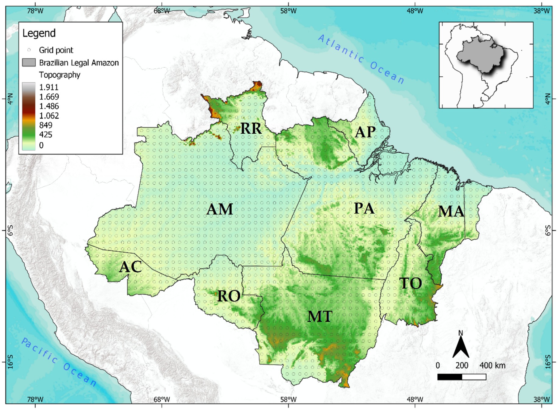
Figure 1. Geographical location of the Brazilian Legal Amazon (BLA) within South America, highlighting its topography, the abbreviations of each constituent state, and the spatial distribution of the observational rainfall grid points across the region.

2.2 CMIP6 model

The daily precipitation data simulated by the MPI model were obtained from the Earth System Grid (ESG) data portal, which hosts outputs from 23 CMIP6 models,¹ including historical simulations spanning the period from 1950 to 2014. As detailed in (Gutjahr et al., 2019), the high-resolution (HR) version, MPI-ESM1-2-HR, features a significantly enhanced horizontal resolution compared to its predecessor, the low-resolution (LR) version (MPI-ESM1.2-LR). Specifically, the HR version doubles the horizontal resolution of the ECHAM6.3 atmospheric components (T127, 0.9° × 0.9° or approximately 100 km) (Hertwig et al., 2015; Mauritsen et al., 2019). The ocean component has a resolution of 0.4° (approximately 40 km), implemented on a tripolar grid that allows for the explicit simulation of oceanic eddies (Jungclaus et al., 2013). This represents a substantial improvement over the LR configuration, which employs an atmospheric resolution of ~200 km and an oceanic resolution of 1.5°.

For CMIP6, the configurations used for ensemble members are designated by four indices, each representing specific model attributes: “r” denotes the realization, “i” the initialization, “p” the physical parameterization, and “f” the forcing. The ensemble identifier “r1i1p1f1” indicates that all members share the same initialization and physical configuration, with the forcing term “f1” corresponding to single-moment aerosol (OMA) simulations within the framework of the Atmospheric Model Intercomparison Project (AMIP) (Jungclaus et al., 2019).

2.3 Climate simulations

The Regional Climate Model version 4.7.1 (REG), configured in its hydrostatic variant with a horizontal resolution of 25 km, 23 vertical levels, and a model top at 50 hPa, was employed to conduct regional simulations for the historical period from 1980 to 2012. The initial and boundary conditions for these simulations were derived from the MPI model. It is important to note that the first year of simulation was designated as a ‘spin-up’ period to allow model stabilization and was therefore excluded from subsequent analyses.

The Community Land Model version 4.5 (CLM4.5) was coupled to REG to simulate processes at the soil–plant–atmosphere interface. Simulations were performed using the Mercator Normal projection, with a temporal resolution (time step) of 30 min and grid dimensions comprising 145 points in the Y direction and 240 points in the X direction.

For cumulus convection parameterization, the Tiedtke scheme (Tiedtke, 1996) was applied over continental regions, while the Kain–Fritsch scheme (Kain and Fritsch, 1990; Kain, 2004) was used over oceanic areas. Sub-grid scale cloud processes were represented using the explicit humidity scheme (SUBEX) (Pal et al., 2000). The Holtslag scheme (Holtslag et al., 1990) was employed for parameterizing the planetary boundary layer (PBL). The simulation domain encompasses part of South America and the South Atlantic Ocean, fully covering the Brazilian Legal Amazon (BLA), as illustrated in Figure 2.

Figure 2

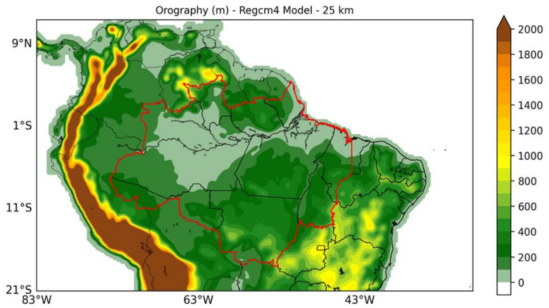
Figure 2. Domain and topography (in meters) utilized in the REG climate simulations at a horizontal resolution of 25 km. The red solid line delineates the extent of the Brazilian Legal Amazon (BLA).

2.4 Bias correction methods

We applied the Canonical Correlation Analysis (CCA) and Principal Component Regression (PCR) techniques, widely employed for generating seasonal climate forecasts (Mason and Tippett, 2017; Esquivel et al., 2018; Hossain et al., 2019), to evaluate which method more effectively corrects biases between the MPI and REG data relative to historical observations. Both techniques were applied to monthly data, relating raw monthly precipitation forecasts from the dynamic model to corresponding observations within a hindcast period (Barnett and Preisendorfer, 1987; Barnston, 1994; Johansson et al., 1998), following the procedure described in (Barnston and Tippett, 2017; see their Figure 1).

As described by Barnston and Tippett (2017), techniques such as CCA and PCR have been employed in different ways in the field of climate forecasting, either as purely statistical forecasting models that relate some anomaly pattern, such as sea surface temperature, to observed precipitation anomalies for a given month or season, or, as adapted for this study, by relating the raw output of the dynamical model to the corresponding observations. CCA is used to identify relationships between two multivariate sets of variables (vectors) by analyzing their cross-covariance matrices, aiming to find the optimal linear combination between the two sets that yields the highest correlation. PCR is a regression analysis technique based on principal component analysis. Typically, it involves regressing the outcome (also known as the response or dependent variable) on a set of covariates (also known as predictors, explanatory variables, or independent variables) using a standard linear regression model, but it employs PCA to estimate the unknown regression coefficients in the model. The datasets are standardized to ensure that all grid points from the models (predictors) and from the observations (predictands) have an equal opportunity to contribute to the forecasting process (Barnston, 1994).

The monthly precipitation totals derived directly from the MPI, as well as from its regionalized version (REG), served as predictors (X), while the corresponding monthly observed precipitation fields were considered predictands (Y). Both datasets were pre-processed using Empirical Orthogonal Function (EOF) analysis to reduce noise (Horel, 1981). In this procedure, EOFs for X and Y were computed separately, retaining approximately 70 to 80% of each variable’s original variance through a selected number of eigenvectors. This step ensures that CCA and PCR emphasize the dominant modes of variability in X and Y. Subsequently, a cross-correlation matrix was constructed from the principal component time series of X and Y, with its dimensions reduced to match the number of retained modes, from which canonical eigenvectors and eigenvalues were derived for both variables. Figure 3 provides a schematic illustration of the steps required to simulate observed precipitation (predicting Y) as a function of the accumulated precipitation fields from the models, MPI and REG (predictor X).

Figure 3

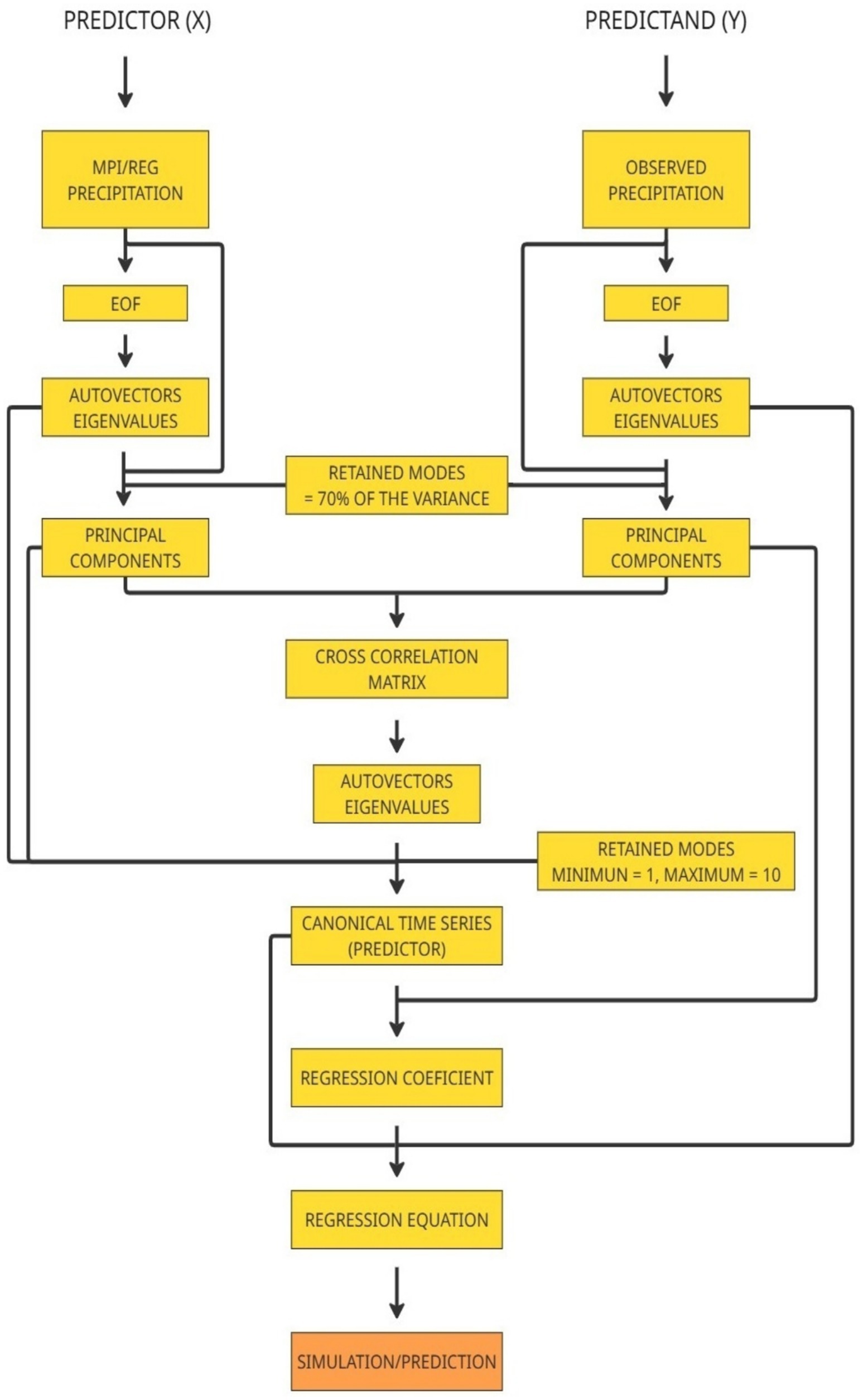
Figure 3. Schematic representation of the procedures applied to correct the occurrence bias in MPI/REG using observed occurrences as reference.

All CCA and PCR procedures were performed using the Climate Predictability Tool (CPT), developed by the International Research Institute for Climate and Society (IRI, 2019), a widely adopted software for processing large datasets in statistical seasonal climate prediction (Lucio et al., 2010; Kipkogei et al., 2017; Landman et al., 2019; da Rocha Júnior et al., 2021; Lucas et al., 2022; Silva et al., 2024). Barnston and Tippett (2017) demonstrated that, beyond constructing purely statistical forecast models, CCA and PCR can be applied to recalibrate and correct biases in raw outputs from dynamic models by associating hindcast predictions with observed data, enabling subsequent bias correction in future projections. Comprehensive guidance on CPT’s application for seasonal forecasts is available at: https://iri-pycpt.github.io/PyCPT2-Seasonal-Forecast-User-Guide/cpt.html.

For CCA, the analysis was initially configured to consider 10 modes, as recommended by the Climate Predictability Tool (CPT), which enables the software to automatically determine the optimal number of modes based on a model goodness-of-fit index. The regression equation derived from the canonical modes transforms the canonical temporal function of the predictor into that of the predictand. In contrast, PCR (Hotelling, 1957; Kendall, 1975) employs regression to establish combinations between predictor and predictand, effectively addressing typical challenges of Multiple Linear Regression, such as multicollinearity, while also reducing model noise. Further mathematical details on the application of PCR can be found in Rencher (2002) and Izenman (2008).

2.5 Evaluation methodology

The horizontal resolutions of the data sources differ: MPI has a spatial resolution of 0.9° × 0.9°, REG approximately 0.25° × 0.25°, and OBS 0.1° × 0.1°. To facilitate intercomparison between MPI and REG relative to OBS, and to standardize the input for the CCA and PCR experiments, all datasets were regridded to an intermediate resolution of 0.5° × 0.5° using bilinear interpolation. This approach is common and recommended in historical experiments involving HighResMIP models (Dong and Dong, 2021).

The precipitation data at this new resolution were subsequently aggregated into monthly totals at each grid point (1,695 points) for the reference period 1981–2012. From these, monthly, seasonal, and annual climatologies were computed to evaluate the performance of the simulated data relative to OBS. The metrics employed for this assessment were Pearson’s correlation coefficient (r), mean absolute error (MAE), and root mean square error (RMSE).

RMSE offers the advantage of penalizing larger errors more heavily, making it particularly appropriate for evaluating discrepancies between simulated precipitation from MPI and REG, as well as from the bias-corrected outputs generated via CCA and PCR. Its use is especially pertinent given the inherent heterogeneity of precipitation across the BLA throughout the year (Guo et al., 2021; Salazar et al., 2024). Lower MAE and RMSE values indicate a closer fit to the observations, whereas higher values reflect greater divergence. The mathematical formulations of r, MAE, and RMSE are presented below (Equations 1–3).

$\begin{array}{ll}r=\frac{cov(o,s)}{\sigma (o,s)}& (1)\end{array}$

$\begin{array}{ll}\mathit{MAE}=\frac{1}{n}{\sum }_{i=1}^n\mid s_I-o_I\mid & (2)\end{array}$

$\begin{array}{ll}\mathit{\text{RMSE}}=\sqrt{\frac{1}{n}{\sum }_{i=1}^n{(s_i-o_i)}^2}& (3)\end{array}$

where n is the total number of elements in the series, s_i = precipitation simulated (s) by the model in each monthly i, o_i = precipitation observed in each monthly i, Cov(o, s) is the covariance between the data, σ(o, s) is the respective standard deviation between the data, and μ is the mean of the observations.

To assess whether these r values genuinely reflect agreement between model estimates and observations, the parametric Student’s t-test was applied to verify the statistical significance of the correlations at the 95% confidence level (p-value < 0.05). Based on the sample sizes, a critical correlation coefficient of approximately 0.4 was determined; thus, correlations equal to or above this threshold can be considered statistically significant. However, it is important to note that statistical significance does not imply that model estimates and observations are necessarily close in magnitude, as substantial relative errors may still coexist with high correlation values.

In studies comparing observed and model-simulated data, jointly analyzing MAE and RMSE offers the advantage of quantifying simulation errors in the same units as the observed data. MAE measures the average magnitude of errors, providing an intuitive assessment of model accuracy without being disproportionately affected by outliers. However, due to the absolute value operator in its formulation, MAE may sometimes be confounded with systematic bias, especially when the errors predominantly occur in one direction. In contrast, RMSE penalizes larger errors more heavily, increasing sensitivity to significant discrepancies between observations and simulations.

After analyzing the skill with the metrics described above, in order to more accurately verify the gain of the MPI-CCA, MPI-PCR, REG-CCA and REG-PCR simulations versus their original versions, we calculated the Kling-Gupta Efficiency (KGE), whose limits range from −∞ to 1, with values close to 1 indicating the best model performances (Gupta et al., 2009). This metric is widely used in hydrological model evaluations (Towner et al., 2019), but it is versatile enough to assess any type of model simulation. The KGE combines three key components: linear correlation, bias ratio, and relative variability, into a single index. Its values range from −∞ to 1, with values closer to 1 indicating better agreement between observations and simulations (Equation 4).

KGE thresholds are often used subjectively. Knoben et al. (2019) showed that for a hypothetical case where a model demonstrates a correlation equal to 0 in relation to the observations, with simulated standard deviation also equal to 0 and mean of the simulations equal to that of the observations, despite varying from −∞, a good starting point to assess whether the model’s performance is satisfactory would be from −0.41 to 1, with values lower than −0.41 indicating poor model performance. In this case, we adapted the division of KGE values suggested by (Kling et al., 2012) into four categories, as follows: “excellent” (KGE ≥ 0.75); “very good” (0.75 > KGE ≥ 0.5); “intermediate” (0.5 > KGE ≥ 0); “bad” (0 > KGE > − 0.41); “very bad” (KGE ≤ − 0.41).

$\begin{array}{ll}\mathit{KGE}=1-\sqrt{{(r-1)}^2+{(\alpha -1)}^2+{(\beta -1)}^2}& (4)\end{array}$

where 𝑟 is the linear correlation between observations and simulations, 𝛼 a measure of the relative variability between observations and simulations given by the ratio between their standard deviations: $\frac{{\sigma }_s}{{\sigma }_0}$ , and 𝛽 a bias term given by the ratio between the averages of the sets of observations and simulations: $\frac{{\mu }_s}{{\mu }_o}$ .

3 Results and discussions

3.1 Precipitation patterns and model bias

The BLA comprises six homogeneous rainfall regions (dos Santos Silva et al., 2023), marked by two distinct rainy seasons, December to February in the south, influenced by the Chaco Low and the South Atlantic Convergence Zone (SACZ), and April to June in the north, driven by the Intertropical Convergence Zone (ITCZ). The central-southern BLA experiences a more intense dry season during winter (June to August), while the far north sees a milder dry period in spring (September to November) (Marengo and Nobre, 2009; Firpo et al., 2022). These seasonal rainfall patterns are illustrated in Figure 4 through monthly climatologies of observed precipitation compared with simulations from MPI and REG, including bias maps that highlight discrepancies between model outputs and observations.

Figure 4

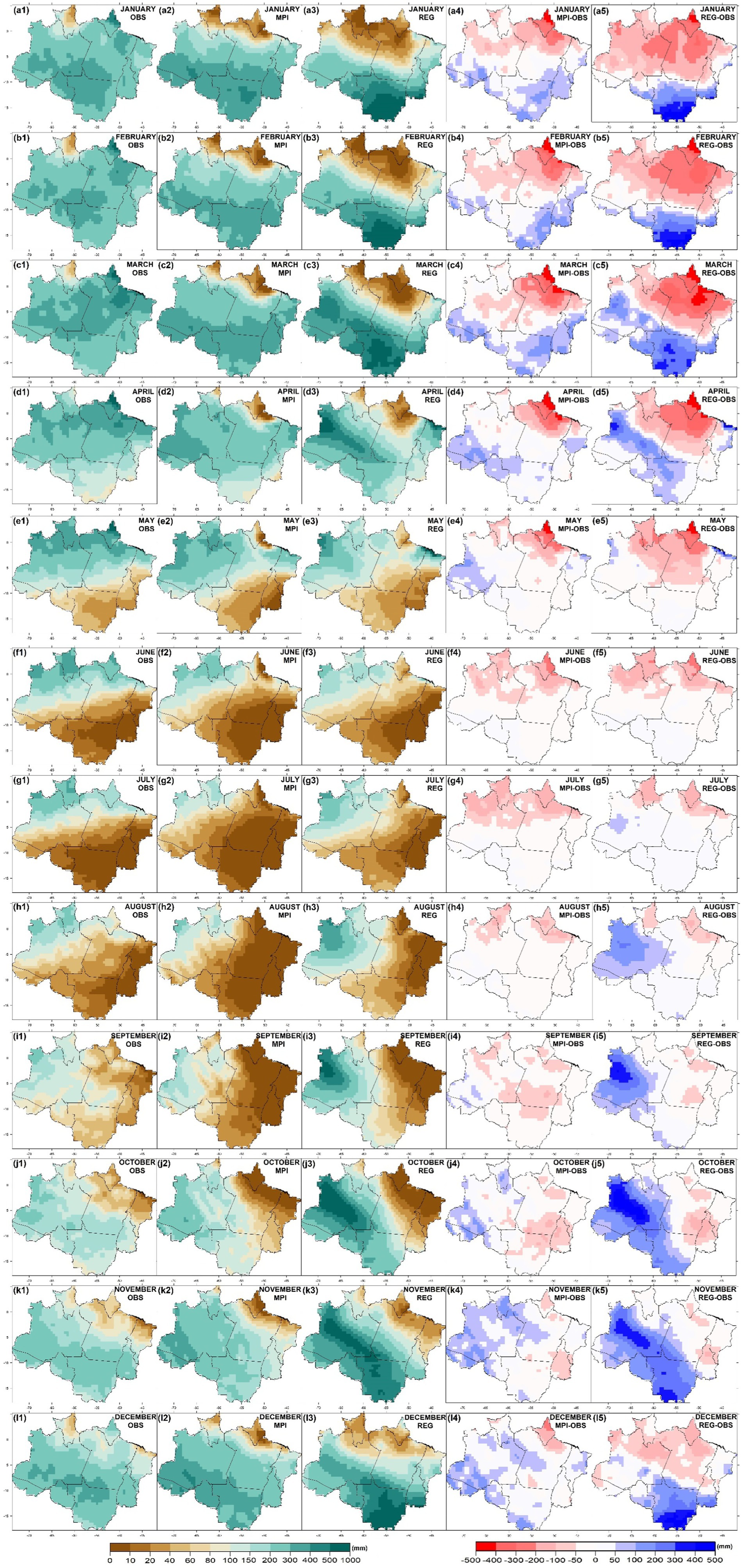
Figure 4. Monthly mean precipitation (1981–2012) in the first three columns: observed data, MPI, and REG simulations, respectively (mm month⁻¹). The fourth and fifth columns show the respective deviations of MPI and REG from the observed means (mm month⁻¹). From top to bottom: January (a1–a5), February (b1–b5), March (c1–c5), April (d1–d5), May (e1–e5), June (f1–f5), July (g1–g5), August (h1–h5), September (i1–i5), October (j1–j5), November (k1–k5), and December (l1–l5). The BLA region spans from 5.3°N to 13.7°S latitude and from 74°W to 45.68°W longitude.

The historically higher rainfall concentration in the central-southern BLA between January and March (Figures 4a1–a3,b1–b3,c1–c3) is generally overestimated by MPI, whereas precipitation in the northern BLA during this period tends to be under-estimated (Figures 4a4,b4). From April to May, this pattern diminishes slightly, with negative biases persisting in the northern areas of RR, PA, and AP, while positive biases are more localized in the western parts of AM and AC (Figures 4d1–d4,e1–e4). During the winter and early spring months (June to September), underestimations are evident in northern BLA, although with lesser intensity than earlier in the year (Figures 4f1–f4,i1–i4). Between October and December (Figures 4j1–j4 to Figures 4l1–l4), MPI increasingly overestimates precipitation over the central-western BLA, while underestimations become confined mainly to AP.

The REG model amplifies these MPI-simulated patterns, exhibiting more intense magnitudes of both positive and negative biases across the BLA. Notably, REG shows significant positive biases over MT from January to March and again from October to December, alongside pronounced negative biases in northern BLA from January to May (Figures 4a5,b5,c5,d5,e5,j5,k5,l5). In June and July, REG’s climatological behavior closely mirrors MPI, but from August to December, REG displays a broader area with positive biases, particularly over AM, where a core of overestimation emerges in August and intensifies through December (Figures 4h5,i5,j5,k5,l5).

Overall, both MPI and REG exhibit a dipolar bias pattern across the BLA, with negative biases predominating in the north and east, and positive biases in the south and west (Firpo et al., 2022; Ferreira et al., 2023). These findings align with previous assessments of CMIP6 historical simulations for the Amazon, which attribute this pattern to deficiencies in the models’ representation of cloud physics, notably the misplacement of the Amazon’s maximum precipitation center (Khairoutdinov et al., 2005), an issue persisting from earlier CMIP versions (Yin et al., 2013; Sierra et al., 2015; Ortega et al., 2021; Dias and Reboita, 2021).

Given its higher spatial resolution compared to MPI, one would expect REG to exhibit superior performance. However, regional models can inherit, amplify, or even generate their own biases (Dosio et al., 2015; Takayabu et al., 2016), due to inconsistencies between the circulation patterns simulated by the regional model and those imposed by the boundary conditions of the global model. These inconsistencies may stem from the relative importance of large-scale forcing versus local-scale phenomena, as well as from the difference in domain size between the regional and global models, REG operating at 25 km and MPI at approximately 100 km, which may allow REG to generate a substantial portion of its variability internally and in an unforced manner (Nikiema et al., 2017; Sanchez-Gomez and Somot, 2018). Other factors that may limit the regional model’s performance relative to the global model include the simplified representation of key processes, such as ocean–atmosphere coupling, since sea surface temperatures (SSTs) are obtained from global simulations or reanalyses, and cloud–aerosol interactions, which are often included in regional models using climatological values. A noteworthy aspect was REG’s underestimation of accumulated precipitation along the coastal region from January to June, particularly between the states of Amapá and Pará, and its overestimation in the western and southern parts of the BLA from August to December, clearly amplifying patterns that were already present in MPI, albeit with lower intensity.

Despite these biases, MPI and REG successfully reproduce the BLA’s annual precipitation cycle, including the characteristic dipole between northern and southern sectors during the driest months (May to October). Similar behavior has been reported in other CMIP6 models, such as the Chinese BCCCSM2MR/BCCESM1 (Wu et al., 2019), the Canadian CANESM5 (Swart et al., 2019), the American CESM2/CESM2WACCM (Gettelman et al., 2019), E3SM10 (Golaz et al., 2019), GIS-SE21G/GISSE21H (Kelley et al., 2020), and the European EC-Earth3/EC-Earth3Veg (Doblas Reyes et al., 2018), all showing considerable underestimations in the extreme north and northeast of the BLA (RR, PA, AP, and MA), significantly reducing rainfall estimates even during peak rainy months, as confirmed by observational data.

3.2 Model performance metrics before bias correction

Figure 5 illustrates the spatial distribution of average monthly correlation coefficients (r) (Figures 5a,b). For both models, the highest correlations are found in the northeastern and central-southern sectors of the BLA, fully encompassing the states of Acre (AC), Rondônia (RO), Mato Grosso (MT), Tocantins (TO), and Maranhão (MA), as well as parts of Amazonas (AM) and Pará (PA). MPI generally exhibits higher correlation values and a broader area with r greater than 0.4 compared to REG.

Figure 5

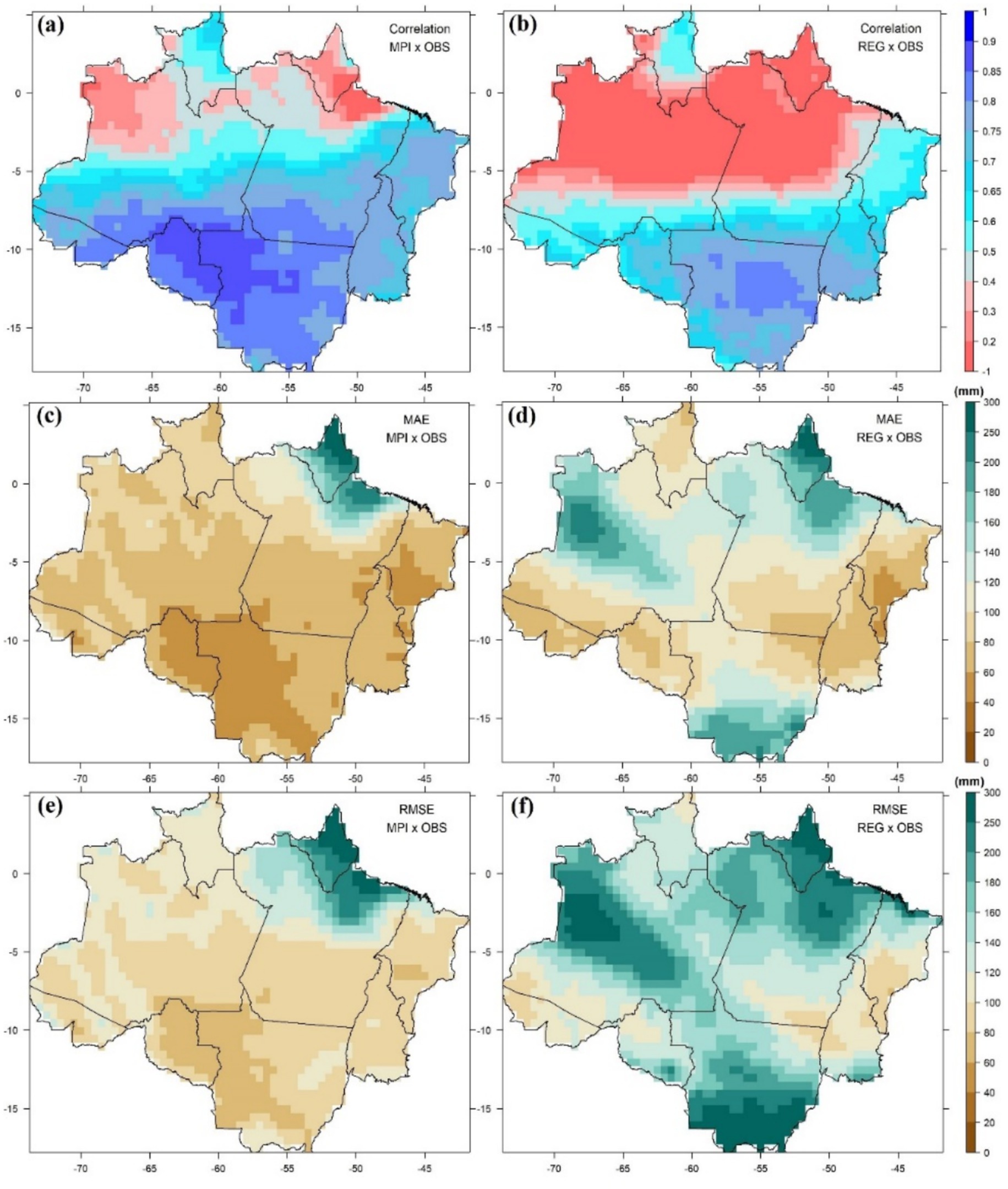
Figure 5. Spatial distribution of Pearson correlation coefficients between model outputs and observations before bias correction: (a) MPI and (b) REG. Mean Absolute Error (MAE) before bias correction for: (c) MPI and (d) REG. Root Mean Square Error (RMSE) before bias correction for: (e) MPI and (f) REG.

An important feature of these correlation fields is that the highest values correspond to BLA sectors where MPI and REG most effectively captured seasonal variability, notably in the state of RR, which exhibits a well-defined seasonal cycle characterized by a rainy period during austral autumn and winter, and a dry period during summer, as previously shown in Figure 4. Conversely, the lowest MPI correlations are observed in the western Amazon, where the seasonal cycle is less pronounced due to consistently high rainfall year-round. The REG further expands this region of low correlations into the central-northern part of PA. Similar patterns have been reported in previous studies evaluating the performance of various rainfall estimation datasets for the BLA (Sapucci et al., 2022; dos Santos Silva et al., 2023).

Figure 5 also presents the spatial distribution of MAE (Figures 5c,d) and RMSE (Figures 5e,f) for the MPI and REG simulations. The importance of jointly evaluating these metrics becomes evident through the spatial patterns. For MPI, the highest MAE values are concentrated in a limited area of the northern BLA, between the states of AP and PA (Figure 5c). In the case of REG (Figure 5d), in addition to this region, two other significant areas of high MAE emerge: one in the western part of AM and another in the southern part of MT.

When analyzing RMSE, the spatial extent of the errors increases. For MPI (Figure 5e), a broader area of high errors is evident in northern BLA, surpassing what is indicated by MAE alone. For REG (Figure 5f), regions that initially appeared fragmented in the MAE maps become clearly interconnected, revealing more coherent zones of high error across the western and southern BLA.

Across the entire study region, MPI exhibited an average MAE of 80 mm/month and an RMSE of 97 mm/month. These findings are consistent with previous research, Monteverde et al. (2022) reported an average RMSE of 68 mm/month for a set of models in northern BLA (excluding the specific MPI version used here) and approximately 40 mm/month for the southern BLA. This supports both the values found in our analysis and the observed gradient, with higher RMSE in the north compared to the south. Similarly Dias and Reboita (2021), in their evaluation of CMIP6 models (including MPI), noted that both the lower-resolution MPI-ESM1-2-LR and higher-resolution versions ranked among the best-performing models for tropical South America, including the BLA. These corroborate our results and further validate the choice of using the high-resolution MPI version for bias correction in this study.

Overall, the results in Figure 5 indicate low correlations and higher errors predominantly in the north-central and western portions of the BLA, precisely the region characterized by its highest rainfall. While models with spatial resolutions around 100 km, such as the MPI used here, represent significant progress in global climate modeling, they still face limitations in adequately representing the physical processes driving rainfall, especially those linked to warm cloud formation and maintenance (Fan et al., 2018; Shrivastava et al., 2019; Pendharkar et al., 2023). Given that precipitation from warm clouds constitutes a substantial portion of total rainfall in these BLA sub regions, model deficiencies in simulating evapotranspiration and overestimating wind speeds over the Amazon canopy can impair atmospheric process representation and, consequently, precipitation simulation accuracy.

In the case of REG, the discrepancies are further exacerbated by the choice of cumulus parameterization, which presents inherent limitations in representing tropical convection processes and, consequently, the intensity and spatial distribution of rainfall (dos Santos Silva et al., 2023). Initially, a deterioration in the results obtained from MPI was not expected; however, as noted in Section 3.1, it is not uncommon for dynamic downscaling using regional models to fail to improve global model outputs, particularly under certain conditions where local-scale phenomena, critical to the annual precipitation cycle, are not well represented. In any case, using REG outputs in the face of bias amplification relative to MPI, and the resulting increase in precipitation estimation errors across the BLA, became both a challenge and a key objective of this research. The aim was to assess whether, even under such conditions, bias correction techniques would still be effective in adjusting the outputs of both models to better match observed data.

3.3 Bias correction using CCA and PCR and performance metrics

As demonstrated by Barnston and Tippett (2017), techniques such CCA can be applied to correct biases in climate forecasts derived from dynamic models, enhancing the correlation between observations and hindcasts, thereby improving the reliability of both retrospective and future projections. Given that PCR is conceptually similar to CCA, it is reasonable to expect that it could serve the same purpose.

Figure 6 illustrates the spatial loadings of the first mode of variability for the predictor (X) and predictand (Y), in this case, MPI-simulated and observed rainfall, respectively, using January as an example (Figures 6a,b). This first mode represents the dominant component of the correlation between MPI and observations, indicating that positive canonical loadings associated with above-average precipitation in MPI correspond to above-average observed rainfall across much of the central-eastern BLA, though areas of inverse association are also evident. The canonical correlation for this variable pair was 0.78, with the first mode explaining over 40% of the variance in observed rainfall.

Figure 6

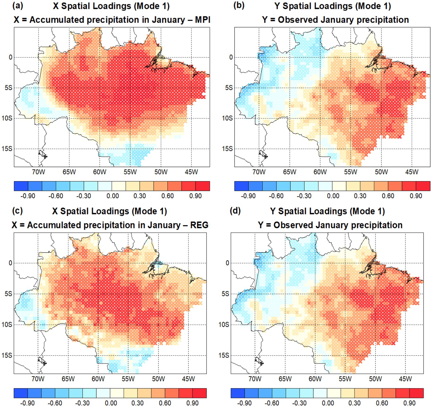
Figure 6. Spatial loadings of predictor (X) and predictand (Y) for the first mode, showing the dominant correlation pattern in January precipitation between (a) MPI model data and (b) observations. Panels (c) and (d) show the analogous patterns for the REG model and observations, respectively.

Similarly, for the REG model and observed precipitation (Figures 6c,d), the first mode also emerged as the most dominant, displaying a comparable spatial pattern to that seen with MPI. However, in this case, the positive canonical loadings associated with above-average observed precipitation were more concentrated in the central BLA. The canonical correlation for this pair was 0.84, with the first mode explaining more than 30% of the variance in observed rainfall. According to Lima et al. (2020), retaining modes of variability that cumulatively explain over 70% of the variance in the data is generally sufficient for constructing a predictive statistical model, as incorporating additional modes may introduce noise without necessarily enhancing predictive skill.

Figure 7a shows that for MPI (predictor X), the first five modes explain a total of 77% of the variance, distributed as follows: 43% for the first mode, 14% for the second, 10% for the third, 6% for the fourth, and 4% for the fifth. Correspondingly, Figure 7b shows the variance explained in observations (predictand Y) for the same five modes. The pattern is consistent with the MPI modes but with lower percentages: 22, 19, 7, 6, and 4%, respectively. This means that the 77% of variance explained by the MPI modes accounts for about 58% of the variance in observed precipitation.

Figure 7

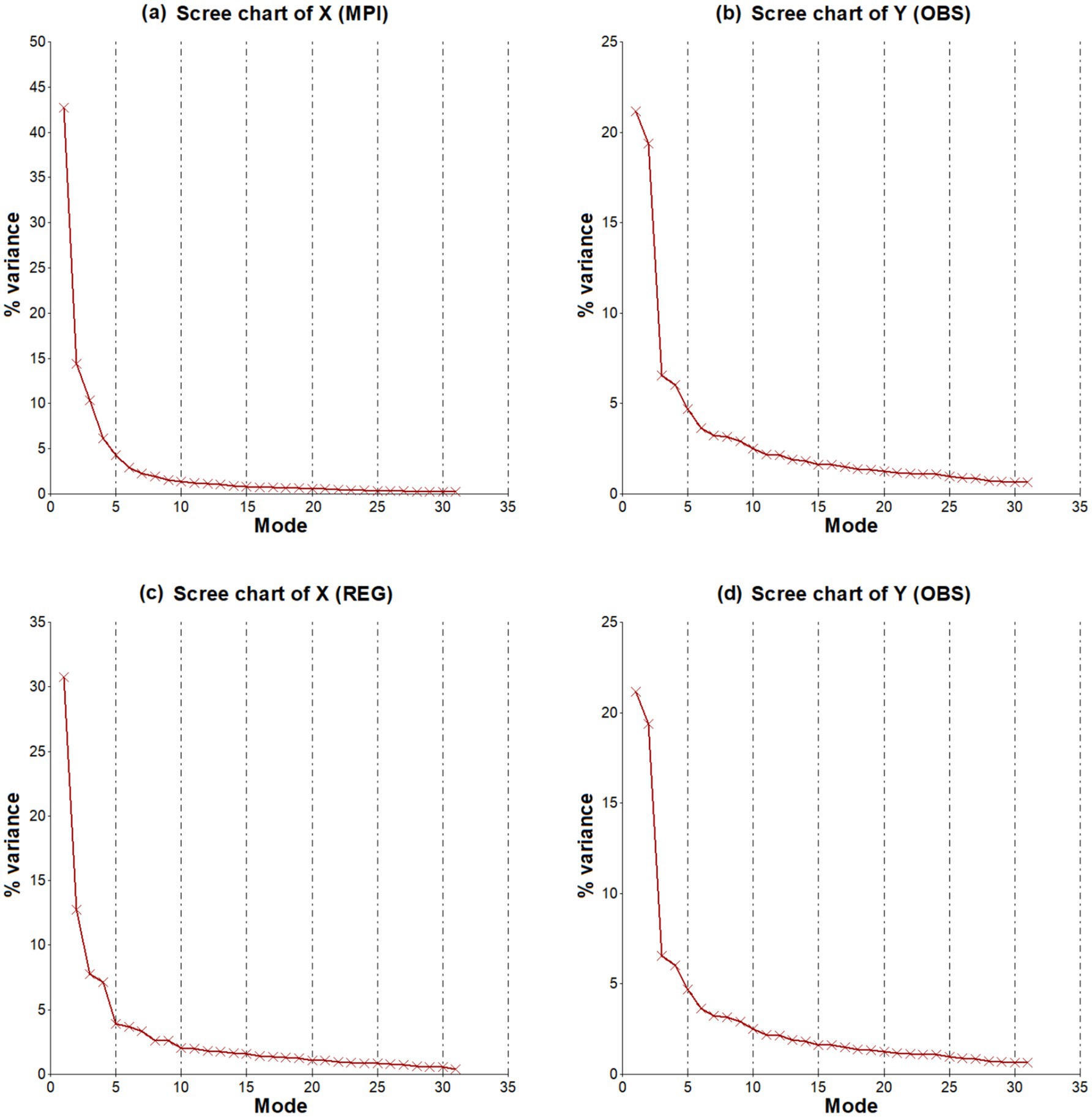
Figure 7. Scree plots showing the variance explained by the number of modes retained in the principal component analysis for (a) MPI and (b) observations (OBS), and similarly for (c) REG and (d) OBS.

Similarly, for REG, Figure 7c indicates that the first five modes explain 63% of the variance in the model data, with 31, 13, 8, 7, and 4% attributed to modes one through five, respectively. Figure 7d shows the corresponding explained variance in observations, also consistent with the REG modes but with lower values: 22, 14, 7, 6, and 4%. Thus, the 63% variance explained by REG corresponds to approximately 53% of the observed variance.

The correction of historical biases in MPI and REG models yielded highly satisfactory improvements, demonstrated by significantly increased correlations and reduced errors. Tables 1, 2 present monthly comparisons of correlation, MAE, and RMSE for MPI before and after correction (MPI-CCA and MPI-PCR), and similarly for REG. The PCR method outperformed CCA in 11 out of 12 months, except for May, where CCA was superior. Notably, bias corrections applied to REG showed better performance in 9 months, while direct corrections on MPI were more effective in only 3 months. This highlights the effectiveness of bias correction methods, especially for REG, which initially showed poorer climatological and error metrics compared to MPI. Table 3 summarizes the mean values for the BLA, indicating the best-performing models and correction methods, highlighted in shades of gray in Tables 1, 2.

Table 1

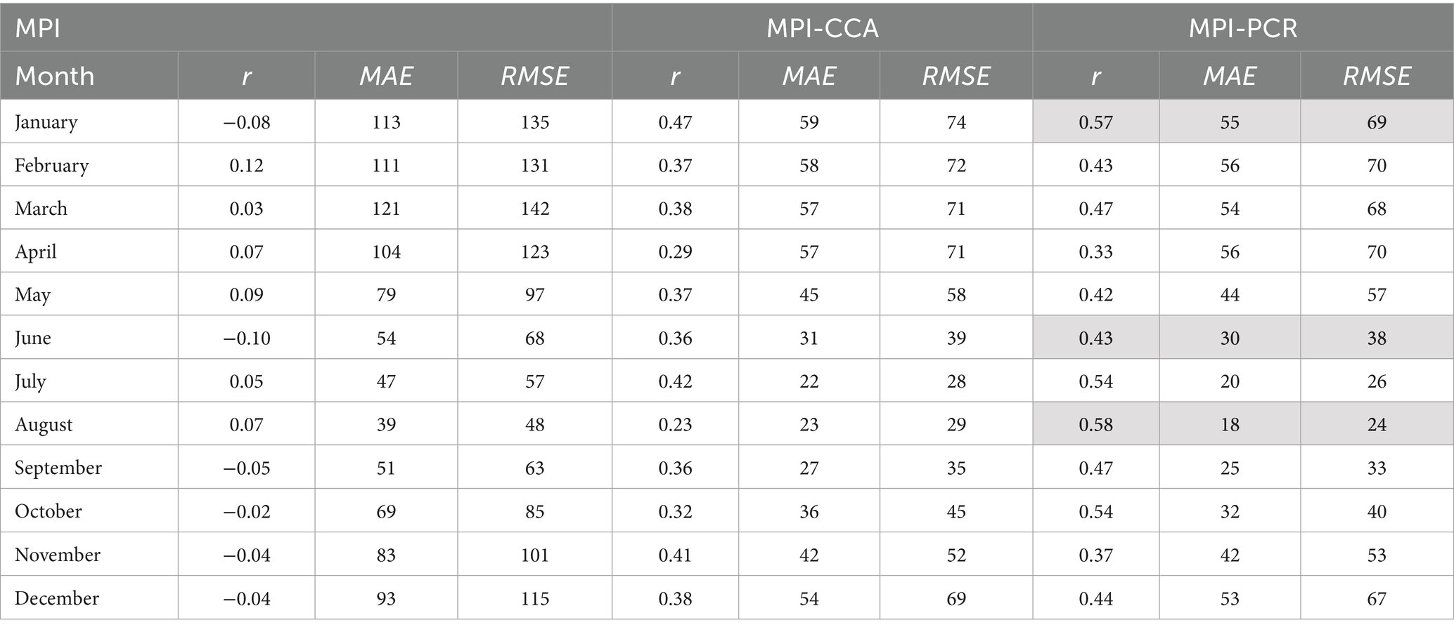
Table 1. Monthly Pearson correlation coefficient (r), mean absolute error (MAE in mm), and root mean square error (RMSE in mm) comparing MPI raw simulations, MPI bias-corrected with Canonical Correlation Analysis (MPI-CCA), and MPI bias-corrected with Principal Component Regression (MPI-PCR) against observed precipitation averages.

Table 2

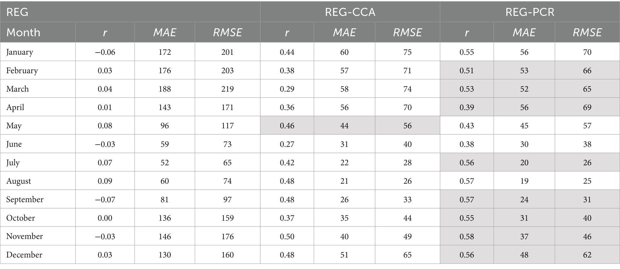
Table 2. Monthly Pearson correlation coefficient (r), mean absolute error (MAE in mm), and root mean square error (RMSE in mm) comparing REG raw simulations, REG bias-corrected with Canonical Correlation Analysis (REG-CCA), and REG bias-corrected with Principal Component Regression (REG-PCR) against observed precipitation averages.

Table 3

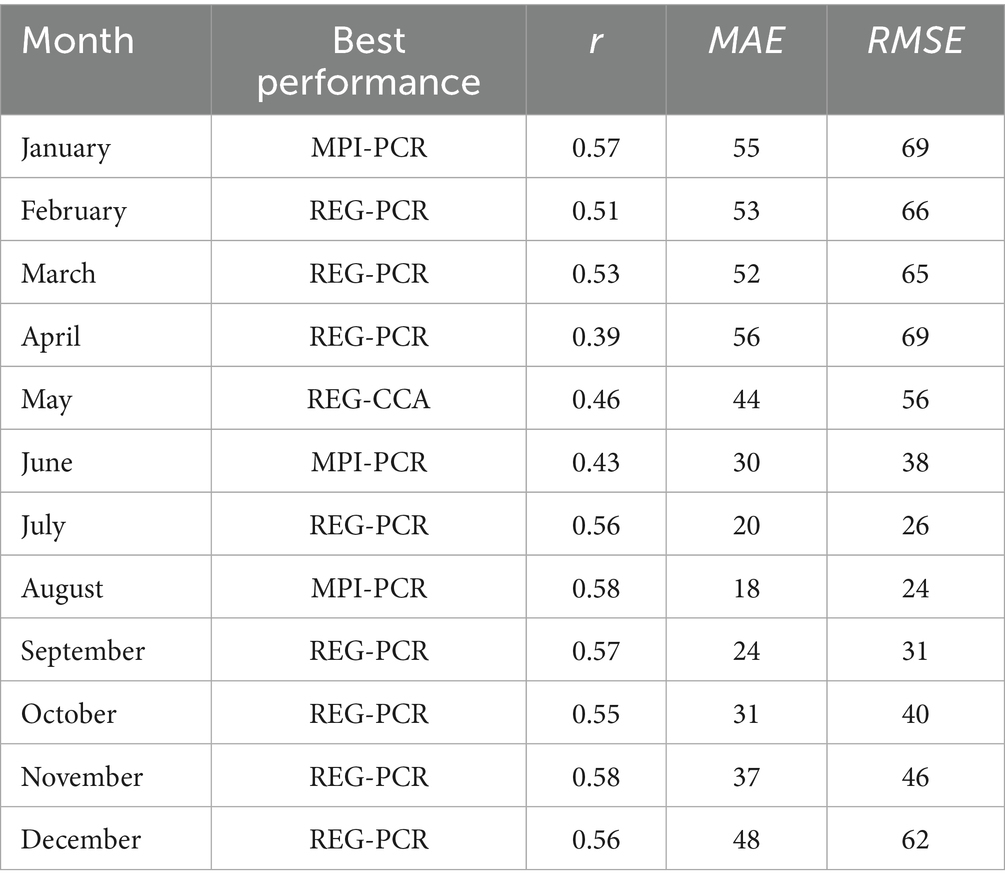
Table 3. Summary of the best-performing bias correction method for each month applied to MPI and REG models, showing the corresponding Pearson correlation (r), mean absolute error (MAE in mm), and root mean square error (RMSE in mm).

PCR prioritizes components that account for the greatest variance in the predictor variables, which can enhance predictive performance. In contrast, CCA aims to maximize the correlation between two sets of variables, even if this involves components with low variance, thus potentially conveying less informative content for data explanation. Moreover, PCR is generally simpler to implement and interpret, especially when the goal is to predict a dependent variable based on a set of predictors. CCA, on the other hand, often requires more complex interpretation, as it involves pairs of canonical variables that represent linear combinations from two distinct sets (X and Y), which may not always carry clear practical significance. Nonetheless, CCA has advantages in contexts where the primary aim is not prediction but the exploration of relationships between two multivariate datasets, such as identifying coupled patterns (e.g., SST and precipitation). In climatology, CCA is particularly useful for detecting canonical patterns between spatial fields (Barnston, 1994; Jolliffe, 2002; Wilks, 2011).

Figure 8 illustrates the spatial distribution of KGE for MPI and REG simulations corrected by CCA and PCR, showing that both methods significantly improve precipitation estimates during the historical period, particularly in the center-south and eastern BLA, where KGE exceeds 0.75. While performance in western BLA (AM state) is lower, it generally remains “very good,” though some areas corrected by CCA fall below 0.5. These results indicate notable improvement over raw model outputs (Table 3), reinforcing that CCA and PCR effectively reduce biases in CMIP6 precipitation data and can be applied to future climate projections to reduce uncertainties. Despite advances in CMIP6 over CMIP5, substantial challenges remain, and bias correction techniques like CCA and PCR offer computationally efficient ways to enhance model reliability for various applications (Taylor et al., 2012; Eyring et al., 2015; Navarro-Racines et al., 2020; Di Virgilio et al., 2022; Fall et al., 2023; Risser et al., 2024).

Figure 8

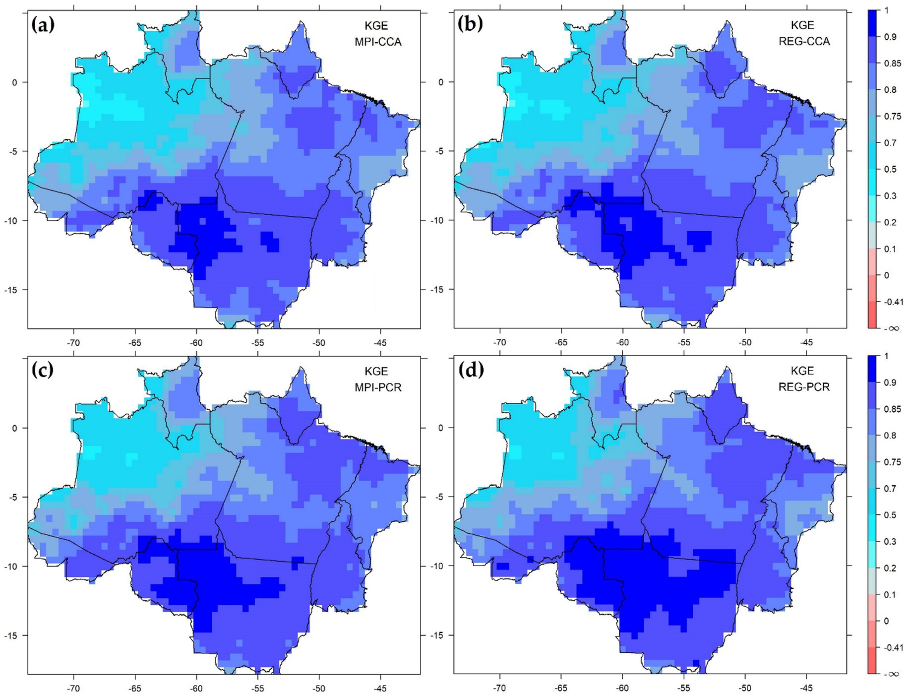
Figure 8. Spatial distribution of Kling-Gupta Efficiency (KGE) values for bi-as-corrected precipitation simulations over the BLA: (a) MPI-CCA, (b) REG-CCA, (c) MPI-PCR, and (d) REG-PCR.

4 Conclusion

This study evaluated precipitation estimates from the MPI-ESM1-2-HR (MPI) climate model over the Brazilian Legal Amazon (BLA), along with its dynamic downscaling using RegCM4.7.1 (REG) driven by MPI. Observed precipitation data from 1,695 locations (1981–2012) were compared to outputs from both MPI and REG, followed by bias correction using canonical correlation analysis (CCA) and principal component regression (PCR). The results showed that neither MPI nor REG accurately reproduced the annual precipitation cycle. MPI exhibited significant biases, overestimating rainfall in the southern BLA and underestimating it in the northern region. REG not only failed to correct these biases but also amplified errors and reduced the correlation with observations.

Despite this, both CCA and PCR bias correction methods substantially improved precipitation estimates. PCR outperformed CCA in 11 out of 12 months across all metrics (correlation, MAE, and RMSE), and REG-PCR delivered the best results in 8 of the 12 months. Kling-Gupta Efficiency (KGE) analysis also confirmed the overall superiority of REG-PCR compared to other combinations. Therefore, the recommended approach is to use REG for dynamic regionalization of CMIP models, followed by bias correction, preferably with PCR, or alternatively with CCA. This combination effectively reduces historical biases and offers a robust method for improving future climate projections under various greenhouse gas emission scenarios.

Finally, it is important to highlight the advantages and disadvantages of using bias correction techniques. Among the advantages, bias correction adjusts systematic deviations in climate models, improves statistical indicators (such as mean, variance, and correlation), reduces uncertainties in future projections, and enables the direct use of simulations in impact models, all with low computational cost through techniques such as CCA and PCR. Among the disadvantages, bias correction assumes the stationarity of historical biases, which may not hold under significant climate change, may have limitations in correcting extreme events, and critically depends on the quality and coverage of observational data, particularly in poorly monitored regions such as parts of the Amazon. Therefore, robust gridded observational analyses, such as the one used in this study, are recommended.

Data availability statement

The raw data supporting the conclusions of this article will be made available by the authors, without undue reservation.

Author contributions

FS: Conceptualization, Data curation, Formal analysis, Methodology, Software, Validation, Visualization, Writing – original draft, Writing – review & editing. HG: Conceptualization, Formal analysis, Methodology, Visualization, Writing – original draft, Writing – review & editing. CC: Conceptualization, Formal analysis, Methodology, Visualization, Writing – original draft, Writing – review & editing. AN: Formal analysis, Writing – original draft, Writing – review & editing. IF: Software, Writing – review & editing. MHS: Software, Writing – review & editing. MCS: Formal analysis, Writing – review & editing. RC: Software, Writing – review & editing. JR: Software, Writing – review & editing. VS: Formal analysis, Writing – original draft, Writing – review & editing. AS: Formal analysis, Writing – original draft, Writing – review & editing. IS: Formal analysis, Writing – original draft, Writing – review & editing. RR: Software, Writing – review & editing. JC: Writing – review & editing. HS: Writing – review & editing. ES: Writing – review & editing. DS: Writing – review & editing. RT: Writing – review & editing.

Funding

The author(s) declare that financial support was received for the research and/or publication of this article. This research was funded by Instituto Tecnológico Vale (Project name: “Cenários de eventos extremos”).

Conflict of interest

The authors declare that the research was conducted in the absence of any commercial or financial relationships that could be construed as a potential conflict of interest.

Generative AI statement

The authors declare that no Gen AI was used in the creation of this manuscript.

Publisher’s note

All claims expressed in this article are solely those of the authors and do not necessarily represent those of their affiliated organizations, or those of the publisher, the editors and the reviewers. Any product that may be evaluated in this article, or claim that may be made by its manufacturer, is not guaranteed or endorsed by the publisher.

Footnotes

1. ^https://esgf-node.llnl.gov/search/cmip6/, accessed on 20 March 2024.

References

Almazroui, M., Ashfaq, M., Islam, M. N., Rashid, I. U., Kamil, S., Abid, M. A., et al. (2021). Assessment of CMIP6 performance and projected temperature and precipitation changes over South America. Earth Syst. Environ. 5, 155–183. doi: 10.1007/s41748-021-00233-6

Crossref Full Text | Google Scholar

Alvares, C. A., Stape, J. L., Sentelhas, P. C., de Moraes Gonçalves, J. L., and Sparovek, G. (2013). Köppen's climate classification map for Brazil. Meteorol. Z. 22, 711–728. doi: 10.1127/0941-2948/2013/0507

Crossref Full Text | Google Scholar

Ataide, W. L. S., Oliveira, F. A., and Pinto, C. A. D. (2020). Balanço de radiação, energia e fechamento do balanço em uma floresta prístina na Amazônia oriental. Rev. Bras. Geogr. Fís. 13, 2603–2627. doi: 10.26848/rbgf.v13.6.p2603-2627

Crossref Full Text | Google Scholar

Barnett, T. P., and Preisendorfer, R. (1987). Origins and levels of monthly and seasonal forecast skill for United States surface air temperatures determined by canonical correlation analysis. Mon. Weather Rev. 115, 1825–1850. doi: 10.1175/1520-0493(1987)115<1825:OALOMA>2.0.CO;2

Crossref Full Text | Google Scholar

Barnston, A. G. (1994). Linear statistical short-term climate predictive skill in the northern hemisphere. J. Clim. 7, 1513–1564. doi: 10.1175/1520-0442(1994)007<1513:LSSTCP>2.0.CO;2

Crossref Full Text | Google Scholar

Barnston, A. G., and Tippett, M. K. (2017). Do statistical pattern corrections improve seasonal climate predictions in the North American multimodel ensemble models? J. Clim. 30, 8335–8355. doi: 10.1175/JCLI-D-17-0054.1

Crossref Full Text | Google Scholar

Costa, C. P. W., and Satyamurty, P. (2016). Inter-hemispheric and inter-zonal moisture transports and monsoon regimes. Int. J. Climatol. 36, 4705–4722. doi: 10.1002/joc.4662

Crossref Full Text | Google Scholar

Costa, D. F., Gomes, H. B., Silva, M. C. L., and Zhou, L. (2022). The most extreme heat waves in Amazonia happened under extreme dryness. Clim. Dyn. 59, 281–295. doi: 10.1007/s00382-021-06134-8

Crossref Full Text | Google Scholar

Costa, R. L., Baptista, G. M. M., Gomes, H. B., Silva, F. D. S., Rocha Júnior, R. L., and Nedel, A. S. (2021). Analysis of future climate scenarios for northeastern Brazil and implications for human thermal comfort. An. Acad. Bras. Cienc. 93, 1–23. doi: 10.1590/0001-3765202120190651

Crossref Full Text | Google Scholar

da Rocha Júnior, R. L., Cavalcante Pinto, D. D., dos Santos Silva, F. D., Gomes, H. B., Barros Gomes, H., Costa, R. L., et al. (2021). An empirical seasonal rainfall forecasting model for the northeast region of Brazil. Water 13:1613. doi: 10.3390/w13121613

Crossref Full Text | Google Scholar

Dereczynski, C., Chou, S. C., Lyra, A., Sondermann, M., Regoto, P., Tavares, P., et al. (2020). Downscaling of climate extremes over South America—part I: model evaluation in the reference climate. Weather Clim. Extremes 29:100273. doi: 10.1016/j.wace.2020.100273

Crossref Full Text | Google Scholar

Dias, C. S., and Reboita, M. S. (2021). Assessment of CMIP6 simulations over tropical South America. Rev. Bras. Geogr. Fis. 14, 1282–1295. doi: 10.26848/rbgf.v14.3.p1282-1295

Crossref Full Text | Google Scholar

Di Virgilio, G., Ji, F., Tam, E., Nishant, N., Evans, J. P., Thomas, C., et al. (2022). Selecting CMIP6 GCMs for CORDEX dynamical downscaling: model performance, independence, and climate change signals. Earths Future 10:e2021EF002625. doi: 10.1029/2021EF002625

Crossref Full Text | Google Scholar

Doblas Reyes, F., Acosta Navarro, J. C., Acosta Cobos, M. C., Bellprat, O., Bilbao, R., Castrillo Melguizo, M., et al. (2018). Using EC-earth for climate prediction research. ECMWF. Newsletter Number 154, 35–40.

Google Scholar

Dong, T., and Dong, W. (2021). Evaluation of extreme precipitation over Asia in CMIP6 models. Clim. Dyn. 57, 1751–1769. doi: 10.1007/s00382-021-05773-1

Crossref Full Text | Google Scholar

Dosio, A., Panitz, H.-J., Schubert-Frisius, M., and Lüthi, D. (2015). Dynamical downscaling of CMIP5 global circulation models over CORDEX-Africa with COSMO-CLM: evaluation over the present climate and analysis of the added value. Clim. Dyn. 44, 2637–2661. doi: 10.1007/s00382-014-2262-x

Crossref Full Text | Google Scholar

dos Santos Silva, F. D., da Costa, C. P. W., dos Santos Franco, V., Gomes, H. B., da Silva, M. C. L., dos Santos Vanderlei, M. H. G., et al. (2023). Intercomparison of different sources of precipitation data in the Brazilian Legal Amazon. Climate 11:241. doi: 10.3390/cli11120241

Crossref Full Text | Google Scholar

Espinoza, J. C., Ronchail, J., Marengo, J. A., and Segura, H. (2019). Contrasting north-south changes in Amazon wet-day and dry-day frequency and related atmospheric features (1981–2017). Clim. Dyn. 52, 5413–5430. doi: 10.1007/s00382-018-4462-2

Crossref Full Text | Google Scholar

Esquivel, A., Llanos-Herrera, L., Agudelo, D., Prager, S. D., Fernandes, K., Rojas, A., et al. (2018). Predictability of seasonal precipitation across major crop growing areas in Colombia. Clim. Serv. 12, 36–47. doi: 10.1016/j.cliser.2018.09.001

Crossref Full Text | Google Scholar

Eyring, V., Bony, S., Meehl, G. A., Senior, C., Stevens, B., Stouffer, R. J., et al. (2015). Overview of the coupled model intercomparison project phase 6 (CMIP6) experimental design and organisation. Geosci. Model Dev. Discuss. 8, 10539–10583. doi: 10.5194/gmdd-8-10539-2015

Crossref Full Text | Google Scholar

Fall, P., Diouf, I., Deme, A., Diouf, S., Sene, D., Sultan, B., et al. (2023). Bias-corrected CMIP5 projections for climate change and assessments of impact on malaria in Senegal under the VECTRI model. Trop. Med. Infect. Dis. 8:310. doi: 10.3390/tropicalmed8060310

PubMed Abstract | Crossref Full Text | Google Scholar

Fan, J., Rosenfeld, D., Zhang, Y., Giangrande, S. E., Li, Z., Machado, L. A. T., et al. (2018). Substantial convection and precipitation enhancements by ultrafine aerosol particles. Science 359, 411–418. doi: 10.1126/science.aan846

Crossref Full Text | Google Scholar

Ferreira, G. W. S., Reboita, M. S., Ribeiro, J. G. M., and Souza, C. A. (2023). Assessment of precipitation and hydrological droughts in South America through statistically downscaled CMIP6 projections. Climate 11:166. doi: 10.20944/preprints202307.0373.v1

Crossref Full Text | Google Scholar

Firpo, M. A. F., Guimarães, B. S., Dantas, L. G., Silva, M. G. B., Alves, L. M., Chadwick, R., et al. (2022). Assessment of CMIP6 models’ performance in simulating present-day climate in Brazil. Front. Clim. 4:948499. doi: 10.3389/fclim.2022.948499

Crossref Full Text | Google Scholar

Gebrechorkos, S., Leyland, J., Slater, L., Wortmann, M., Ashworth, P. J., Bennett, G. L., et al. (2023). A high-resolution daily global dataset of statistically downscaled CMIP6 models for climate impact analyses. Scientific Data 10:611. doi: 10.1038/s41597-023-02528-x

PubMed Abstract | Crossref Full Text | Google Scholar

Gettelman, A., Hannay, C., Bacmeister, J. T., Neale, R. B., Pendergrass, A. G., Danabasoglu, G., et al. (2019). High climate sensitivity in the community earth system model version 2 (CESM2). Geophys. Res. Lett. 46, 8329–8337. doi: 10.1029/2019GL083978

Crossref Full Text | Google Scholar

Golaz, J., Caldwell, P. M., Van Roekel, L. P., Petersen, M. R., Tang, Q., Wolfe, J. D., et al. (2019). The DOE E3SM coupled model version 1: overview and evaluation at standard resolution. J. Adv. Model. Earth Syst. 11, 2089–2129. doi: 10.1029/2018MS001603

Crossref Full Text | Google Scholar

Gomes, E. P., Progênio, M. F., and da Silva Holanda, P. (2024). Modeling with artificial neural networks to estimate daily precipitation in the Brazilian Legal Amazon. Clim. Dyn. 62, 6219–6233. doi: 10.1007/s00382-024-07200-7

Crossref Full Text | Google Scholar

Granato-Souza, D., and Stahle, D. W. (2023). Drought and flood extremes on the Amazon River and in Northeast Brazil, 1790–1900. J. Clim. 36, 7213–7229. doi: 10.1175/JCLI-D-23-0146.1

Crossref Full Text | Google Scholar

Guo, H., Bao, A., Chen, T., Zheng, G., Wang, Y., Jiang, L., et al. (2021). Assessment of CMIP6 in simulating precipitation over arid Central Asia. Atmos. Res. 252:105451. doi: 10.1016/j.atmosres.2021.105451

Crossref Full Text | Google Scholar

Gupta, H. V., Kling, H., Yilmaz, K. K., and Martinez, G. F. (2009). Decomposition of the mean squared error and NSE performance criteria: implications for improving hydrological modelling. J. Hydrol. 377, 80–91. doi: 10.1016/j.jhydrol.2009.08.003

Crossref Full Text | Google Scholar

Gutjahr, O., Putrasahan, D., Lohmann, K., Jungclaus, J. H., von Storch, J.-S., Bruggemann, N., et al. (2019). Max Planck institute earth system model (MPI-ESM1.2) for high-resolution model Intercomparison project (HighResMIP). Geosci. Model Dev. 12, 3241–3281. doi: 10.5194/gmd-2018-286

Crossref Full Text | Google Scholar

Hall, A. (2014). Projecting regional change. Science 346, 1461–1462. doi: 10.1126/science.aaa0629

PubMed Abstract | Crossref Full Text | Google Scholar

Herdies, D. L., Silva, F. D. D. S., Gomes, H. B., Silva, M. C. L. D., Gomes, H. B., Costa, R. L., et al. (2023). Evaluation of surface data simulation performance with the Brazilian global atmospheric model (BAM). Atmosphere 14:125. doi: 10.3390/atmos14010125

Crossref Full Text | Google Scholar

Hertwig, E., von Storch, J.-S., Handorf, D., Dethloff, K., Fast, I., and Krismer, T. (2015). Effect of horizontal resolution on ECHAM6-AMIP performance. Clim. Dyn. 45, 185–211. doi: 10.1007/s00382-014-2396-x

Crossref Full Text | Google Scholar

Holtslag, A. A. M., De Bruijn, E. I. F., and Pan, H.-L. (1990). A high resolution air mass transformation model for short-range weather forecasting. Mon. Weather Rev. 118, 1561–1575. doi: 10.1175/1520-0493(1990)118<1561:AHRAMT>2.0.CO;2

Crossref Full Text | Google Scholar

Hong, S.-Y., and Kanamitsu, M. (2014). Dynamical downscaling: fundamental issues from an NWP point of view and recommendations. Asia-Pac. J. Atmos. Sci. 50, 83–104. doi: 10.1007/s13143-014-0029-2

Crossref Full Text | Google Scholar

Horel, J. D. (1981). A rotated principal component analysis of the interannual variability of the northern hemisphere 500 mb height field. Mon. Weather Rev. 109, 2080–2092. doi: 10.1175/1520-0493(1981)109<2080:ARPCAO>2.0.CO;2

Crossref Full Text | Google Scholar

Hossain, M. Z., Azad, M. A. K., Karmakar, S., Mondal, M. N. I., Das, M., Rahman, M. M., et al. (2019). Assessment of better prediction of seasonal rainfall by climate predictability tool using global sea surface temperature in Bangladesh. Asian J. Adv. Res. Rep. 4, 1–13. doi: 10.9734/ajarr/2019/v4i430116

Crossref Full Text | Google Scholar

Hotelling, H. (1957). The relations of the newer multivariate statistical methods to factor analysis. Br. J. Math. Stat. Psychol. 10, 69–79. doi: 10.1111/j.2044-8317.1957.tb00179.x

Crossref Full Text | Google Scholar

IRI. (2019). The Climate Predictability Tool. Available online: https://iri.columbia.edu/our-expertise/climate/tools/cpt/ (accessed on 15 April 2024).

Google Scholar

Izenman, A. J. (2008). Modern multivariate statistical techniques: regression, classification, and manifold learning. New York: Springer. doi: 10.1007/978-0-387-78189-1

Crossref Full Text | Google Scholar

Johansson, Å., Barnston, A., Saha, S., and van den Dool, H. (1998). On the level and origin of seasonal forecast skill in northern Europe. J. Atmos. Sci. 55, 103–127. doi: 10.1175/1520-0469(1998)055<0103:OTLAOO>2.0.CO;2

Crossref Full Text | Google Scholar

Jolliffe, I. T. (2002). Principal component analysis. 2nd Edn. New York: Springer.

Google Scholar

Jungclaus, J., Bittner, M., and Wieners, K. H. (2019). MPI-M MPI-ESM1.2-HR model output prepared for CMIP6 CMIP historical. Version 20190710. Earth System Grid Federation. doi: 10.22033/ESGF/CMIP6.6594

Crossref Full Text | Google Scholar

Jungclaus, J. H., Fischer, N., Haak, H., Lohmann, K., Marotzke, J., Matei, D., et al. (2013). Characteris-25 tics of the ocean simulations in the max Planck Institute Ocean model (MPIOM), the ocean component of the MPI-earth system model. J. Adv. Model. Earth Syst. 5, 422–446. doi: 10.1002/jame.20023

Crossref Full Text | Google Scholar

Kain, J. S. (2004). The Kain-Fritsch convective parameterization: an update. J. Appl. Meteorol. 43, 170–181. doi: 10.1175/1520-0450(2004)043<0170:TKCPAU>2.0.CO;2

Crossref Full Text | Google Scholar

Kain, J. S., and Fritsch, J. M. (1990). A one-dimensional entraining/detraining plume model and its application in convective parameterization. J. Atmos. Sci. 47, 2784–2802. doi: 10.1175/1520-0469(1990)047<2784:AODEPM>2.0.CO;2

Crossref Full Text | Google Scholar

Kelley, M., Schmidt, G. A., Nazarenko, L. S., Bauer, S. E., Ruedy, R., Russell, G. L., et al. (2020). GISS-E2.1: configurations and climatology. J. Adv. Model. Earth Syst. 12:e2019MS002025. doi: 10.1029/2019MS002025

Crossref Full Text | Google Scholar

Kendall, M. G. (1975). Rank correlation methods. London, UK: Charles Griffin, 120.

Google Scholar

Khairoutdinov, M., Randall, D., and DeMott, C. (2005). Simulations of the atmospheric general circulation using a cloud-resolving model as a superparameterization of physical processes. J. Atmos. Sci. 62, 2136–2154. doi: 10.1175/JAS3453.1

Crossref Full Text | Google Scholar

Kipkogei, O., Mwanthi, A. M., Mwesigwa, J. B., Atheru, Z. K. K., Wanzala, M. A., and Artan, G. (2017). Improved seasonal prediction of rainfall over East Africa for application in agriculture: statistical downscaling of CFSv2 and GFDL-FLOR. J. Appl. Meteorol. Climatol. 56, 3229–3243. doi: 10.1175/JAMC-D-16-0365.1

Crossref Full Text | Google Scholar

Kling, H., Fuchs, M., and Paulin, M. (2012). Runoff conditions in the upper Danube basin under an ensemble of climate change scenarios. J. Hydrol. 424-425, 264–277. doi: 10.1016/j.jhydrol.2012.01.011

Crossref Full Text | Google Scholar

Knoben, W. J. M., Freer, J. E., and Woods, R. A. (2019). Technical note: inherent benchmark or not? Comparing Nash–Sutcliffe and Kling–Gupta efficiency scores. Hydrol. Earth Syst. Sci. 23, 4323–4331. doi: 10.5194/hess-23-4323-2019

Crossref Full Text | Google Scholar

Landman, W. A., Barnston, A. G., Vogel, C., and Savy, J. (2019). Use of El Niño–southern oscillation related seasonal precipitation pre-dictability in developing regions for potential societal benefit. Int. J. Climatol. 39, 5327–5337. doi: 10.1002/joc.6157

Crossref Full Text | Google Scholar

Lima, E., Davies, P., Kaler, J., Lovatt, F., and Green, M. (2020). Variable selection for inferential models with relatively high-dimensional data: between method heterogeneity and covariate stability as adjuncts to robust selection. Sci. Rep. 10:8002. doi: 10.1038/s41598-020-64829-0

PubMed Abstract | Crossref Full Text | Google Scholar

Lucas, E. W. M., dos Santos Silva, F. D., de Souza, F. D. A. S., Pinto, D. D. C., Gomes, H. B., Lins, M. C. C., et al. (2022). Regionalization of climate change simulations for the assessment of impacts on precipitation, flow rate and electricity generation in the Xingu River basin in the Brazilian Amazon. Energies 15:7698. doi: 10.3390/en15207698

Crossref Full Text | Google Scholar

Lucio, P. S., Silva, F. D. D. S., Fortes, L. T. G., Dos Santos, L. A. R., Ferreira, D. B., Salvador, M. D. A., et al. (2010). Um modelo estocástico combinado de previsão sazonal para a precipitação no Brasil. Rev. Bras. Meteorol. 25, 70–87. doi: 10.1590/S0102-77862010000100007

Crossref Full Text | Google Scholar

Maraun, D. (2016). Bias correcting climate change simulations – a critical review. Curr. Clim. Change Rep. 2, 211–220. doi: 10.1007/s40641-016-0050-x

Crossref Full Text | Google Scholar

Maraun, D., and Widmann, M. (2018). Statistical downscaling and bias correction for climate research. Cambridge, United Kingdom and NewYork, NY, USA: Cambridge University Press. p. 360. doi: 10.1017/9781107588783

Crossref Full Text | Google Scholar

Marengo, J. A., and Nobre, C. (2009). “Clima da Região Amazonica” in Tempo e Clima no Brasil. ed. I. Cavalcanti. 1st ed (São Paulo: O?cina de Textos), 198–212.

Google Scholar

Marengo, J. A., Souza, C. M. Jr., Thonicke, K., Burton, C., Halladay, K., Betts, R. A., et al. (2018). Changes in climate and land use over the Amazon region: current and future variability and trends. Front. Earth Sci. 6:228. doi: 10.3389/feart.2018.00228

Crossref Full Text | Google Scholar

Marengo, J. A., Tomasella, J., Soares, W. R., Alves, L. M., and Nobre, C. A. (2012). Extreme climatic events in the Amazon basin. Theor. Appl. Climatol. 107, 73–85. doi: 10.1007/s00704-011-0465-1

Crossref Full Text | Google Scholar

Mason, S. J., and Tippett, M. K. (Eds.) (2017). Climate Predictability Tool version 15.5.10. New York, NY, USA: Columbia University Academic Commons.

Google Scholar

Mauritsen, T., Bader, J., Becker, T., Behrens, J., Bittner, M., Brokopf, R., et al. (2019). Developments in theMPI-M earth system model version1.2 (MPI-ESM1.2) and its response toincreasing CO2. J. Adv. Model. Earth Syst. 11, 998–1038. doi: 10.1029/2018MS001400

PubMed Abstract | Crossref Full Text | Google Scholar

Medeiros, F. J., de Oliveira, C. P., and Avila-Diaz, A. (2022). Evaluation of extreme precipitation climate indices and their projected changes for Brazil: from CMIP3 to CMIP6. Weather Clim. Extrem. 38:100511. doi: 10.1016/j.wace.2022.100511

Crossref Full Text | Google Scholar

Monteverde, C., De Sales, F., and Jones, C. (2022). Evaluation of the CMIP6 performance in simulating precipitation in the Amazon River basin. Climate 10:122. doi: 10.3390/cli10080122

Crossref Full Text | Google Scholar

Navarro-Racines, C., Tarapues, J., Thornton, P., Jarvis, A., and Ramirez-Villegas, J. (2020). High-resolution and bias-corrected CMIP5 projections for climate change impact assessments. Scientific Data 7:7. doi: 10.1038/s41597-019-0343-8

PubMed Abstract | Crossref Full Text | Google Scholar

Nikiema, P. M., Sylla, M. B., Ogunjobi, K., Kebe, I., Gibba, P., and Giorgi, F. (2017). Multi-model CMIP5 and CORDEX simulations of historical summer temperature and precipitation variabilities over West Africa. Int. J. Climatol. 37, 2438–2450. doi: 10.1002/joc.4856

Crossref Full Text | Google Scholar

Nobre, C. A., Sampaio, G., Borma, L. S., Castilla-Rubio, J. C., Silva, J. S., and Cardoso, M. (2016). Land-use and climate change risks and the need of a novel sustainable development paradigm. Proc. Natl. Acad. Sci. USA 113, 10759–10768. doi: 10.1073/pnas.1605516113

Crossref Full Text | Google Scholar

Oliveira, D. B., Ribeiro, J. G. M., Faria, L. F., and Reboita, M. S. (2023). Performance dos modelos climáticos do CMIP6 em simular a precipitação em subdomínios da América do Sul no período histórico. Rev. Bras. Geogr. Fis. 16, 116–133. doi: 10.26848/rbgf.v16.1.p116-133

Crossref Full Text | Google Scholar

Ortega, G., Arias, P. A., Villegas, J. C., Marquet, P. A., and Nobre, P. (2021). Present-day and future climate over central and South America according to CMIP5/CMIP6 models. Int. J. Climatol. 41, 6713–6735. doi: 10.1002/joc.7221

Crossref Full Text | Google Scholar

Paca, V. H. D. M., Espinoza-Dávalos, G. E., Moreira, D. M., and Comair, G. (2020). Variability of trends in precipitation across the Amazon River basin determined from the CHIRPS precipitation product and from station records. Water 12:1244. doi: 10.3390/w12051244

Crossref Full Text | Google Scholar

Pal, J. S., Small, E. E., and Eltahir, E. A. B. (2000). Simulation of regional-scale water and energy budgets: representation of subgrid cloud and precipitation processes within RegCM. J. Geophys. Res. 105, 29579–29594. doi: 10.1029/2000JD900415

PubMed Abstract | Crossref Full Text | Google Scholar

Pendharkar, J., Figueroa, S. N., Vara-Vela, A., Krishna, R. P. M., Schuch, D., Kubota, P. Y., et al. (2023). Towards unified online-coupled aerosol parameterization for the Brazilian Global Atmospheric Model (BAM): Aerosol-Cloud Microphysical-Radiation Interactions. Remote Sens. 15:278. doi: 10.3390/rs15010278

Crossref Full Text | Google Scholar

Phillips, O. L., and Brienen, R. J. W.the RAINFOR collaboration (2017). Carbon uptake by mature Amazon forests has mitigated Amazon nations’ carbon emissions. Carbon Balance Manag. 12:1. doi: 10.1186/s13021-016-0069-2

PubMed Abstract | Crossref Full Text | Google Scholar

Raju, K. S., and Kumar, D. N. (2020). Review of approaches for selection and ensembling of GCMs. J. Water Clim. Change 11, 577–599. doi: 10.2166/wcc.2020.128

Crossref Full Text | Google Scholar

Rencher, A. C. (2002). Methods of multivariate analysis. 2nd Edn. Hoboken, NJ, USA: Brigham Young University-USA; Wiley, 737.

Google Scholar

Risser, M. D., Rahimi, S., Goldenson, N., Hall, A., Lebo, Z. J., and Feldman, D. R. (2024). Is Bias correction in dynamical downscaling defensible? Geophys. Res. Lett. 51:e2023GL105979. doi: 10.1029/2023GL105979

Crossref Full Text | Google Scholar

Rosan, T. M., Sitch, S., O’Sullivan, M., Basso, L. S., Wilson, C., Silva, C., et al. (2024). Synthesis of the land carbon fluxes of the Amazon region between 2010 and 2020. Commun. Earth Environ. 5:46. doi: 10.1038/s43247-024-01205-0

Crossref Full Text | Google Scholar

Salazar, A., Thatcher, M., Goubanova, K., Bernal, P., Gutiérrez, J., and Squeo, F. (2024). CMIP6 precipitation and temperature projections for Chile. Clim. Dyn. 62, 2475–2498. doi: 10.1007/s00382-023-07034-9

Crossref Full Text | Google Scholar

Sanchez-Gomez, E., and Somot, S. (2018). Impact of the internal variability on the cyclone tracks simulated by a regional climate model over the med-CORDEX domain. Clim. Dyn. 51, 1005–1021. doi: 10.1007/s00382-016-3394-y

Crossref Full Text | Google Scholar

Santos e Silva, C. M., Bezerra, B. G., Mutti, P. R., Lucio, P. S., Mendes, K. R., Rodrigues, D., et al. (2022). Climatic variability of precipitation simulated by a regional dynamic model in tropical South America. Environ. Sci. Proc. 19:61. doi: 10.3390/ecas2022-12821

Crossref Full Text | Google Scholar

Sapucci, C. R., Mayta, V. C., and Dias, P. L. S. (2022). Evaluation of diverse-based precipitation data over the Amazon region. Theor. Appl. Climatol. 149, 1167–1193. doi: 10.1007/s00704-022-04087-4

Crossref Full Text | Google Scholar

Seneviratne, S. I., Zhang, X., Adnan, M., Badi, W., Dereczynski, C., Di Luca, A., et al. (2021). “Weather and climate extreme events in a changing climate” in Climate change 2021: The physical science basis. Contribution of working group I to the sixth assessment report of the intergovernmental panel on climate change. eds. V. Masson-Delmotte, P. Zhai, A. Pirani, S. L. Connors, C. Péan, and S. Berger, et al. (Cambridge, United Kingdom and New York, NY, USA: Cambridge University Press), 1513–1766.

Google Scholar

Shrivastava, M., Andreae, M. O., Artaxo, P., Barbosa, H. M. L., Berg, L. K., Brito, J., et al. (2019). Urban pollution greatly enhances formation of natural aerosols over the Amazon rainforest. Nat. Commun. 10:1046. doi: 10.1038/s41467-019-08909-4

Crossref Full Text | Google Scholar

Sierra, J. P., Arias, P. A., and Vieira, S. C. (2015). Precipitation over northern South America and its seasonal variability as simulated by the CMIP5 models. Adv. Meteorol. 2015, 1–22. doi: 10.1155/2015/634720

Crossref Full Text | Google Scholar

Sillmann, J., Kharin, V. V., Zhang, X., Zwiers, F. W., and Bronaugh, D. (2013). Climate extremes indices in the CMIP5 multimodel ensemble: part 1. Model evaluation in the present climate. J. Geophys. Res. Atmos. 118, 1716–1733. doi: 10.1002/jgrd.50203

Crossref Full Text | Google Scholar

Silva, F. D. D. S., Peixoto, I. C., Costa, R. L., Gomes, H. B., Gomes, H. B., Cabral Júnior, J. B., et al. (2024). Predictive potential of maize yield in the mesoregions of Northeast Brazil. Agriengineering 6, 881–907. doi: 10.3390/agriengineering6020051

Crossref Full Text | Google Scholar

Silva, J. L. G., Capistrano, V. B., Veiga, J. A. P., and Brito, A. L. (2023). Regional climate modeling in the Amazon basin to evaluate fire risk. Acta Amazon. 53, 166–176. doi: 10.1590/1809-4392202201881

Crossref Full Text | Google Scholar

Swart, N. C., Cole, J. N. S., Kharin, V. V., Lazare, M., Scinocca, J. F., Gillett, N. P., et al. (2019). The Canadian earth system model version 5 (CanESM5.0.3). Geosci. Model Dev. 12, 4823–4873. doi: 10.5194/gmd-12-4823-2019

Crossref Full Text | Google Scholar

Takayabu, I., Kanamaru, H., Dairaku, K., Benestad, R., von Storch, H., and Christensen, J. H. (2016). Reconsidering the quality and utility of downscaling. J. Meteorol. Soc. Japan. Ser. II 94A, 31–45. doi: 10.2151/jmsj.2015-042

Crossref Full Text | Google Scholar

Taylor, K. E., Stouffer, R. J., and Meehl, G. A. (2012). An overview of CMIP5 and the experiment design. Bull. Am. Meteorol. Soc. 93, 485–498. doi: 10.1175/BAMS-D-11-00094.1

Crossref Full Text | Google Scholar

Tiedtke, M. (1996). An extension of cloud-radiation parameterization in the ECMWF model: the representation of subgrid-scale variations of optical depth. Mon. Weather Rev. 124, 745–750. doi: 10.1175/1520-0493(1996)124<0745:AEOCRP>2.0.CO;2

Crossref Full Text | Google Scholar

Towner, J., Cloke, H. L., Zsoter, E., Flamig, Z., Hoch, J. M., Bazo, J., et al. (2019). Assessing the performance of global hydrological models for capturing peak river flows in the Amazon basin. Hydrol. Earth Syst. Sci. 23, 3057–3080. doi: 10.5194/hess-23-3057-2019

Crossref Full Text | Google Scholar

Webber, T., Haensler, A., Rechid, D., Pfeifer, S., Eggert, B., and Jacob, D. (2018). Analyzing regional climate change in Africa in a 1.5, 2, and 3°C global warming world. Earth’s Future. 6, 643–655. doi: 10.1002/2017ef000714

Crossref Full Text | Google Scholar

Weng, W., Luedeke, M. K. B., Zemp, D. C., Lakes, T., and Kropp, J. P. (2018). Aerial and surface rivers: downwind impacts on water availability from land use changes in Amazonia. Hydrol. Earth Syst. Sci. 22, 911–927. doi: 10.5194/hess-22-911-2018

Crossref Full Text | Google Scholar

Wilks, D. S. (2011). Statistical methods in the atmospheric sciences. 3rd Edn. Cambridge, MA, USA: Academic Press.

Google Scholar

Willems, P., and Vrac, M. (2011). Statistical precipitation downscaling for smallscale hydrological impact investigations of climate change. J. Hydrol. 402, 193–205. doi: 10.1016/j.jhydrol.2011.02.030

Crossref Full Text | Google Scholar

Wu, T., Lu, Y., Fang, Y., Xin, X., Li, L., Li, W., et al. (2019). The Beijing climate center climate system model (BCC-CSM): the main progress from CMIP5 to CMIP6. Geosci. Model Dev. 12, 1573–1600. doi: 10.5194/gmd-12-1573-2019

Crossref Full Text | Google Scholar

Xavier, A. C., Scanlon, B. R., King, C. W., and Alves, A. I. (2022). New improved Brazilian daily weather gridded data (1961–2020). Int. J. Climatol. 42, 8390–8404. doi: 10.1002/joc.7731

Crossref Full Text | Google Scholar

Yilmaz, B., Aras, E., and Nacar, S. (2024). A CMIP6-ensemble-based evaluation of precipitation and temperature projections. Theor. Appl. Climatol. 155, 7377–7401. doi: 10.1007/s00704-024-05066-7

Crossref Full Text | Google Scholar

Yin, L., Fu, R., Shevliakova, E., and Dickinson, R. E. (2013). How well can CMIP5 simulate precipitation and its controlling processes over tropical South America? Clim. Dyn. 41, 3127–3143. doi: 10.1007/s00382-012-1582-y

Crossref Full Text | Google Scholar

Zhang, K., de Castanho, A. D. A., and Galbraith, D. R. (2015). The fate of Amazonian ecosystems over the coming century arising from changes in climate, atmospheric CO2, and land use. Glob. Change Biol. 21, 2569–2587. doi: 10.1111/gcb.12903

Crossref Full Text | Google Scholar