 Dativa K. Tizikara
 Jonathan Serugunda
 Andrew Katumba
- Department of Electrical and Computer Engineering, School of Engineering, College of Engineering, Design, Art and Technology, Makerere University, Kampala, Uganda
Future communication systems are faced with increased demand for high capacity, dynamic bandwidth, reliability and heterogeneous traffic. To meet these requirements, networks have become more complex and thus require new design methods and monitoring techniques, as they evolve towards becoming autonomous. Machine learning has come to the forefront in recent years as a promising technology to aid in this evolution. Optical fiber communications can already provide the high capacity required for most applications, however, there is a need for increased scalability and adaptability to changing user demands and link conditions. Accurate performance monitoring is an integral part of this transformation. In this paper, we review optical performance monitoring techniques where machine learning algorithms have been applied. Moreover, since many performance monitoring approaches in the optical domain depend on knowledge of the signal type, we also review work for modulation format recognition and bitrate identification. We additionally briefly introduce a neuromorphic approach as an emerging technique that has only recently been applied to this domain.
1 Introduction
Communication system evolution has led to the emergence of numerous novel applications with diverse capacity and reliability needs. As a result, many aspects of the network have had to become more complex and scalable. Fiber-optic channels currently meet the high capacity demands required, however, these optical networks will need to become elastic in the near future to support heterogeneous traffic and bitrates. Elasticity means that they are able to provide scalable bandwidth on demand and continuously adapt to ensure efficient resource utilization (Liu et al., 2020) for example through the use of Bandwidth Variable Transcievers (BVT’s) that can generate variable bitrates (Yoo et al., 2012), Re-configurable Optical Add-Drop Multiplexers (ROADM’s) (Berthold et al., 2008; Yoo et al., 2012) that utilize wavelength selective switches to switch between flexible spectrum, and virtualization at network or transponder level (Jinno, 2017). A draw back of the resultant flexibility is that impairments experienced on the network vary with time because of the constantly changing light paths. To account for this, large safety design margins are often employed for such links to guarantee reliability which leads to inefficient use of network resources. In order guarantee good spectrum efficiency, low margins must be used hence it becomes crucial to monitor the performance of the optical links in real-time (Morais and Pedro, 2018; Liu et al., 2020). In addition, networks are also becoming more intelligent which means that they have to be capable of self-optimization and self-diagnosing. In the case of fiber networks, this would mean that the network can detect anomalies along specific paths and therefore re-route traffic to other links, adapt the modulation format of signals based on link conditions and traffic and predict future network demands or failures along paths. In order to do this, they need to consistently acquire the quality of signals along the various paths. In EON’s, once signal quality has been obtained through Optical Performance Monitoring (OPM), it can then be used in impairment-aware Routing, Modulation and Spectrum Assignment (RMSA) for example Chen et al. (2018) applied a Quality of Transmission (QoT) estimator which acquired the modulation format and physical layer performance using machine learning and then used it as input to a broker that made intelligent routing and spectrum assignment decisions, while Pointurier and Heidari (2007) and Yang and Kuipers (2012)have also shown routing algorithms that are impairment-aware and achieved better blocking performance than similar ones that were unaware of the physical impairments.
To increase capacity for EON’s, Space Division Multiplexing has been proposed recently including multi-core and few mode fiber, which introduces core assignment as another problem that needs to be solved when multi-core fiber is used. This necessitates knowledge of the physical impairments especially crosstalk introduced by multi core fiber (Tode and Hirota, 2014; Chen et al., 2019).
Aside from spatial multiplexing to improve efficiency and capacity, network coding is being researched in the optical domain for multiplexing and data protection (Hai et al., 2020). Network coded networks allow signal processing to be done at intermediate nodes and routers for example (Yang et al., 2016) presented a multicast-capable RMSA in EON’s considering the quality of transmission resulting from physical impairments. In their method, an Optical-Electric-Optical (OEO) conversion relay was used at certain intermediate nodes to easily allow network coding. Once the signal is already tapped at these points, the OPM function can be facilitated. Other works have also shown how all-optical network coding is implemented using optical logic gates in WDM and elastic optic networks. Hai (2017) has applied an all optical XOR gate to protection in transparent WDM networks while Kamal and Mohandespour (2014), Hai et al. (2020), and Savva et al. (2020) have shown the same applied to EON’s for security, protection and multicast communication, and provided solutions to the routing, spectrum and network-coding assignment problem. This can be beneficial to the all-optical OPM module by reducing the number of intermediate monitoring nodes (for example signal type estimation) since the encoding node re-transmits a linear combination of multiple signals after the XOR operation and for providing protection such that all signals can be acquired by the OPM equipment in case of failure on a single-signal path. Moreover, impairment knowledge can be helpful to the routing and modulation format assignment problem in these networks similar to the O-E-O case.
Optical performance monitoring (OPM) involves measuring and estimating different physical parameters of transmitted signals and components in an optical network either at the receiver or at an intermediate node along the path (Dong et al., 2016). This enables the transmission system parameters relating to the channel quality to be known so that they can be compensated for. Common parameters include Chromatic Dispersion (CD), Polarization Mode Dispersion (PMD), Optical Signal to Noise Ratio (OSNR), Q-factor, Polarization Dependent Loss (PDL) and fiber non-linearities. Conventional OPM techniques have either been in the time domain where the signal is post processed in the electrical domain or in the frequency domain based on RF tones and optical power and they generally required complete recovery of the transmitted signal. These techniques have been extensively reviewed in Chan (2010), Pan et al. (2010), and Dong et al. (2016). In order to compensate for resultant signal degradation, these performance metrics need to be known at distributed points on the fiber link hence traditional techniques would add significant complexity and cost to the monitoring system which is not desired. Machine Learning (ML) has emerged as a key technique that can be used to process the received signal at different points and learn relationships between different characteristics of the received signal and impairments without having to completely demodulate the signal (Dong et al., 2016; Khan et al., 2019a). In order to reduce costs, it is also required to monitor multiple impairments simultaneously and independently. Many of the OPM techniques are capable of single-impairment monitoring which would make the cost prohibitive, moreover they can only perform static monitoring. ML methods on the other hand, can track and learn the state of the path in real time and monitor multiple impairments simultaneously. Figure 1 shows a possible configuration of an OPM enabled network.
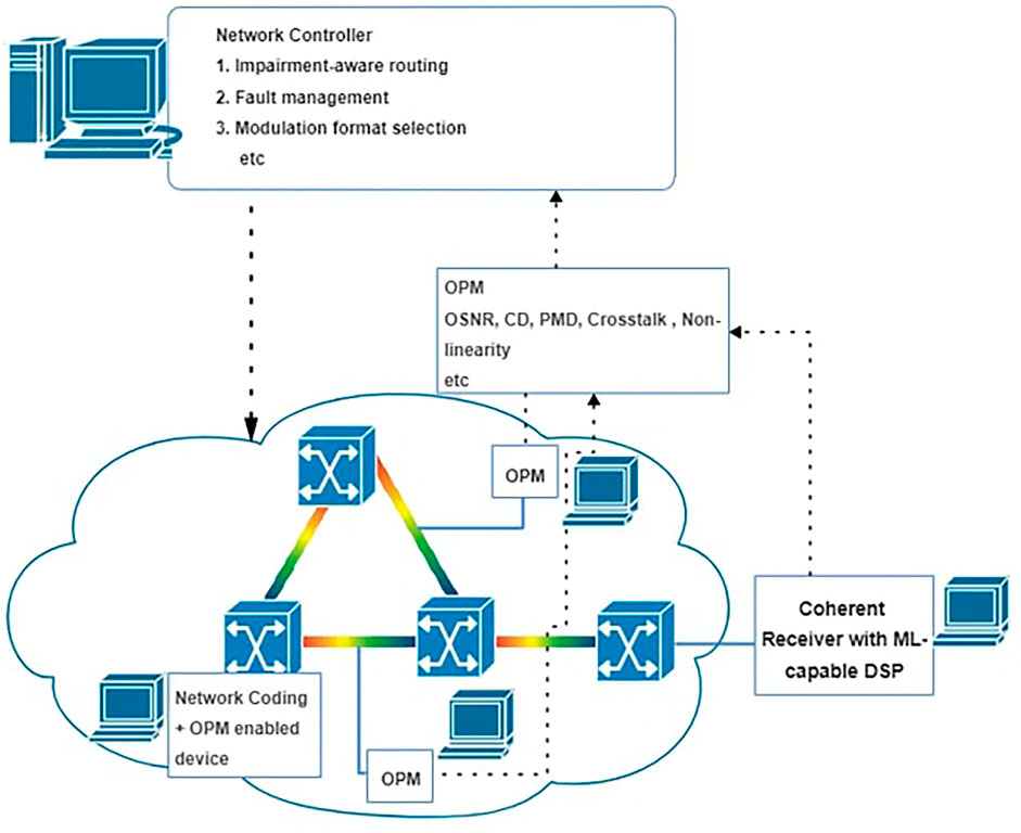
FIGURE 1. OPM enabled intelligent network diagram.
This paper aims to survey existing work where machine learning has been applied to aid in OPM and discuss the performance of the different techniques. Moreover, since the bulk of the techniques employed in the current literature require advance knowledge of the signal type, we also review some works that identify the modulation format and bitrate. Furthermore, we briefly explore work on photonic reservoir computing which has more recently been shown to be applicable to modulation format recognition.
2 Related Work
There are a number of review works on utilization of Machine Learning for various applications in optical networks. Existing and future technologies for OPM for both direct and coherent detection systems are reviewed in Dong et al. (2016), however, their work presented a broad range of techniques and did not focus on ML techniques. A detailed review of the different optical ML techniques was given in Mata et al. (2018), Khan et al. (2019b), and Musumeci et al. (2019) highlighting how they have been used in optical communications and networking functions such as for OPM, fault detection, non-linearity compensation and software defined networking. They, however, had limited coverage of OPM and Modulation Format Recognition (MFR). A detailed survey on OPM and MFR has been done in Saif et al. (2020). We update the current literature in this work as well as include the application of photonic reservoir computing which has only recently been applied to modulation format identification. The work in Amirabadi (2019) considered a detailed description of machine learning techniques and reviewed works that had applied them in the optical communications space.
3 Introduction to Machine Learning Algorithms
Machine learning can be generally viewed as either supervised, unsupervised or reinforcement learning. In supervised learning, there exists a dataset of labelled examples (xi, yi), i = 1…, M where xi are input variables or feature vectors that describe characteristics of the example and yi are the output variables (Burkov, 2019). The machine learning algorithm then aims to define a model to fit the data. It consists of either a regression problem or a classification problem. Regression predicts a continuous valued output function from the data whereas classification predicts discrete valued output. Once the model has been developed/trained, it can then be used to predict an output from unlabeled inputs. Unsupervised learning takes unlabeled data as input and finds structure or relationships among the data. Clustering algorithms group the data and return the cluster identity value for each example while other algorithms transform the data into other useful vectors or values.
3.1 Support Vector Machine
An SVM classifies data by viewing all data points as vectors in a high dimensional space and then deciding hyper-planes that separate the data into regions. The data is labelled as either positive or negative
3.2 K-Nearest Neighbors
In this method, all the labelled data examples are kept in memory after training. When a previously unseen example is encountered, it is compared to the existing data for example using euclidean distance and the k closest examples are determined. The predicted output is then the majority label or average depending on whether it is a classification or regression problem (Burkov, 2019).
3.3 Decision Tree
This algorithm classifies labelled data by evaluating the different features. If a particular feature being examined is below a certain threshold, the left branch is followed and right otherwise until a leaf node is arrived at which determines the class to which the data belongs (Burkov, 2019). Figure 2 shows these three ML algorithms.
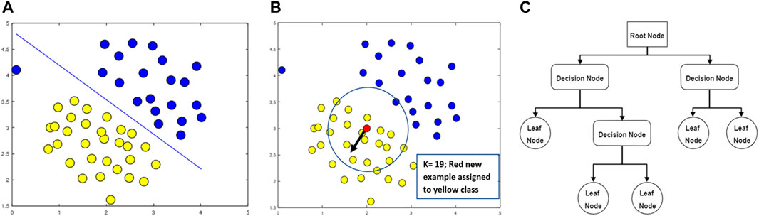
FIGURE 2. Illustration of different ML algorithms. (A) SVM, (B) K-nearest neighbors and (C) Decision Tree.
3.4 Artificial Neural Network
ANN’s are machine learning algorithms that try to imitate the human brain. The most common structure used in literature is a multiple layer perceptron which is made up of input and output layers and several hidden layers in between. Each hidden layer consists of one or more nodes known as neurons. The nodes in each layer are connected to each and every node in the subsequent layer and the connections characterized by parameters known as weights which define the strength of each connection. The weights are in the form of matrices which determine the mapping from one layer to another. Figure 3 shows one such ANN. The basic operation of each intermediate node is as follows; it receives a vector of input variables, transforms it linearly, applies an activation function and then passes the output to the nodes in the next layer and so on Burkov (2019). The goal of the ANN algorithm is to determine the weights that minimize the error between the predicted output values and the actual outputs. The ANN is presented with inputs and outputs and it learns the relationships between them through training. In the training phase, the weights are initialized to random values, and the output predicted. The predicted values are then compared to the actual output values and an error computed. Next, error derivatives are calculated and summed for each weight until the entire training dataset has been evaluated. The error derivatives are utilized to update the weights and the training is continued until an acceptable minimum error is obtained (Jargon et al., 2009b; Musumeci et al., 2019). This method of updating the weights is known as back propagation. Training a neural network can get computationally complex and time intensive as the hidden layers increase. Networks with multiple hidden layers are known as Deep Neural Networks (DNN’s). Several improvements have been made over time to optimize the training process for DNN’s such as Convolutional Neural Networks (CNN’s), Long Short Term Memory (LSTM) etc. For a more in depth description of these methods, the reader is referred to Hochreiter and Schmidhuber (1997), Gers et al. (1999), Cristianini and Shawe-Taylor (2000), and Burkov (2019).
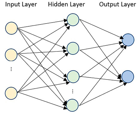
FIGURE 3. 3 layer ANN with a single input, hidden and output layer.
The algorithms discussed above are supervised learning algorithms. We shall briefly review two unsupervised learning algorithms that have been applied in OPM literature.
3.5 K-Means Clustering
This method takes unlabeled data and groups it into K clusters. It works by randomly initializing K centroids in the feature space and then assigning the data points to K clusters depending on which centroid they are closest to for example by calculating the Euclidean distance of each example from each of the K centroids. The data point is then assigned to the cluster whose centroid has the shortest distance to it. A new centroid is calculated by averaging all the examples in the cluster and the method repeated until the cluster assignments do not change anymore (Burkov, 2019).
3.6 Principal Component Analysis
PCA is a method used to reduce the dimension of the feature space. It works by computing eigen vectors called principal components which define the axes of the new feature space. The first axis is in the direction of the highest variance of the data, the second is perpendicular to it and in the direction of the second highest variance of the data and so on (Burkov, 2019). It is normally used in data compression.
4 Feature Selection for Optical Performance Monitoring
From the previous section, it can be seen that machine learning algorithms typically take input data features and learn relationships between them, thereby being able to group the inputs in a certain way or map the relationship to a function that can predict a required output. For OPM, the outputs are the type of impairment and its amount, while the inputs are signal representations. The signal representations are obtained from monitoring the signal waveform, polarization or spectrum (Dong et al., 2016) or from Digital Signal Processing (DSP) techniques in the electrical domain after detection in direct detection schemes. Coherent receivers already include powerful DSP blocks and input features can directly be obtained from the asynchronously sampled output of these blocks (Tanimura et al., 2016; Cho et al., 2019), or from constellation diagrams that can be constructed from them (Kashi et al., 2017; Wang et al., 2017).
The output of these various methods can then be utilized in the form of direct images or their properties, or statistical representations for example histograms, means, variances and moments to extract different features that can then be fed to the machine learning processing blocks. The features are chosen either manually by visual inspection or learnt by the ML algorithm and they show a clear distinction among different types of impairments and their levels. Table 1 shows a summary of monitored impairments for different feature types in current works.
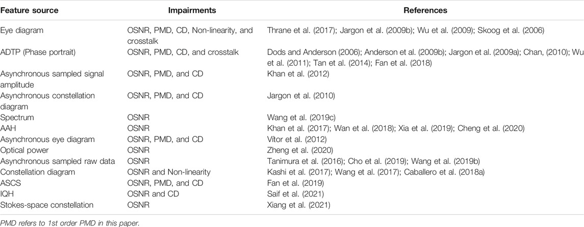
TABLE 1. Summary of features and monitored impairments used in current works.
4.1 Eye Diagrams
An eye diagram is a graphical representation of a signal waveform showing the amplitude distribution over one or more bit periods, with the symbols overlapping each other. The quality of the signal can then be determined from various characteristics of the eye opening for example jitter, SNR, dispersion, non-linearities.
Eye diagrams have been used in the current literature to monitor OSNR, PMD, CD, non-linearity, and crosstalk. Figure 4 shows the eye diagrams for an RZ signal subjected to different impairments (Wu et al., 2009). Visual inspection shows that different impairments and different levels of the same impairment produce distinct characteristics. These characteristics can be exploited by applying image processing techniques such as in Skoog et al. (2006), by defining statistical features from the sampled amplitudes for example means and variances at specific points on the eye diagram (Thrane et al., 2017), or by calculating the widely used parameters of the eye diagrams (Jargon et al., 2009b; Wu et al., 2009). Construction of eye diagrams is dependent on the modulation format and requires timing synchronization hence some form of clock recovery is required which can be expensive. An eye diagram also has no phase information about the signal.
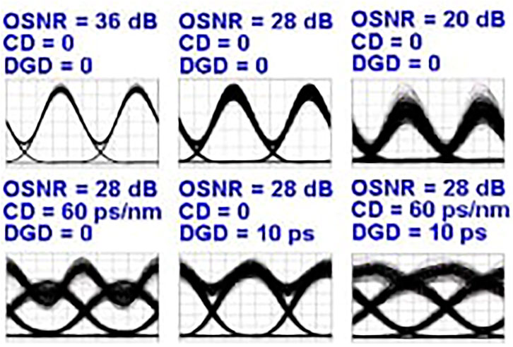
FIGURE 4. Impact of various impairments on the eye diagram of an RZ signal (Wu et al., 2009).
4.2 Asynchronous Delay Tap Plots
This technique also provides a visual representation of a signal known as a phase portrait. The signal waveform is split and one part of the signal delayed by a certain amount Δt. The signal and its delayed version are then sampled at the same instant and the pair of values (x,y) obtained plotted in a 2D histogram (Dods and Anderson, 2006; Chan, 2010). Figure 5 illustrates how a phase portrait is created from delay tap sample pairs (Anderson T. B. et al., 2009). The sampling period, Ts is independent of the bit duration, T and can therefore be several magnitudes larger. The portraits can be treated as images and exploited using pattern recognition (Anderson T. B. et al., 2009; Tan et al., 2014; Anderson T. et al., 2009) and then image processing algorithms applied, or specific features extracted from them for example the work in Jargon et al. (2009a) divided the phase portrait into quadrants and then defined statistical means and standard deviations of the (x,y) pairs and radial coordinates. Phase portraits are also dependent on the signal properties such as bitrate and modulation format and the tap delay. The tap delay is usually a certain fraction or multiple of the symbol rate and thus needs to be adjusted exactly for different datarates to allow accurate monitoring (Khan et al., 2011). ADTP’s have been used for multiple impairment monitoring of OSNR, CD, crosstalk and 1st order PMD. In Figure 6, the effect of various impairments on the ADTP of a 10 Gbps NRZ signal at two different delays, T and T/4, as well as the corresponding eye diagrams are shown (Chan, 2010).
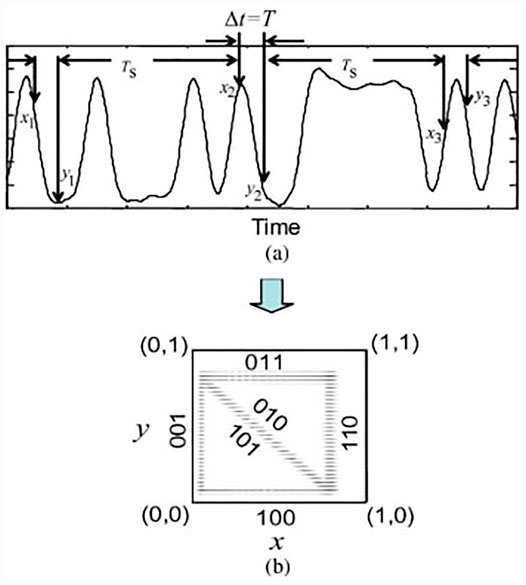
FIGURE 5. Generation of phase portrait (Anderson T. B. et al., 2009).
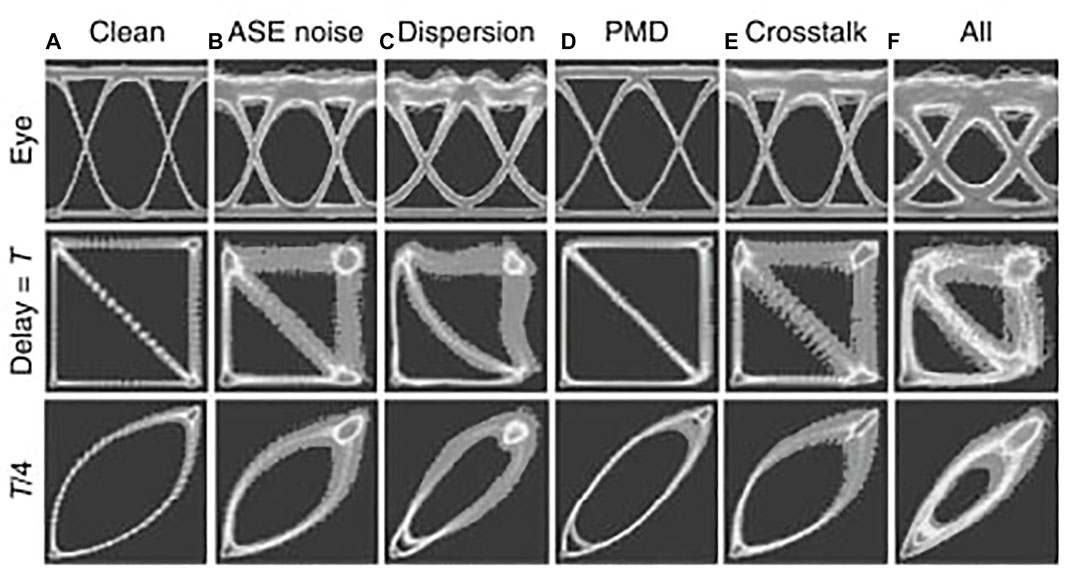
FIGURE 6. ADTP’s for a 10 Gb/s NRZ signal in the following scenarios: (A) OSNR = 35 dB, (B) OSNR = 25 dB, (C) CD = 800 ps/nm, (D) DGD = 40 ps, (E) crosstalk = −25 dB and (F) a combination of (B–F) (Chan, 2010).
4.3 Asynchronous Amplitude Histograms
AAH’s are obtained from random asynchronous sampling of the signal within the bit period. The authors in Chen et al. (2004) showed that with a sufficient number of samples, the amplitude distribution can be accurately represented within a bit period. The amplitude samples are arranged in bins corresponding to their level, and then the count of samples within each bin is plotted against the bin. This is in contrast to the synchronous AH where the considered samples are within a specific window for example 10% (Chan, 2010) of the bit period around the center of the eye diagram at the optimal decision time. The peaks in the AAH correspond to the samples around the maximum and minimum values of the eye, and the samples in between correspond to those around the crossings of the rising and falling edges of the waveform. Amplitude histograms are simple and transparent to the transmitted signal characteristics such as modulation format and bitrate, however, the contribution of each individual impairment cannot be independently extracted hence they have not been used for multiple impairment monitoring. Furthermore, the monitoring accuracy is dependent on the number of samples (Wan et al., 2018; Dong et al., 2016; Cheng et al., 2020). The count of occurrences at each bin can then be used as input features such as in Wan et al. (2018) and Khan et al. (2017). Xia et al. (2019) additionally used the variance of the amplitude values in each bin. Figure 7 shows results of varying the OSNR on the AAH for a 16-QAM signal (Khan et al., 2017).
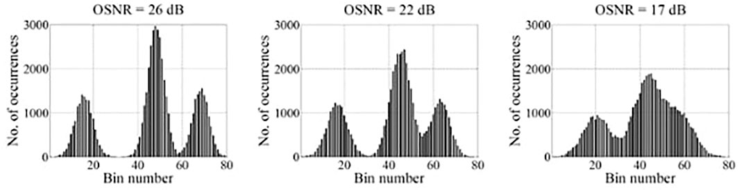
FIGURE 7. Impact of varying OSNR on the AH of a 16-QAM signal (Khan et al., 2017).
4.4 Asynchronous Single Channel Sampling
In this method, shown in Figure 8, the signal y(t) is sampled asynchronously using one tap, and then the samples are shifted by k samples and the sample pairs yi(t) and yi+k(t) used to construct a phase portrait. This method is less expensive than two-tap sampling (Yu et al., 2014; Fan et al., 2019; Fan et al., 2020). The generated phase portraits can be used as images for example in Fan et al. (2019) and Fan et al. (2020).
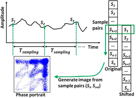
FIGURE 8. Generation of a phase portrait from ASCS (Fan et al., 2020).
4.5 Constellation Diagrams
A constellation diagram is a graphical representation of a digitally modulated signal, where received samples are represented in an I/Q diagram. They are used in coherent detection schemes and can be generated by techniques such as linear optical sampling (Dorrer et al., 2005). However, since coherent receivers already have embedded Digital Signal Processing (DSP) blocks, they can be directly constructed from the asynchronously sampled data output of the DSP. Thereafter, they can be used to generate manually defined features for example Caballero F. J. et al. (2018) defined tangential and normal components of the noise of each symbol and then used averages and amplitude noise covariances as inputs, or their images can be directly input the ML algorithm for image processing without the need for manual feature generation for example in Wang et al. (2017). Constellation diagrams have only been used to measure OSNR and non-linear noise in coherent detection system since the coherent receiver can already compensate for CD and PMD and therefore these impairments can be directly monitored.
4.6 In-Phase Quardrature Histograms
IQH’s were proposed in Saif et al. (2019) as an extension of AAH’s to include phase information for coherent systems. They contain similar information as constellation diagrams but with an additional representation of the amplitude in color. They showed that it can be used to identify OSNR, PMD and CD although performance degraded in the presence of multiple impairments. Figure 9 shows resulting IQH’s AH’s and constellation diagrams for different impairments. Saif et al. (2021) derived 1D features from projections of IQH’s on diagonal and horizontal axes.
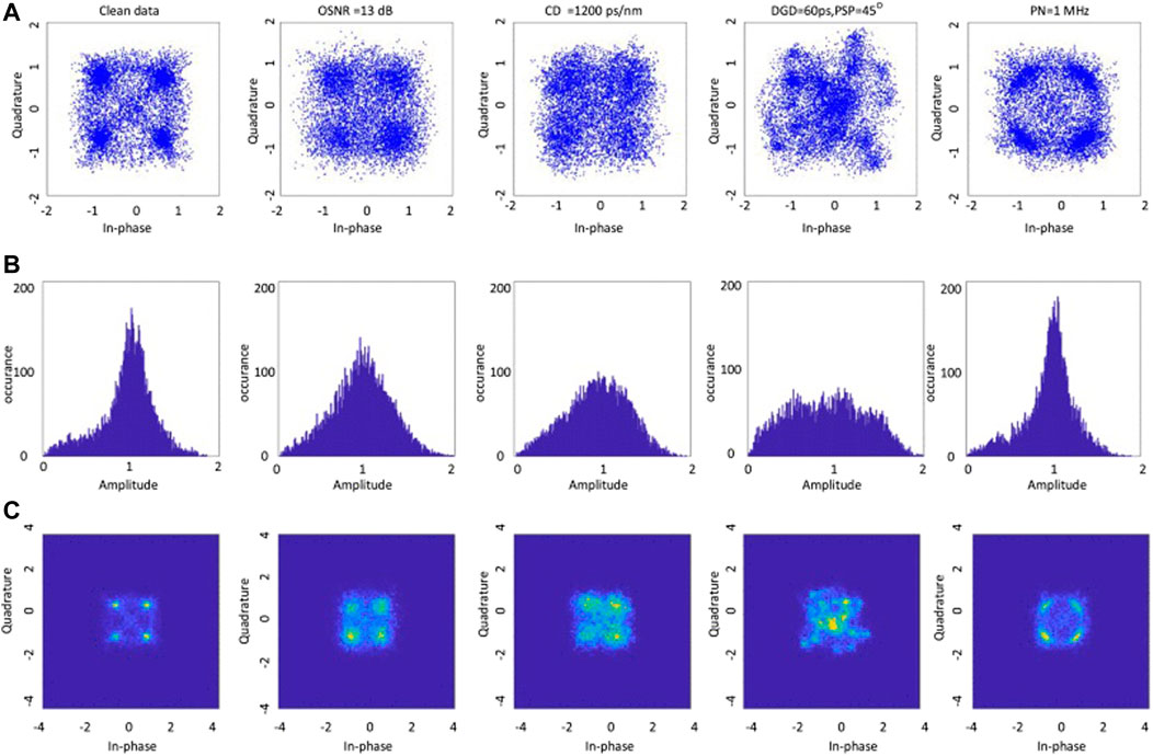
FIGURE 9. Comparison of constellation diagram, AAH and IQH (Saif et al., 2019).
4.7 Stokes Space Constellation
This diagram is obtained by plotting the last three components of the Stokes vector of the received complex signals from a coherent receiver in a 3D Stokes space. Different modulation formats present a specific number of distinguishable clusters in this space (Szafraniec et al., 2010; Boada et al., 2015; Mai et al., 2017). The authors in Xiang et al. (2021) obtained the cumulative distribution function (CDF) of one Stokes parameter while Zhang et al. (2020) projected the constellation onto three different 2D planes and used the resultant plots as images such as in Figure 10.
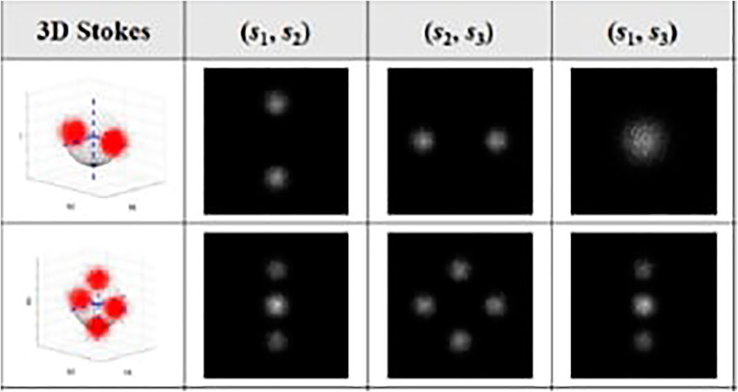
FIGURE 10. 3D Stokes constellation of a BPSK and QPSK signal, as well as their corresponding projections in the 2D Stokes planes at OSNR = 18 dB (Zhang et al., 2020).
4.8 Other Methods
The nature of asynchronous sampling means that certain information in the signal is lost, which could make it difficult in some cases to separate the effects of different impairments from the overall received signal in case they produce similar changes in the plots (Dods and Anderson, 2006). Furthermore, there is overlap in the distribution of signal amplitudes which makes it more challenging to extract individual distributions from AAH’s in practice (Khan et al., 2011). Asynchronous eye diagrams (Ribeiro et al., 2012) and asynchronous constellation diagrams (Jargon et al., 2010) can be constructed to mitigate this. In addition, Khan et al. (2011) also proposed asynchronously sampled amplitudes as a solution for better CD monitoring since previous works had shown that CD was severely impacted by changes in OSNR and Differential Group Delay and to eliminate the requirement for continuously adjusting the tap delay for multiple bitrates.
Optical spectral data from an optical spectrum analyzer (OSA) and optical power have also been used in Wang and Luo (2006) and Zheng et al. (2020), respectively.
5 Survey of Machine Learning-Based Optical Performance Monitoring Techniques
5.1 Optical Performance Monitoring for Networks Using Direct Detection
OPM modules in systems employing direct detection can be as straightforward as a photo-detector in combination with an Analog to Digital Converter.
Skoog et al. (2006) utilized multiple Support Vector Machines (SVM’s) to classify different impairments using images of eye diagrams, characterized by 23 low order zernike moments. Simulation data was used to train the model after impairments of CD, PMD and cross talk were applied. Four SVM’s were required, one for each impairment and an additional one for the normal case since they are binary classifiers. The number of input images used for training the model were 31, 107, 20 and 6 for CD, PMD, crosstalk and normal respectively. Experimental verification was then done using the model. Results collected from 3, 11 and 3 images for CD, PMD and crosstalk respectively showed that the method could classify the simulated and experimental data with accuracies of 95 and 60%. However, it could only identify the type of impairment but not the amount. Application of a nearest neighbors technique after the SVM was proposed to enable this.
In Jargon et al. (2009b), an Artificial Neural Network (ANN) consisting of a single hidden layer and 12 hidden neurons was demonstrated to predict multiple impairment levels simultaneously. The eye diagrams of signals with different bitrates and modulation formats i.e., 10 Gb/s non-return to zero on-off keying (NRZ-OOK) and 40 Gb/s return-to-zero differential phase shift keying (RZ-DPSK), to which different combinations of CD, PMD and OSNR had been applied, were used to train the ANN. 4 input features were extracted from each of 189 eye diagrams i.e. (Q-factor, closure, jitter and crossing amplitude/level of transition between adjacent zeros for NRZ-OOK/RZ-DPSK, respectively). 125 eye diagrams were used for training while 64 were used for validation. The ranges used for OSNR, CD and Differential Group Delay (DGD) were 16–32 dB, 0–800 ps/nm, and 0–40 ps for NRZ-OOK, and 16–32 dB, 0–60 ps/nm and 0–10 ps for RZ-DPSK. A correlation coefficient of 0.91 was achieved for the NRZ-OOK signals while 0.96 was found for the RZ-DPSK case. A similar investigation was done in later work in Jargon et al. (2009a), but using seven manually defined parameters from ADTP’s as input to a single layer, 28 neuron ANN for the 10 Gbps NRZ-OOK case. A higher correlation coefficient of 0.97 was obtained over similar impairment ranges. The work was further extended to monitor the same three impairments for a 40 Gbps RZ-QPSK signal and manually defined input parameters using asynchronous constellation diagrams (Jargon et al., 2010). An identical ANN was used in Jargon et al. (2009a) achieving a correlation coefficient of 0.987, and root mean square errors (RMSE’s) of 0.77 dB, 18.71 ps/nm and 1.17 ps for OSNR, CD and DGD respectively. The impairment ranges tested were 12–32 dB, 200 ps/nm and 0–20 ps for OSNR, CD and DGD. The same ANN technique with one hidden layer and 12 hidden neurons was used in (Wu et al., 2009) to monitor the effect of multiple impairments on 40 Gbps RZ-OOK and RZ-DPSK data signals. four input parameters (Q-factor, eye-closure, RMS jitter, and RMS jitter) were defined from eye diagrams. The ANN was trained and tested with data from both simulation and experiment. In the simulation, 125 and 64 eye diagrams were used for training and validation, respectively, achieving a correlation coefficient of 0.97 and 0.96 for OOK and DPSK, respectively and average errors for OSNR, CD and DGD of 0.57 dB, 4.68 ps/nm and 1.53 ps for OOK and 0.77 dB, 4.47 ps/nm and 0.92 ps for DPSK. The simulations were followed up with an experiment, in which 20 and 12 eye diagrams were used for training and testing respectively to estimate OSNR and CD. The results showed a better performance than simulation with 0.99 correlation coefficient for both signals. The average errors for OOK were 0.58 dB and 2.53 ps/nm while those for DPSK were 1.85 dB and 3.18 ps/nm. The ranges tested for OSNR, CD and DGD were 16–32 dB, 0–60 ps/nm and 1.25–8.75 ps. The authors then monitored the impact of accumulated fiber non-linearity in a 40 Gb/s RZ-DPSK Wavelength Division Multiplexed (WDM) system consisting of 3-channels using a simulation in which additional features consisting of statistics of the 1 and 0 values were defined giving a total of 8 inputs. The input optical power was varied from −5 to 3 dB m, while OSNR, CD and DGD were tested over the ranges from 20 to 36 dB, 0–40 ps/nm and 0–8 ps. Equally good results were obtained: correlation coefficient of 0.97, and mean error of 0.46 dB, 1.45 dB, 3.98 ps/nm and 0.65 ps for optical power, OSNR, CD, and DGD from 135 training samples and 32 testing samples.
Anderson et al. (2009b) simultaneously measured CD and DGD for a 40 Gb/s NRZ-DPSK signal. ADTP’s were generated and then kernel based ridge regression applied to predict the impairments using 900 features. Simulation was done for various combinations of CD, DGD and OSNR ranging from 0 to 700 ps/nm, 0–20 ps and 13–26 dB, respectively. 1,200 phase portraits consisting of 900 features each were used for training, and independent training for a single impairment in the presence of all other impurity ranges was done. 500 phase portraits were used for verification. RMSE’s of ±11 ps/nm and ±0.75 ps for CD and DGD respectively were achieved. Experimental verification was also done using a split of 1,500:500 phase portraits for training: validation for OSNR, CD and DGD ranging from 15 to 25 dB, −400 to 400 ps/nm and 0–22.5 ps. The total training time was 3 h and RMSE of ±11 ps/nm and ±1.9 ps for CD and DGD obtained. Prior knowledge of modulation and bit rate was assumed.
OSNR, PMD and the magnitude and sign of CD were monitored in Khan et al. (2012) using an ANN whose input features were derived from the empirical moments of amplitude samples. The ANN consisted of a single hidden layer with 42 neurons and was trained with simulation data for 56 Gb/s RZ-DQPSK and 40 Gb/s RZ-DQPSK and DPSK signals. For each datarate-modulation format combination, 3,627 groups of moments were collected over varying ranges of OSNR (10–26 dB), CD (−500 to 500 ps/nm) and DGD (0–14 ps). A root mean square errors of 0.1 dB was obtained for OSNR in all three cases while the values obtained for CD and DGD were CD (27.3, 29, 17 ps/nm) and DGD (0.94, 1.3, 1 ps) for 40 Gb/s RZ-DQPSK, 56 Gb/s RZ-DQPSK and 40 Gb/s RZ-DPSK systems, respectively. The authors proposed increasing the number of moments to improve the results. Table 2 summarizes existing works for direct detection systems.
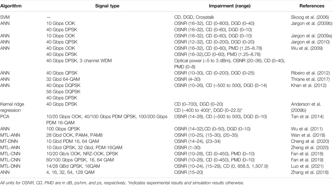
TABLE 2. Summary of existing OPM works for direct detection.
The work presented in Tan et al. (2014) monitored multiple impairments and identified both modulation format and bit rate using Principal Component Analysis (PCA). Input features were derived from images of ADTP’s and the method was shown to be suitable for heterogeneous networks. Simulations were used to generate 26,208 ADTP’s from different combinations of impairments, modulation schemes and bitrate. Previous methods seen so far have assumed knowledge of both bitrate and modulation. The impairments were varied in the range 14–28 dB (OSNR), −500 to 500 ps/nm (CD) and 0–10 ps (DGD). The signal combinations used were 10 and 20 Gb/s RZ-OOK, 40 and 100 Gb/s PDM RZ-QPSK and 100/200 Gb/s PDM NRZ 16-QAM. The results showed an overall mean estimation error of 1 dB (OSNR), 4 ps/nm (CD) and 1.6 ps (DGD). The performance of the method under fiber non linearity was also investigated and found to be slightly less accurate, increasing the mean errors to 1.2 dB for OSNR, 12 ps/nm for CD and 2.1 ps for DGD. To mitigate this, selection of additional features to characterize different non-linearity coefficients and link/span lengths was proposed. In this way CD, OSNR and DGD could be monitored without advance knowledge of the signal type, it was part of the training data.
The authors in Thrane et al. (2017) used an ANN for in-band OSNR monitoring on 32 Gbaud directly detected PDM-QAM signals. The input features were selected from eye diagrams. In addition to the modulation format, this method required knowledge of the pulse shape therefore it was necessary to train a separate neural network for each pulse-MF pair. It was composed of one hidden layer, three hidden neurons and only one input feature i.e. the variance at the maximum amplitude points on the eye diagram. Experimental verification was done for OSNR’s in the range of 4–30 dB but only in white Gaussian noise. The results showed that OSNR estimation was accurate between 4–17 dB with a mean error of 0.2 dB but worsened from 17 to 30 dB. This was attributed to the fact that eye diagrams at higher OSNR’s did not vary very significantly and hence had less distinguishable features. Since real transmission channels face other impairments, simulation was done for chromatic dispersion (CD) and the method found to be unimpaired up to 250 km on a dispersion uncompensated link. Verification of the method in the presence of other effects was left to future work.
Multi-impairment monitoring was investigated in Wu et al. (2011) using a single layer, 12 hidden neuron ANN that was trained with simulated data from 180 ADTP’s. Seven statistical features were extracted from each ADTP obtained from sampling a 100 Gb/s QPSK signal over impairment ranges of OSNR (14–32 dB), CD (0–50 ps/nm) and DGD (0–10 ps), respectively. The validation was done with 144 samples. Balanced detection was shown to perform better than single ended detection through simulation with correlation coefficients of 0.995 and 0.96, respectively. The RMSE’s were obtained as OSNR (1.62/0.45 dB), CD (8.75/3.67 ps/nm) and DGD (7.02/0.8 ps) for single/balanced detection. Experimental data was used to validate the performance for balanced detection and produced correlation of 0.997.
Simultaneous monitoring of PMD, CD, and OSNR using a single layer, 40 neuron ANN was shown in Ribeiro et al. (2012) used a single hidden layer ANN with 40 neurons. Parametric asynchronous eye diagrams (PAED’s) of a 40 Gbps QPSK signal were collected, from which 24 statistical position features were extracted. In this work, RMSE’s of <20 ps/nm, <1.3 ps, and 1.5–2 dB were found via simulation for impairments in the ranges 0–200 ps/nm, 0–25 ps and 0–30 dB.
In Wan et al. (2018) a Multi Task Learning ANN (MTL-ANN) was investigated using features extracted from amplitude histograms and used to acquire both OSNR and the modulation format. Simulations were done on 28-Gbaud NRZ-OOK, PAM4 and PAM8 over an OSNR range of 10–25 dB, 15–30 dB and 20–35 dB, respectively and CD range of −100 to 100 ps/nm. A total 9,072 and 1,008 simulated AH’s were used for training and testing respectively. Different combinations of OSNR and modulation format at specific CD values were tested achieving a MSE of 0.12 dB. Experimental verification was done for OSNR ranges of 14–29, 17–32 and 22–37 dB for OOK, PAM, PAM8 and datasets consisting of 4,320 and 480 AH’s for training and testing. The results showed higher accuracy than single task learning ANNS (STL-ANN’s), achieving MSE of 0.11 dB compared to 0.4 dB for a STL-ANN with a similar structure. This method required optimization of the bin number. Fewer bins were shown to have less accuracy while more bins led to a more complex ML structure. The authors used an optimal number of 100 in this work.
OSNR and modulation format monitoring was done in Cheng et al. (2020) using a mutli-task deep neural network with transfer learning (DNN-TL) using AH’s as inputs. The DNN was trained with 400 AH’s generated from simulation and then experimental verification for PDM-16 and 64-QAM, 10 Gbaud signals was done and the results achieved RMSE of 1.09 dB for OSNR ranging between 14 and 24 dB for PDM-16 QAM and 23–34 dB for 64-QAM, respectively. The ANN structure had 4 hidden layers with 100/50/30/2 neurons respectively. Application of transfer learning was able to reduce the required training samples from 322 to 243 (243) for the same RMSE.
A modulation format independent method was proposed to monitor the OSNR for a WDM system in Zheng et al. (2020). Optical power measured at different center wavelengths was used as input features to a MTL-ANN with 64 neurons per layer. Five samples for each OSNR (1–30 dB) were collected and a ratio of 70:30 samples was used for training: testing and shown experimentally to estimate the OSNR with a Mean Absolute Error (MAE) of 0.28 dB and RMSE of 0.48 dB for both the 10 Gbaud NRZ-QPSK and 32 baud PDM-16QAM over an OSNR range of 1–30 dB. It was also shown to be insensitive to CD and PMD. The same ANN was shown to be capable of simultaneously monitoring baud rate and launch power without deploying two additional ANN’s. For launch power in the range of 0–8 dBm, MAE and RMSE were 0.034 and 0.066 dB, respectively.
A MTL-CNN was used in Fan et al. (2018) to do multiple impairment monitoring in combination with joint bit rate and modulation format identification. 6,600 Phase portraits were generated from simulations of six different signal types i.e., 10/20 Gb/s RZ-OOK, NRZ OOK and NRZ-DPSK and impairments varied over the ranges 10–28 dB, 0–10 ps and 0–450 ps/nm for OSNR, DGD and CD, respectively. 90% of the images were used to train the CNN while 10% were reserved for testing. The results showed RMSE’s of 0.73 dB, 1.34 ps/nm, and 0.47 ps. The same authors improved their method by using phase portraits from ASCS in Fan et al. (2019) and features from the various CNN layers as opposed to only those in the last layer. In this method, the features were extracted from all the layers and transformed into the same space and then multiple tasks were trained for each of OPM, MFR and bitrate identification (BRI). 60/100 Gb/s signals for three modulation formats QPSK, 16 and 64-QAM were generated by simulation and the same impairment ranges and number of phase portraits were used. RMS errors of 1.52 ps/nm, 0.81 dB, and 0.32 ps were obtained.
In the work presented in Luo et al. (2021), adaptive ADTP’s and AAH’s were used as multiple inputs to a multi-task DNN to monitor OSNR in the range 10–24 dB and 15–29 dB for QPSK and 16 QAM signals respectively and identify the bitrate, modulation format and chromatic dispersion. 2 baudrates (14/28) and three values of CD (0, 858.5, and 1,507.9 ps/nm) were experimentally tested. In the AADTP, a single ADC is used to sample the data generating xm, samples (m > = 1) as opposed to two tap delay sampling and then a fixed time delay is introduced by setting the second sample pair as a ym = xm + n, n > = 1. The same samples are used to generate AAH’s. 36,000 AADTP’s and AAH’s were generated and 28,800 of them used to train the DNN. The method achieved a MAE of 0.2867 dB and CD identification accuracy of 99.83%.
A simple three layer ANN was used in Zhang et al. (2018)to jointly monitor OSNR (15–20 dB) and identify the MF in an IM-DD QAM-OFDM system. Two ANN’s were used; one for MFI and then once the MF was known, passed to the second ANN which was trained for each modulation format separately to identify the OSNR. AAH’s were derived from the IQ output by considering either the I or Q samples of 4, 16, 32, 64 and 128 QAM signals. To improve the OSNR accuracy at low OSNR’s, 5 distinct features were calculated from the AH’s and used as input to the second ANN i.e. mean, variance, range, interquartile and median. The errors obtained OSNR prediction were
Table 3 shows the performance of the different techniques that have been surveyed.
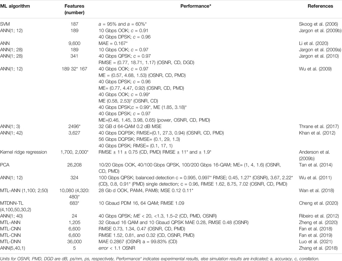
TABLE 3. Performance comparison of existing OPM works for direct detection.
5.2 Machine Learning Applied to Coherent Detection Systems
Coherent detectors already incorporate impairment compensation techniques at the receiver and therefore linear impairments—CD and PMD can be monitored. OSNR then becomes the key impairment that still requires monitoring. Many of the previous methods discussed required the careful selection of features from sampled data. These features varied for different system parameters. As networks evolve, they will transmit data at varying bitrates and modulation formats which may change randomly hence more advanced techniques are required.
The authors in Tanimura et al. (2016) used experimental data to train a Deep Neural Network (DNN) to monitor OSNR of a 16 GB d DP-QPSK signal with asynchronously sampled raw data from a coherent receiver. The DNN was trained with three different hidden layer structures (1, 3, 5) each comprising 512 neurons, and three training sample sizes (4,000, 40,000 and 400,000). The four tributary output from the coherent receiver was then fed to the DNN, each tributary containing 512 samples generated from experiment. The five layer, 400,000 case was selected as the best case. The trained DNN was then used to test 10,000 samples resulting in an average error of 1.6 dB over an OSNR range of 7.5–31 dB.
In Cho et al. (2019), the same method was extended to a Convolutional Neural Network (CNN) which was trained with experimental data containing 1,000,000 samples from 14 to 16 GBd DP-QPSK, 16-QAM and 64-QAM signals that had been subjected to different OSNR’s within a range of 11–33 dB. The CNN was validated using 10,000 test samples for each modulation format. The results obtained showed a bias error of less than 0.3 dB, however the training phase took several hours. They showed the method to be insensitive to CD and left non-linearity to future work.
A single layer ANN with six hidden neurons was used in Kashi et al. (2017) to estimate non-linear noise present in a 56.8 GB d DP 16-QAM signal transmitted over fiber channels with varying characteristics for example transmission distances, optical power, number of channels, types of fiber etc. The ANN was provided with the link parameters as well as amplitude noise co-variance (ANC) of the input symbols resulting from fiber non-linearity for 240 simulated cases. 70% of the samples were used for training and 30% for testing resulting in the errors obtained in the OSNR being less than 0.6 dB for two experimental cases.
In Caballero et al. (2018b) a neural network was used to estimate both linear and non-linear noise simultaneously using input features derived from constellation plots and the amplitude noise co-variance. The ANN consisted of one hidden layer and seven neurons and was trained with a 35 Gbd DP-16 QAM signal transmitted over different WDM channels, with varying fiber types and lengths of 320–1,200 km, launch power of −2.5 to 0.5 dBm and different applied Amplified Stimulated Emission (ASE) to non-linear noise ratios. The total samples were 2,160. Simulations and experimental data for varying optical power in an 800 km link were used and produced results with a std error of 0.23 dB.
In Wang et al. (2019b), a Long Short-Term Memory (LSTM) neural network was used to approximate the OSNR without need for manual feature extraction. The four tributary output from the coherent receiver was used as input. The LSTM-NN was trained from simulation of 28/35 GBd PDM 16 and 64-QAM signals and OSNR varied between 15–30 dB. 512 data samples were collected for each OSNR value for a total of 32,768 samples with 70% used for training and the rest for testing. The Mean Absolute Error (MAE) was found to be 0.1, 0.04, 0.05, and 0.04 dB for 28 GBd PDM 16 and 64-QAM and 35 GBd PDM 16 and 64-QAM respectively. The accuracy of the method was shown to be unaffected by linear impairments of CD and PMD through simulation with variable fiber length. Experimental verification of the model was done on a 34.94 GBd PDM 16-QAM signal with 5,632 samples over an OSNR range of 15–25 dB, resulting into a MAE of 0.05 dB.
The work in Khan et al. (2017) used a DNN to simultaneously identify modulation format and monitor OSNR. One DNN consisting of two hidden layers (45 and 10 neurons, respectively) determined the modulation format and then the result was passed to a second stage with multiple 2-hidden layer DNN’s (45/40 and 10 neurons respectively) trained per modulation format and the second DNN selected based on 1st stage results. The OSNR could then be predicted for different modulation formats. The input features were obtained from amplitude histograms of varying combinations of modulation formats and OSNR’s. 133 experimentally generated AH’s for different combinations of modulation format and OSNR were used to train the DNN’s and then tested on 57 AH’s for 112 Gb/s PDM QPSK, 112 Gb/s PDM 16-QAM, and 240 Gb/s PDM 64-QAM signals resulting in mean errors of 1.2, 0.4 and 1 dB respectively. This method however was shown to take significant training time and computational power. The same technique was employed in Li et al. (2020) for multiple QAM formats with an added anomaly detector between the MFI ANN and OSNR monitor to improve accuracy. 9,600 AH’s of 100 bins each were generated for 12.5 GBd signals and 6 modulation formats. The OSNR was varied over the ranges (10–25) for QPSK and 6-QAM, (15–30) for 16-QAM and (20–35) for 16, 48 and 64-QAM. Experimental results showed a MAE of 0.167 dB.
The authors in Wang et al. (2017) used a CNN to estimate OSNR and recognize modulation format using as input images of constellation diagrams. Simulations were done for 6 modulation techniques i.e., QPSK, 8PSK, 8-QAM, 16-QAM and 32-QAM over OSNR ranges of 15–30 dB and 64-QAM in the OSNR range of 20–35 dB. Experiments were carried out for 2-QPSK and 16-QAM. CD was also varied between −100 and 100 ps/nm. The training set consisted of 9,600 constellations. The simulation results showed >95% accuracy for 64-QAM and >99% accuracy for other formats. They also compared 4 other commonly used algorithms; decision tree with 100 splits, SVM, k-nearest neighbors with 10 neighbors, and BP-ANN with 50 hidden neurons, and found that the CNN achieved better results than the rest at the expense of some computational complexity and large training time. Similar to other methods using constellation diagrams, it performed better for low SNRS <21 dB. Experimental verification was done for QPSK and 16-QAM signals, testing with 20 constellations and results showed maximum error of 0.6 and 0.7 dB, respectively.
In Xia et al. (2019), a DNN with transfer learning was studied to monitor OSNR on 56 Gb/s QPSK signals. AH’s of the signals were used as input features and trained over an SNR range of 5–35 dB. Each sample AH consisted of 80 bins and the variances were also considered for a total of 81 features per sample. Physical layer parameters were also varied for example launch power (6–8 dB), dispersion (0–600 ps/nm) and bitrates (28–56 Gb/s). The ANN with 5-hidden layer structure bearing 64, 32, 16, 8 and 4 neurons, respectively was trained with simulated data and then tested with 128,000 experimentally generated samples, achieving a RMSE of <0.1 dB.
In Wang et al. (2019c), four different algorithms were applied to spectral data from a 20 Gbps QPSK signal i.e., SVM, ANN with 1 hidden layer and 100 hidden neurons, k nearest neighbors with 10 neighbors and decision tree with 20 splits in a coherent system to estimate OSNR. Training was done with 30 spectra consisting of 4,096 samples each collected over an OSNR range between 15–30 dB and the ratio of training:testing data was 2:1. Experimental verification using the same amount of data found that the SVM performed better for the test parameters and took the least computation time. Estimation accuracy was found to be 100, 100, 73.124, and 65.625 for SVM, k-nearest neighbors decision tree and ANN respectively. The poor performance of the ANN was attributed to a large number of input neurons (4,096) hence making it prone to under fitting due to increased model complexity. The testing time was also checked and the SVM and KNN found to take the least and longest time, respectively.
A binary CNN in which the activation weights were constrained to ±1 as opposed to floating values was used in Zhao et al. (2020) to predict OSNR for 9 different 12.5 GBd M-ary QAM signals. Experimental data consisting of gray-scale images of ring constellation diagrams were used. The total dataset consisted of 14,400 images, 100 images per modulation format for each of the 16 OSNR values. With OSNR ranging from 10–35 dB, and average accuracy of 98.91% was found, and was shown to be slightly less accurate than a floating CNN (99.95%) and similar to a multi-layer perceptron (98.86%) of similar structure, however with reduced energy and execution time.
In Yu et al. (2019), the authors used a MTL-ANN to do OSNR estimation and MFI identification similar to their earlier work in Wan et al. (2018), but applied to a coherent receiver and 9 M-QAM formats at 12.5 GBd. Experimentally generated ring constellation diagrams were transformed to AH’s consisting of 200 bins each and used as input features. They were generated over an OSNR range of 10–25 dB for QPSK, 6, 8 and 12-QAM, 15–30 dB for 16 and 24-QAM and 20–35 dB for 32, 48, and 64-QAM. 100 AH’s were generated per OSNR value and modulation format for a total dataset of 14,400 split into a training:test set of 90:10. The ANN consisted of one input layer with 200 neurons, and two specific hidden layers for OSNR, while one specific hidden layer was used for MFI, consisting of half the neurons in the previous layer. The optimal neuron number for the shared hidden layer was found to be 350. Results showed 98.7% accuracy and RMSE of 0.68 dB when using regression and classification, respectively.
A method to simultaneously monitor impairments independent of the signal type was shown in Wang et al. (2019a). An LSTM-NN(160,128,2) was used to predict CD (1,360–2040 ps/nm) and OSNR (15–30 dB) for 28/35 GBd PDM 16/64 QAM signals, using as input the 4 tributary output of the coherent receiver. 512 data samples are generated by simulation for different MF, BR, OSNR, and CD and 70% used for training. The prediction performance obtained was MAE of <0.1 dB and 0.64 ps/nm, respectively.
In Wang et al. (2020), an ANN was shown to estimate OSNR using eigen values consisting of 2nd and 4th order moments and various OSNR’s extracted from the rings of the constellation diagrams as input features. The system was then simulated with 112 Gb/s QPSK, 16 QAM and 120 Gb/s 64-QAM signals and OSNR ranges of 15–26, 19–29 and 22–31 dB, respectively. The number of input features for each of the modulation schemes is 3, 3, 9 and the hidden neurons are 5, 5, 12. RMSE’s of 0.17, 0.3, 0.68 dB were obtained. Experimental results produced RMSE’s of 0.46 and 0.65 for 10/20 Gbd QPSK/16-QAM generated in OSNR ranges of 13–26 and 20–30 dB.
The authors in Feng et al. (2020) use a MTL-CNN to experimentally estimate OSNR and identify MF for 28 GBd PDM 8, 16, 32, 64 QAM and 8-PSK and QPSK signals resulting in mean errors of 0.26, 0.4, 0.85, 0.64, 0.17, and 0.19, respectively. A total of 30,600 images of intensity density and differential phase density at different OSNR ranges QPSK (10–30), 8PSK, 8, 16 QAM (12–30), 32 QAM (17–33), 64 QAM (18–33) are used as input features and 85% used for training.
The authors in Ye et al. (2021) monitored OSNR using an LSTM-NN but considered the prediction as a classification problem by defining the continuous OSNR range (15–24 dB) into discrete 1 dB intervals. The NN consisted of 8, 48, 64, 10 neurons for the input, memory, hidden and output layers respectively and the dataset size was 3,000 generated from the IQ output of the coherent receiver, with 75% of the samples used for training. Simulation was done on a 30 GBd PDM 16 QAM signal resulting in standard deviation within 0.4 dB while experimental verification on a 20 GBd DP-QPSK signal resulted in a standard deviation within 0.67 dB.
OPM for few mode fibers was considered in Saif et al. (2021). In this work, OSNR, CD and mode coupling were monitored with the aid of three ML algorithms i.e., SVM, random forest and CNN. The input features were obtained by considering 2D IQH’s and their 1D projections in different planes. 200 datasets were generated for each impairment value. In their simulation, the CNN showed the best performance and was then chosen to experimentally verify the accuracy of the proposed technique, resulting in coefficients of determination of 0.98, 0.92, and 0.91 for OSNR, CD and MC respectively. A 10 GBd DP-QPSK signal and ranges of 0–20 dB, 160–1,120 ps/nm were used for OSNR and CD, respectively, as well as different mode coupling coefficients.
A single ANN was applied in Xiang et al. (2019) to jointly monitor the MF and OSNR for a 28 GS/s PDM QPSK and 8, 16 and 64 QAM signals over the OSNR range of 10–16, 12–18,15–22 and 22–29 dB, respectively. Their ANN had 50 hidden neurons and took as input two statistical features derived from the amplitude of the signals i.e., kurtosis and variance. Simulation showed mean estimation errors for the OSNR to be 0.005, 0.2, 0.17, and 0.67 using a dataset size of 400 per OSNR and MF. Experimental verification over the ranges 10–17, 14–20, 17–25 dB for QPSK, 8 and 16 QAM showed mean errors 0.15, 0.41 and 0.49 dB when 15 hidden neurons are used. The method was extended in Xiang et al. (2021) but 50 bins of the cdf of one stokes parameter was selected as the input. With a dataset size of 200 per OSNR and MF, OSNR ranges 10–18 dB, 12–20 dB, 12–20 dB, 16–24 dB, and 22–28 dB for QPSK, 8PSK, 8,16, 64 QAM, and 60 hidden neurons, simulation produced mean square errors of 0.086, 0.125, 0.038, 0.17, and 0.40 dB. Experimental verification resulted in mean OSNR estimation error of 0.13, 0.29, and 0.41 dB for QPSK, 8PSK and 16QAM.
Table 4 summarizes the current work on OPM for coherent detection.
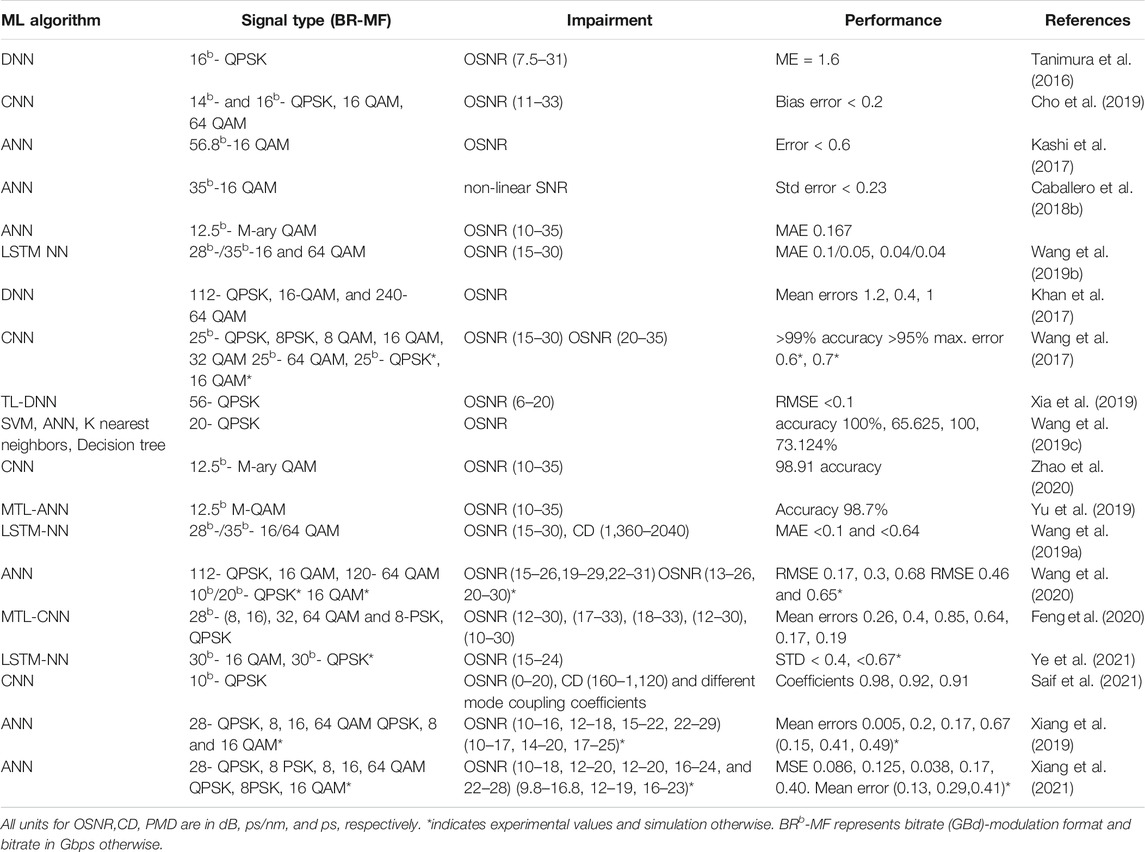
TABLE 4. Summary of existing OPM works-coherent detection.
5.3 Recognition of Modulation Format
Many of the OPM methods presented have assumed either advance knowledge of the modulation format or bitrate of the signal, or that it can be obtained from upper layer protocols. As a result, training of the ML algorithms and hence have been investigated for specific modulation formats and bit rates as seen in the previous section and would need to be retrained for a different signal type. It is also not practical to communicate across layers for simple OPM modules (Tan et al., 2014; Zhang et al., 2016) therefore it is necessary to review some works which have been done that have identified MFI and/or bitrate.
Since elastic optical networks utilize bandwidth variable transmitters, it would be useful for the OPM module to identify modulation format and bitrate. Tan et al. (2014) proposed one such method using Principal Component Analysis (PCA), where ADTP’s for different combinations of bit rate, modulation format and impairments (CD, PMD, and OSNR) were generated by simulation and PCA used to create a reference database for the training dataset, and then identified test data with 100% accuracy in the case when the PC’s
The work in Khan et al. (2017) utilized four DNN’s to identify OSNR and MF for three different signal types viz 112 Gbps PM QPSK and 16-QAM and 240 Gbps 64 QAM. One DNN was used to identify the modulation format, and the three DNN’s in the second stage trained to estimate the OSNR for one of the three modulation formats. Once the MF was identified, the signal was passed to the respective DNN in stage 2. The method was applied to experimental data from the output of a coherent receiver with AH’s used as input features. The method showed 100% accuracy in all three cases. The authors in Li et al. (2020) proposed an improvement to this method by adding an anomaly detector between the MFI identifier and OSNR monitor to ensure that the MF was accurately identified before being passed to the OSNR monitor. AH’s were constructed from constellation diagrams and the method experimentally verified for M-ary QAM. They achieved accuracies of 97.5%.
A MTL-ANN in conjuction with signal AH’s were applied for MFI and OSNR monitoring in Wan et al. (2018). Simulation and experiment for NRZ-OOK, PAM 8 and PAM 4 both yielded 100% accuracy for MFI. The authors extended their work in Yu et al. (2019) to 9 M-QAM modulation formats and used an adaptive weight loss ratio for their ANN as opposed to a fixed optimal one and also achieved 100% MFI identification accuracy. ANN’s and AAH’s were shown to correctly identify six commonly used modulation formats at several datarates and impairment levels with 99.6% accuracy in Zhang et al. (2016). Similarly, Huang et al. (2021) also used an ANN and AAH’s to identify the MF for NRZ, PAM4 and PAM8 signals under stringent bandwidth conditions. The results showed 95 and 100% accuracy for simulation and experiment.
Studies were done on the use of a Binary-CNN in Zhao et al. (2020) to identify the MF for 9 different M-ary QAM signals over different OSNR ranges. An experimentally generated data set consisting of 1,600 gray scale images of ring constellations per modulation format from the I/Q output of a coherent receiver, with a signal datarate of 12.5 GBd was used. The OSNR was varied from 10 to 35 dB and all the different formats were identified with 100% accuracy. This technique required less memory and execution time compared to a multi-layer perceptron and floating CNN.
In Zhang et al. (2020), MFI was done using a CNN that took as input 3 images generated mapping the IQ output from a coherent receiver onto a 3D stokes space, and then projecting it onto 3 2D stokes planes. Numerical simulations were done for 28 GBd PDM signals and 6 modulation formats (BPSK, QPSK, 8, 16, 32, and 64 QAM) in OSNR conditions varying from 9 to 35 dB. 68,400 and 16,200 images in total are used to train and test the CNN respectively. Results show identification accuracy of 99.96% when the OSNR is above 15 dB.
PCA was used in Xu et al. (2020) to identify the MF of 6 formats (BPSK, QPSK, 8, 16, 32 and 64 QAM). 3 PC’s were extracted from 2048 symbols of the stokes parameters from the received signals of a coherent receiver with OSNR varied from 8 to 40 dB and used as a reference database. Testing showed that 100% MFI accuracy could be obtained at minimum OSNR’s of 10, 8, 12, 18, 14 and 23 dB for BPSK, QPSK, 8, 16, 32 and 64 QAM PDM 28 GB d signals respectively. Experimental verification was also done on a dataset containing 30,720 symbols after construction of a reference from 2048 symbols for 20 GBd QPSK, 8, 16 and 32 QAM signals and also achieved 100% accuracy.
In Fan et al. (2018) MF and bit rate were determined by a MTL-CNN using 10/20 Gbps RZ-OOK, NRZ-DPSK and NRZ-OOK signals and phase portraits over various impairment ranges for OSNR, CD and PMD. Both MF and BR were identified with 100% accuracy. 100% accuracy was also attained by the same authors using a similar MTL-CNN structure but combining features from the different CNN layers and constructing phase portraits from ASCS (Fan et al., 2019).
A multi-input MTL-DNN was used to ascertain the modulation format and bitrate and simultaneously monitor OSNR and CD in Luo et al. (2021). An experiment was carried out over different OSNR ranges and three CD values using as input AADTPs and AAHs on 14/28 Gbd QPSK and 16QAM signals. MF and BR were identified with accuracy of 100 and 99.81%, respectively.
In Fan et al. (2018) MF and bit rate were identified by a MTL-CNN using 10/20 Gbps RZ-OOK, NRZ-DPSK and NRZ-OOK signals and phase portraits over various impairment ranges for OSNR, CD and PMD. Both MF and BR were identified with 100% accuracy. 100% accuracy was also attained by the same authors using a similar MTL-CNN structure but combining features from the different CNN layers and constructing phase portraits from ASCS (Fan et al., 2019).
A multi-input MTL-DNN was used to find modulation format and bitrate and simultaneously monitor OSNR and CD in Luo et al. (2021). An experiment was carried out over different OSNR ranges and three CD values using as input AADTPs and AAHs on 14/28 Gbd QPSK and 16QAM signals. MF and BR were identified with accuracy of 100 and 99.81%, respectively.
The authors in Zhang et al. (2018) used a 3-layer ANN(202,40,5) to identify 5 QAM formats in an experimental IM-DD QAM-OFDM system using AH’s as input. The MFI accuracy obtained was close to 100% for 4 and 16 QAM over the entire range of received optical power, while 32, 64 and 128 QAM got similar accuracy when the optical power exceeded −11 dBm.
In Feng et al. (2020) a MTL-CNN was shown to identify MF with 100% accuracy for mPSK and mQAM signals at a baud rate of 28 GBd and OSNR varied from 10 to 33dB.
A 3-layer ANN was also shown in Xiang et al. (2019), and Xiang et al. (2021) that achieved 100% MFI accuracy for different values of OSNR between 10–28 dB for 5 modulation formats.
The reviewed works on MFI are summarized in Table 5.
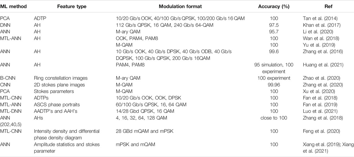
TABLE 5. Summary of ML methods used for MFI.
5.4 Application of Photonic Reservoir Computing in Optical Performance Monitoring
Photonic reservoir computing in the optical domain has been considered as an alternative to Digital Signal Processing for some years (Pachnicke and Li, 2020). A reservoir computer (RC) typically consists of an input, reservoir and readout. A input signal is fed to the reservoir, consisting of multiple randomly connected non-linear nodes, that function like a neural network. The input signal can alter the current and future states of the reservoir. The output of the reservoir is then readout as a linear combination of the different states in the reservoir. The input weights and node connections are fixed and thus the training complexity is reduced to a linear one at a single node at the readout (Vandoorne et al., 2008; Appeltant et al., 2011; Pachnicke and Li, 2020). A common implementation that has been presented in the literature uses a single non-linear element in combination with a delay loop (Appeltant et al., 2011), which can be implemented in the optical domain using a semiconductor laser and a fiber loop (Appeltant et al., 2011; Larger et al., 2012; Brunner et al., 2013). Other approaches have used a network of several interconnected Semiconductor Optical Amplifiers (SOA’s) (Vandoorne et al., 2008; Vandoorne et al., 2011), and silicon micro-ring resonators (Mesaritakis et al., 2013). (Vandoorne et al., 2014) has also shown a RC implementation using a passive silicon chip where the non-linearity is transferred to the readout, whose output is then passed to a linear classifier. Implementing the RC using photonic devices brings several advantages such as speed due to their inherently parallel computation nature, low power consumption and high bandwidth operation which are direct results of using light rather than electrical signals (Larger et al., 2012; Vandoorne et al., 2014). The authors in Cai et al. (2021) have applied this concept of reservoir computing using a semiconductor laser and delay line to identify the modulation format of 10 Gb/s OOK, 40 Gb/s DQPSK and 100 Gb/s 16-QAM signals in varying OSNR (12–26 dB), CD (−500 to 500 ps/nm) and DGD (0–20 ps) conditions. The input features were derived from AAH’s. From a dataset size of 11,700, 2,700 modulation signals were used to train the model using ridge regression and 100 samples used for testing. The training and testing process is repeated five times with the different sample sets and using 400 virtual nodes. The method achieved a classification accuracy of 95.1, 95.7 and 95.5% for OOK, DPQSK and 16-QAM.
6 Discussion
The most common features used in the current OPM works for feature selection are eye diagrams, phase portraits and amplitude histograms. In some cases, widely known features from these plots such as statistical means, variances, standard deviations etc, counts of occurrences per bin, eye diagram parameters like eye closure, crossing amplitude etc. have been used, while in others new features have been defined to exploit visible differences in the plots (Jargon et al., 2009a; Caballero F. J. et al., 2018; Saif et al., 2021). Manual definition of features is a difficult task which requires experience and also makes it impossible to distinguish patterns when there are only slight differences for example, the performance of ANN’s have been shown to deteriorate beyond certain OSNR’s because there is very little distinction between the eye diagrams especially for higher modulation formats (Thrane et al., 2017). It also makes it difficult to scale the ML algorithm to a different signal type than what it was trained with. To mitigate this, deep learning techniques have been studied where the algorithm can learn its own features from the input data, the commonest way being by supplying it with processed images (Wang et al., 2017; Fan et al., 2019; Fan et al., 2020; Zhang et al., 2020) and the 4-tributary output of the coherent receiver. Of course, this comes with more complexity since deep learning algorithms are generally more difficult to train. Furthermore, in cases where images are used, some amount of image processing is required (Skoog et al., 2006; Zhang et al., 2020).
Artificial neural networks have been very widely used for OPM in direct detection systems. The reviewed works have shown that in some cases, even simple ANN’s with one hidden layer and as low as three hidden neurons and as few as one input feature are capable of accurately predicting OSNR, CD, and PMD. Correlations of upto 0.997 have been obtained. The performance of the ANN depends on the input features selected and their number and also on the signal type. SVMs, PCA and ridge regression have also been used for but in very limited works. Deep learning techniques have also been shown in the literature but require significant time and more features to accurately train.
Many of the techniques used are dependent on the signal type hence it is assumed that the monitoring unit already has knowledge of the signal type. Moreover, in the cases where multi-impairment monitoring is required of different signal types, the ANN has to be trained more than once or multiple ANN’s have to be used for each signal type. Tan et al. (2014) proposed a method using PCA and that was transparent to the BR and MF but required training with multiple combinations of MF-BR-impairments hence required a significant amount of training data. More recently, Zheng et al. (2020) has shown a method which is transparent to the signal type and only requires input power as a feature. However, it has only been used to measure OSNR. Other works have also utilized multi-task learning and deep learning (Fan et al., 2018; Wan et al., 2018; Cheng et al., 2020) to simultaneously identify the signal type and impairments. These also required generating large training datasets with different combinations of the signal type and impairment levels. Very few works have measured other impairments such as non-linearity whose monitoring is also crucial for optical networks.
For coherent detection systems, neural networks have been used and shown to perform better than other methods where there have been compared except in one case in Wang D. et al. (2019). ANN’s still suffer from manual feature generation and as such most of the literature uses DNN’s and CNN’s for coherent detection systems which can learn their own features from the 4 tributary output of the coherent receiver, images of constellations in the Jones or Stokes space or AH’s. The challenge is that the training takes a considerable amount of time and a very large number of samples are required to produce accurate models. Nevertheless, after the training stage, the monitoring stage takes a shorter time, which is the critical time for an OPM monitor in a real system, since he training can be done off-line. Many of the methods have also been shown to maintain their accuracy in the presence of linear impairments. Zhao et al. (2020) tried to compare the performance of their joint MFI and SNR predictor by simulation for different transmission parameters noting that future networks will have varying parameters. They varied the transmission distance and launch power. They showed that if the DNN’s were trained each time there was a change in one parameter, 100% accuracy could be obtained for both MFI and OPM, whereas lower accuracy was obtained if trained once with a dataset consisting of all the possible parameter variations.
It is difficult to directly compare one ML implementation in one work over the other because different authors have carried out their simulations/experiments for different impairment ranges, signal types and they have classified the performance of their algorithms in different ways.
In the reviewed literature where MFR and BRI have been investigated, again ANN’s and deep learning neural networks have been the most common method of choice and the bulk of the work has achieved 100% identification accuracy.
Photonic reservoir computing is a promising technology for OPM and MFR since it reduces the training complexity of neural network based methods which has been highlighted as a key challenge in the reviewed works that have employed them. Moreover, signal processing in the optical domain allows for high speed and high bandwidth operation which are critical for future communication networks.
7 Conclusion
Optical performance monitoring has been an important aspect of optical communications for a very long time. As networks have become more heterogeneous and dynamic, they have also become more complex. Fiber network technology, which can already provide sufficient capacity, has had to evolve to meet the reliability demands. In addition to the light paths that will have to constantly change in order to provide bandwidth on demand, the signal parameters are also expected to be dynamic during transmission in accordance with link conditions. As a result, real time link performance has become important. Application of machine learning to Optical Performance Monitoring has garnered significant interest as a promising technology to aid in this task and has been shown to be possible, and to provide accurate prediction for multiple impairments as long as the algorithm is well trained.
Author Contributions
DT structured and wrote the first draft of the manuscript. AK and JS originated the idea of the review and edited the manuscript.
Conflict of Interest
The authors declare that the research was conducted in the absence of any commercial or financial relationships that could be construed as a potential conflict of interest.
Publisher’s Note
All claims expressed in this article are solely those of the authors and do not necessarily represent those of their affiliated organizations, or those of the publisher, the editors and the reviewers. Any product that may be evaluated in this article, or claim that may be made by its manufacturer, is not guaranteed or endorsed by the publisher.
References
Amirabadi, M. A. (2019). A Survey on Machine Learning for Optical Communication [machine Learning View]. arXiv
Anderson, T. B., Kowalczyk, A., Clarke, K., Dods, S. D., Hewitt, D., and Li, J. C. (2009b). Multi Impairment Monitoring for Optical Networks. J. Lightwave Technol. 27, 3729–3736. doi:10.1109/JLT.2009.2025052
Anderson, T., Clarke, K., Beaman, D., Ferra, H., Birk, M., Zhang, G., et al. (2009a). “Experimental Demonstration of Multi-Impairment Monitoring on a Commercial 10 Gbit/s Nrz Wdm Channel,” in Conference on Optical Fiber Communication, Technical Digest Series, San Diego, CA, March 22–26, 2009, 6–8. doi:10.1364/ofc.2009.othh7
Appeltant, L., Soriano, M. C., Van der Sande, G., Danckaert, J., Massar, S., Dambre, J., et al. (2011). Information Processing Using a Single Dynamical Node as Complex System. Nat. Commun. 2, 1–6. doi:10.1038/ncomms1476
Berthold, J., Saleh, A. A. M., Blair, L., and Simmons, J. M. (2008). Optical Networking: Past, Present, and Future. J. Lightwave Technol. 26, 1104–1118. doi:10.1109/JLT.2008.923609
Boada, R., Borkowski, R., and Monroy, I. T. (2015). Clustering Algorithms for Stokes Space Modulation Format Recognition. Opt. Express 23, 15521. doi:10.1364/oe.23.015521
Brunner, D., Soriano, M. C., Mirasso, C. R., and Fischer, I. (2013). Parallel Photonic Information Processing at Gigabyte Per Second Data Rates Using Transient States. Nat. Commun. 4, 1364. doi:10.1038/ncomms2368
Caballero, F. J., Ives, D., Zhuge, Q., O’Sullivan, M., and Savory, S. J. (2018a). “Joint Estimation of Linear and Non-linear Signal-To-Noise Ratio Based on Neural Networks,” in 2018 Optical Fiber Communications Conference and Exposition, OFC 2018-Proceedings, San Diego, CA, March 11–15, 2018, 1–3. doi:10.1364/ofc.2018.m2f.4
Caballero, F. J. V., Ivesc, D., Zbugec, Q., Sullivanc, M. O., and Savorfl, S. J. (2018b). “Joint Estimation of Linear and Non-Linear Signal-To-Noise Ratio Based on Neural Networks,” in (OSA) Optical Fiber Communication Conference 2018, San Diego, CA, March 11–15, 2018, 7–10. doi:10.1364/ofc.2018.m2f.4
Cai, Q., Guo, Y., Li, P., Bogris, A., Shore, A., Zhang, Y., et al. (2021). Modulation Format Identification in Fiber Communications Using Single Dynamical Node-Based Photonic Reservoir Computing. Photon. Res. 9, B1–B8. doi:10.1364/prj.409114
Chan, C. C. (2010). Optical Performance Monitoring Advanced Techniques for Next-Generation Photonic Networks, 1. Amsterdam: Academic Press.
Chen, H., Poon, A. W., and Cao, X.-R. (2004). Transparent Monitoring of Rise Time Using Asynchronous Amplitude Histograms in Optical Transmission Systems. J. Lightwave Technol. 22, 1661–1667. doi:10.1109/jlt.2004.831146
Chen, X., Proietti, R., Lu, H., Castro, A., and Yoo, S. J. B. (2018). Knowledge-Based Autonomous Service Provisioning in Multi-Domain Elastic Optical Networks. IEEE Commun. Mag. 56, 152–158. doi:10.1109/MCOM.2018.1701191
Chen, Y., Yin, S., Guo, S., Ma, R., and Huang, S. (2019). Crosstalk-Aware Routing, Spectrum, and Core Assignment in Space-Division Multiplexing Networks with Bidirectional Multicore Fibers. Opt. Eng. 58, 1. doi:10.1117/1.oe.58.11.116110
Cheng, Y., Zhang, W., Fu, S., Tang, M., and Liu, D. (2020). Transfer Learning Simplified Multi-Task Deep Neural Network for Pdm-64qam Optical Performance Monitoring. Opt. Express 28, 7607. doi:10.1364/oe.388491
Cho, H. J., Lippiatt, D., Varughese, S., and Ralph, S. E. (2019). “Convolutional Neural Networks for Optical Performance Monitoring,” in AVFOP 2019-Avionics and Vehicle Fiber-Optics and Photonics Conference, Arlington, VA, November 5–6, 2019, 11, A52–A59. doi:10.1109/AVFOP.2019.8908212
Cristianini, N., and Shawe-Taylor, J. (2000). An Introduction to Support Vector Machines: And Other Kernel-Based Learning Methods. Cambridge: Cambridge University Press.
Dods, S. D., and Anderson, T. B. (2006). “Optical Performance Monitoring Technique Using Delay Tap Asynchronous Waveform Sampling,” in 2006 Optical Fiber Communication Conference and the National Fiber Optic Engineers Conference, Anaheim, CA, March 5–10, 2006, 10–12. doi:10.1109/ofc.2006.215890
Dong, Z., Khan, F. N., Sui, Q., Zhong, K., Lu, C., and Lau, A. P. T. (2016). Optical Performance Monitoring: A Review of Current and Future Technologies. J. Lightwave Technol. 34, 525–543. doi:10.1109/JLT.2015.2480798
Dorrer, C., Doerr, C. R., Kang, I., Ryf, R., Leuthold, J., and Winzer, P. J. (2005). Measurement of Eye Diagrams and Constellation Diagrams of Optical Sources Using Linear Optics and Waveguide Technology. J. Lightwave Technol. 23, 178–186. doi:10.1109/JLT.2004.840359
Fan, X., Ren, F., Zhang, J., Zhang, Y., Niu, J., and Wang, J. (2020). Reliable Optical Performance Monitor: The Combination of Parallel Framework and Skip Connected Generative Adversarial Network. IEEE Access 8, 158391–158401. doi:10.1109/ACCESS.2020.3019692
Fan, X., Wang, L., Ren, F., Xie, Y., Lu, X., Zhang, Y., et al. (2019). Feature Fusion-Based Multi-Task Convnet for Simultaneous Optical Performance Monitoring and Bit-Rate/Modulation Format Identification. IEEE Access 7, 126709–126719. doi:10.1109/ACCESS.2019.2939043
Fan, X., Xie, Y., Ren, F., Zhang, Y., Huang, X., Chen, W., et al. (2018). Joint Optical Performance Monitoring and Modulation Format/bit-Rate Identification by Cnn-Based Multi-Task Learning. IEEE Photon. J. 10, 1–12. doi:10.1109/JPHOT.2018.2869972
Feng, J., Yan, L., Jiang, L., Yi, A., Pan, Y., Pan, W., et al. (2020). “Joint Modulation Format Identification and Osnr Monitoring Assisted by Intensity and Differential-phase Features,” in 2020 Asia Communications and Photonics Conference (ACP) and International Conference on Information Photonics and Optical Communications (IPOC), Beijing, China, October 24–27, 2020. (OSA).
Gers, F. A., Schmidhuber, J., and Cummins, F. (1999). “Learning to Forget: Continual Prediction with LSTM,” in 1999 Ninth International Conference on Artificial Neural Networks ICANN 99, Edinburgh, United Kingdom, September, 7–10, 1999, 850–855. doi:10.1049/cp:19991218
Hai, D. T., Chau, L. H., and Hung, N. T. (2020). A Priority-Based Multiobjective Design for Routing, Spectrum, and Network Coding Assignment Problem in Network-Coding-Enabled Elastic Optical Networks. IEEE Syst. J. 14, 2358–2369. doi:10.1109/JSYST.2019.2938590
Hai, D. T. (2017). Leveraging the Survivable All-Optical Wdm Network Design with Network Coding Assignment. IEEE Commun. Lett. 21, 2190–2193. doi:10.1109/LCOMM.2017.2720661
Hochreiter, S., and Schmidhuber, J. (1997). Long Short-Term Memory. Neural Comput. 9 (8), 1735–1780. doi:10.1162/neco.1997.9.8.1735
Huang, L., Xue, L., Zhuge, Q., Hu, W., and Yi, L. (2021). Modulation Format Identification under Stringent Bandwidth Limitation Based on an Artificial Neural Network. OSA Continuum 4, 96. doi:10.1364/osac.412886
Jargon, J. A., Wu, X., Choi, H. Y., Chung, Y. C., and Willner, A. E. (2010). Optical Performance Monitoring of Qpsk Data Channels by Use of Neural Networks Trained with Parameters Derived from Asynchronous Constellation Diagrams. Opt. Express 18, 4931. doi:10.1364/oe.18.004931
Jargon, J. A., Wu, X., and Willner, A. E. (2009a). “Optical Performance Monitoring by Use of Artificial Neural Networks Trained with Parameters Derived from Delay-Tap Asynchronous Sampling,” in Conference on Optical Fiber Communication, Technical Digest Series, San Diego, CA, March 22–26, 2009, 10–12. doi:10.1364/ofc.2009.othh1
Jargon, J. A., Xiaoxia Wu, X., and Willner, A. E. (2009b). Optical Performance Monitoring Using Artificial Neural Networks Trained with Eye-Diagram Parameters. IEEE Photon. Technol. Lett. 21, 54–56. doi:10.1109/lpt.2008.2008447
Jinno, M. (2017). Elastic Optical Networking: Roles and Benefits in beyond 100-gb/s Era. J. Lightwave Technol. 35, 1116–1124. doi:10.1109/jlt.2016.2642480
Kamal, A. E., and Mohandespour, M. (2014). Network Coding-Based Protection. Opt. Switching Networking 11, 189–201. doi:10.1016/j.osn.2013.06.006
Kashi, A. S., Zhuge, Q., Cartledge, J., Borowiec, A., Charlton, D., Laperle, C., et al. (2017). “Artificial Neural Networks for Fiber Nonlinear Noise Estimation,” in Optics InfoBase Conference Papers Part F83-A, Guangzhou, China, November 10–13, 2017, 12–14. doi:10.1364/acpc.2017.su1b.6
Khan, F. N., Fan, Q., Lu, C., and Lau, A. P. T. (2019b). An Optical Communication's Perspective on Machine Learning and its Applications. J. Lightwave Technol. 37, 493–516. doi:10.1109/jlt.2019.2897313
Khan, F. N., Fan, Q., Lu, C., and Lau, A. P. T. (2019a). Machine Learning Methods for Optical Communication Systems and Networks. Amsterdam: Elsevier, 921–978. doi:10.1016/B978-0-12-816502-7.00029-4
Khan, F. N., Lau, A. P. T., Lu, C., and Wai, P. K. A. (2011). Chromatic Dispersion Monitoring for Multiple Modulation Formats and Data Rates Using Sideband Optical Filtering and Asynchronous Amplitude Sampling Technique. Opt. Express 19, 1007. doi:10.1364/oe.19.001007
Khan, F. N., Shun, T., Shen, R., Zhou, Y., Pak, A., Lau, T., et al. (2012). Optical Performance Monitoring Using Artificial Neural Networks Trained with Empirical Moments of Asynchronously Sampled Signal Amplitudes. IEEE Photon. Soc. Summer Topicals Meet. Ser. SUM 2018 (24), 982–984. doi:10.1109/lpt.2012.2190762
Khan, F. N., Zhong, K., Zhou, X., Al-Arashi, W. H., Yu, C., Lu, C., et al. (2017). Joint Osnr Monitoring and Modulation Format Identification in Digital Coherent Receivers Using Deep Neural Networks. Opt. Express 25, 17767. doi:10.1364/oe.25.017767
Larger, L., Soriano, M. C., Brunner, D., Appeltant, L., Gutierrez, J. M., Pesquera, L., et al. (2012). Photonic Information Processing beyond Turing: An Optoelectronic Implementation of Reservoir Computing. Opt. Express 20, 3241. doi:10.1364/oe.20.003241
Li, Y., Zhang, J., Hu, S., Zhang, W., Yi, X., Yu, Z., et al. (2020). “Cascaded Neural Network with Anomaly Detection for Optical Performance Monitoring,” in 2020 Conference on Lasers and Electro-Optics Pacific Rim (CLEO-PR), Sydney, NSW, August 3–5, 2020.
Liu, X., Lun, H., Fu, M., Fan, Y., Yi, L., Hu, W., et al. (2020). Ai-Based Modeling and Monitoring Techniques for Future Intelligent Elastic Optical Networks. Appl. Sci. 10, 363. doi:10.3390/app10010363
Luo, H., Huang, Z., Wu, X., and Yu, C. (2021). Cost-Effective Multi-Parameter Optical Performance Monitoring Using Multi-Task Deep Learning with Adaptive Adtp and Aah. J. Lightwave Technol. 39, 1733–1741. doi:10.1109/jlt.2020.3041520
Mai, X., Liu, J., Wu, X., Zhang, Q., Guo, C., Yang, Y., et al. (2017). Stokes Space Modulation Format Classification Based on Non-Iterative Clustering Algorithm for Coherent Optical Receivers. Opt. Express 25, 2038. doi:10.1364/oe.25.002038
Mata, J., de Miguel, I., Durán, R. J., Merayo, N., Singh, S. K., Jukan, A., et al. (2018). Artificial Intelligence (Ai) Methods in Optical Networks: A Comprehensive Survey. Opt. Switching Networking 28, 43–57. doi:10.1016/j.osn.2017.12.006
Mesaritakis, C., Papataxiarhis, V., and Syvridis, D. (2013). Micro Ring Resonators as Building Blocks for an All-Optical High-Speed Reservoir-Computing Bit-Pattern-Recognition System. J. Opt. Soc. Am. B 30, 3048. doi:10.1364/josab.30.003048
Morais, R. M., and Pedro, J. (2018). Machine Learning Models for Estimating Quality of Transmission in Dwdm Networks. J. Opt. Commun. Netw. 10, D84–D99. doi:10.1364/JOCN.10.000D84
Musumeci, F., Rottondi, C., Nag, A., Macaluso, I., Zibar, D., Ruffini, M., et al. (2019). An Overview on Application of Machine Learning Techniques in Optical Networks. IEEE Commun. Surv. Tutorials 21, 1383–1408. doi:10.1109/comst.2018.2880039
Pachnicke, S., and Li, S. (2020). “Machine Learning in the Optical Domain Enabled by Reservoir Computing,” in 2020 Asia Communications and Photonics Conference (ACP) and International Conference on Information Photonics and Optical Communications (IPOC), Beijing China, October 24–27, 2020 (IEEE). doi:10.1364/acpc.2020.t1b.3
Pan, Z., Yu, C., and Willner, A. E. (2010). Optical Performance Monitoring for the Next Generation Optical Communication Networks. Opt. Fiber Technol. 16, 20–45. doi:10.1016/j.yofte.2009.09.007
Pointurier, Y., and Heidari, F. (2007). “Reinforcement Learning Based Routing in All-Optical Networks with Physical Impairments,” in 2007 Fourth International Conference on Broadband Communications, Networks and Systems (BROADNETS '07), Raleigh, NC, September 10–14, 2007, 928–930.
Ribeiro, V., Costa, L., Lima, M., and Teixeira, A. (2012). Optical Performance Monitoring Using the Novel Parametric Asynchronous Eye Abstract. Opt. Express 20, 54–56. doi:10.1364/oe.20.009851
Saif, W. S., Alshawi, T., Esmail, M. A., Ragheb, A., and Alshebeili, S. (2019). Separability of Histogram Based Features for Optical Performance Monitoring: An Investigation Using T-Sne Technique. IEEE Photon. J. 11, 1–12. doi:10.1109/jphot.2019.2913687
Saif, W. S., Esmail, M. A., Ragheb, A. M., Alshawi, T. A., and Alshebeili, S. A. (2020). Machine Learning Techniques for Optical Performance Monitoring and Modulation Format Identification: A Survey. IEEE Commun. Surv. Tutorials 22, 2839–2882. doi:10.1109/comst.2020.3018494
Saif, W. S., Ragheb, A. M., Alshawi, T. A., and Alshebeili, S. A. (2021). Optical Performance Monitoring in Mode Division Multiplexed Optical Networks. J. Lightwave Technol. 39, 491–504. doi:10.1109/jlt.2020.3027725
Savva, G., Manousakis, K., and Ellinas, G. (2020). Network Coding-Based Routing and Spectrum Allocation in Elastic Optical Networks for Enhanced Physical Layer Security. Photon. Netw. Commun. 40, 160–174. doi:10.1007/s11107-020-00893-w
Skoog, R. A., Banwell, T. C., Gannett, J. W., Habiby, S. F., Pang, M., Rauch, M. E., et al. (2006). Automatic Identification of Impairments Using Support Vector Machine Pattern Classification on Eye Diagrams. IEEE Photon. Technol. Lett. 18, 2398–2400. doi:10.1109/lpt.2006.886146
Szafraniec, B., Nebendahl, B., and Marshall, T. (2010). Polarization Demultiplexing in Stokes Space. Opt. Express 18, 17928. doi:10.1364/oe.18.017928
Tan, M. C., Khan, F. N., Al-Arashi, W. H., Zhou, Y., and Tao Lau, A. P. (2014). Simultaneous Optical Performance Monitoring and Modulation Format/bit-Rate Identification Using Principal Component Analysis. J. Opt. Commun. Netw. 6, 441–448. doi:10.1364/JOCN.6.000441
Tanimura, T., Hoshida, T., Rasmussen, J. C., Suzuki, M., and Morikawa, H. (2016). “Osnr Monitoring by Deep Neural Networks Trained with Asynchronously Sampled Data,” in 2016 21st OptoElectronics and Communications Conference, OECC 2016-Held Jointly with 2016 International Conference on Photonics in Switching, PS, Niigata, Japan, July 3–7, 2016, 8–10.
Thrane, J., Wass, J., Piels, M., Diniz, J. C. M., Jones, R., and Zibar, D. (2017). Machine Learning Techniques for Optical Performance Monitoring from Directly Detected Pdm-Qam Signals. J. Lightwave Technol. 35, 868–875. doi:10.1109/jlt.2016.2590989
Tode, H., and Hirota, Y. (2014). “Routing, Spectrum and Core Assignment for Space Division Multiplexing Elastic Optical Networks,” in 2014 16th International Telecommunications Network Strategy and Planning Symposium (Networks), Funchal, Portugal, September 17–19, 2014. doi:10.1109/NETWKS.2014.6958538
Vandoorne, K., Dambre, J., Verstraeten, D., Schrauwen, B., and Bienstman, P. (2011). Parallel Reservoir Computing Using Optical Amplifiers. IEEE Trans. Neural Netw. 22, 1469–1481. doi:10.1109/tnn.2011.2161771
Vandoorne, K., Dierckx, W., Schrauwen, B., Verstraeten, D., Baets, R., Bienstman, P., et al. (2008). Toward Optical Signal Processing Using Photonic Reservoir Computing. Opt. Express 16, 11182–11192. doi:10.1364/oe.16.011182
Vandoorne, K., Mechet, P., Van Vaerenbergh, T., Fiers, M., Morthier, G., Verstraeten, D., et al. (2014). Experimental Demonstration of Reservoir Computing on a Silicon Photonics Chip. Nat. Commun. 5, 1–6. doi:10.1038/ncomms4541
Vítor, R., Mário, L., and António, T. (2012). “Artificial Neural Networks in the Scope of Optical Performance Monitoring” in Conference on Automatic Control, Funchal, Portugal , July 16–18, 2012, 228–232.
Wan, Z., Yu, Z., Shu, L., Zhao, Y., Zhang, H., and Xu, K. (2018). Intelligent Optical Performance Monitor Using Multi-Task Learning Based Artificial Neural Network. Opt. Express 27, 11281–11291. doi:10.1364/oe.27.011281
Wang, C., Fu, S., Tang, M., Xia, L., and Liu, D. (2019a). “Deep Learning Enabled Simultaneous Osnr and Cd Monitoring for Coherent Transmission System,” in 2019 Optical Fiber Communications Conference and Exhibition (OFC), San Diego, CA, March 3–7, 2019.
Wang, C., Fu, S., Xiao, Z., Tang, M., and Liu, D. (2019b). Long Short-Term Memory Neural Network (Lstm-nn) Enabled Accurate Optical Signal-To-Noise Ratio (Osnr) Monitoring. J. Lightwave Technol. 37, 4140–4146. doi:10.1109/jlt.2019.2904263
Wang, D., Zhang, M., Li, J., Li, Z., Li, J., Song, C., et al. (2017). Intelligent Constellation Diagram Analyzer Using Convolutional Neural Network-Based Deep Learning. Opt. Express 25, 17150–17166. doi:10.1364/OE.25.017150
Wang, D., Zhang, M., Zhang, Z., Li, J., Gao, H., Zhang, F., et al. (2019c). Machine Learning-Based Multifunctional Optical Spectrum Analysis Technique. IEEE Access 7, 19726–19737. doi:10.1109/access.2019.2895409
Wang, F., Ni, S., Han, S., You, S., Luo, M., and He, Z. (2020). “Optical Signal-To-Noise Ration Monitoring Based on Statistical Moments Using Artificial Neural Network,” in 2020 Asia Communications and Photonics Conference (ACP) and International Conference on Information Photonics and Optical Communications (IPOC), Beijing, China, October 24–27, 2020.
Wang, J., and Luo, S. W. (2006). “Exploiting Ensemble Method in Semi-supervised Learning,” in Proceedings of the 2006 International Conference on Machine Learning and Cybernetics 2006, Dalian, China, August 13–16, 2006, 1104–1107. doi:10.1109/icmlc.2006.258568
Wu, X., Jargon, J. A., Paraschis, L., and Willner, A. E. (2011). Ann-based Optical Performance Monitoring of Qpsk Signals Using Parameters Derived from Balanced-Detected Asynchronous Diagrams. IEEE Photon. Technol. Lett. 23, 248–250. doi:10.1109/lpt.2010.2098025
Xia, L., ZHang, J., Hu, S., Zhu, M., Song, Y., and Qiu, K. (2019). Transfer Learning Assisted Deep Neural Network for Osnr Estimation. Opt. Express 27, 19398–19406. doi:10.1364/OE.27.019398
Xiang, Q., Yang, Y., Zhang, Q., and Yao, Y. (2019). Joint and Accurate Osnr Estimation and Modulation Format Identification Scheme Using the Feature-Based Ann. IEEE Photon. J. 11, 1–11. doi:10.1109/jphot.2019.2929913
Xiang, Q., Yang, Y., Zhang, Q., and Yao, Y. (2021). Joint, Accurate and Robust Optical Signal-To- Noise Ratio and Modulation Format Monitoring Scheme Using a Single Stokes-Parameter-Based Artificial Neural Network. Opt. Express 29, 7276. doi:10.1364/oe.415138
Xiaoxia Wu, X., Jargon, J. A., Skoog, R. A., Paraschis, L., and Willner, A. E. (2009). Applications of Artificial Neural Networks in Optical Performance Monitoring. J. Lightwave Technol. 27, 3580–3589. doi:10.1109/jlt.2009.2024435
Xu, H., Yang, L., Yu, X., Zheng, Z., Bai, C., Sun, W., et al. (2020). Blind and Low-Complexity Modulation Format Identification Scheme Using Principal Component Analysis of Stokes Parameters for Elastic Optical Networks. Opt. Express 28, 20249. doi:10.1364/oe.395433
Yang, L., Gong, L., and Zhu, Z. (2016). “Incorporating Network Coding to Formulate Multicast Sessions in Elastic Optical Networks,” in 2016 International Conference on Computing, Networking and Communications (ICNC), Kauai, HI, February 15–18, 2016. doi:10.1109/ICCNC.2016.7440672
Yang, S., and Kuipers, F. (2012). “Impairment-aware Routing in Translucent Spectrum-Sliced Elastic Optical Path Networks,” in 2012 17th European Conference on Networks and Optical Communications, Vilanova I la Geltru, Spain, June 20–22, 2012. doi:10.1109/noc.2012.6249946
Ye, H., Jiang, H., Liang, G., Zhan, Q., Huang, S., Wang, D., et al. (2021). Osnr Monitoring Based on a Low-Bandwidth Coherent Receiver and Lstm Classifier. Opt. Express 29, 1566. doi:10.1364/oe.412079
Yoo, S., Lord, A., Jinno, M., and Gerstel, O. (2012). Elastic Optical Networking: A New Dawn for the Optical Layer? IEEE Commun. Mag. 50, s12–s20. doi:10.1109/MCOM.2012.6146481
Yu, Y., Zhang, B., and Yu, C. (2014). Optical Signal to Noise Ratio Monitoring Using Single Channel Sampling Technique. Opt. Express 22, 6874. doi:10.1364/oe.22.006874
Yu, Z., Wan, Z., Shu, L., Hu, S., Zhao, Y., Zhang, J., et al. (2019). Loss Weight Adaptive Multi-Task Learning Based Optical Performance Monitor for Multiple Parameters Estimation. Opt. Express 27, 37041. doi:10.1364/oe.27.037041
Zhang, Q., Zhou, H., Liu, M., Chen, J., and Zhang, J. (2018). “A Simple Artificial Neural Network Based Joint Modulation Format Identification and Osnr Monitoring Algorithm for Elastic Optical Networks,” in 2018 Asia Communications and Photonics Conference (ACP), Hangzhou, China, October 26–29, 2018. doi:10.1109/acp.2018.8595848
Zhang, S., Peng, Y., Sui, Q., Li, J., and Li, Z. (2016). Modulation Format Identification in Heterogeneous Fiber-Optic Networks Using Artificial Neural Networks and Genetic Algorithms. Photon. Netw. Commun. 32, 246–252. doi:10.1007/s11107-016-0606-7
Zhang, W., Zhu, D., Zhang, N., Xu, H., Zhang, X., Zhang, H., et al. (2020). Identifying Probabilistically Shaped Modulation Formats through 2d Stokes Planes with Two-Stage Deep Neural Networks. IEEE Access 8, 6742–6750. doi:10.1109/access.2019.2963504
Zhao, Y., Yu, Z., Wan, Z., Hu, S., Shu, L., ZHang, J., et al. (2020). Low Complexity Osnr Monitoring and Modulation Format Identification Based on Binarized Neural Networks. J. Lightwave Technol. 38, 1314–1322. doi:10.1109/jlt.2020.2973232
Zheng, H., Li, W., Mei, M., Wang, Y., Feng, Z., Chen, Y., et al. (2020). Modulation Format-independent Optical Performance Monitoring Technique Insensitive to Chromatic Dispersion and Polarization Mode Dispersion Using a Multi-Task Artificial Neural Network. Opt. Express 28, 32331. doi:10.1364/oe.402939
Keywords: machine learning, optical performance monitoring, reservoir computing, modulation format recognition, bitrate identification
Citation: Tizikara DK, Serugunda J and Katumba A (2022) Machine Learning-Aided Optical Performance Monitoring Techniques: A Review. Front. Comms. Net 2:756513. doi: 10.3389/frcmn.2021.756513
Received: 10 August 2021; Accepted: 18 November 2021;
Published: 03 January 2022.
Edited by:
Xiaoliang Chen, Sun Yat-sen University, ChinaReviewed by:
Hai Dao, Posts and Telecommunications Institute of Technology (PTIT), VietnamYou-Wei Chen, NeoPhotonics, United States
Copyright © 2022 Tizikara, Serugunda and Katumba. This is an open-access article distributed under the terms of the Creative Commons Attribution License (CC BY). The use, distribution or reproduction in other forums is permitted, provided the original author(s) and the copyright owner(s) are credited and that the original publication in this journal is cited, in accordance with accepted academic practice. No use, distribution or reproduction is permitted which does not comply with these terms.
*Correspondence: Andrew Katumba, YW5kcmV3LmthdHVtYmFAbWFrLmFjLnVn